Beyond mean-field effects in dynamics of BEC in the double-well potential

Abstract

The nonlinear dynamics of a quasi-1D BEC loaded in a double-well potential is studied. The beyond mean-field corrections to the energy in the form of the Lee-Huang-Yang term are taken into account. One-dimensional geometry is considered. The problem is described in the scalar approximation by the extended Gross-Pitaevskii (EGP) equation with the attractive quadratic nonlinearity, due to the Lee-Huang-Yang correction, and the effective cubic mean-field nonlinearity describing the residual intra- and inter-species interactions. To describe tunneling and localization phenomena, a two-mode model was obtained. The frequencies of the Josephson oscillations are found and confirmed by the full numerical simulations of the EGP equation. The parametric resonance in the Josephson oscillations, when the height of the barrier is periodically modulated, is studied. The predictions of the dimer model, including the case of the one-dimensional Lee-Huang-Yang superfluid, have been proven.

1 Introduction

The investigation of the beyond-mean field effects in the BEC dynamics has attracted a lot of attention in the last years. The beyond mean field energy corrections to account for the effects of quantum fluctuations have been calculated by Lee-Huang-Yang in the work [1]. These corrections give a small contribution to the dynamics of a one-component atomic BEC. The situation is changed drastically in the case of a two-component BEC, when the mean field effects are balanced, so the residual mean-field contribution to energy is comparable with the Lee-Huang-Yang( LHY) correction. As result the unstable against collapse BEC can be stabilized by the quantum fluctuations [2, 3].

In this way, quantum droplets are generated. This prediction has been confirmed in the experiments [4, 5]. The quantum droplets also can exist in one component dipolar BEC, where the attractive residual mean filed interactions from the two-body and dipolar interactions are balanced by the LHY quantum correction [6, 7, 8]. Modern status of the area can be found in the reviews [9, 10]. Many other effects of quantum corrections on processes of collective oscillations, modulational instability, and the miscible-immiscible transition in BEC, have been performed recently [11, 12, 13, 14].

One interesting is the fundamental problem of quantum tunneling and localization of BEC in the double-well trap under quantum fluctuations, i.e. the role of the beyond mean field effects for this problem. In the mean-field approach, macroscopic quantum tunneling (MQT) and self-trapping (ST) in a double-well potential were investigated in [15]. It was shown that nonlinear interactions play an essential role in the Josephson oscillations and appearance of the self-trapped states.

Since the LHY term in the GP equation have the nonlinear form, quantum fluctuations (QF) should strongly influence the MQT and ST. In a quasi-one-dimensional geometry with $l_{\perp}\gg a_{s}$ where $l_{\perp}$ is the transverse oscillation, and $a_{s}$ is the atomic scattering length, this problem is considered in [16]. Two-mode models with the LHY term for (1D-3D) dimensions are considered in [17]. In this case, QF lead to the effective repulsive quartic interaction.

The case of the one-dimensional geometry, when $l_{\perp}\leq a_{s}$ corresponds to quantum fluctuations giving an effective attractive quadratic nonlinearity in the GP equation. Thus crossover from quasi-one-dimensional geometry to one-dimensional is described by changing sign of the effective nonlinearity from the repulsive to attractive one.

In this work, we will study the dynamics of two-component quasi-one-dimensional BEC loaded into a double-well trap when quantum fluctuations give the effective attractive quadratic interaction term in the GP equation.

The structure of the paper is as follows. In Section 2, we describe a modified quasi-one-dimensional GP equation, obtained for the two-component BEC in a scalar approximation including the LHY term. In Section 3, a two-mode model for a BEC loaded into a double-well trap is derived. The Hamiltonian, fixed points, the Josephson oscillations are analyzed in Section 4. The nonlinear self-trapped regime is also discussed. The analytical results are compared with full numerical simulations of the modified Gross-Pitaevskii (GP) equation with the double-well potential. In Section 5, the dynamics in the trap with the periodically modulated in time barrier height is investigated. In conclusion the obtained results are summarized.

2 The modified Gross-Pitaevskii equation for a BEC in a double-well potential

We consider the dynamics of a two-component BEC loaded in a cigar-type trap, when the beyond mean-field effects, describing quantum fluctuations are taken into account. The system of modified GP equations has the form [3, 18]:

$$i\hbar\Psi_{1,T}=-\frac{\hbar^{2}}{2m}\Psi_{1,XX}+V(X)\Psi_{1}+(g_{11}|\Psi_{1}|^{2}+g_{12}|\Psi_{2}|^{2})\Psi_{1}-\frac{g_{11}\sqrt{m}}{\pi\hbar}$$

$$(g_{11}|\Psi_{1}|^{2}+g_{22}|\Psi_{2}|^{2})^{1/2}\Psi_{1},$$ (1)

$$i\hbar\Psi_{2,T}=-\frac{\hbar^{2}}{2m}\Psi_{2,XX}+V(X)\Psi_{2}+(g_{22}|\Psi_{2}|^{2}+g_{21}|\Psi_{2}|^{2})\Psi_{2}-\frac{g_{22}\sqrt{m}}{\pi\hbar}$$

$$(g_{11}|\Psi_{1}|^{2}+g_{22}|\Psi_{2}|^{2})^{1/2}\Psi_{2},$$ (2)

where $g_{ij}=2\hbar\omega_{\perp}a_{ij}\$, $\omega_{\perp}$ is the transverse atomic scattering length, and $a_{ij}$ are the intra- and inter-spieces atomic scattering lengths. If $g_{11}=g_{22}=g,\ g_{12}=g_{21}$, the scalar approximation can be used $\Psi_{1}=\Psi_{2}=\Psi.$ Then we have the modified GP-equation:

$$i\hbar\Psi_{T}=-\frac{\hbar^{2}}{2m}\Psi_{XX}+\delta g|\Psi|^{2}\Psi-\frac{\sqrt{2m}}{\pi\hbar}g^{3/2}|\Psi|\Psi+V(X)\Psi.$$ (3)

Here the double-well potential is:

$$V(X)=\frac{1}{2}m\omega_{x}^{2}X^{2}+V\mbox{sech}^{2}(-\frac{X}{d}),$$

and

$$\delta g=g_{12}+\sqrt{g_{11}g_{22}},g=\sqrt{g_{11}g_{22}}.$$

This equation has recently been used for the investigation of the scattering of one-dimensional quantum droplets by narrow and broad barriers and wells in works [19, 20].

The interesting case is when $\delta g=0$ and the residual mean-field contribution is equal to zero, corresponds to the Lee-Huang-Yang fluid [21, 22]. In this instance, the dynamics of a BEC in the double-well trap is controlled by the effective nonlinearity given by the quantum fluctuations.

It is useful to rewrite the equation in the dimensionless form. Let us introduce dimensionless variables:

$$t = T\omega_{\perp},\ x=X/l_{\perp},\ l_{\perp}=\sqrt{\frac{\hbar}{m\omega_{\perp}}},\ V_{0}=\frac{V}{\hbar\omega_{\perp}},\ l=\frac{d}{l_{\perp}},$$

$$\bar{\psi} = \frac{(2m)^{1/2}}{\pi\hbar^{2}\omega_{\perp}}g^{3/2}\psi,\ \gamma=\frac{\pi^{2}}{8}\left(\frac{l_{\perp}^{2}\delta g}{a^{2}g}\right).$$

We have:

$$i\psi_{t}=-\frac{1}{2}\psi_{xx}+\gamma|\psi|^{2}\psi-|\psi|\psi+V(x)\psi,$$ (4)

where

$$V(x)=\frac{l_{\perp}^{2}}{2l_{x}^{2}}x^{2}+V_{0}\mbox{sech}^{2}\left(-\frac{x}{l}\right).$$ (5)

The number of atoms $N=\int dx|\psi|^{2}$ in the physical units is:

$$N=\frac{16a^{3}}{\pi^{2}l_{\perp}^{2}}N_{p}.$$ (6)

Note that this equation is valid when the condition $l_{\perp}\sim a$ is satisfied.

The values of parameters for the experiment are: $(l_{\perp}/l_{x})^{2}\sim 10^{-2},\ \gamma\gtrsim 0.1,\ V_{0}\sim 1,l\geq 0.5$ and $N\sim 10$ for $N_{p}\sim 10^{3},\ a\sim 0.3l_{\perp}$.

3 Two-mode model

For investigation of the BEC dynamics in a double-well trap, it is useful to employ a two-mode description. We will apply the procedure analogous developed in [15]. First, we find wave-functions for the modes, ground, and first excited states, which can be found from the solution of the eigenvalue problem with $\psi=\phi\exp(-i\mu t)$, where $\mu$ is the chemical potential:

$$\mu\phi=-\frac{1}{2}\phi_{xx}+\gamma\phi^{3}-\phi^{2}+V(x)\phi.$$ (7)

We will look for a solution of the form:

$$\phi=u(t)\phi_{1}(x)+v(t)\phi_{2}(x),$$ (8)

where

$$\phi_{1}=\frac{\phi_{g}+\phi_{e}}{\sqrt{2}},\ \phi_{2}=\frac{\phi_{g}-\phi_{e}}{\sqrt{2}}.$$ (9)

Here $\phi_{g},\phi_{e}$ are eigenfunctions of the ground state and the first excited state respectively. They satisfy the orthogonality condition $\int\phi_{i}\phi_{j}dx=\delta_{ij}$. Substituting these expressions into the modified GP equation (4), after the integration $x$ and ignoring nonlinear overlap integrals, we obtain equations for the two-mode model:

$$iu_{t}-\bar{\gamma}|u|^{2}u+\bar{g}|u|u+Kv+E_{1}u=0,$$ (10)

$$iv_{t}-\bar{\gamma}|v|^{2}v+\bar{g}|v|v+Ku+E_{2}v=0.$$ (11)

Here

$$\bar{\gamma}=\gamma\int dx\phi_{1}^{4},\ \bar{g}=\int dx\phi_{1}^{3},\ K=-\left[\frac{1}{2}\int dx\phi_{1,x}\phi_{2,x}+\int dx\phi_{1}V(x)\phi_{2}\right],$$

$$E_{i}=\frac{1}{2}\int|\phi_{i,x}|^{2}dx+\int\phi_{i}V(x)\phi_{i}dx,$$

$\bar{\gamma}$ and $\bar{g}$ are nonlinear parameters, $E_{1,2}$ are zero-point energies in each trap, $K$ is the amplitude of the tunneling. Fig. 1 depicts the dependence of $K$ on the barrier height $V_{0}$. As seen the tunneling parameter $K$ decreases as the potential barrier height increases. Note that the two-mode model is applicable when the chemical potential is less then the barrier height, i.e. when$\mu\leq V_{0}$.

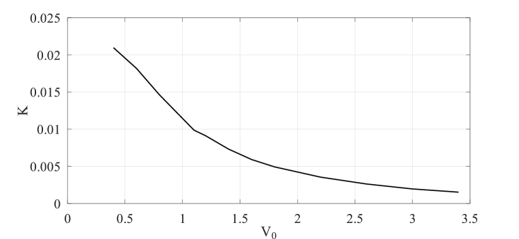
Figure 1: The dependence of the amplitude of the tunneling K on the potential barrier $V_{0}$. Here, $\gamma=0.1$, $l_{\perp}/l_{x}=0.1$,  $l=1$

.

4 Two-mode model with LHY term

Below we will study symmetric case $E_{1}=E_{2}$. Introducing variables:

$$u=\rho_{1}e^{i\theta_{1}},\ v=\rho_{2}e^{i\theta_{2}},\ Z=\frac{N_{1}-N_{2}}{N},$$

$$\theta=\theta_{2}-\theta_{1},\ N_{i}=\rho_{i}^{2},\ N=N_{1}+N_{2},$$

where $Z$ is the atomic populations imbalance, $\theta$ is the relative phase, $N$ is the total number of atoms, indices {$1,2$} relate to the corresponding trap potential wells and substituting these variables into Eqs. (10) and (11), we obtain a set of equations:

$$Z_{t}=-2K\sqrt{1-Z^{2}}\sin(\theta),$$ (12)

$$\theta_{t}=\bar{\gamma}NZ+\frac{2KZ}{\sqrt{1-Z^{2}}}\cos(\theta)+\bar{g}\sqrt{\frac{N}{2}}[(1-Z)^{1/2}-(1+Z)^{1/2}].$$ (13)

The set of equations has the Hamiltonian:

$$H=\frac{\bar{\gamma}N}{2}Z^{2}-2K\sqrt{1-Z^{2}}\cos(\theta)-\bar{g}\frac{\sqrt{2N}}{3}[(1-Z)^{3/2}+(1+Z)^{3/2}].$$ (14)

The hamiltonian equations for the canonical variables $Z,\theta$ are:

$$Z_{t}=-\frac{\partial H}{\partial\theta},\ \theta_{t}=\frac{\partial H}{\partial z}.$$

Stationary states are defined by fixed points of the set ((12), (13)): $Z_{t}=\theta_{t}=0$. The symmetric states are:

$$\theta_{c}=2n\pi.$$

The ground state energy is:

$$E_{0}=-2K-\frac{2g}{3}\sqrt{2N},$$

and the asymmetric states with higher energy are:

$$\theta_{c}=(2n+1)\pi.$$

with

$$E_{ex}=2K-\frac{2g}{3}\sqrt{2N}.$$

Then the critical population imbalance can be find from the equation:

$$\bar{\gamma}NZ_{c}=\frac{2KZ_{c}}{\sqrt{1-Z^{2}}}(-1)^{n}-\bar{g}\sqrt{\frac{N}{2}}[(1-Z_{c})^{1/2}-(1+Z_{c})^{1/2}].$$

4.1 Josephson oscillations

Now we consider Josephson oscillations near $\langle Z\rangle=0$. In the case of small oscillations, the two-mode theory works very well, and the expressions for the Josephson frequency can be obtained from Eqs. (12) and (13).

i) The zero-phase mode($\theta=0$). Supposing the amplitude of oscillations of $Z$ and $\theta$ to be small in Eqs (12) and (13) one can find the frequency of Josephson oscillations near $\langle Z\rangle=0$.

$$\omega_{J}=\sqrt{2K(2K+\bar{\gamma}N-\bar{g}\sqrt{N/2})}.$$ (15)

In dimensional variables:

$$\hbar\omega_{J}=\sqrt{(2\bar{K})^{2}+2\bar{K}\alpha N-2\bar{K}\beta\sqrt{N/2}}.$$ (16)

Here, $\alpha=\delta g\int\phi_{1}^{4}dx\$, $\ \beta=\frac{\pi\hbar}{\sqrt{2m}}\int\phi_{1}^{3}$, $\ \bar{K}=-\left[\frac{\hbar^{2}}{2m}\int\phi_{1,x}\phi_{2,x}dx+\int\phi_{1}V(x)\phi_{2}dx\right]$.

In the case of the LHY fluid when $\bar{\gamma}=0$, the frequency of the Josephson oscillations (JO) becomes less than the Rabi frequency. It can be evidence that the system is in the LHY fluid regime. Note that in the quasi-one-dimensional regime, the JO frequency is higher, than the Rabi oscillations frequency [16, 17]. Measuring the oscillation frequency then allows us to find the contribution of the quantum fluctuations.

ii) $\pi$-phase mode($\theta=\pi$). The frequency of the Josephson oscillation is:

$$\omega_{J}=\sqrt{2K(2K-\bar{\gamma}N+\bar{g}\sqrt{N/2})}.$$ (17)

In dimensional variables:

$$\hbar\omega_{J}=\sqrt{(2\bar{K})^{2}-2\bar{K}\alpha N+2\bar{K}\beta\sqrt{N/2}}.$$ (18)

4.2 Self-trapping regime

Self-trapping regime means that in each well the atoms are localized, i.e. $\langle Z\rangle\neq 0$. ST mode occurs depending on the values of $Z(0)$ and $\gamma$ We can determine the critical values of $Z_{c}$ and $\theta_{c}$ using the Hamiltonian.

The transition condition to the self-trapping regime is determined as follows. Let us rewrite the Hamiltonian by introducing new parameters:

$$\bar{H}=\frac{\Lambda Z^{2}}{2}-\sqrt{1-Z^{2}}cos(\theta)-\delta\left[(1-Z)^{3/2}+(1+Z)^{3/2}\right].$$ (19)

Here, $\bar{H}=H/2K,\ \Lambda=\bar{\gamma}N/(2K),\ \delta=\bar{g}\sqrt{2N}/(6K)$.

Fixing $Z(0),\theta(0)$, we obtain the condition for the self-trapping:

$$\bar{H}>-1-2\delta$$

Then we can obtain a critical value of the parameter $\Lambda$ when the self-trapping occurs:

$$\Lambda_{c}=\frac{2}{Z(0)^{2}}\left[-1+\sqrt{1-Z(0)^{2}}cos(\theta)-\delta(2-(1-Z)^{3/2}-(1+Z)^{3/2})\right].$$ (20)

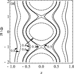
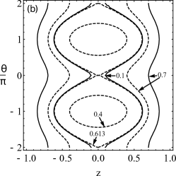
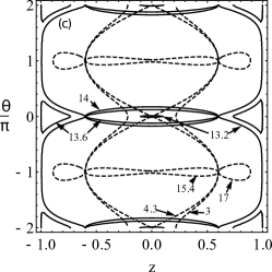
Figure 2: First two phase portraits are shown for the parameters $\Lambda=0$, $\delta=9.6$ (LHY fluid)(a) and $\Lambda=4.81$, $\delta=9.3$(b) in the different initial values of the relative imbalance $Z(0)$. Third phase portrait is presented for different values of $\Lambda$ when $\delta=9.3$ and $Z(0)=0.6$ (c). In all cases, the dashed line is for $\pi$-phase mode and the solid line is for zero-phase mode.

In Fig. 2(a), the phase portraits is plotted using Eq. (19) for the particular case of so-called LHY fluid with $\gamma=0$ at different initial values of the relative imbalance $Z(0)$. The LHY fluid corresponds to the case when the residual mean field is equal to zero $\Lambda=0$, so the nonlinearity in the GP equation is given only by quantum fluctuations [21, 22]. From this graph we can determine the critical value of $Z(0)$, $Z(0)_{c}\approx 0.504$ for $\pi$-phase mode. This critical value satisfies Eq. (20). In the zero-phase mode, there is a localization of the relative imbalance $Z(t)$ for all initial values of $Z(t)$. The relative phase is not localized even in the self-trapping regime in both zero- and $\pi$-phase modes.

In Fig. 2(b), the phase portrait is presented for the parameters $\Lambda=4.81$, $\delta=9,3$ in different initial values of $Z(t)$. This phase portrait is similar to the first one, only here the critical value for Z(0) is slightly larger than the first one, $Z(0)_{c}=0.613$. This critical value satisfies Eq. (20).

In Fig. 2(c), the phase portrait is presented for different values of $\Lambda$ when $\delta=9.3$ and $Z(0)=0.6$. Both phase modes have Josephson oscillations and ST mode. We can determine the critical values using Eq. (20), $\Lambda_{c}\approx 13.2$ for the zero-phase mode and $\Lambda_{c}\approx 4.3$ for the $\pi$-phase mode. Of course, another critical value can be seen from the graph in the $\pi$-phase mode $\Lambda=15.4$, but this point is unstable based on Eq. (17).

The dependence of the frequency of the Josephson oscillations on the residual mean-field interaction strength is presented in Fig. 3.

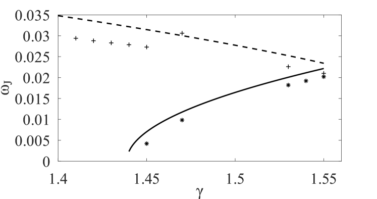
Figure 3: Dependencies of the frequency of the Josephson oscillations on the residual mean-field parameter $\gamma$. The solid and dashed lines stand for the zero-phase, Eq. (15), and $\pi$-phase modes, Eq. (17), respectivelly. The asterisk and symbols $+$ are calculated using numerical simulations for the zero-phase and $\pi$-phase modes, respectively.

The figure shows a good agreement of the two-mode model predictions with full simulations for $\gamma$ around $1.52-1.55$. According to Eq. (15), the Josephson frequency becomes complex at $\gamma\leq 1.43$. This can also be seen from the lower curve in the graph. Therefore, when $\gamma\leq 1.43$, the Josephson oscillation does not exist, where only the ST regime exists. If we change the value of $\gamma$ to $\Lambda$, we can compare this result with the phase portrait results in Fig. 2, for $\gamma=1.43$, $\bar{\gamma}\approx 1.43\times 0.19364$, $\bar{g}\approx 0.42625$, $K\approx 0.0114$, $\Lambda=\bar{\gamma}N/(2K)\approx 9.6$. It can be seen from Fig 2a,b, ST regime exists for all values of $Z(0)$, with $\Lambda\leq 9.6$ for zero-phase mode. The upper curve in Fig. 3 corresponds to the $\pi$-phase mode. In this mode, the Josephson frequency is not complex, so, both, the regime of the Josephson oscillations and the ST regime can exist. This result corresponds to the result in Fig. 2.

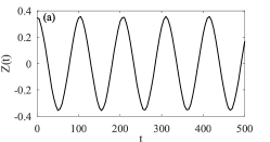
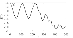
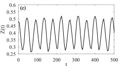
Figure 4: The dynamics of the relative imbalance ($Z(t)$) is presented for LHY fluid case ($\gamma=0$). Here, $Z(0)=0.36$ (a), $Z(0)=0.38$ (b), $Z(0)=0.5$(c). For all cases $V_{0}=1$, $\Omega=0.1$, $l=0.5$.

The graphs Figs 4a,b,c depict the transition of the dynamics of imbalance Z(t) from the Josephson oscillation regime to the ST regime for the LHY fluid ($\gamma=0$). We can determine the critical value of $Z(0)$, $Z(0)=Z_{c}=0.38$ in these graphs. From the figures, it can be seen that Josephson oscillations appear, when the condition $Z(0)<Z_{c}$ is met. When the condition $Z(0)>Z_{c}$, the dynamics of $Z(t)$ goes into the ST regime.

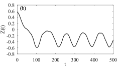
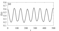
Figure 5: The dynamics of the relative imbalance ($Z(t)$) are presented for $\gamma=0.5$ $(\Lambda\approx 4.81)$. Here, $Z(0)=0.5$ (a), $Z(0)=0.57$ (b), $Z(0)=0.6$(c). For all cases $V_{0}=1$, $\Omega=0.1$, $l=0.5$.

The graphs Figs 5a,b,c depict the transition of the dynamics of imbalance Z(t) from the Josephson oscillation regime to the ST one for $\gamma=0.5$). We can determine the critical value of $Z(0)$, viz. $Z(0)=Z_{c}=0.57$ in these graphs. The Josephson oscillations appear, when the condition $Z(0)<Z_{c}$ is met, and the dynamics of $Z(t)$ goes into the ST regime. The two-mode model predicts that the threshold value of the $\bar{\gamma}$ is increased in the one-dimensional geometry when the LHY correction is taken into account, at the same time in the quasi-one-dimensional case, it is reduced, in comparison with the mean-field value [17, 16]. The full numerical simulations confirm this prediction. But theoretical and numerical values agreed only quantitatively, due to well-known limitations of the two-mode model [23].

5 Modulated in time tunneling

Let us study the Josephson oscillations when the barrier is periodically modulated in time:

$$V(x)=\frac{\Omega^{2}}{2}x^{2}+(V_{0}+V_{1}sin(\omega t))sech^{2}\left(\frac{x}{l}\right).$$ (21)

Such modulation leads to the oscillating in time of the macroscopic tunneling coefficient $K$:

$$K(t)=K_{0}+K_{1}\sin(\omega t),$$ (22)

where

$$K_{0}=-\left[\frac{1}{2}\int dx\phi_{1,x}\phi_{2,x}+\int dx\phi_{1}V_{0}\phi_{2}\right],\ K_{1}=-\left[\int dx\phi_{1}V_{1}sech^{2}(x/l)\phi_{2}\right]$$

. This procedure represents one of the ways to control the macroscopic quantum tunneling of BEC in the double-well trap [24, 25, 26, 27].

Considering small oscillations of $Z,\theta$ near zero values, we obtain the equation for the populations imbalance:

$$\delta Z_{tt}+\omega_{0}^{2}(1+h\sin(\omega t))\delta Z-\frac{K_{1}\omega}{K_{0}}\cos(\omega t)\delta Z_{t}=0,$$ (23)

where

$$\omega_{0}^{2}=2K_{0}\left(2K_{0}+\gamma N+\sqrt{\frac{N}{2}}\right),\ h=\frac{K_{1}}{K_{0}}\left(1+\frac{4K_{0}^{2}}{\omega_{0}^{2}}\right).$$

The standard analysis [28], shows that the parametric resonance in the oscillations of the imbalance exists at

$$\omega=2\omega_{0}.$$

The gain at the parametric resonance $\lambda$ is:

$$\lambda=\sqrt{\beta-\frac{\delta^{2}}{4}},\ \ \beta=\left(\frac{K_{1}}{8K_{0}}-h\right)\frac{\omega_{0}^{2}}{4}.$$ (24)

Note, that when the nonlinearities are equal to zero, in the case of Rabi oscillations, the gain is equal to zero and parametric resonance (PR) is absent. It can be seen also from the initial dimer equations Eq. (11) in the linear limit, since in this case the modulations of $K(t)$ can be removed from the equations by redifinition of the time as $\tau=\int K(t)dt$. One of the important consequences is that using the PR for the LHY fluid (with $\gamma=0$ [21]) we can measure the strength of quantum fluctuations.

In Figs  6 and 7 the results of numerical simulations obtained from the two-mode theory and full GP equation with double-well potential are presented. The gain at the resonance is agreed well, while the long time dynamics is described qualitatively. it is connected with the approximate character of the two-mode model, neglecting the nonlinear corrections to the tunneling coefficients $K$.

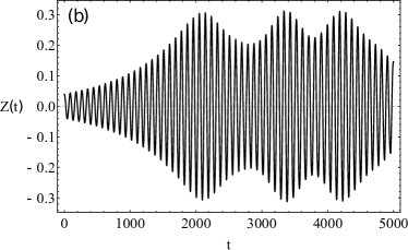
Figure 6: The parametric resonances for $\Omega=0.1$,$V_{0}=1$, $l=0.5$, $V_{1}=V_{0}/20$, $\omega=2\omega_{J}$, are shown at $\gamma=0$. These results are obtained using the two-mode theory (a) and the numerical simulations method (b).

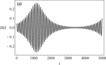
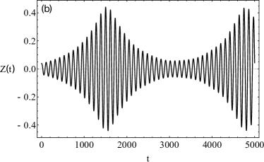
Figure 7: The figure depicts parametric resonances for $\Omega=0.1$,$V_{0}=1$, $l=0.5$, $V_{1}=V_{0}/10$, $\omega=2\omega_{J}$, at $\gamma=0.5$. Results are obtained using the two-mode theory (a), and the numerical simulations method (b).

6 Conclusion

We have investigated the nonlinear dynamics of BEC loaded in a double-well potential. The beyond mean-field corrections to the energy in the form of the Lee-Huang-Yang term are taken into account. We derive a two-mode model to describe analytically the dynamics of BEC. Using this model we obtain the expressions for the frequencies of the Josephson oscillations when the contribution of the quantum fluctuations are taken into account. The threshold value of the residual mean field nonlinearity, when switching from the MQT regime to the ST regime occurs, has been found. The results applied for the description of the dynamics of the quasi-one-dimensional LHY superfluid in the double-well potential. The parametric resonance in the Josephson oscillations when the barrier is periodically modulated, is studied. The analytical predictions are compared with the full numerical simulations of the modified GP equation, showing good agreement.

7 Acknowledgments

We thank B. B. Baizakov and E. N. Tsoy for fruitful discussions. This work has been implemented within the research topic of the Laboratory of Theoretical Physics of Physical-Technical Institute of Uzbekistan Academy of Sciences, funded by the State Budget of Uzbekistan (Grant No. 2024 year award). F.Kh.A. acknowledges the support of the Ministry of Higher Education, Science and Innovation of the Republic of Uzbekistan (Grant No. ALM-2023-1006-2528).

8 Author contributions

All the authors contributed equally to this work. All the authors have read and approved the final manuscript.

References

- [1] T.D. Lee, K. Huang, and C.N. Yang, Phys. Rev. 106 1135 (1957).
- [2] D.S. Petrov, Phys.Rev.Lett. 115 155302 (2015). https://doi.org/10.1103/PhysRevLett.115.155302
- [3] D.S. Petrov and G.E. Astrakharchik, Phys.Rev. Lett. 117 100401 (2016). https://doi.org/10.1103/PhysRevLett.117.100401
- [4] C.R. Cabrera, L. Tanzi, J. Sanz, B. Naylor, P. Thomas, P. Cheiney, and L. Tarruell, Science 359 301 (2018).
- [5] G. Semeghini, G. Ferioli, L. Masi, C. Mazzinghi, L. Wolswijk, F. Minardi, M. Modugno, G. Modugno, M. Inguscio, and M. Fattori, Phys. Rev. Lett. 120, 235301 2018.
- [6] I. Ferrier-Barbut, H. Kadau, M. Schmitt, M. Wenzel, T. Pfau, Phys. Rev. Lett. 116 215301 (2016).
- [7] L. Chomaz, S. Baier, D. Petter, M.J. Mark, F. Wächtler, L. Santos, and F. Ferlaino, Phys. Rev. X 6, 041039 (2016).
- [8] M. Schmitt, M. Wenzel, F. Böttcher, I. Ferrier-Barbut, and T. Pfau, Nature (London)539, 259 (2016).
- [9] F. Böttcher, J.-N. Schmidt, J. Hertkorn, K.S.H. Ng, S.D. Graham, M. Guo, T. Langen, and T. Pfau, Rep. Prog. Phys. 84 012403 (2021).
- [10] Z. Luo, W. Pang, B. Liu, Y. Li, and B.A. Malomed, Frontiers in Physics, 16, 32201 (2021).
- [11] M.R. Pathak, A. Nath, Scientific Reports 12 6904 (2022).
- [12] Y.V. Kartashov, M. Lashkin, M. Modugno, and L. Torner, New J. Phys. 24 073012 (2022).
- [13] Sh.R. Otajonov, E.N. Tsoy, and F.Kh. Abdullaev, Phys. Rev. A 106 033309 (2022)
- [14] D. Edler et al., Phys.Rev.Research, 4, 033017 (2022).
- [15] S. Raghavan, A. Smerzi, S. Fantoni, and S.R. Shenoy, Phys. Rev. A 59 620 (1999). https://doi.org/10.1103/PhysRevA.59.620
- [16] F.Kh. Abdullaev, R.M. Galimzyanov, and A. Shermakhmatov, J.Phys. B 56 165301 (2023). https://doi.org/10.1088/1361-6455/ace66d
- [17] A. Bardin, F. Lorenzi, L. Salasnich, New J. Phys. 26, 013021 (2024). https://doi.org/10.1088/1367-2630/ad127b
- [18] T. Mithun et al., Symmetry, 12(1), 174 (2020).
- [19] X. Hu, Z. Li, Y. Guo, Y. Chen, and X. Luo, Phys. Rev. A 108, 053306 (2023).
- [20] A. Debnath, A. Khan, B. Malomed, Comm. in Nonl. Sci. and Num. Sim. 126, 107457 (2023).
- [21] N.B. Jorgensen et al., Phys.Rev. Lett. 121 173403 (2018). https://doi.org/10.1103/PhysRevLett.121.173403
- [22] T.G. Skov et. al., Phys.Rev.Lett. 126 230404 (2021).
- [23] D. Ananikian, and T. Bergeman, Phys. Rev. A 73 013604 (2006). https://doi.org/10.1103/PhysRevA.73.013604
- [24] F.Kh. Abdullaev, and R.A. Kraenkel, Phys. Rev. A 62 023613 (2000). https://doi.org/10.1103/PhysRevA.62.023613
- [25] F.Kh. Abdullaev, and R.A. Kraenkel, Phys. Lett. A 272 395 (2000). https://www.sciencedirect.com/science/article/pii/S0375960100004357
- [26] G.L. Salmond, C.A. Holmes, and G.J. Milburn, Phys.Rev. A 65 033623 (2002).
- [27] E. Boukobza, M.G. Moore, D. Cohen, and A. Vardi, Phys.Rev.Lett. 104 240402 (2010).
- [28] Landau L, Lifshitz E 1975 Mechanics, Pergamon.