OpenMaterial: A Comprehensive Dataset of Complex Materials for 3D Reconstruction

Abstract

Recent advances in deep learning such as neural radiance fields and implicit neural representations have significantly propelled the field of 3D reconstruction. However, accurately reconstructing objects with complex optical properties, such as metals and glass, remains a formidable challenge due to their unique specular and light-transmission characteristics. To facilitate the development of solutions to these challenges, we introduce the OpenMaterial dataset, comprising 1001 objects made of 295 distinct materials—including conductors, dielectrics, plastics, and their roughened variants— and captured under 723 diverse lighting conditions. To this end, we utilized physics-based rendering with laboratory-measured Indices of Refraction (IOR) and generated high-fidelity multiview images that closely replicate real-world objects. OpenMaterial provides comprehensive annotations, including 3D shape, material type, camera pose, depth, and object mask. It stands as the first large-scale dataset enabling quantitative evaluations of existing algorithms on objects with diverse and challenging materials, thereby paving the way for the development of 3D reconstruction algorithms capable of handling complex material properties.

1 Introduction

Recovering the physical 3D layout of a scene from a series images has been a long-standing and fundamental problem in computer vision. Successfully achieving such 3D reconstruction would facilitate many downstream tasks such as augmented/virtual/mixed reality, environment mapping for autonomous navigation, or creating digital twins of the real world using ubiquitous mobile devices.

In recent years, the field of 3D reconstruction has seen significant progress, particularly via the development of neural radiance fields, which, although often targeting novel view synthesis, aim to internally extract a 3D scene representation. In this context, while the pioneering NeRF method simply modeled 3D shape as an occupancy map, subsequent approaches have introduced the use of implicit neural representations, such as deep signed distance functions, thus leveraging popular 3D shape models. Among these, variants such as Neuralangelo [1], BakedSDF [2], and Instant-NGP [3] achieve peak performance in their respective areas. However, a closer inspection of the performance of these algorithms reveals that they may produce unsatisfactory results depending on the material properties of the observed object. For example, as noted in [4], Neuralangelo yields geometric distortions when processing a metal rabbit model; similarly, BakedSDF produces artifacts when reconstructing a toaster with a specular surface. Altogether, it thus appears that, while existing 3D reconstruction algorithms deliver nearly perfect results on objects with diffuse surfaces, they consistently fail in the presence of objects that exhibit complex optical properties, such as those made of metal, glass, etc. This is because the complexity of light refraction, transmission, and specular reflection on such objects leads to color inconsistencies across the multiple views, thus violating the underlying assumption of existing methods and posing significant challenges for 3D reconstruction.

One of the key obstacles in the development of 3D reconstruction methods for non-diffuse objects is the lack of a standardized dataset covering a large diversity of complex materials and object shapes. To this date, only the dataset of [5] introduces some challenging materials but remains limited to 8 objects. This, however, falls short of providing a comprehensive benchmark for evaluating an algorithm’s abilities at successfully handling diverse material types.

In this paper, we introduce a comprehensive dataset, dubbed OpenMaterial, featuring a wide array of challenging materials, diverse shapes, and lighting conditions. To address the challenge of obtaining a large-scale, diverse collection with ground-truth 3D shapes, we exploit physics-based rendering to generate dense multiview images with exceptional realism. OpenMaterial encompasses 295 distinct material types covering seven categories, encompassing conductors, dielectrics, and plastics. This includes 294 materials with laboratory-measured Index of Refraction (IOR) values representing real-world materials, and one idealized diffuse material. Our dataset also includes 1001 unique geometric shapes to ensure shape diversity and features 723 diverse environmental lighting conditions, replicating a broad spectrum of indoor and outdoor scenarios.

OpenMaterial’s extensive diversity in material types, geometric shapes, and lighting conditions not only supports comprehensive evaluations but also enables a detailed analysis of the capabilities of existing algorithms in handling challenging materials. We demonstrate this by evaluating state-of-the-art (SOTA) 3D reconstruction and novel view synthesis algorithms using our dataset. To the best of our knowledge, OpenMaterial is the first dataset specifically designed for the quantitative assessment of 3D reconstruction methods targeting objects with complex materials. To facilitate future work, the data and evaluation protocol can be accessed at https://christy61.github.io/openmaterial.github.io/.

2 Related Work

Multi-view 3D Reconstruction. Traditional multi-view 3D reconstruction methods, as referenced in numerous studies [6, 7, 8, 9, 10, 11, 12, 13, 14, 15, 16], employ geometric principles and often depend on color consistency to detect and match points across multiple images. These methods are primarily effective for static scenes with diffuse reflection. Learning-based approaches [17, 18, 19, 20, 21, 22, 23, 24, 25] seek to predict 3D structure from images. However, to generalize across scenes, these methods require large amounts of annotated data for training. NeRF (Neural Radiance Fields) [26], initially designed for novel view synthesis [3, 27, 28, 29, 30], have been rapidly extended to 3D reconstruction beyond discrete points by incorporating implicit surface representations [31, 32, 33, 34, 2, 35, 1] to produce smooth, continuous surfaces. For a review of NeRF-based 3D reconstruction please see [36]. Despite this progress, handling complex material properties in 3D reconstruction remains challenging; only a few attempts such as [5, 37] aim to integrate BSDF into the neural field optimization process, thus enhancing the capability to deal with complex materials. Importantly, there is currently no extensive benchmark to evaluate such efforts at pushing the boundaries of the NeRF-based approach.

Existing Dataset.

Most real [38, 27, 39, 40, 41, 42] and synthetic [26, 38, 27] datasets designed for relighting and novel view synthesis typically do not capture 3D shape, which is critical to evaluate 3D reconstruction. While a few real datasets [43, 44, 45, 46, 47, 48, 49] feature objects composed of mixed materials with 3D annotations, the amount of objects and proportion of complex materials are relatively small. An exception is the NeRO [5], which contains eight objects with smooth, shiny metal surfaces, providing better material complexity. Given the challenges in capturing real objects, efforts have shifted towards synthetic data creation. ShapeNet-Intrinsics [50] contains a large number of 3D shapes rendered in multiple view images using a basic Phong model. BlendedMVS [51] uses textured 3D models to render multiple viewpoints, assuming the textured surfaces are diffuse. Meanwhile, Objaverse [52] contains extensive 3D models collected from open-source 3D design websites, and ABO [53] collects a substantial number of artist-created 3D models of household objects; however, the materials are defined by color, roughness, metallic, and transparency, which may not faithfully replicate the nuanced behaviors observed in real-world materials. Specific datasets like [43, 5] target material properties but are restricted to under twenty objects focusing on simple diffuse and reflective surfaces, omitting complex material behaviors such as refraction and transmission. In this work, we leverage the Objaverse 3D shapes, but exploit laboratory-measured IOR within a physics-based rendering framework to create the first comprehensive realistic dataset featuring complex materials, thus aiming to facilitate future research in 3D reconstruction in challenging conditions.

3 Dataset Construction

Our objective is to create a dataset that enables a comprehensive evaluation of existing 3D reconstruction algorithms across a variety of materials, shapes, and lighting conditions. Our dataset encompasses seven material types: Diffuse, conductor, dielectric, plastic, rough conductor, rough dielectric, and rough plastic, totaling 295 distinct types. It comprises 1001 scenes, where each scene features a unique shape and a single randomly selected material. The lighting conditions are also chosen randomly from 723 available High Dynamic Range Imaging(HDRI) environmental lighting options. To create a balanced dataset, each of the seven material categories is represented in 143 scenes. Besides multi-view images from multiple camera positions, the dataset includes 3D mesh models, material annotations, camera poses, depth maps, and object masks, providing a rich set of data for in-depth analysis and testing.

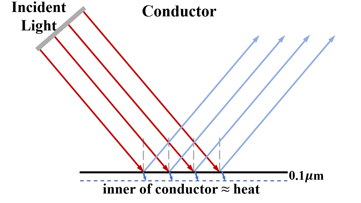
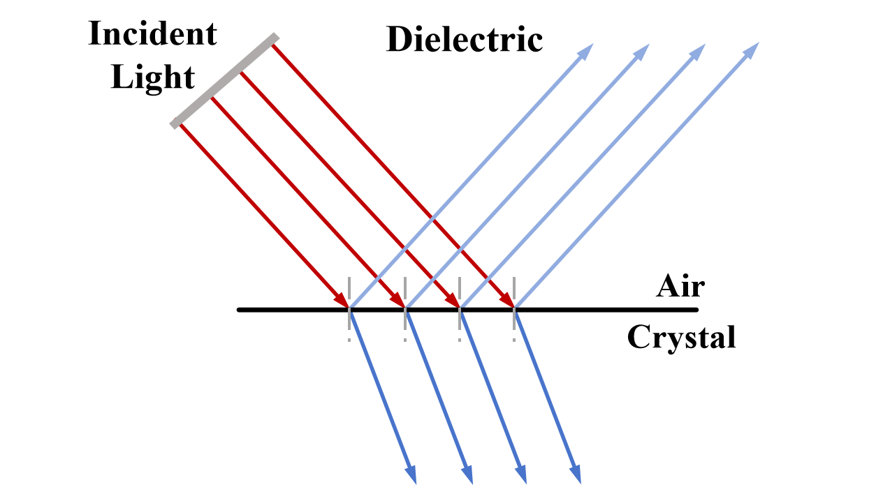
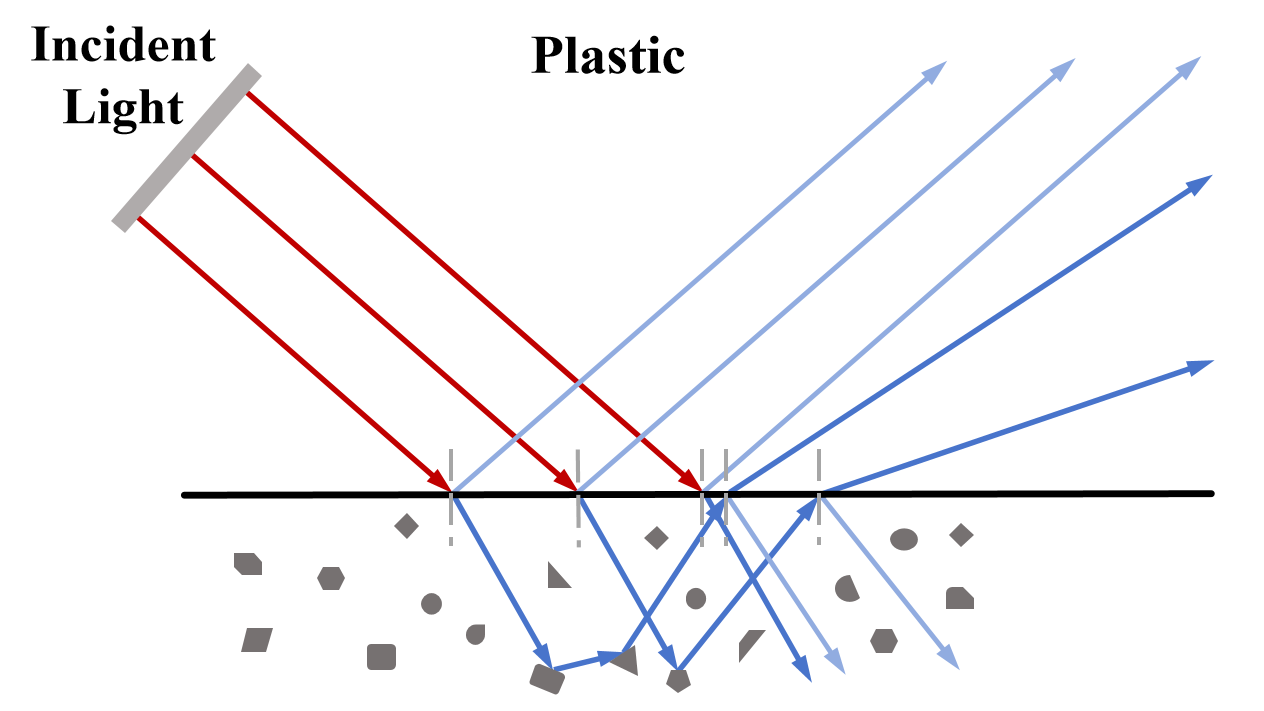
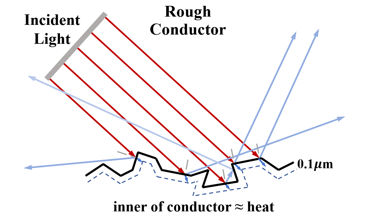
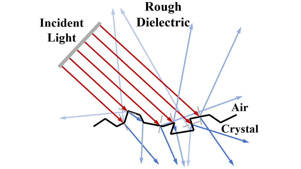
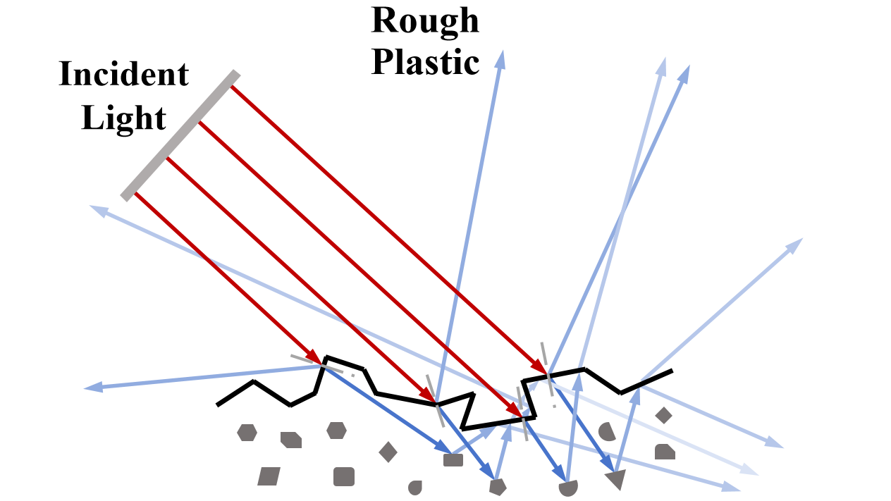
Figure 1: Illustration of light interaction with various materials.

3.1 Physically-based Rendering

In the real world, each material interacts with light in different ways, presenting specific appearance and challenges in the image. The Bidirectional Scattering Distribution Function(BSDF) plays a crucial role in the rendering process by defining how light interacts with surfaces at a detailed and physically-accurate level. It encapsulates both how light is reflected off surfaces, as described by the Bidirectional Reflectance Distribution Function (BRDF), and how light transmits through materials, as characterized by the Bidirectional Transmission Distribution Function (BTDF). This dual capability allows for accurate simulation of complex optical properties such as specular reflection, glossiness, and transmission. Once the BSDF is established for a material, the rendering engine can compute the color and intensity of light reflecting and transmitting at different points on the surface. The RGB values for each pixel in the final image are derived by integrating the light from all incoming directions, factoring in the material properties defined by the BSDF, to realistically capture the appearance of materials under varied lighting conditions.

Figure 2: Distinct materials. From left to right: conductor, dielectric, plastic and diffuse. The top portion of the vase shows rough surface finishes, while the bottom one shows smooth surface finishes.

Formally, given the normal direction $\omega_{n}$ of a point on the object surface, the direction of the incident light $\omega_{i}$, and the directions of outgoing light (reflected as $\omega_{r}$ and refracted as $\omega_{t}$), the BSDF $f_{s}$ of the surface material of the object can be expressed as the sum of the BRDF $f_{r}$ and the BTDF $f_{t}$, i.e.,

$$f_{s}=f_{r}+f_{t}\;.$$

The BRDF and BTDF [54] for microsurface reflection and refraction are defined as

$$f_{r}=\frac{\mathcal{F}(\omega_{i},\omega_{h})\mathcal{G}(\omega_{i},\omega_{r},\omega_{h})\mathcal{D}(\omega_{h})}{4|\omega_{i}\cdot\omega_{n}||\omega_{r}\cdot\omega_{n}|},$$

$$f_{t}=\frac{|\omega_{i}\cdot\omega_{h}||\omega_{t}\cdot\omega_{h}|}{|\omega_{i}\cdot\omega_{n}||\omega_{t}\cdot\omega_{n}|}\frac{\eta_{t}^{2}(1-\mathcal{F}(\omega_{i},\omega_{h}))\mathcal{G}(\omega_{i},\omega_{t},\omega_{h})\mathcal{D}(\omega_{h})}{(\eta_{i}(\omega_{i}\cdot\omega_{h})+\eta_{t}(\omega_{t}\cdot\omega_{h}))^{2}}$$

where $\omega_{h}$ represents the intermediate vector between the $\omega_{i}$ and $\omega_{r}$. For BRDF $\omega_{h}=sign(\omega_{i}\cdot\omega_{n})(\omega_{i}+\omega_{r})$, for the BTDF, the $\omega_{h}$ definition is different, where $\omega_{h}=-(\eta_{i}\omega_{i}+\eta_{t}\omega_{t})$. For ideal reflection and idea refraction, the $\omega_{h}$ as same as the normal direction $\omega_{n}$, further details can be found in [54]. $\mathcal{F}$ is determined using Fresnel’s equation [55] (see below), $\mathcal{G}$ is the shadow occlusion function, which we define here as Smith’s shadow-masking function [54], and $\mathcal{D}$ is the microfacet normal distribution function. Finally, $\eta_{i}$ and $\eta_{t}$ represent the IOR of the initial and transmitted media, one of which is air in our setting.

To capture the characteristics of real-world materials, our simulations employ laboratory-measured Indices of Refraction (IOR). Both the angle(Snell’s law) and the intensity(Fresnel’s equation) of outgoing light are accurately calculated based on the IOR. By integrating these well-established physical laws with real-world measured IORs, we establish a solid foundation for our dataset, ensuring highly accurate and realistic simulations.

Snell’s law. Let $\theta_{i}$, $\theta_{r}$, $\theta_{t}$ represent the angles between $\omega_{i}$ and $\omega_{n}$, between $\omega_{r}$ and $\omega_{n}$, and between $\omega_{t}$ and $\omega_{n}$, respectively. For specular reflection, we directly have $\theta_{i}=\theta_{r}$. By contrast, for transmitted light in transparent materials, the angle $\theta_{t}$ can be calculated using the IOR via Snell’s Law [55] as

$$\theta_{t}=arcsin(\frac{\eta_{i}\sin\theta_{i}}{\eta_{t}})\;.$$

Fresnel’s equation. Once the angle of the outgoing light is determined, Fresnel’s equation can be used to determine the precise amount of light reflected and transmitted at the interface between two media. For the reflected amount of light $\mathcal{F}$, Fresnel’s equation is expressed as

$$\mathcal{F}=\frac{1}{2}(r_{\parallel}^{2}+r_{\perp}^{2}),\quad r_{\parallel}=\frac{\eta_{t}\cos\theta_{i}-\eta_{i}\cos\theta_{t}}{\eta_{t}\cos\theta_{i}+\eta_{i}\cos\theta_{t}},\quad r_{\perp}=\frac{\eta_{i}\cos\theta_{i}-\eta_{t}\cos\theta_{t}}{\eta_{i}\cos\theta_{i}+\eta_{t}\cos\theta_{t}}\;.$$

The quantity of transmitted light, such as the light passing through the dielectric material, can be calculated as $1-\mathcal{F}$, reflecting the energy conservation principles. For conductors, a complex IOR includes an imaginary part that accounts for light absorption, as detailed further in the appendix.

3.2 Material Types

Let us now describe the material types and the microfacet model we used to create our dataset.

Conductors are characterized by their free electrons that can move easily throughout the material. Upon illumination, these free electrons absorb and re-radiate the electromagnetic waves, resulting in most of the incident light being reflected, as shown in Fig. 1. This high reflectivity is why metals typically exhibit a shiny, reflective surface, as shown in Fig. 2. Any light that penetrates the surface is absorbed within the first 0.1 $\mu m$, converting quickly to heat and rendering the metal opaque. Due to the rapid absorption and conversion of transmitted light into heat, we specifically choose to model only the reflection component using the BRDF in the rendering processes, simplifying the simulation of conductor surfaces.

Dielectric such as glass and pure water lack free electrons, which are essential for electrical conductivity; thus, unlike conductors, light is able to pass through these materials without being absorbed, as shown in Fig. 1. This attribute grants them their notable transmissive properties and transparent appearance, as depicted in Fig. 2. The interaction of light with a dielectric material, influenced by its transparency and internal structure, can result in either transmission or reflection. We model these behaviors in simulation using the BRDF for reflection and the BTDF for transmission.

Plastics polymers derived from organic compounds belong to a subgroup of dielectrics and exhibit similar properties such as reflection and refraction. Their unique molecular structure, coupled with the inclusion of internal pigments, promotes diffuse reflection Fig. 1, resulting in surfaces that display a blend of glossy specular reflections and softened appearances Fig. 2. These pigments selectively absorb and transmit various light wavelengths, creating a vibrant spectrum of colors. In simulation, plastics are modeled with a reflective and refractive outer layer coupled with a diffused inner layer to provide a nuanced and physically accurate depiction of their light interactions. We employ the BRDF and the BTDF to simulate reflection and transmission, respectively.

Diffuse materials are typically idealized in simulation to highlight their property of scattering the received illumination uniformly, making the surface appear consistent from any viewing direction. To accurately model these materials, we assign a fixed reflectance parameter to the BRDF. To enhance visibility against varying backgrounds, each color is assigned a random gray-scale value ranging from 0.15 to 0.85, ensuring that the materials stand out distinctly from the background.

Microfacet model. Given the BSDF, we exploit a microfacet model to realistically model the microscopic surface details that affect light scattering. Specifically, we adapt the model for smooth and rough surfaces by selecting appropriate microfacets distributions. For materials such as conductors, dielectrics, and plastics with smooth surfaces, we employ the Dirac delta distribution $D(\omega_{h})=\delta(\omega_{h}-\omega_{n})$, which is non-zero only at the surface normal $\omega_{n}$ orientation. This choice ensures sharp and precise reflections and refractions, as evidenced in Fig. 2, effectively simulating the realistic appearance of polished metals, glass, and plastic.

For materials with rough surfaces, including rough conductors, dielectrics, and plastics, we select the Trowbridge-Reitz (GGX) distribution to simulate glossy specular reflections and diffuse refractions. This distribution, characterized by its heavy tail influenced by the roughness parameter $\alpha$, more accurately models the complex scattering of light on these rough surfaces, enhancing physical plausibility and realism in the rendered materials, as illustrated in in Fig. 2. In this case, we have

$$D(\omega_{h})=\frac{\alpha^{2}}{\pi\left(\cos^{2}\theta_{h}(\alpha^{2}-1)+1\right)^{2}}\;,$$

where $\alpha$ is the surface roughness parameter, and $\theta_{h}$ is the angle between $\omega_{h}$ and $\omega_{n}$.

3.3 Laboratory-measured IOR

To ensure that our images mimic real-world materials with physical accuracy, we derive the IOR values from laboratory measurements documented in the optical science literature [56, 57, 58, 59, 60, 61, 62, 61, 63, 64, 65, 66, 67, 68, 69, 70, 71, 72, 67]. Our simulations are thus adjusted to the material at hand to account for variability in IOR across different wavelengths.

For conductors, the IOR varies under different wavelengths of light. For instance, gold absorbs more light at shorter wavelengths (closer to blue light) and reflects more light at longer wavelengths (in the red spectrum), ultimately appearing golden yellow in images. Therefore, we sample spectral data in 5 $nm$ increments within the visible spectrum (380 $nm$ to 780 $nm$). This allows us to accurately simulate the characteristic appearance by capturing its unique light absorption at different wavelengths. Conversely, for dielectrics and plastics, where IOR varies minimally with wavelength changes, we streamline our process by adopting a representative refractive index at 589.29 $nm$. This simplification boosts the rendering efficiency without sacrificing accuracy of the final outputs, ensuring that materials are portrayed with high fidelity yet efficiently.

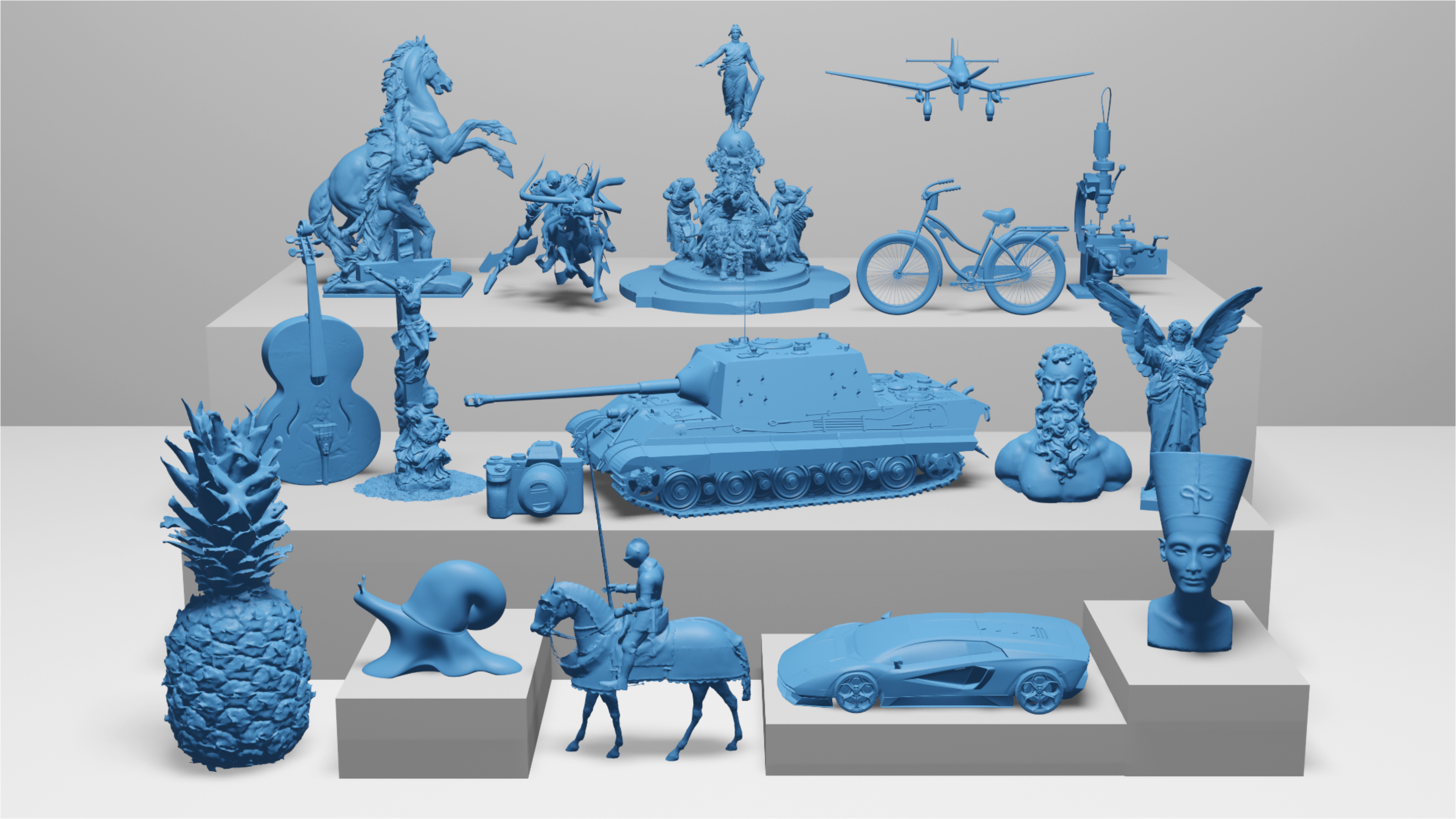
Figure 3: Selection of objects.

3.4 Shapes and Meshes

Our dataset comprises 1,001 unique shapes meticulously selected from the Objaverse-1 dataset [52]. To ensure the diversity and complexity of the shapes, we picked shapes ranging from simple objects, such as guitars, to complex ones, such as fountain statues composed of diverse human poses and intricate facial expressions. A few examples are shown in Fig. 3. The shapes are then randomly distributed across the seven material categories.

3.5 Scene Illumination and Cameras

Figure 4: Illustration of selected HDRI environment maps.

To obtain a high diversity of lighting conditions, we utilized 723 HDRI (High Dynamic Range Imaging) environment maps, encompassing both indoor and outdoor scenarios. These HDRI maps meticulously capture the full spectrum of light intensities found in real-world environments. This not only adds realism to the rendered images but also enables the depiction of complex and varied reflection and refraction patterns on objects, as evidenced in  Fig. 4. The wide range of lighting scenarios provided by these HDRI maps is instrumental in facilitating a thorough evaluation of an algorithm’s effectiveness in handling diverse and challenging lighting conditions.

To eliminate scale bias, we standardize object sizes within a unit sphere. This lets us sample camera positions using a Fibonacci grid on the upper hemisphere, ensuring uniform distribution and non-overlapping coverage. We then splits these camera positions into distinct training (50) and testing (40) viewpoints. All high-resolution images (1600x1200 pixels), rendered using Mitsuba [73], along with associated data including camera positions, depth, 3D object models, and object masks, are stored in the standard Blender format, with support for conversion to the COLMAP format, facilitating usability across the research community.

4 Baseline Experiments

Let us now exploit our dataset to evaluate SOTA methods for two tasks: 3D shape reconstruction and novel view synthesis. Given that our dataset contains a significantly larger number of objects than existing datasets, we opt for faster algorithms capable of converging within 15 minutes per scene. The selected algorithms—Instant-NGP [3], Gaussian-Splatting [74], Instant-NeuS [75], and NeuS2 [35]—have demonstrated state-of-the-art performance in reconstructing 3D shapes and synthesizing novel views from multi-view images.

Conductor	Dielectric	Plastic	Diffuse

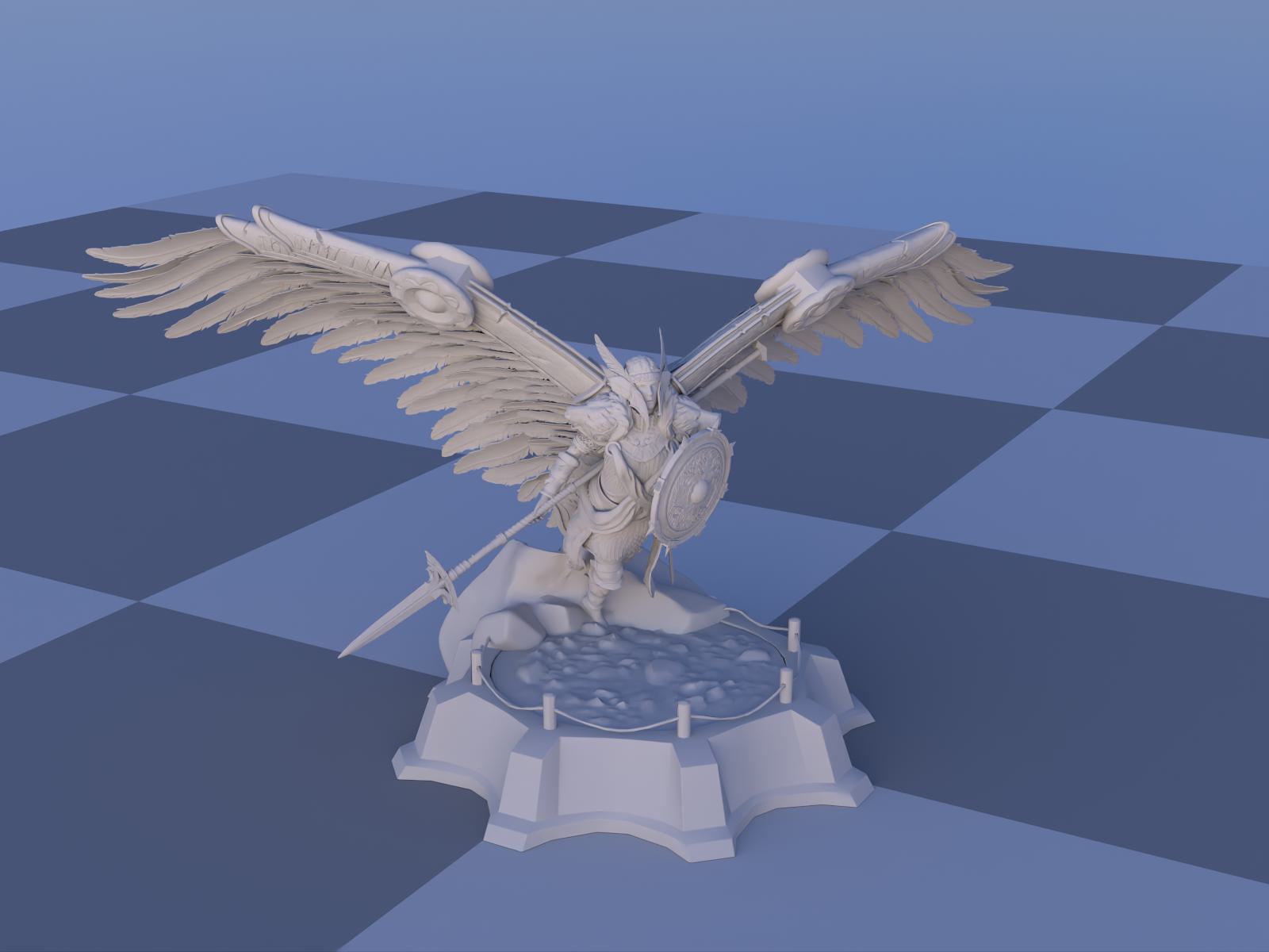
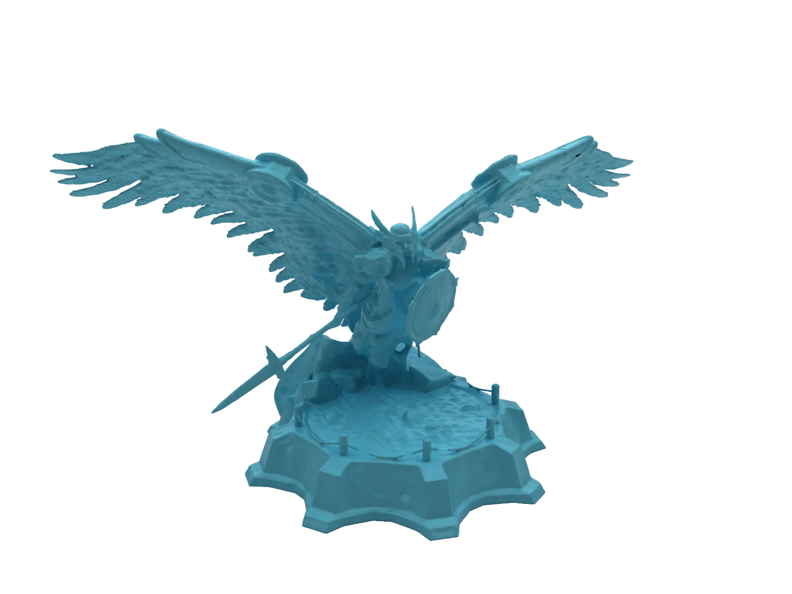
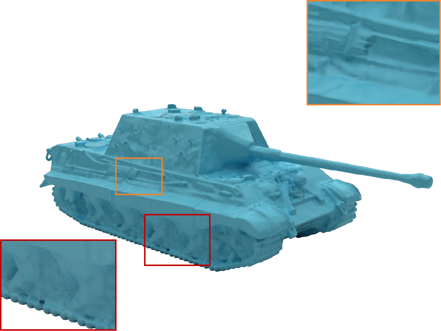
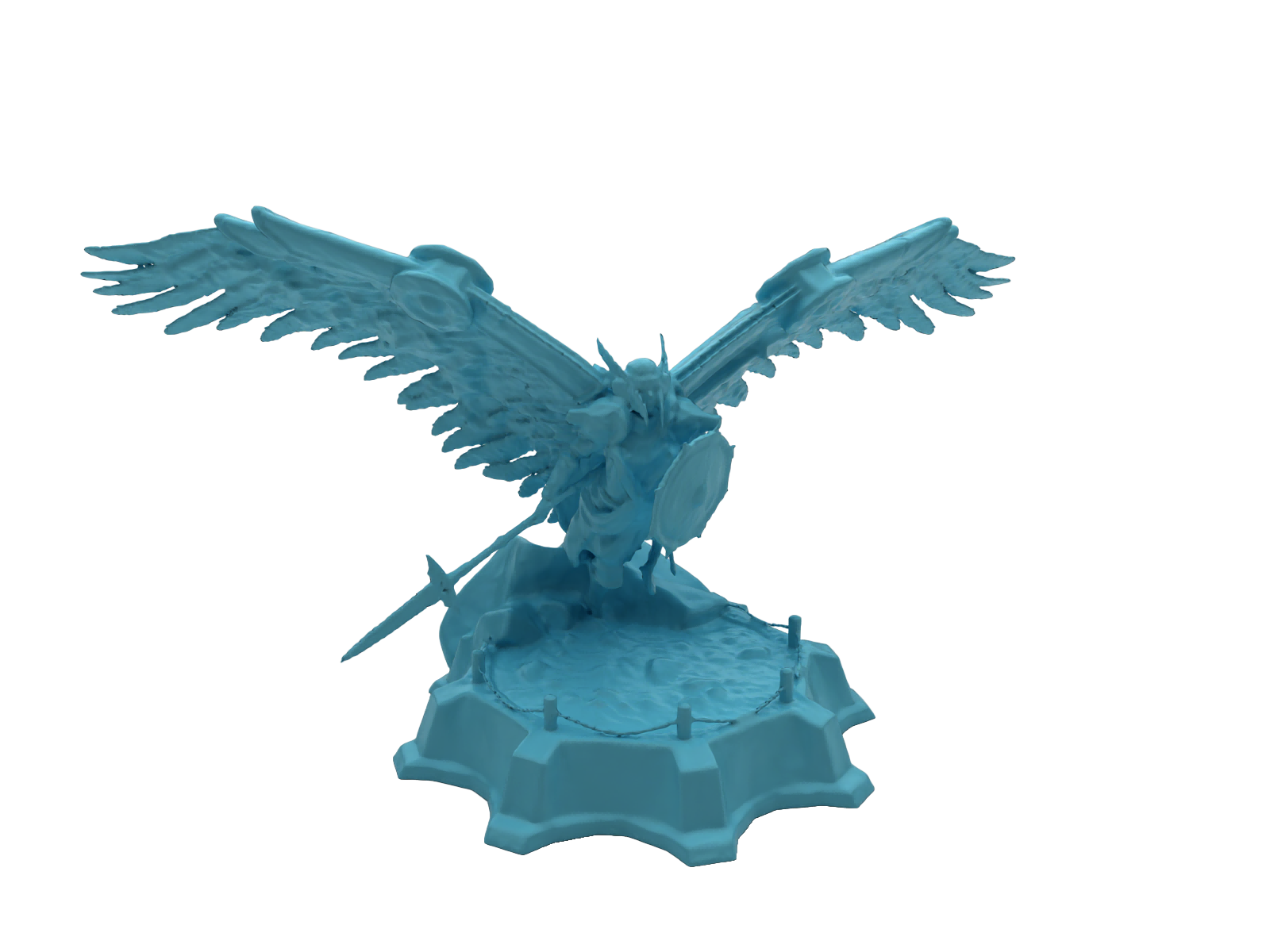
Figure 5: Qualitative 3D reconstruction results. Top row: Input images; Second row: Ground truth; Third row: Instant-NeuS; Bottom row: NeuS2.

4.1 3D Shape Reconstruction

Evaluation metric. In this study, we evaluate 3D shape reconstruction on the visible surface portions. We calculate the Chamfer distance between these point clouds to assess the reconstruction’s accuracy. Consistently with the NeuS [32] evaluation guidelines, we exclude any outlier with a Chamfer distance exceeding 0.15 to improve the result’s reliability. Details regarding the visible ground-truth mesh portion are provided in the appendix.

Table 1: Comparison of Instant-NeuS and NeuS2. We report the Chamfer distance $\times 10^{-2}$.

Method	Material Type
	Conductor	Dielectric	Plastic	Rough Conductor	Rough Dielectric	Rough Plastic	Diffuse
Instant-NeuS[75]	1.2554	1.1912	0.7023	0.9824	1.1634	0.6417	0.6425
NeuS2[35]	1.3016	1.2734	0.6823	1.0192	1.2553	0.6372	0.5998

Results and analysis. We evaluate the performance of two state-of-the-art 3D reconstruction algorithms, Instant-NeuS [75] and NeuS2 [35], across a range of materials with varying optical properties. The Chamfer distance metrics for the different material types are provided in Tab. 1.

Our results indicate that both algorithms excel with materials that exhibit diffuse properties, such as Diffuse and Rough Plastic, where they achieve the lowest Chamfer distances. This confirms that the more uniform and view-independent reflective characteristics of these materials align well with the algorithms’ capabilities and assumptions, as further illustrated in Fig. 5, where diffuse objects are reconstructed with abundant detail.

By contrast, materials with high specular reflections and refractions, such as Conductor and Dielectric, present significant challenges, resulting in substantially higher Chamfer distances. These materials, particularly in their smooth forms, are difficult to reconstruct due to their complex interactions with light, including sharp reflections and transparency. The result indicates that the physical models adopted by current SOTA algorithms, Instant-NeuS and NeuS2, lack the ability to handle specular reflection and transmission. Examples of these challenges, as shown in Fig. 5, are artifacts such as the rover’s body part, which depicts many holes due to transmitted light causing multi-view color inconsistencies, and the motorbike’s front shield, which exhibits holes resulting from sky reflections leading to similar inconsistencies. Rough material surfaces tend to yield better reconstruction results than their smooth counterparts, likely because their ability to scatter light brings them closer to the behavior of diffuse materials, thereby simplifying the algorithms’ task.

This experiment underscores the need for algorithmic advancements to better handle materials with high specular and transparent characteristics, suggesting a potential direction for future research.

4.2 Novel View Synthesis

Evaluation metric. For this task, the novel views of the object are rendered in the same scene as the input but from novel viewpoints, and compared to the ground-truth images. Here we utilize the same quantitative metrics as previous novel view synthesis works to evaluate the rendered 2D image quality: PSNR, SSIM, and LPIPS. We evaluate two methods, Instant-NGP [3] and Gaussian Splatting [74].

Table 2: Comparison of Gaussian Splatting and Instant-NGP.

Metric	Method	Material Type
		Conductor	Dielectric	Plastic	Rough Conductor	Rough Dielectric	Rough Plastic	Diffuse
PSNR$\uparrow$	Gaussian Splatting [74]	22.8174	23.2858	36.2718	30.8321	30.7457	39.3673	41.0518
	Instant-NGP [3]	22.8916	24.5728	36.0873	31.0682	32.3506	38.5815	39.5141
SSIM$\uparrow$	Gaussian Splatting	0.8500	0.8255	0.9703	0.9459	0.9408	0.9819	0.9865
	Instant-NGP	0.8481	0.8473	0.9763	0.9526	0.9591	0.9880	0.9911
LPIPS$\downarrow$	Gaussian Splatting	0.1152	0.1261	0.0386	0.0530	0.0696	0.0204	0.0152
	Instant-NGP	0.1523	0.1464	0.0591	0.0848	0.0910	0.0382	0.0242

Dielectric

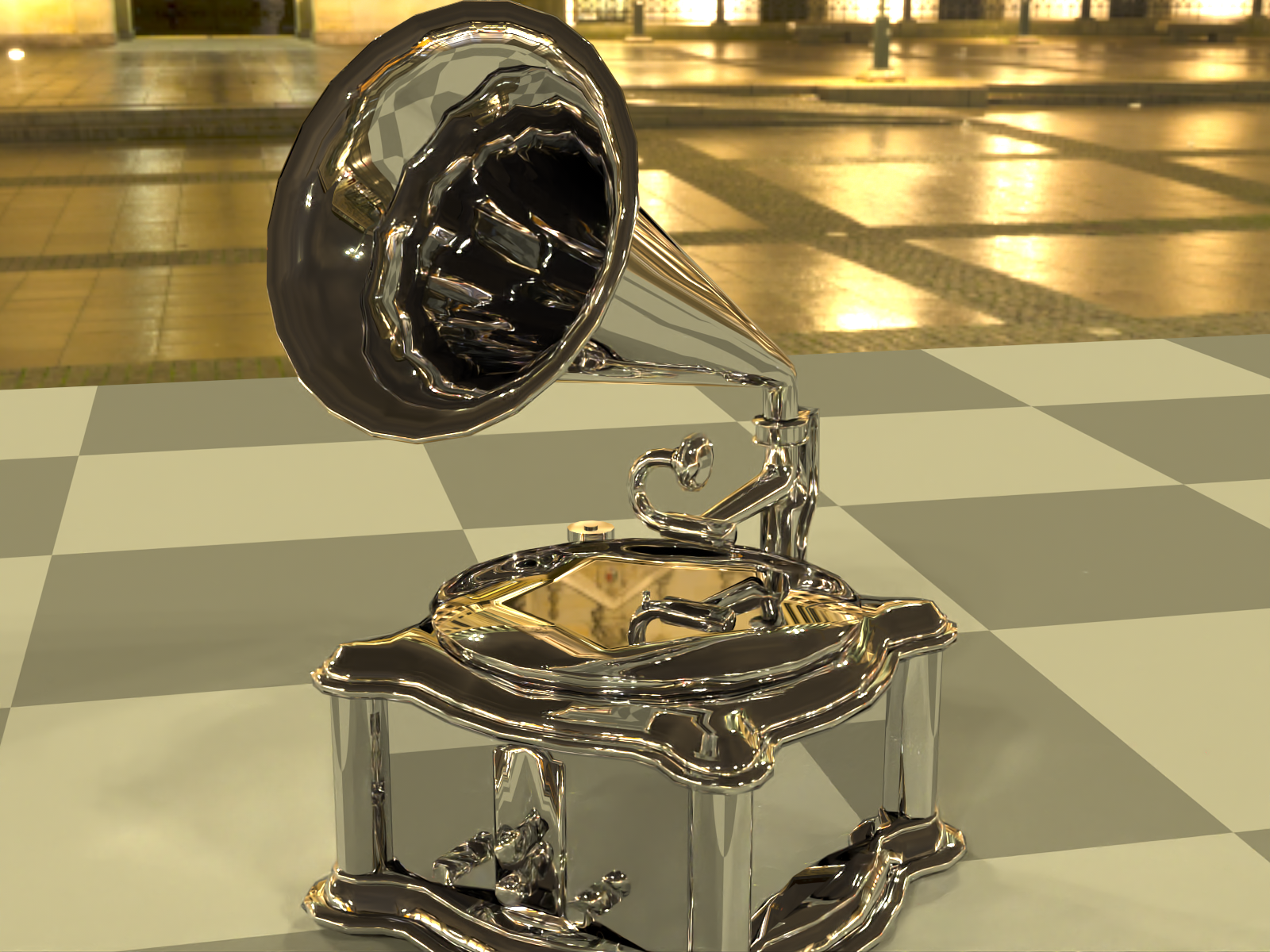
Conductor

Ground Truth 3DGS [74] InstantNGP [3]

Figure 6: Qualitative results for novel view synthesis.

Results and analysis. As shown in Tab. 2, the results for novel view synthesis highlight the same pattern as the 3D reconstruction ones, suggesting a commonality in how materials affect algorithm performance across different tasks and algorithms with varying principles. Specifically, the results indicate that materials such as Diffuse and Rough Plastic consistently yield the highest performance, while Conductor and Dielectric materials pose the greatest challenges. As in 3D reconstruction, the rough versions of these materials yield better results than their smooth counterparts.

Both Instant-NGP and Gaussian Splatting, which are fundamentally based on color consistency, excel with diffuse materials that adhere to this assumption. By contrast, the inherent high specular reflection and complex light transmission of Conductor and Dielectric materials disrupt multi-view color consistency, leading to chaotic color blocks in the rendered images. For example, in Fig. 6, the phonograph’s horn metal surface reflects the chessboard pattern on the ground, and both algorithms struggle to accurately reconstruct this specular reflection. Furthermore, for the chess piece, the background texture should appear by transparency, but both methods yield textures that are jumbled due to the color viewpoint dependency caused by transmission. Moreover, the sharp highlights due to reflections at the base are to some degree captured by Gaussian Splatting, whereas Instant-NGP fails to reconstruct these features.

Altogether, our results demonstrate that different novel view synthesis and 3D reconstruction algorithms exhibit consistent trends, underscoring that material properties represent a common challenge across these fields. This observation highlights the difficulties in accurately reconstructing materials with high specular and transparent characteristics, underscoring the necessity for developing algorithms that are specifically designed to handle complex materials.

5 Limitations and Conclusion

We have introduced OpenMaterial, the first large-scale dataset designed for quantitative assessment of 3D reconstruction methods for objects with complex materials, featuring an extensive variety of shapes, material types, and lighting conditions. Our dataset not only supports comprehensive evaluations but also facilitates the analysis of the capabilities of existing algorithms at handling challenging materials. We have validated its utility by evaluating state-of-the-art 3D reconstruction and novel view synthesis algorithms. The main limitation of our approach, however, lies in the dataset expansion. While it is theoretically possible to increase the variety of shapes by incorporating models from existing open-source datasets, the quality of many models does not meet real-world standards. This requires manual selection to ensure realism, a process that could become a bottleneck if demands for larger data volumes arise.

References

- [1] Z. Li, T. Müller, A. Evans, R. H. Taylor, M. Unberath, M.-Y. Liu, and C.-H. Lin, “Neuralangelo: High-fidelity neural surface reconstruction,” in Proceedings of the IEEE/CVF Conference on Computer Vision and Pattern Recognition, 2023, pp. 8456–8465.
- [2] L. Yariv, P. Hedman, C. Reiser, D. Verbin, P. P. Srinivasan, R. Szeliski, J. T. Barron, and B. Mildenhall, “Bakedsdf: Meshing neural sdfs for real-time view synthesis,” in ACM SIGGRAPH 2023 Conference Proceedings, 2023, pp. 1–9.
- [3] T. Müller, A. Evans, C. Schied, and A. Keller, “Instant neural graphics primitives with a multiresolution hash encoding,” ACM transactions on graphics (TOG), vol. 41, no. 4, pp. 1–15, 2022.
- [4] F. Wang, M.-J. Rakotosaona, M. Niemeyer, R. Szeliski, M. Pollefeys, and F. Tombari, “Unisdf: Unifying neural representations for high-fidelity 3d reconstruction of complex scenes with reflections,” arXiv preprint arXiv:2312.13285, 2023.
- [5] Y. Liu, P. Wang, C. Lin, X. Long, J. Wang, L. Liu, T. Komura, and W. Wang, “Nero: Neural geometry and brdf reconstruction of reflective objects from multiview images,” in SIGGRAPH, 2023.
- [6] K. Kutulakos and S. Seitz, “A theory of shape by space carving,” in Proceedings of the Seventh IEEE International Conference on Computer Vision, vol. 1, 1999, pp. 307–314 vol.1.
- [7] A. Fusiello, E. Trucco, and A. Verri, “A compact algorithm for rectification of stereo pairs,” Machine vision and applications, vol. 12, pp. 16–22, 2000.
- [8] R. Hartley and A. Zisserman, Multiple view geometry in computer vision. Cambridge university press, 2003.
- [9] M. Lhuillier and L. Quan, “A quasi-dense approach to surface reconstruction from uncalibrated images,” IEEE transactions on pattern analysis and machine intelligence, vol. 27, no. 3, pp. 418–433, 2005.
- [10] M. Goesele, B. Curless, and S. M. Seitz, “Multi-view stereo revisited,” in 2006 IEEE Computer Society Conference on Computer Vision and Pattern Recognition (CVPR’06), vol. 2. IEEE, 2006, pp. 2402–2409.
- [11] M. Kazhdan, M. Bolitho, and H. Hoppe, “Poisson surface reconstruction,” in Proceedings of the fourth Eurographics symposium on Geometry processing, vol. 7, no. 4, 2006.
- [12] S. Agarwal, Y. Furukawa, N. Snavely, I. Simon, B. Curless, S. M. Seitz, and R. Szeliski, “Building rome in a day,” Communications of the ACM, vol. 54, no. 10, pp. 105–112, 2011.
- [13] M. Bleyer, C. Rhemann, and C. Rother, “Patchmatch stereo-stereo matching with slanted support windows.” in Bmvc, vol. 11, 2011, pp. 1–11.
- [14] E. Tola, C. Strecha, and P. Fua, “Efficient large-scale multi-view stereo for ultra high-resolution image sets,” Machine Vision and Applications, vol. 23, pp. 903–920, 2012.
- [15] S. Shen, “Accurate multiple view 3d reconstruction using patch-based stereo for large-scale scenes,” IEEE transactions on image processing, vol. 22, no. 5, pp. 1901–1914, 2013.
- [16] J. L. Schonberger and J.-M. Frahm, “Structure-from-motion revisited,” in Proceedings of the IEEE conference on computer vision and pattern recognition, 2016, pp. 4104–4113.
- [17] C. B. Choy, D. Xu, J. Gwak, K. Chen, and S. Savarese, “3d-r2n2: A unified approach for single and multi-view 3d object reconstruction,” in Computer Vision–ECCV 2016: 14th European Conference, Amsterdam, The Netherlands, October 11-14, 2016, Proceedings, Part VIII 14. Springer, 2016, pp. 628–644.
- [18] C. Qi, H. Su, K. Mo, and L. Guibas, “Pointnet: Deep learning on point sets for 3d classification and segmentation,” in Conference on Computer Vision and Pattern Recognition, Honolulu, Hawaii, 2017.
- [19] S. Wang, R. Clark, H. Wen, and N. Trigoni, “Deepvo: Towards end-to-end visual odometry with deep recurrent convolutional neural networks,” in 2017 IEEE international conference on robotics and automation (ICRA). IEEE, 2017, pp. 2043–2050.
- [20] C. Tang and P. Tan, “Ba-net: Dense bundle adjustment network,” arXiv preprint arXiv:1806.04807, 2018.
- [21] Y. Yao, Z. Luo, S. Li, T. Fang, and L. Quan, “Mvsnet: Depth inference for unstructured multi-view stereo,” in Proceedings of the European conference on computer vision (ECCV), 2018, pp. 767–783.
- [22] R. Chen, S. Han, J. Xu, and H. Su, “Point-based multi-view stereo network,” in International Conference on Computer Vision, Seoul, Korea, 2019, pp. 1538–1547.
- [23] Y. Yao, Z. Luo, S. Li, T. Shen, T. Fang, and L. Quan, “Recurrent mvsnet for high-resolution multi-view stereo depth inference,” in Proceedings of the IEEE/CVF conference on computer vision and pattern recognition, 2019, pp. 5525–5534.
- [24] R. Chabra, J. Straub, C. Sweeney, R. Newcombe, and H. Fuchs, “Stereodrnet: Dilated residual stereonet,” in Proceedings of the IEEE/CVF conference on computer vision and pattern recognition, 2019, pp. 11 786–11 795.
- [25] H. Xu and J. Zhang, “Aanet: Adaptive aggregation network for efficient stereo matching,” in Proceedings of the IEEE/CVF conference on computer vision and pattern recognition, 2020, pp. 1959–1968.
- [26] B. Mildenhall, P. P. Srinivasan, M. Tancik, J. T. Barron, R. Ramamoorthi, and R. Ng, “Nerf: Representing scenes as neural radiance fields for view synthesis,” Communications of the ACM, vol. 65, no. 1, pp. 99–106, 2021.
- [27] D. Verbin, P. Hedman, B. Mildenhall, T. Zickler, J. T. Barron, and P. P. Srinivasan, “Ref-nerf: Structured view-dependent appearance for neural radiance fields,” in 2022 IEEE/CVF Conference on Computer Vision and Pattern Recognition (CVPR). IEEE, 2022, pp. 5481–5490.
- [28] J. T. Barron, B. Mildenhall, M. Tancik, P. Hedman, R. Martin-Brualla, and P. P. Srinivasan, “Mip-nerf: A multiscale representation for anti-aliasing neural radiance fields,” in Proceedings of the IEEE/CVF International Conference on Computer Vision, 2021, pp. 5855–5864.
- [29] J. T. Barron, B. Mildenhall, D. Verbin, P. P. Srinivasan, and P. Hedman, “Mip-nerf 360: Unbounded anti-aliased neural radiance fields,” in Proceedings of the IEEE/CVF Conference on Computer Vision and Pattern Recognition, 2022, pp. 5470–5479.
- [30] ——, “Zip-nerf: Anti-aliased grid-based neural radiance fields,” in Proceedings of the IEEE/CVF International Conference on Computer Vision, 2023, pp. 19 697–19 705.
- [31] L. Yariv, J. Gu, Y. Kasten, and Y. Lipman, “Volume rendering of neural implicit surfaces,” Advances in Neural Information Processing Systems, vol. 34, pp. 4805–4815, 2021.
- [32] P. Wang, L. Liu, Y. Liu, C. Theobalt, T. Komura, and W. Wang, “Neus: Learning neural implicit surfaces by volume rendering for multi-view reconstruction,” arXiv preprint arXiv:2106.10689, 2021.
- [33] Z. Yu, S. Peng, M. Niemeyer, T. Sattler, and A. Geiger, “Monosdf: Exploring monocular geometric cues for neural implicit surface reconstruction,” Advances in neural information processing systems, vol. 35, pp. 25 018–25 032, 2022.
- [34] Y. Wang, I. Skorokhodov, and P. Wonka, “Hf-neus: Improved surface reconstruction using high-frequency details,” Advances in Neural Information Processing Systems, vol. 35, pp. 1966–1978, 2022.
- [35] Y. Wang, Q. Han, M. Habermann, K. Daniilidis, C. Theobalt, and L. Liu, “Neus2: Fast learning of neural implicit surfaces for multi-view reconstruction,” in Proceedings of the IEEE/CVF International Conference on Computer Vision (ICCV), 2023.
- [36] K. Gao, Y. Gao, H. He, D. Lu, L. Xu, and J. Li, “Nerf: Neural radiance field in 3d vision, a comprehensive review,” arXiv preprint arXiv:2210.00379, 2022.
- [37] D. Wang, T. Zhang, and S. Süsstrunk, “Nemto: Neural environment matting for novel wiew and relighting synthesis of transparent objects,” in Proceedings of the IEEE/CVF International Conference on Computer Vision, 2023, pp. 317–327.
- [38] M. Boss, R. Braun, V. Jampani, J. T. Barron, C. Liu, and H. Lensch, “Nerd: Neural reflectance decomposition from image collections,” in Proceedings of the IEEE/CVF International Conference on Computer Vision, 2021, pp. 12 684–12 694.
- [39] Z. Kuang, K. Olszewski, M. Chai, Z. Huang, P. Achlioptas, and S. Tulyakov, “Neroic: Neural rendering of objects from online image collections,” ACM Trans. Graph., vol. 41, no. 4, jul 2022. [Online]. Available: https://doi.org/10.1145/3528223.3530177
- [40] M. Toschi, R. D. Matteo, R. Spezialetti, D. D. Gregorio, L. D. Stefano, and S. Salti, “Relight my nerf: A dataset for novel view synthesis and relighting of real world objects,” in 2023 IEEE/CVF Conference on Computer Vision and Pattern Recognition (CVPR). Los Alamitos, CA, USA: IEEE Computer Society, jun 2023, pp. 20 762–20 772. [Online]. Available: https://doi.ieeecomputersociety.org/10.1109/CVPR52729.2023.01989
- [41] I. Liu, L. Chen, Z. Fu, L. Wu, H. Jin, Z. Li, C. M. R. Wong, Y. Xu, R. Ramamoorthi, Z. Xu et al., “Openillumination: A multi-illumination dataset for inverse rendering evaluation on real objects,” Advances in Neural Information Processing Systems, vol. 36, 2024.
- [42] B. Mildenhall, P. P. Srinivasan, R. Ortiz-Cayon, N. K. Kalantari, R. Ramamoorthi, R. Ng, and A. Kar, “Local light field fusion: Practical view synthesis with prescriptive sampling guidelines,” ACM Transactions on Graphics (TOG), vol. 38, no. 4, pp. 1–14, 2019.
- [43] G. Oxholm and K. Nishino, “Multiview shape and reflectance from natural illumination,” in Proceedings of the IEEE Conference on Computer Vision and Pattern Recognition, 2014, pp. 2155–2162.
- [44] H. Aanæs, R. R. Jensen, G. Vogiatzis, E. Tola, and A. B. Dahl, “Large-scale data for multiple-view stereopsis,” International Journal of Computer Vision, vol. 120, pp. 153–168, 2016.
- [45] A. Knapitsch, J. Park, Q.-Y. Zhou, and V. Koltun, “Tanks and temples: Benchmarking large-scale scene reconstruction,” ACM Transactions on Graphics, vol. 36, no. 4, 2017.
- [46] M. Li, Z. Zhou, Z. Wu, B. Shi, C. Diao, and P. Tan, “Multi-view photometric stereo: A robust solution and benchmark dataset for spatially varying isotropic materials,” IEEE Transactions on Image Processing, vol. 29, pp. 4159–4173, 2020.
- [47] Z. Kuang, Y. Zhang, H.-X. Yu, S. Agarwala, S. Wu, and J. Wu, “Stanford-orb: A real-world 3d object inverse rendering benchmark,” 2023.
- [48] T. Wu, J. Zhang, X. Fu, Y. Wang, L. P. Jiawei Ren, W. Wu, L. Yang, J. Wang, C. Qian, D. Lin, and Z. Liu, “Omniobject3d: Large-vocabulary 3d object dataset for realistic perception, reconstruction and generation,” in IEEE/CVF Conference on Computer Vision and Pattern Recognition (CVPR), 2023.
- [49] V. Jampani, K.-K. Maninis, A. Engelhardt, A. Karpur, K. Truong, K. Sargent, S. Popov, A. Araujo, R. Martin Brualla, K. Patel et al., “Navi: Category-agnostic image collections with high-quality 3d shape and pose annotations,” Advances in Neural Information Processing Systems, vol. 36, 2024.
- [50] J. Shi, Y. Dong, H. Su, and S. X. Yu, “Learning non-lambertian object intrinsics across shapenet categories,” in Proceedings of the IEEE conference on computer vision and pattern recognition, 2017, pp. 1685–1694.
- [51] Y. Yao, Z. Luo, S. Li, J. Zhang, Y. Ren, L. Zhou, T. Fang, and L. Quan, “Blendedmvs: A large-scale dataset for generalized multi-view stereo networks,” Computer Vision and Pattern Recognition (CVPR), 2020.
- [52] M. Deitke, D. Schwenk, J. Salvador, L. Weihs, O. Michel, E. VanderBilt, L. Schmidt, K. Ehsani, A. Kembhavi, and A. Farhadi, “Objaverse: A universe of annotated 3d objects,” in Proceedings of the IEEE/CVF Conference on Computer Vision and Pattern Recognition, 2023, pp. 13 142–13 153.
- [53] J. Collins, S. Goel, K. Deng, A. Luthra, L. Xu, E. Gundogdu, X. Zhang, T. F. Y. Vicente, T. Dideriksen, H. Arora et al., “Abo: Dataset and benchmarks for real-world 3d object understanding,” in Proceedings of the IEEE/CVF Conference on Computer Vision and Pattern Recognition, 2022, pp. 21 126–21 136.
- [54] B. Walter, S. R. Marschner, H. Li, and K. E. Torrance, “Microfacet models for refraction through rough surfaces,” in Proceedings of the 18th Eurographics conference on Rendering Techniques, 2007, pp. 195–206.
- [55] M. Born and E. Wolf, Principles of optics: electromagnetic theory of propagation, interference and diffraction of light. Elsevier, 2013.
- [56] P. B. Johnson and R. W. Christy, “Optical constants of the noble metals,” Phys. Rev. B, vol. 6, pp. 4370–4379, Dec 1972. [Online]. Available: https://link.aps.org/doi/10.1103/PhysRevB.6.4370
- [57] A. D. Rakić, “Algorithm for the determination of intrinsic optical constants of metal films: application to aluminum,” Applied optics, vol. 34, no. 22, pp. 4755–4767, 1995.
- [58] A. Bideau-Mehu, Y. Guern, R. Abjean, and A. Johannin-Gilles, “Measurement of refractive indices of neon, argon, krypton and xenon in the 253.7–140.4 nm wavelength range. dispersion relations and estimated oscillator strengths of the resonance lines,” Journal of Quantitative Spectroscopy and Radiative Transfer, vol. 25, no. 5, pp. 395–402, 1981.
- [59] P. Johnson and R. Christy, “Optical constants of transition metals: Ti, v, cr, mn, fe, co, ni, and pd,” Physical review B, vol. 9, no. 12, p. 5056, 1974.
- [60] N. V. Smith, “Optical constants of rubidium and cesium from 0.5 to 4.0 ev,” Physical Review B, vol. 2, no. 8, p. 2840, 1970.
- [61] T. Inagaki, E. Arakawa, and M. Williams, “Optical properties of liquid mercury,” Physical review B, vol. 23, no. 10, p. 5246, 1981.
- [62] M. Fernández-Perea, J. I. Larruquert, J. A. Aznárez, J. A. Méndez, L. Poletto, F. Frassetto, A. M. Malvezzi, D. Bajoni, A. Giglia, N. Mahne et al., “Transmittance and optical constants of ho films in the 3–1340 ev spectral range,” Journal of Applied Physics, vol. 109, no. 8, 2011.
- [63] I. H. Malitson and M. J. Dodge, “Refractive index and birefringence of synthetic sapphire,” J. Opt. Soc. Am, vol. 62, no. 11, p. 1405, 1972.
- [64] I. H. Malitson, “Refractive properties of barium fluoride,” JOSA, vol. 54, no. 5, pp. 628–632, 1964.
- [65] E. D. Palik, Handbook of optical constants of solids. Academic press, 1998, vol. 3.
- [66] M. Simon, F. Mersch, C. Kuper, S. Mendricks, S. Wevering, J. Imbrock, and E. Krätzig, “Refractive indices of photorefractive bismuth titanate, barium-calcium titanate, bismuth germanium oxide, and lead germanate,” physica status solidi (a), vol. 159, no. 2, pp. 559–562, 1997.
- [67] S.-Y. Lee, T.-Y. Jeong, S. Jung, and K.-J. Yee, “Refractive index dispersion of hexagonal boron nitride in the visible and near-infrared,” physica status solidi (b), vol. 256, no. 6, p. 1800417, 2019.
- [68] X. Zhang, J. Qiu, X. Li, J. Zhao, and L. Liu, “Complex refractive indices measurements of polymers in visible and near-infrared bands,” Applied optics, vol. 59, no. 8, pp. 2337–2344, 2020.
- [69] I. Bodurov, I. Vlaeva, A. Viraneva, T. Yovcheva, and S. Sainov, “Modified design of a laser refractometer,” Nanosci. Nanotechnol, vol. 16, pp. 31–33, 2016.
- [70] M. R. Querry, Optical constants of minerals and other materials from the millimeter to the ultraviolet. Chemical Research, Development & Engineering Center, US Army Armament …, 1998.
- [71] N. Sultanova, S. Kasarova, and I. Nikolov, “Dispersion properties of optical polymers,” Acta Physica Polonica A, vol. 116, no. 4, pp. 585–587, 2009.
- [72] M. N. Polyanskiy, “Refractiveindex. info database of optical constants,” Scientific Data, vol. 11, no. 1, p. 94, 2024.
- [73] W. Jakob, S. Speierer, N. Roussel, and D. Vicini, “Dr.jit: A just-in-time compiler for differentiable rendering,” Transactions on Graphics (Proceedings of SIGGRAPH), vol. 41, no. 4, Jul. 2022.
- [74] B. Kerbl, G. Kopanas, T. Leimkühler, and G. Drettakis, “3d gaussian splatting for real-time radiance field rendering,” ACM Transactions on Graphics, vol. 42, no. 4, July 2023. [Online]. Available: https://repo-sam.inria.fr/fungraph/3d-gaussian-splatting/
- [75] Y.-C. Guo, “Instant neural surface reconstruction,” 2022, https://github.com/bennyguo/instant-nsr-pl.