IMFL-AIGC: Incentive Mechanism Design for Federated Learning Empowered by Artificial Intelligence Generated Content

Abstract

Federated learning (FL) has emerged as a promising paradigm that enables clients to collaboratively train a shared global model without uploading their local data. To alleviate the heterogeneous data quality among clients, artificial intelligence-generated content (AIGC) can be leveraged as a novel data synthesis technique for FL model performance enhancement. Due to various costs incurred by AIGC-empowered FL (e.g., costs of local model computation and data synthesis), however, clients are usually reluctant to participate in FL without adequate economic incentives, which leads to an unexplored critical issue for enabling AIGC-empowered FL. To fill this gap, we first devise a data quality assessment method for data samples generated by AIGC and rigorously analyze the convergence performance of FL model trained using a blend of authentic and AI-generated data samples. We then propose a data quality-aware incentive mechanism to encourage clients’ participation. In light of information asymmetry incurred by clients’ private multi-dimensional attributes, we investigate clients’ behavior patterns and derive the server’s optimal incentive strategies to minimize server’s cost in terms of both model accuracy loss and incentive payments for both complete and incomplete information scenarios. Numerical results demonstrate that our proposed mechanism exhibits highest training accuracy and reduces up to $53.34\%$ of the server’s cost with real-world datasets, compared with existing benchmark mechanisms.

I Introduction

The fast proliferation of edge devices (e.g., mobile devices and wearable devices) in modern society has led to the rapid growth of data generated from massive distributed sources, which further promotes the advancement of a wide range of artificial intelligent applications (e.g., autonomous driving and healthcare) [1, 2]. However, due to the increasing privacy concerns [3] and limited network bandwidth, the predominant mechanism that gathers extensive data from dispersed devices to the cloud for centralized model training becomes impractical. To reap the benefits of the scattered data without privacy risk, federated learning (FL) [4] has emerged as a promising paradigm that enables to collaboratively train a shared global model by aggregating locally-computed updates uploaded by clients (e.g., mobile devices). By decoupling model training from the need of direct access of the local data on the devices, FL realizes distributed and privacy-preserving model training.

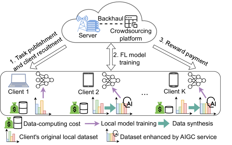
Figure 1: AIGC-empowered federated learning scenario.

Nevertheless, most existing FL frameworks usually make an optimistic assumption that clients participate in FL model training voluntarily and ignore the inevitable data-computing cost (e.g., battery and CPU resource consumption for local model updates) incurred by inevitable training [5], [6]. While in reality, rational clients would be reluctant to participate in model training without sufficient economic compensation [7], [8]. By paying rewards to compensate the cost of clients reasonably, incentive mechanism has garnered significant attention from researchers and become the essential financial catalyst for making FL a reality [9].

Despite the promising benefits of privacy preservation, federated learning performance remains constrained in mobile application scenarios due to challenges such as non-IID (a.k.a. non independent and identically distributed) nature of data from scattered mobile devices [10]. In certain mobile applications, such as autonomous vehicle training [11], [12] and health monitoring [13], the lack of specific labeled data further exacerbates this issue, as the characteristics of users’ datasets vary according to their activities. To alleviate the issue of non-IID data distribution and data scarcity inherent in FL, the great explosion of artificial intelligence-generated content (AIGC) service [14] has opened up a compelling avenue for the clients to generate high-quality data (e.g., images and videos) with generative AI techniques at a rapid pace. For example, by leveraging generative adversarial networks, clients are able to collectively train a generative model to augment their local data towards yielding an IID dataset [15]. Empowered with generative AI services (e.g., Stable Diffusion [16]), the learning performance of FL can be significantly improved by utilizing a pre-trained diffusion model to synthesize customized local data [17]. Consequently, integrating AIGC as a data synthesis tool at the client side can substantially improve data quality and enhance FL model performance in real-world applications.

However, the additional costs of data generation by AIGC service would mitigate clients’ willingnesses to participate in federated learning without sufficient economic compensation, thereby presenting new challenges to current incentive mechanisms which does not consider the complex clients’ behaviors on whether to adopt AIGC service [10], [17], [18]. In light of potential benefits and challenges of using AIGC technique in the context of FL, it is non-trivial to devise efficient incentive mechanism for such a complicated AIGC-empowered FL scenario to encourage clients to contribute their data (e.g., local data or rectified data by AIGC service) and resources for FL model training while minimizing server’s own cost (e.g., payments for client recruiting, model accuracy loss, etc.). First, an indispensable preliminary step for effective incentive mechanism involves performance assessment of the final converged model prior to commencing FL model training. As the model performance is jointly influenced by many factors, i.e., the number of global training iterations, clients’ attributes including the quantity and quality of the local data, it is non-trivial to evaluate the final model performance [19, 20]. Moreover, the data quality changes resulted from clients’ adoption of AIGC service for data synthesis presents key challenges for model performance evaluation. Second, faced the temptation of being rewarded, clients may choose to generate a high-quality dataset by leveraging AIGC service (e.g., reaching IID dataset by replenishing data samples in minority classes) for local model updates, which may further affect the server’s decision-making regarding client recruitment, and hence make the design of optimal incentive strategy much more involved. Third, clients’ individual attributes (e.g., data quality and data-computing cost) also bring difficulty to the incentive mechanism design due to information asymmetry (i.e., such private client’s information may not be available to the server for decision making prior to the FL training process).

To overcome the aforementioned challenges, in this paper, we propose a data quality-aware incentive mechanism in AIGC-empowered FL scenario. As illustrated in Fig. 1, the server publishes a training task and encourages clients’ participation through a crowdsourcing platform (e.g., Amazon Mechanical Turk) with a data quality-aware reward allocation mechanism. By analyzing the convergence performance bound in AIGC-empowered FL scenario, we formulate the server’s cost in terms of model accuracy loss and payment to clients. Furthermore, we reveal server’s optimal incentive strategy to minimize its cost by fully studying clients’ rational behaviors under different information settings (i.e., complete and incomplete information scenarios).

In summary, this paper makes the following contributions:

• Incentive mechanism design for AIGC-empowered FL. We first devise a data quality assessment method for data samples generated by AIGC and then propose a data quality-aware incentive mechanism to encourage clients’ participation. By characterizing the clients’ complex behavior patterns (e.g., whether to participate in FL, whether to use generated data samples), we design a data quality-aware reward allocation mechanism for the participating clients and derive the server’s optimal incentive strategy. To the best of our knowledge, this is the first paper to study the incentive mechanism design for AIGC-empowered FL.

• Analysis of model training performance for AIGC-empowered FL. We derive a novel convergence upper bound of the gap between FL model training loss and the optimal loss value in AIGC-empowered FL scenarios where clients may choose to adopt AIGC-enhanced dataset for local model training instead of their original local dataset.

• Investigation on the impact of information asymmetry and the adoption of AIGC service. Compared with complete information scenario, the server may suffer from high cost to hedge the risk of no or very few clients participating in FL model training in incomplete information scenario. Hence, the server tends to boost the incentive reward especially in the case with a small number of candidate clients. Facing with small candidate client size of lower data quality, the adoption of AIGC service for data sysnthesis can bring a much more significant gain in server’s cost reduction for both complete and incomplete information scenarios.

• Performance evaluation. Extensive performance evaluations based on real-world datasets validate our theoretical analysis and show that our incentive mechanism exhibits superior performance, e.g., achieving up-to 53.34% server’s cost reduction and highest training accuracy, compared with the benchmark mechanisms.

II System Model

In this section, we first introduce AIGC-empowered FL paradigm. We further characterize clients’ attributes, clients’ utility functions and server’s utility function. Finally, we propose data quality-aware incentive mechanism under complete and incomplete information scenarios. For readability, we summarize the key notations in Table I.

II-A AIGC-empowered Federated Learning

As illustrated in Fig. 1, we consider a AIGC-empowered FL scenario, which comprises of one server and a set $\mathcal{K}=\{1,...,K\}$ of candidate clients who can choose to leverage AIGC service for high-quality data synthesis. As a result, each client can participate in FL with its original local dataset $\mathcal{D}_{k}$ or AIGC-enhanced dataset $\mathcal{D}_{k}^{A}$ aided with data synthesis.

TABLE I: List of key notations.

Symbol	Description
$\mathcal{K}$	The set of candidate clients
$\mathcal{D}_{k}$	Local dataset of client $k$
$\mathcal{D}_{k}^{A}$	AIGC-enhanced dataset of client $k$
$F_{k,L}$	Loss function of client $k$ over its local dataset
$F_{k,A}$	Loss function for client $k$ over its AIGC-enhanced dataset
$p^{k}_{a}(y=i)$	Client $k$ ’s proportion of data samples for data synthesis
$d_{k}$	Data size of client $k$
$\lambda_{k}$	Parameter for data quality of client $k$’s local dataset
$\lambda_{k,A}$	Parameter for data quality of client $k$’s AIGC-enhanced dataset
$s_{k}$	Data-computing cost per unit data sample for client $k$
$\mathcal{N}$	The set of participating clients
$\mathcal{N}^{L}$	The set of participating clients using local datasets
$\mathcal{N}^{A}$	The set of participating clients using AIGC-enhanced datasets
$r$	The uniform unit data reward benchmark $r$
$T$	The number of global iterations
$R(\mathcal{N}_{r})$	Total payment to participating clients given benchmark $r$

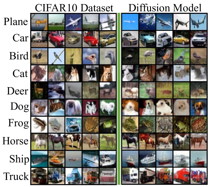
Figure 2: Comparison between real-world data samples and generated data samples.

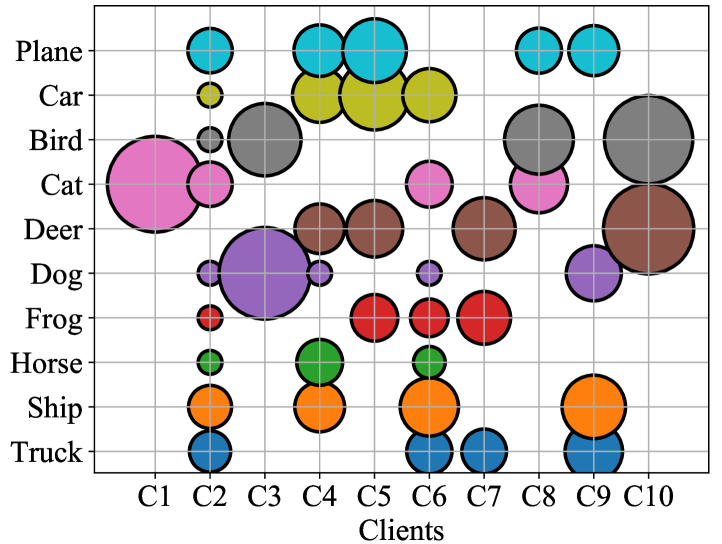
Figure 3: Distribution among classes of the local datasets for 10 randomly selected clients.

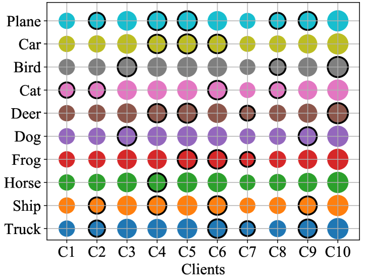
Figure 4: Distribution among classes of the AIGC-enhanced dataset for 10 randomly selected clients.

For a general classification task, each data sample $(\bm{x},y)$ in the local dataset $\mathcal{D}_{k}$ distributes over $\mathcal{X}\times\mathcal{Y}$ following the distribution $\bm{p}$ [21], where $\mathcal{X}$ is a compact space of data features $\bm{x}$ and $\mathcal{Y}=\{1,...,Y\}$ represents the label space for ground-truth $y$. The number of total data samples of client $k$ is denoted as $d_{k}$. To conduct model training, a function (e.g., neural network) $f(\bm{x})=(f_{1}(\bm{x}),...,f_{Y}(\bm{x})):\mathcal{X}\rightarrow\mathcal{M}$ parameterized over the hypothesis class $\bm{w}$ is employed. Here, $f_{i}(\bm{x})$ quantifies the probability of data sample $(\bm{x},y)$ belonging to the $i$-th class and $\mathcal{M}=\{(m_{1},...,m_{Y})|\sum_{i\in\mathcal{Y}}m_{i}=1,m_{i}\geq 0,\forall i\in\mathcal{Y}\}$. The loss function for client $k$ over its local dataset $\mathcal{D}_{k}$ can be defined with the widely-used cross-entropy loss as:

$$F_{k,L}(\bm{w})=\mathbb{E}_{\bm{x},y\sim\bm{p}}\left[\sum_{i=1}^{Y}-p^{k}(y=i)\log f_{i}(\bm{w};\bm{x})\right]$$

$$=\sum_{i=1}^{Y}p^{k}(y=i)\mathbb{E}_{x|y=i}\ell_{i}(\bm{w};\bm{x}),$$ (1)

where $\ell_{i}(\bm{w};\bm{x})=-\log f_{i}(\bm{w};\bm{x})$. $p^{k}(y=i)$ denotes the proportion of data samples belonging to the $i$-th class in $\mathcal{D}_{k}$. Accordingly, the goal of FL is to minimize a global loss function, a weighted average of loss functions of all clients, i.e., $\min_{\bm{w}}F(\bm{w})=\sum_{k\in\mathcal{K}}\frac{d_{k}}{d(\mathcal{K})}F_{k}(\bm{w})$, where $d(\mathcal{K})=\sum_{k\in\mathcal{K}}d_{k}$ is the total number of data samples of all clients in $\mathcal{K}$.

Moreover, each client $k\in\mathcal{K}$ can also conduct data synthesis by adopting AIGC service (e.g., Dall-E or Stable Diffusion) to obtain a higher-quality AIGC-enhanced dataset $\mathcal{D}_{k}^{A}$, which is a mixture of local real-world data samples and generated data samples under IID data distribution. As an illustration, we utilize diffusion model [22] to mimic the provisioning of AIGC service for the clients due to its impressive capability in generating photo-realistic images with rich texture as shown in Fig. 4. For client $k$ with non-IID data distribution, the data synthesis process is performed as follows: for each class $i$, given the proportion of data samples with class $i$ in the global data (denoted as $p(y=i)$) and the proportion of data samples with class $i$ in $\mathcal{D}_{k}$ (denoted as $p^{k}(y=i)$), the proportion of data samples for data synthesis is calculated as $p^{k}_{a}(y=i)=p(y=i)-p^{k}(y=i)$. For simplicity, we adopt this data synthesis process by keeping the datasize $d_{k}$ unchanged , i.e., $|\mathcal{D}^{A}_{k}|=|\mathcal{D}_{k}|=d_{k}$. Hence, $p^{k}_{a}(y=i)>0$ indicates that client $k$ generates $p^{k}_{a}(y=i)d_{k}$ data samples with label $i$ by utilizing AIGC service. While client $k$ removes the redundant $p^{k}_{a}(y=i)d_{k}$ data samples with label $i$ from its local dataset when $p^{k}_{a}(y=i)\leq 0$. As depicted in Fig. 4, we randomly select 10 clients with non-IID data distributions, the area of a circle represents the amount of data samples for a target class. By conducting data synthesis discussed above, we replenish data samples for the minority classes (circles without black borders as depicted in Fig. 4) and obtain higher-quality (e.g., more IID) AIGC-enhanced datasets for each client.

We assume that each generated data sample distributes over $\mathcal{X}\times\mathcal{Y}$ following distribution $\bm{p}_{a}$. By obtaining the definitions of $f_{i,a}(\bm{w};\bm{x})$ and $\ell_{i,a}(\bm{w};\bm{x})$ which are similar with $f_{i}(\bm{w};\bm{x})$ and $\ell_{i}(\bm{w};\bm{x})$, respectively, we define the loss function for client $k$ over its AIGC-enhanced dataset $\mathcal{D}_{k}^{A}$ as:

$$F_{k,A}(\bm{w})= \!\!\!\!\!\!\!\!\!\sum_{i\in\mathcal{I}_{k}}p^{k}_{a}(y=i)\mathbb{E}_{x|y=i}\ell_{i,a}(\bm{w};\bm{x})$$ (2)

$$\!\!\!\!\!\!\!\!\!\!+\sum_{i\notin\mathcal{I}_{k}}p(y=i)\mathbb{E}_{x|y=i}\ell_{i}(\bm{w};\bm{x}),$$

where $\mathcal{I}_{k}=\{i|i\in\mathcal{Y},p_{a}^{k}(y=i)>0\}$ denotes the set of labels injected by generated data samples for client $k$.

To reap the benefits from clients’ local (or AIGC-enhanced) dataset, we adopt the widely-accepted synchronous FL paradigm, which entails multiple iterations between the server and clients for global model training until reaching a predetermined global iteration numbers $T$. Specifically, each iteration consists of both local model training process and global model aggregation process as follows:

1) Local model training on $\mathcal{D}_{k}$ or $\mathcal{D}_{k}^{A}$: The server incentivizes a set of clients $\mathcal{N}\subset\mathcal{K}$ to participate in FL. In each global iteration $t$, each client $k\in\mathcal{N}$ receives current global model $\bm{w}^{t-1}$ from the server and conducts $h$-step local updates based on $\bm{w}^{t-1}$ through mini-batch stochastic gradient descent (SGD) algorithm over its local or AIGC-enhanced dataset. For ease of presentation, we denote $\bm{w}_{k}(t,t_{l})$ as local model of client $k$ at $(t_{l}-(t-1)h)$-th step in global iteration $t$. Here, $t_{l}\in((t-1)h,th]$ represents the $t_{l}$-th local update starting from the beginning of global model training. According to the definition, the model parameters of client $k$ evolve as:

$$\bm{w}_{k}(t,t_{l})=\left\{\begin{aligned} &\bm{w}_{k}(t,t_{l}-1)-\eta\nabla F_{k}(\bm{w}_{k}(t,t_{l}-1);\bm{\xi}_{k}^{t,t_{l}}),\\ &\quad\qquad\qquad\qquad\qquad\qquad\mbox{if}\ t_{l}\!\!\!\!\!\mod h\!\neq\!0,\\ &\bm{w}(t,t_{l}),\ \mbox{if}\ t_{l}\!\!\!\mod h=0,\end{aligned}\right.$$ (3)

where

$$\!\!\!\!\!\!\!\bm{w}(t,t_{l})=\sum_{k\in\mathcal{N}}\!\!\frac{d_{k}\!\!\left[\bm{w}_{k}(t,t_{l}\!-\!1)\!-\!\eta\nabla F_{k}(\bm{w}_{k}(t,t_{l}\!-\!1);\bm{\xi}_{k}^{t,t_{l}})\right]}{d(\mathcal{N})}.\!\!\!\!\!\!\!\!\!\!\!\!\!\!\!\!\!\!\!\!\!\!\!\!$$

Here, $\nabla F_{k}(\bm{w}_{k}(t,t_{l}-1);\bm{\xi}_{k}^{t,t_{l}})$ denotes the gradient of client $k$ and $\bm{\xi}_{k}^{t,t_{l}}$ represents the mini-batch data samples. For ease of presentation, we have $\nabla F_{k}(\bm{w}_{k}(t,t_{l}-1);\bm{\xi}_{k}^{t,t_{l}})=\nabla F_{k,L}(\bm{w}_{k}(t,t_{l}-1);\bm{\xi}_{k,L}^{t,t_{l}})$ for local dataset and $\nabla F_{k}(\bm{w}_{k}(t,t_{l}-1);\bm{\xi}_{k}^{t,t_{l}})=\nabla F_{k,A}(\bm{w}_{k}(t,t_{l}-1);\bm{\xi}_{k,A}^{t,t_{l}})$ for AIGC-enhanced dataset. Accordingly, we have $\bm{\xi}_{k}^{t,t_{l}}=\bm{\xi}_{k,L}^{t,t_{l}}$ for local dataset and $\bm{\xi}_{k}^{t,t_{l}}=\bm{\xi}_{k,A}^{t,t_{l}}$ for AIGC-enhanced dataset. In this paper, we adopt a widely-used FL setting that the batchsize $B_{k}$ of each client $k$ is in the same proportion to its data size by setting $d_{k}=hB_{k}$ [23, 24, 25]. After $h$-step local updates, each client $k$ uploads its local model to the server.

2) Global model aggregation: At global iteration $t$, the server receives all local models from client set $\mathcal{N}$, and conducts model aggregation to obtain a new global model $\bm{w}^{t}=\bm{w}(t,t_{l})$ where $t_{l}\mod h=0$.

II-B Client’s Attributes

Clients in FL scenarios greatly vary in device usage patterns (due to diverse physical characteristics and behavioral habits of users) and computation resource budgets (including computation capacity, memory, etc.), which results in diverse data-computing cost, data amounts and distributions among clients, and further affects FL model training performance, Hence, we identify each client $k$ by a tuple of attributes $\langle d_{k},\lambda_{k},s_{k}\rangle$, each of which is characterized as follows:

II-B1 Data quality of local and AIGC-enhanced datasets

We adopt $\|\nabla F_{k,L}(\bm{w})-\nabla F(\bm{w})\|\leq\lambda_{k}$ for any $\bm{w}$ to characterize the data quality of client $k\in\mathcal{K}$, where $\lambda_{k}$ is defined as the upper bound of the gradient difference between the local loss function and the global loss function [26], with larger $\lambda_{k}$ being poorer data quality. Specifically, $\lambda_{k}$ can be estimated by the widely-adopted average earth mover’s distance (EMD), which measures the data distribution heterogeneity (e.g., non-IID degree) among clients [21], i.e.,

$$\|\nabla F_{k,L}(\bm{w})-\nabla F(\bm{w})\|$$ (5)

$$= \|\sum_{i=1}^{Y}[p^{k}(y=i)-p(y=i)]\nabla\mathbb{E}_{x|y=i}\ell_{i}(x,\bm{w})\|$$

$$\leq \sum_{i=1}^{Y}\|p^{k}(y=i)-p(y=i)\|\|\mathbb{E}_{x|y=i}\ell_{i}(x,\bm{w})\|$$

$$\leq EMD_{k}\cdot g_{data}=\lambda_{k},$$

where $EMD_{k}=\sum_{i=1}^{Y}\|p^{k}(y=i)-p(y=i)\|$ and $g_{data}=\max_{i\in\mathcal{Y}}\|\mathbb{E}_{x|y=i}\ell_{i}(x,\bm{w})\|$ for any $\bm{w}$.

According to the definition in (2), the data quality of AIGC-enhanced dataset $\mathcal{D}_{k}^{A}$ can be characterized by $\lambda_{k,A}$, which is defined as the upper bound of the gradient difference between the loss function calculated based on the AIGC-enhanced dataset and the global loss function:

$$\|\nabla F_{k,A}(\bm{w})-\nabla F(\bm{w})\|$$ (6)

$$\leq \sum_{i\in\mathcal{I}_{k}}p_{a}^{k}(y=i)\|\nabla\mathbb{E}_{x|y=i}\ell_{i,a}(\bm{w};\bm{x})-\nabla\mathbb{E}_{x|y=i}\ell_{i}(\bm{w};\bm{x})\|$$

$$\leq \frac{EMD_{k}}{2}\cdot g_{diff}=\lambda_{k,A},$$

where $g_{diff}=max_{i\in\mathcal{Y}}\|\nabla\mathbb{E}_{x|y=i}\ell_{i,a}(\bm{w};\bm{x})-\nabla\mathbb{E}_{x|y=i}\ell_{i}(\bm{w};\bm{x})\|$, for any $\bm{w}$, which characterizes the maximum gradient error between generated and real-world data samples among all classes. Intuitively, a lower $g_{diff}$ indicates that distribution of the generated data is more similar to real-world data, i.e., higher generated data quality.

Based on the above discussions, we construct the relationship of the data quality between local dataset and AIGC-enhanced dataset for client $k$ based on the upper bounds, i.e.,

$$\lambda_{k,A}=\theta\lambda_{k},$$ (7)

where $\theta=\frac{g_{diff}}{2g_{data}}$, and it is a constant given a fixed FL task and AIGC model. In reality, the data quality of AIGC-enhanced dataset still depends on performance of AIGC model. We utilize $\theta$ to characterize the difference of data distribution between generated data samples (e.g., $\bm{p}_{a}$) and real-world data samples (e.g., $\bm{p}$). A lower $\theta$ indicates higher performance of generated data samples by AIGC (approaching data distribution of real-world data). Intuitively, $\theta<1$ means that introducing generated data can improve the data quality for each client . Compared with the data quality of an IID dataset only involving generated samples $g_{diff}$, the AIGC-enhanced dataset $\mathcal{D}_{k}^{A}$ possess higher data quality since $\lambda_{k,A}<g_{diff}$.

Remark 1: In practice, the server can publish a small-scale public dataset (SPD) with IID data distribution on the crowd-sourcing platform, and then the value of $\lambda_{k}$ can be estimated by a client $k$ through recording the gradient differences on the initial model between its local dataset and the SPD as a testing process of model training. Besides, $g_{data}$ can be estimated by recording maximum gradient norm based on the initial model for each class in SPD. The generated data quality $g_{diff}$ can be determined by recording the maximum gradient error for each class between samples in SPD and generated data samples by AIGC service. Then, parameter $\theta$ can be determined, which can be regarded as the consensus of all clients and the server.

II-B2 Data-computing cost

We denote the data-computing cost per unit data sample by $s_{k}$. As each client $k$ conducts $h$-step local updates with mini-batch size $B_{k}=\frac{d_{k}}{h}$ in one global iteration in our settings, the data-computing cost for local model training of client $k$ can be calculated as $d_{k}s_{k}$ in one global iteration. We assume that the stochastic gradient is unbiased and has a bounded variance over local dataset $\mathcal{D}_{k}$, i.e., for the mini-batch $\bm{\xi}_{k}\subset\mathcal{D}_{k}$, we have $\mathbb{E}\{\nabla F_{k,L}(\bm{w};\bm{\xi}_{k})\}=\nabla F_{k,L}(\bm{w})$ and $\|\nabla F_{k,L}(\bm{w};\bm{\xi}_{k})-\nabla F_{k,L}(\bm{w})\|^{2}\leq\frac{\psi^{2}}{B_{k}}$ . Here, $\psi$ is the sample variance, which is set to be a constant for all clients for simplicity. Intuitively, a larger $B_{k}$ (i.e., larger $d_{k}$) decreases the error of local gradient.

II-C Client’s Utility Function

To encourage clients’ participation, we adopt a data quality-aware reward allocation mechanism. Given the uniform unit data reward benchmark $r$ published by the server, the final reward received by client $k$ is further discounted by its data quality in one global iteration, i.e., $rd_{k}(1-\frac{\lambda_{k}}{\lambda})$, where $\lambda$ is the largest non-IID degree tolerated by the server. Considering both the reward and data-computing cost, the utility of client $k$ in one global iteration when participating in FL with its local dataset $\mathcal{D}_{k}$ can be calculated as :

$$U_{k}=rd_{k}(1-\frac{\lambda_{k}}{\lambda})-d_{k}s_{k}.$$ (8)

When client $k$ chooses to participate in FL with its AIGC-enhanced dataset with higher quality, it should further bear the cost of utilizing AIGC service for data synthesis . Considering the communication and computing overheads and information hijacking risks (privacy-preserving overhead) when adopting AIGC service, we embrace a charge-per-utilization framework, wherein clients utilizing once-generated data are obligated to remit payment to AIGC service provider. We use $s_{AI}$ to denote the unit cost or payment of a client for one generated data sample (which can also factorize the overheads mentioned above). Hence, the payment for generated data samples in one global iteration is calculated as $d_{k}p_{k}^{+}s_{AI}$, where $d_{k}p_{k}^{+}=d_{k}\sum_{i\in\mathcal{I}_{k}}p^{k}_{a}(y=i)$, $\mathcal{I}_{k}=\{i|i\in\mathcal{Y},p_{a}^{k}(y=i)>0\}$. The utility of client $k$ in one global iteration when participating in FL with AIGC-enhanced dataset can be calculated as:

$$U_{k}=rd_{k}(1-\frac{\lambda_{k,A}}{\lambda})-d_{k}s_{k}-d_{k}p_{k}^{+}s_{AI}.$$ (9)

II-D Server’s Cost

Aiming at obtaining a high-usaged model with low payments, the server strikes a trade-off between FL training performance (e.g., model accuracy loss) and payments to the participating clients, by minimizing the server’s cost:

$$\mathcal{C}_{server}=\gamma_{1}M_{loss}+\gamma_{2}R_{total},$$ (10)

where $\gamma_{1}$ and $\gamma_{2}$ balances the trade-off between model accuracy loss $M_{loss}$ and total payment $R_{total}$ to the clients.

However, the calculation of model accuracy loss in AIGC-empowered FL faces great challenges, i.e., the heterogeneity of data quality and datasizes among clients, the mixture of different kinds of datasets (e.g., local or AIGC-enhanced dataset) used for local model updates due to clients’ different choices. To address this issue, we derive the convergence bound of the difference between the training loss in such AIGC-empowered FL scenario and optimal loss value over the local datasets of all clients. For ease of presentation, we define $F_{k}(\bm{w})=F_{k,L}(\bm{w})$ for local dataset and $F_{k}(\bm{w})=F_{k,A}(\bm{w})$ for AIGC-enhanced dataset. For the purpose of convergence analysis, we first introduce the following widely-used assumptions on $F_{k}$ [26].

Assumption 1

The training loss function satisfies the following properties:

• 1) $F_{k}(\bm{w})$ is $\beta$-Lipschitz, i.e., $\|F_{k}(\bm{w})-F_{k}(\bm{w}^{\prime})\|\leq\beta\|\bm{w}-\bm{w}^{\prime}\|$ for any $\bm{w}$ and $\bm{w}^{\prime}$;

• 2) $F_{k}(\bm{w})$ is $\rho$-Lipschitz smooth, i.e., $\|\nabla F_{k}(\bm{w})-\nabla F_{k}(\bm{w}^{\prime})\|\leq\rho\|\bm{w}-\bm{w}^{\prime}\|$ for any $\bm{w}$ and $\bm{w}^{\prime}$;

• 3) $F_{k}(\bm{w})$ satisfies $\mu$-strong convex. Thus, $F_{k}(\bm{w})$ also satisfies Polyak-Lojasiewicz condition with parameter $\mu$, i.e., $F_{k}(\bm{w})-F_{k}(\bm{w}^{\ast})\leq\frac{1}{2\mu}\|\nabla F_{k}(\bm{w})\|$ for any $\bm{w}$. Here, $\bm{w}^{\ast}$ is the optimal solution.

Due to limited space, we summarize the convergence analysis result as follows:

Theorem 1

Based on Assumption 1, given the number of global iterations $T$, the set of participating clients is denoted as $\mathcal{N}\subseteq\mathcal{K}$ , i.e., $\mathcal{N}=\mathcal{N}^{L}\cup\mathcal{N}^{A}$. Here, $\mathcal{N}^{L}$ and $\mathcal{N}^{A}$ denote the set of participating clients with local datasets and AIGC-enhanced datasets, respectively. By setting $\eta<\frac{1}{\rho}$, the convergence upper bound is given as:

$$F(\bm{w}(T,Th))-F(\bm{w}^{\ast})\leq\phi^{hT}\Theta+(1-\phi^{hT})\kappa_{1}\Lambda(\mathcal{N}),$$ (11)

where

$$\Lambda(\mathcal{N})\!\!=\!\!\left[\sum_{k\in\mathcal{N}^{L}}\!\!\nu_{k}(\mathcal{N})\!\!\left(\frac{\psi}{\sqrt{B_{k}}}+\!\!\lambda_{k}\right)\!\!+\!\!\sum_{k\in\mathcal{N}^{A}}\!\!\nu_{k}(\mathcal{N})\!\!\left(\frac{\psi}{\sqrt{B_{k}}}+\lambda_{k,A}\!\!\right)\!\right].\!\!\!\!\!\!\!\!\!\!\!\!\!\!\!\!$$

Here, $\Theta=F(\bm{w}(0,0))-F(\bm{w^{\ast}})$, $\phi=1-2\mu\eta+2\mu\rho\eta^{2}$, $\kappa_{1}=\frac{\beta[(\eta\rho+1)^{h}-1]}{\rho(1-\phi^{h})}$, and $\nu_{k}(\mathcal{N})=\frac{B_{k}}{\sum_{k\in\mathcal{N}}B_{k}}$. Here, $\bm{w}(0,0)$ is the initial model parameters.

The proof is given in Subsection A in the separate supplementary file.

Remark 2: $\Lambda(\mathcal{N})$ represents the error of training gradient caused by clients $\mathcal{N}$. The upper bound in (11) converges from $\Theta$ (e.g., when $T=0$) to $\kappa_{1}\Lambda(\mathcal{N})$ (e.g., when $T\rightarrow\infty$) with the increase of the number of global iterations $T$. Hence, we assume that $\Theta>\kappa_{1}\Lambda(\mathcal{N})$ in mathematics due to the fact that FL model training with multiple iterations improves the model performance and leads to a lower convergence upper bound. Furthermore, the value of $\Lambda(\mathcal{N})$ decreases as the amount of data from each participating client increases and as the value of $\lambda_{k}$ (or $\lambda_{k,A}$) from each participating client. This indicates that the server can enhance the final model performance by selecting clients with substantial data volumes and dataset distributions closely approximating the global data distribution (indicated by lower value of $\lambda_{k}$ or $\lambda_{k,A}$).

Based on Theorem 1, we use the right-hand side of (11) to represent the model accuracy loss:

$$M_{loss}\!\!\! = \!\!\!\phi^{hT}\Theta+(1-\phi^{hT})\kappa_{1}\left[\sum_{k\in\mathcal{N}}\frac{\psi\sqrt{d_{k}}}{\sqrt{h}d(\mathcal{N})}\right.$$ (13)

$$\!\!\!+\left.\sum_{k\in\mathcal{N}^{L}}\frac{d_{k}}{d(\mathcal{N})}\lambda_{k}+\sum_{k\in\mathcal{N}^{A}}\frac{d_{k}}{d(\mathcal{N})}\lambda_{k,A}\right],$$

where $d(\mathcal{N})=\sum_{k\in\mathcal{N}}{d}_{k}$. The equation (13) originates from $d_{k}=hB_{k}$. For simplicity, the number of steps for local updates $h$ is set as a constant in this paper.

Prior to commencing with FL model training, the server incentivizes a subset of clients $\mathcal{N}=\mathcal{N}^{L}\cup\mathcal{N}^{A}$ with a uniform unit data reward benchmark $r$. Hence, the total payment to clients after one global iteration is calculated as: $R_{pay}=\sum_{k\in\mathcal{N}^{L}}rd_{k}(1-\frac{\lambda_{k}}{\lambda})+\sum_{k\in\mathcal{N}^{A}}rd_{k}(1-\frac{\lambda_{k,A}}{\lambda})$. As a result, the total payment after the overall FL training process is $R_{total}=TR_{pay}$.

II-E Data Quality-Aware Incentive Mechanism

To minimize the server’s cost defined in (10), we introduce a crowd-sourcing platform for AIGC-empowered FL scenario and devise a data quality-aware incentive mechanism for client recruitment. Specifically, the server first publishes its training task including the relevant small-scale public dataset to the crowd-sourcing platform. Based on acquired common information, the server publishes the number of global iterations $T$ and the uniform unit data reward benchmark $r$ to incentivize clients’ participation. In response to server’s strategy $(T,r)$, each client $k$ should determine its strategy , i.e., whether to participate in FL and which dataset (e.g., local or AIGC-enhanced dataset) to be utilized.

However, each client may be reluctant to disclose its private attributes (e.g., data quality and data-computing cost) to the server prior to joining in FL in practices, which poses great challenge for the incentive strategy making of the server due to information asymmetry. In light of this, we study the optimal incentive strategy for the server under different information settings as follows:

• Complete information scenario: The server knows the multi-dimensional attributes $(d_{k},\lambda_{k},s_{k})$ of each client $k$, which can also serve as the benchmark and provide insights for more practical scenario of incomplete information.

• Incomplete information scenario: The server does not know clients’ actual data quality and unit data-computing cost ($\lambda_{k}$, $s_{k}$) for incentive mechanism decision making beforehand, but it knows the value of $d_{k}$ and the probability distributions of $\lambda_{k}$ and $s_{k}$ for each client $k$ .

III Complete information scenario

In this section, we first study the clients’ behaviors, and then derive the optimal strategy for the server to minimize the server’s cost in complete information scenario.

III-A Client’s Behavior

The strategy of client $k$ can be defined by $\varphi_{k}(\varphi_{k,p},\varphi_{k,a})$, where $\varphi_{k,p}$ and $\varphi_{k,a}$ indicate whether to participate in FL and whether to use generated data samples for local model updates, respectively. Hence, we define $(\varphi_{k,p},\varphi_{k,a})\in\{(0,0),(1,0),(1,1)\}$. As rational clients always adopt a strategy to maximize their utilities, each client $k$ may choose to not participate in FL (i.e., $\varphi_{k}(0,0)$) when its largest utility is $U_{k}(\varphi_{k}(0,0))=0$. For client $k$ which chooses to participate in FL, it conducts local model updates with local dataset when $U_{k}(\varphi_{k}(1,0))>U_{k}(\varphi_{k}(1,1))$, and uses AIGC-enhanced dataset when $U_{k}(\varphi_{k}(1,1))\geq U_{k}(\varphi_{k}(1,0))$. Note that for simplicity, in this study we consider the batch data generation mode such that if a client decides to use its original local dataset for FL, it will not generate new dataset; otherwise, it will adopt the AIGC service to generate a higher-quality dataset before joining FL. We will further consider the more complicated iterative data generation mode in future study, such that a client can gradually and iteratively generate data samples (which is time-consuming and would slow down the FL operations) to improve its dataset during FL process.

Given the values of client’s attributes $\langle d_{k},\lambda_{k},s_{k}\rangle$ and the unit data reward benchmark $r$, we derive the following conclusion based on clients’ rational behaviors:

Theorem 2

All clients can be divided into two types: type-1 and type-2 clients, whose behaviors can be revealed by three indicators: $\zeta_{1}(k)=\frac{\lambda s_{k}}{\lambda-\lambda_{k}}$, $\zeta_{2}(k)=\frac{\lambda s_{k}+\lambda\delta\lambda_{k}}{\lambda-\theta\lambda_{k}}$, and $\zeta_{3}=\frac{\lambda\delta}{1-\theta}$, where $\delta=\frac{s_{AI}}{2g_{data}}$. Specifically, the set of type-1 clients can be represented by $\mathcal{T}_{1}=\{k\in\mathcal{K}|\zeta_{1}(k)\leq\zeta_{3}\}$ and the set of type-2 clients can be denoted as $\mathcal{T}_{2}=\{k\in\mathcal{K}|\zeta_{3}<\zeta_{1}(k)\}$. Given the uniform unit data reward benchmark $r$, the strategy of type-1 clients can be represented as:

$$\varphi_{k}=\left\{\begin{aligned} &\varphi_{k}(0,0),\qquad\mbox{if}\ r<\zeta_{1}(k),\\ &\varphi_{k}(1,0),\qquad\mbox{if}\ \zeta_{1}(k)\leq r<\zeta_{3},\\ &\varphi_{k}(1,1),\qquad\mbox{if}\ \zeta_{3}\leq r.\end{aligned}\right.$$ (14)

Similarly, the strategy of type-2 clients can be represented as:

$$\varphi_{k}=\left\{\begin{aligned} &\varphi_{k}(0,0),\qquad\mbox{if}\ r<\zeta_{2}(k),\\ &\varphi_{k}(1,1),\qquad\mbox{if}\ \zeta_{2}(k)\leq r.\\ \end{aligned}\right.$$ (15)

The proof is given in Subsection B in the separate supplementary file.

Remark 3: Fig. 5 summarizes the rational behavior for each type of clients. Intuitively, Type-1 clients possess local datasets with higher data quality (e.g., lower $\lambda_{k}$) and lower data-computing cost. While type-2 clients can not directly benefit from FL process with their local datasets due to lower data quality. Given a larger data reward benchmark $r$ published by the server, type-2 clients reap the benefits of participating in FL by using AIGC-enhanced dataset for local model training.

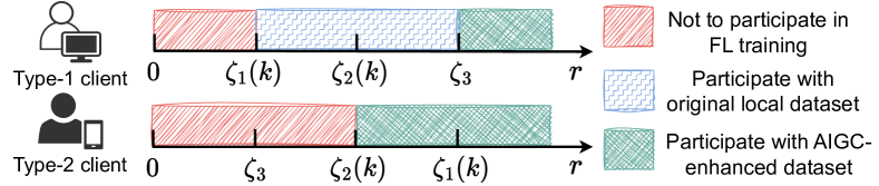
Figure 5: The rational behavior of each client $k$.

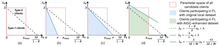
Figure 6: Parameter space of $(s_{k},\lambda_{k})$ for clients.

III-B Server’s Optimal Strategy in Complete Information Scenario

Considering clients’ rational behaviors, the server aims to minimize its cost in (10) by finding the optimal strategy:

$$\mathop{Minimize}\limits_{T,r}\ \mathcal{C}_{cost},$$ (16)

$$\mbox{s.t.}\quad T\in\{1,2,...\},$$ (16a)

$$\quad\quad\,r\in(0,+\infty).$$ (16b)

It is challenging to directly solve problem (16) due to the mutual coupling of the number of global iterations $T$ and the unit data reward benchmark $r$. In what follows, we first derive some useful insights for $r$ under any fixed $T$, based on which, we derive the optimal server’s strategy.

According to clients’ rational behaviors, a uniform unit data reward benchmark $r$ corresponds to a unique participating client set $\mathcal{N}_{r}=\mathcal{N}_{r}^{L}\cup\mathcal{N}_{r}^{A}$. We denote the training error during FL process caused by clients $\mathcal{N}_{r}$ as $\Lambda(\mathcal{N}_{r})=\sum_{k\in\mathcal{N}_{r}^{L}}\nu_{k}(\mathcal{N}_{r})\chi_{k}+\sum_{k\in\mathcal{N}_{r}^{A}}\nu_{k}(\mathcal{N}_{r})\chi_{k,A}$, where $\chi_{k}=(\frac{\psi}{\sqrt{B_{k}}}+\lambda_{k})$ and $\chi_{k,A}=(\frac{\psi}{\sqrt{B_{k}}}+\lambda_{k,A})$. Hence, given a fixed number of global iterations $T$, the server’s cost can be represented as:

$$\mathcal{C}_{server}(T,r)=\!\!\!\!\!\! \!\!\!\!\!\!\gamma_{1}\phi^{hT}\Theta$$ (17)

$$\!\!\!\!\!\!+(1-\phi^{hT})\gamma_{1}\kappa_{1}\Lambda(\mathcal{N}_{r})+\gamma_{2}TR(\mathcal{N}_{r}),$$

where $R(\mathcal{N}_{r})=\sum_{k\in\mathcal{N}_{r}^{L}}d_{k}(1-\frac{\lambda_{k}}{\lambda})+\sum_{k\in\mathcal{N}_{r}^{A}}d_{k}(1-\frac{\lambda_{k,A}}{\lambda})$, which indicates the payment to clients corresponding to unit data reward benchmark $r$ in one global iteration. We next reveal the property of the optimal unit data reward benchmark $r_{o}$:

Proposition 1

In complete information scenario, for any fixed number of iterations $T$, the optimal unit data reward benchmark $r_{o}$ to minimize the server’s cost in (17) must belong to the set of all clients’ indicators $\bm{\zeta}$, i.e.,

$$r_{o}\in\bm{\zeta}=\bigcup_{k\in\mathcal{K}}\{\zeta_{1}(k),\zeta_{2}(k),\zeta_{3}\}.$$ (18)

Proof:

We set $\bm{\zeta}\leftarrow\bm{\zeta}\cup\{\infty\}$ and sort indicators in $\bm{\zeta}$ in ascending order. Assume that $r_{o}\notin\bm{\zeta}$, we can search two neighboring indicators $r_{1}\in\bm{\zeta},r_{2}\in\bm{\zeta}$ such that $r_{1}<r_{o}<r_{2}$. Then, we have $\Lambda(\mathcal{N}_{r_{1}})=\Lambda(\mathcal{N}_{r_{o}})$, since each client’s strategy under reward $r_{1}$ is the same as that under reward $r_{o}$. Furthermore, we have $R(\mathcal{N}_{r_{1}})<R(\mathcal{N}_{r_{o}})$ due to $r_{1}<r_{o}$. As a result, we have $\mathcal{C}_{server}(T,r_{1})<\mathcal{C}_{server}(T,r_{o})$, which contracts with the assumption. Thus, we finish the proof of Proposition 1. ∎

Based on Proposition 1, we next reveal the property of the optimal number of global iterations given a fixed unit data reward benchmark $r$:

Proposition 2

Given a fixed unit data reward benchmark $r$ and the assumption $\Theta>\kappa_{1}\Lambda(\mathcal{N}_{r})$, the server’s cost in (16) is a convex function respect to $T$. By setting the first-order derivative $\frac{\partial\mathcal{C}_{cost}}{\partial T}$ to $0$, the optimal number of global iterations $T^{\ast}(r)$ can be calculated as:

$$T^{\ast}(r)=\log_{\phi^{h}}\left[\frac{\gamma_{2}R(\mathcal{N}_{r})}{\gamma_{1}(-\ln\phi^{h})(\Theta-\kappa_{1}\Lambda(\mathcal{N}_{r}))}\right].$$ (19)

Remark 4: The assumption that $\Theta>\kappa_{1}\Lambda(\mathcal{N}_{r})$ is reasonable since FL model training improves the model performance. We can see that the optimal $T^{\ast}(r)$ is decreasing with the increases of $R(\mathcal{N}_{r})$ and $\Lambda(\mathcal{N}_{r})$, since $\phi^{h}<1$.

Based on above analysis, we can obtain the server’s strategy profile $(T^{\ast}(r),r)$ for each candidate $r$ in $\bm{\zeta}$ set. By calculating the server’ s cost for each strategy profile, we choose the optimal one which has the minimum server’s cost. The above procedure to obtain server’s optimal strategy in complete information scenario is summarized in Algorithm 1. For computational efficiency, Algorithm 1 can obtain the optimal strategy for the server with complexity of $O(2|\mathcal{K}|)$.

Algorithm 1 Server’s optimal strategy in complete information scenario

1:The candidate client set $\mathcal{K}$.

2:Server’s optimal strategy profile $(T_{o},r_{o})$.

3:$\mathcal{S}\leftarrow\emptyset$.

4:for each $r\in\zeta$ do

5:    Calculate $T^{\ast}(r)$ based on (19) and obtain the strategy profile $\mathcal{S}\leftarrow\mathcal{S}\cup\{(T^{\ast}(r),r)\}$.

6:end for

7:Search the optimal strategy profile in $\mathcal{S}$ such that it minimizes server’s cost $\mathcal{C}_{server}$, which is denoted as $(T_{o},r_{o})$.

8:return strategy profile $(T_{o},r_{o})$

IV Incomplete Information Scenario

In incomplete information scenario, the server is only aware of the distributions of data quality $\lambda_{k}$ and the unit data usage cost $s_{k}$, instead of knowing the exact values for client’s attributes $(\lambda_{k},s_{k})$. Hence, we aim to derive the server’s optimal strategy to minimize server’s expected cost.

IV-A Clients’ Behaviors in Incomplete Information Scenario

Without loss of generality, we assume that $\lambda_{k}\in(0,\lambda_{max}]$ and $s_{k}\in(0,s_{max}]$ hold for all clients, where $\lambda_{max}=\lambda$ and $s_{max}<\zeta_{3}=\frac{\lambda\delta}{1-\theta}$ . In incomplete information scenario, the server is aware of the probability density functions of $\lambda_{k}$ and $s_{k}$, which are denoted as $u(\cdot)$ and $v(\cdot)$, respectively. Here, $\lambda_{k}$ and $s_{k}$ are independent with each other.

To intuitively show clients’ behaviors associated with their personal attributes, a two-dimensional parameter space is constructed for all clients based on $s_{k}$ and $\lambda_{k}$. As depicted in Fig. 6(a), all clients fall in the parameter space $D_{space}=\{(s_{k},\lambda_{k})|s_{k}\in(0,s_{max}],\lambda_{k}\in(0,\lambda]\}$ following the joint probability distribution of $s_{k}$ and $\lambda_{k}$. Obviously, type-1 and type-2 clients are divided by the dotted line $\lambda_{k}=-\frac{1-\theta}{\delta}s_{k}+\lambda$. Given the uniform unit data reward benchmark $r$, we can derive the probability of each strategy adopted by a client by considering the following three cases:

• Case (i) ($r\in(0,s_{max})$): According to clients’ rational behaviors (See Theorem 2), each type-1 client $k$ will not participate in FL with AIGC-enhanced dataset (i.e., strategy $\varphi_{k}(1,1)$) due to $r<s_{max}<\zeta_{3}=\frac{\lambda\delta}{1-\theta}$. When $r\geq\zeta_{1}(k)\Rightarrow\lambda_{k}\leq-\frac{\lambda}{r}s_{k}+\lambda$, each type-1 client $k$ will participate in FL with its local dataset. As for each type-2 client $k$, it will not participate in FL since $r<\zeta_{3}<\zeta_{2}(k)$. Accordingly, as illustrated in Fig. 6(b), client whose attribute tuple $(s_{k},\lambda_{k})$ falls within the blue region will participate in FL with its local dataset. Thus, the probability that client $k$ participates in FL can be calculated as $P_{1}=\iint\limits_{D_{1}}u(s_{k})v(\lambda_{k}){\rm d}s_{k}{\rm d}\lambda_{k}$, where $D_{1}=\{(s_{k},\lambda_{k})|s_{k}\in(0,r),\lambda_{k}\in(0,-\frac{\lambda}{r}s_{k}+\lambda)\}$ represents the blue region in Fig. 6(b).

• Case (ii) ($r\in[s_{max},\zeta_{3})$): Similar to the above case, only type-1 clients (i.e., the clients located in the blue region $D_{2}=\{(s_{k},\lambda_{k})|s_{k}\in(0,s_{max}),\lambda_{k}\in(0,-\frac{\lambda}{r}s_{k}+\lambda)\}$ in Fig. 6(c)) will participate in FL with its local dataset. Accordingly, the probability that client $k$ participates in FL can be denoted as $P_{2}=\iint\limits_{D_{2}}u(s_{k})v(\lambda_{k}){\rm d}s_{k}{\rm d}\lambda_{k}.$

• Case (iii) ($r\in[\zeta_{3},\frac{\lambda\delta+s_{max}}{1-\theta}]$): Since $r\geq\zeta_{3}$, all type-1 clients will participate in FL with AIGC-enhanced datasets (i.e., strategy $\varphi_{k}(1,1)$). While each type-2 client $k$ participates in FL with the AIGC-enhanced dataset when $r\geq\zeta_{2}(k)\Rightarrow\lambda_{k}\leq-\frac{\lambda}{\lambda\delta+\theta r}s_{k}+\frac{r\lambda}{\lambda\delta+\theta r}$. Combining two types of clients, we summarize that client whose attribute tuple $(s_{k},\lambda_{k})$ is located in the green region of Fig. 6(d) will participate in FL with AIGC-enhanced datasets. Consequently, the probability that client $k$ participates in FL can be written as $P_{3}=\iint\limits_{D_{3}}u(s_{k})v(\lambda_{k}){\rm d}s_{k}{\rm d}\lambda_{k}$ where $D_{3}=D_{31}\cup D_{32}$, $D_{31}=\{(s_{k},\lambda_{k})|s_{k}\in(0,(1-\theta)r-\lambda\delta),\lambda_{k}\in(0,\lambda)\}$ and $D_{32}=\{(s_{k},\lambda_{k})|s_{k}\in[(1-\theta)r-\lambda\delta,s_{max}),\lambda_{k}\in(0,-\frac{\lambda}{\lambda\delta+\theta r}s_{k}+\frac{r\lambda}{\lambda\delta+\theta r}]\}$.

IV-B The Server’s Expected Cost

Due to the inherent uncertainties in incomplete information scenario, the server endeavors to minimize its expected cost by finding the optimal strategy:

$$\mathop{Minimize}\limits_{T,r}\ \mathbb{E}(\mathcal{C}_{cost}),$$ (20)

$$\mbox{s.t.}\quad T\in\{1,2,...\},$$ (20a)

$$\quad\quad\,r\in(0,+\infty).$$ (20b)

It is challenging to solve problem (20) due to the following two aspects. On the one hand, the calculation for $\mathbb{E}(\mathcal{C}_{cost})$ is non-trivial under a given strategy $(T,r)$ due to the complex clients’ behaviors. On the other hand, the mutual coupling of $T$ and $r$ exacerbates the difficulty to derive the optimal strategy for the server in presence of information asymmetry.

To estimate $\mathbb{E}(\mathcal{C}_{cost})$ under a given strategy $(T,r)$, we first rewrite (20) as follows:

$$\mathbb{E}(\mathcal{C}_{cost})=\gamma_{1}\mathbb{E}(M_{loss})+\gamma_{2}\mathbb{E}(R_{total}),$$ (21)

where

$$\!\!\!\mathbb{E}(M_{loss})=\phi^{hT}\Theta+(1-\phi^{hT})\kappa_{1}\frac{\psi}{\sqrt{h}}\underbrace{\mathbb{E}\left[\sum_{k\in\mathcal{N}_{r}}\frac{\sqrt{d_{k}}}{d(\mathcal{N}_{r})}\right]}_{\bm{M}_{1}}$$

$$\!\!\!+\underbrace{\mathbb{E}\left[\sum_{k\in\mathcal{N}^{L}_{r}}\frac{d_{k}}{d(\mathcal{N}_{r})}\lambda_{k}+\sum_{k\in\mathcal{N}^{A}_{r}}\frac{d_{k}}{d(\mathcal{N}_{r})}\lambda_{k,A}\right]}_{\bm{M}_{2}},$$ (22)

and

$$\mathbb{E}(R_{total})=\gamma_{2}Tr\underbrace{\mathbb{E}(\sum_{k\in\mathcal{N}_{r}}d_{k})}_{\bm{M}_{3}}(1-\frac{\mathbb{E}(\lambda_{k})}{\lambda}).$$ (23)

To calculate (21), we next introduce how to estimate $\bm{M}_{1}$, $\bm{M}_{2}$ and $\bm{M}_{3}$ for cases (i), (ii) and (iii):

IV-B1 Estimation of $\bm{M}_{1}$

The challenge for estimating $\bm{M}_{1}$ is twofold: First, when $d(\mathcal{N}_{r})=\sum_{k\in\mathcal{N}_{r}}d_{k}=0$ (e.g., no client participates in FL), the term $\sum_{k\in\mathcal{N}_{r}}\frac{\sqrt{d_{k}}}{d(\mathcal{N}_{r})}$ is undefined. Second, the value of $d(\mathcal{N}_{r})=\sum_{k\in\mathcal{N}_{r}}d_{k}$ is determined by the set of the recruited client $\mathcal{N}_{r}$.

In light of the first challenge, we utilize a large positive constant $\Omega$ to characterize the cost of gradient error when there is no client participating in FL (i.e., $d(\mathcal{N}_{r})=0$) . Based on this, we construct a random variable $Q$ as follows:

$$Q=\left\{\begin{aligned} &\sum_{k\in\mathcal{N}_{r}}\frac{\sqrt{d_{k}}}{d(\mathcal{N}_{r})},\qquad\mbox{if}\ d(\mathcal{N}_{r})\neq 0,\\ &\Omega,\qquad\mbox{if}\ d(\mathcal{N}_{r})=0.\\ \end{aligned}\right.$$ (24)

By supplementing the definition of $\sum_{k\in\mathcal{N}_{r}}\frac{\sqrt{d_{k}}}{d(\mathcal{N})}$, the value of $\mathbb{E}(Q)$ can be regarded as the estimated value of $\bm{M}_{1}$. Given unit data reward benchmark $r$, directly calculating $\mathbb{E}(Q)$ necessitates an algorithm with complexity of $O(2^{K})$, which inevitably incurs a significant expense.

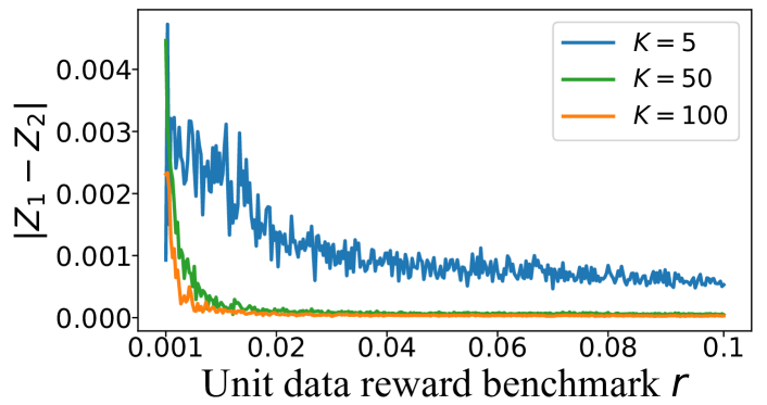
Figure 7: The value of $|Z_{1}-Z_{2}|$ for different unit data reward benchmark $r$.

To calculate $\mathbb{E}(Q)$ with high computational efficiency, we define a random variable $z_{k}\in\{0,1\}$ for each client $k\in\mathcal{K}$ to denote whether to participate in FL given the unit data reward benchmark $r$. Here, we let $z_{k}=1$ with probability $p$ and $z_{k}=0$ with probability $1-p$, where $p$ equals to $P_{1}$, $P_{2}$ and $P_{3}$ for cases (i), (ii) and (iii), respectively. Then, an estimator for random variable $Q$ is constructed by:

$$Z=\frac{\sum_{k\in\mathcal{K}}z_{k}\sqrt{d_{k}}+\epsilon\cdot\prod_{k\in\mathcal{K}}(1-z_{k})}{\sum_{k\in\mathcal{K}}z_{k}d_{k}+\sqrt{\epsilon}\cdot\prod_{k\in\mathcal{K}}(1-z_{k})}+\Omega\cdot\prod_{k\in\mathcal{K}}(1-z_{k}),\!\!\!\!\!\!\!\!\!\!\!\!$$

where $\epsilon\to 0^{+}$. When no client participates in FL (i.e., $\mathcal{N}_{r}=\emptyset$), we have $Z=\sqrt{\epsilon}+\Omega\approx\Omega$. Otherwise, we have $Z=\sum_{k\in\mathcal{N}_{r}}\frac{\sqrt{d_{k}}}{d(\mathcal{N}_{r})}$. Then, we calculate $\mathbb{E}(Z)$ as follows:

$$\mathbb{E}(Z)\!\!\!\!\!\! = \!\!\!\!\!\!\underbrace{\mathbb{E}\left(\frac{\sum_{k\in\mathcal{K}}z_{k}\sqrt{d_{k}}+\epsilon\cdot\prod_{k\in\mathcal{K}}(1-z_{k})}{\sum_{k\in\mathcal{K}}z_{k}d_{k}+\sqrt{\epsilon}\cdot\prod_{k\in\mathcal{K}}(1-z_{k})}\right)}_{Z_{1}}+(1-p)^{K}\Omega\!\!\!$$ (26)

$$\approx \!\!\!\!\!\!\underbrace{\frac{\mathbb{E}(\sum_{k\in\mathcal{K}}z_{k}\sqrt{d_{k}}+\epsilon\cdot\prod_{k\in\mathcal{K}}(1-z_{k}))}{\mathbb{E}(\sum_{k\in\mathcal{K}}z_{k}d_{k}+\sqrt{\epsilon}\cdot\prod_{k\in\mathcal{K}}(1-z_{k}))}}_{Z_{2}}+(1-p)^{K}\Omega$$

$$= \!\!\!\!\!\!\frac{\sum_{k\in\mathcal{K}}p\sqrt{d_{k}}+\epsilon\cdot(1-p)^{K}}{\sum_{k\in\mathcal{K}}pd_{k}+\sqrt{\epsilon}\cdot(1-p)^{K}}+(1-p)^{K}\Omega$$

$$\approx \!\!\!\!\!\!\frac{\sum_{k\in\mathcal{K}}\sqrt{d_{k}}}{\sum_{k\in\mathcal{K}}d_{k}}+(1-p)^{K}\Omega.$$

In the second equation of (26), we use term $Z_{2}$ to approximate term $Z_{1}$ when $\mathcal{N}_{r}\neq\emptyset$. As illustrated in Fig. 7, we show the difference between the real value of $Z_{1}$ and $Z_{2}$ under different values of unit data reward benchmark $r$. For parameter settings, we set $\lambda_{k}\sim Uniform(0,3)$, $s_{k}\sim Uniform(0,0.1)$ and $\epsilon=10^{-8}$. The other parameters’ settings are the same as that in Section V-C. We can see that $|Z_{1}-Z_{2}|$ is small enough with different numbers of candidate clients $K$, indicating that our approximation is reasonable.

By formulating a two-tier nested estimation framework, the quantification of $\mathbb{E}(Q)$ is attained through the estimation of $\mathbb{E}({Z})$, leading to the ultimate derivation of the value of $\bm{M}_{1}$.

IV-B2 Calculation of $\bm{M}_{2}$

As $\bm{M}_{2}$ indicates the expected training gradient error caused by data quality, we have $\sum_{k\in\mathcal{N}^{L}}\frac{d_{k}}{d(\mathcal{N}_{r})}\lambda_{k}+\sum_{k\in\mathcal{N}^{A}}\frac{d_{k}}{d(\mathcal{N}_{r})}\lambda_{k,A}=0$ when $d(\mathcal{N}_{r})=0$ (i.e., $\mathcal{N}_{r}=\emptyset$). Recalling cases (i), (ii) and (iii) discussed in Section IV-A, we have $\mathcal{N}_{r}^{L}=\emptyset$ or $\mathcal{N}_{r}^{A}=\emptyset$ when $\mathcal{N}_{r}=(\mathcal{N}_{r}^{L}\cup\mathcal{N}_{r}^{A})\neq\emptyset$. Hence, we have $\bm{M}_{2}=\mathbb{E}\left[\sum_{k\in\mathcal{N}_{r}}\frac{d_{k}}{d(\mathcal{N}_{r})}\lambda_{k}\right]$ for cases (i) and (ii). In case (iii), we have $\bm{M}_{2}=\mathbb{E}\left[\sum_{k\in\mathcal{N}_{r}}\frac{d_{k}}{d(\mathcal{N})}\lambda_{k,A}\right]$.

For case (i), we can obtain the value of $\bm{M}_{2}$ by calculating the following equation:

$$\mathbb{E}\left[\sum_{k\in\mathcal{N}_{r}}\frac{d_{k}}{d(\mathcal{N}_{r})}\lambda_{k}\right]\!\!=\!\!\mathbb{E}(\lambda_{k})\!\!=\iint\limits_{D_{1}}u(s_{k})v(\lambda_{k})\lambda_{k}{\rm d}s_{k}{\rm d}\lambda_{k}.$$ (27)

Here, the first equation originates from $\sum_{k\in\mathcal{N}_{r}}\frac{d_{k}}{d(\mathcal{N})}=1$ when $\mathcal{N}_{r}\neq 0$. Similarly, we replace the region $D_{1}$ with $D_{2}$ in (27) and obtain the value of $\bm{M}_{2}$ for case (ii). As each recruited clients use AIGC-enhanced datasets for FL model training, the value of $\bm{M}_{2}$ for case (iii) can be calculated by:

$$\!\!\mathbb{E}\!\!\left[\sum_{k\in\mathcal{N}_{r}}\frac{d_{k}}{d(\mathcal{N})}\lambda_{k,A}\right]\!\!=\!\!\mathbb{E}(\lambda_{k,A})=\!\!\iint\limits_{D_{3}}u(s_{k})v(\lambda_{k})\theta\lambda_{k}{\rm d}s_{k}{\rm d}\lambda_{k}.\!\!\!\!\!\!\!\!\!\!\!\!\!\!$$

Here, the second equation originates from $\lambda_{k,A}=\theta\lambda_{k}$.

IV-B3 Calculation of $\bm{M}_{3}$

We have $\bm{M}_{3}=\mathbb{E}(\sum_{k\in\mathcal{K}}z_{k}d_{k})=p(\sum_{k\in\mathcal{K}}d_{k})$.

By substituting $\bm{M}_{1}$, $\bm{M}_{2}$ and $\bm{M}_{3}$ into (21), we can obtain the server’s expected cost given fixed $T$ and $r$.

IV-C Server’s Optimal Strategy in Incomplete Information Scenario

In light of the mutual coupling of $T$ and $r$ in server’s strategy, we first aim to obtain the optimal $r$ by minimizing (20) given a fixed $T$. Due to different clients’ behaviors over different ranges of $r$, problem (20) is naturally decomposed into three subproblems corresponding to cases (i), (ii) and (iii), denoted as $\mathbb{E}[\mathcal{C}_{cost,\it{(i)}}(r)],r\in(0,s_{max})$; $\mathbb{E}[\mathcal{C}_{cost,\it{(ii)}}(r)],r\in[s_{max},\zeta_{3})$ and $\mathbb{E}[\mathcal{C}_{cost,\it{(iii)}}(r)],r\in[\zeta_{3},\frac{\lambda\delta+s_{max}}{1-\theta}]$, respectively. Taking case (i) as an example, the server’s cost under a fixed $T$ can be represented as:

$$\!\!\!\mathbb{E}(\mathcal{C}_{cost,(i)})(r)=\gamma_{1}\phi^{hT}\Theta+\gamma_{1}(1-\phi^{hT})\kappa_{1}\frac{\psi}{\sqrt{h}}\mathbb{E}(Z)$$

$$\!\!\!+\gamma_{1}(1-\phi^{hT})\kappa_{1}\mathbb{E}(\lambda_{k})+\gamma_{2}Tr\mathbb{E}(\sum_{k\in\mathcal{N}_{r}}d_{k})(1-\frac{\mathbb{E}(\lambda_{k})}{\lambda}).$$ (29)

These three subproblems are all single-objective optimization problems in terms of $r$, each involving double integrals with respect to $s_{k}$ and $\lambda_{k}$, and can be easily solved by traditional optimizers. The solution corresponding to the minimum server’s cost among these three subproblems signifies the optimal unit data reward benchmark of $r$ for a given fixed $T$.

Remark 5: A low unit data reward benchmark $r$ may lead to a large $\mathbb{E}(Z)$ in (IV-C), which indicates that the server may suffer from high cost to hedge the risk of no or very few clients participating in FL model training. With a large unit data reward benchmark $r<\zeta_{3}$, there are more clients with low data quality participating in FL, resulting in degraded model performance and high payments. When $r\geq\zeta_{3}$, the server recruits clients to participate in FL with AIGC-enhanced datasets, leading to satisfactory training performance but high payment to clients. Hence, a proper decision of $r$ is significantly important to realize a nice balance between model performance and payment to the clients.

Algorithm 2 Server’s optimal strategy in incomplete information scenario

1:The candidate client set $\mathcal{K}$.

2:Server’s optimal strategy profile $(T_{o},r_{o})$.

3:Obtain $T_{max}$ by solving the problem (30).

4:$\mathcal{S}\leftarrow\emptyset$.

5:for $T=1$ to $T=T_{max}$ do

6:    Calculate the minimum server’s cost among the three subproblems $\mathbb{E}[\mathcal{C}_{cost,\it{(i)}}(r)]$; $\mathbb{E}[\mathcal{C}_{cost,\it{(ii)}}(r)]$ and $\mathbb{E}[\mathcal{C}_{cost,\it{(iii)}}(r)]$ and obtain the corresponding reward as the optimal unit data reward benchmark $r_{T}$.

7:    $\mathcal{S}\leftarrow\mathcal{S}\cup\{(T,r_{T})\}$.

8:end for

9:Search the optimal strategy profile in $\mathcal{S}$ such that minimizes server’s cost, which is denoted as $(T_{o},r_{o})$.

10:return strategy profile $(T_{o},r_{o})$.

We have determined the optimal $r$ for any fixed $T$, which inspires us to globally select the optimal $T$, since $T$ belongs to a limited integer set $[0,T_{max}]$. Next, we introduce how to determine the value of $T_{max}$. Proposition 2 reveals the optimal $T^{\ast}(r)$ given a unit data reward benchmark $r$. Then, the optimal number of global iterations $T_{o}$ must satisfy $T_{o}\leq T_{max}$, where $T_{max}=\max_{r}T^{\ast}(r),\forall r\in(0,\frac{\lambda\delta+s_{max}}{1-\theta}]$. We summarize this conclusion as follows:

Proposition 3

In incomplete information scenario, $T_{max}$ can be determined by solving the following optimization problem $T_{max}=\mathop{Maximize}\limits_{r}\ T^{\ast}$, i.e.,

$$\mathop{Maximize}\limits_{r}\log_{\phi^{h}}\left[\frac{\gamma_{2}\mathbb{E}(R(\mathcal{N}_{r}))}{\gamma_{1}(-\ln\phi^{h})(\Theta-\kappa_{1}\mathbb{E}(\Lambda(\mathcal{N}_{r})))}\right],$$ (30)

$$\qquad\qquad\qquad\mbox{s.t.}\quad r\in(0,\frac{\lambda\delta+s_{max}}{1-\theta}],$$ (30a)

The optimization problem can be decomposed to three subproblems, since $\mathbb{E}(R(\mathcal{N}_{r}))$ and $\mathbb{E}(\Lambda(\mathcal{N}_{r}))$ are different in cases (i), (ii) and (iii). Specifically, we have $\mathbb{E}(R(\mathcal{N}_{r}))=r\mathbb{E}(\sum_{k\in\mathcal{N}_{r}}d_{k})(1-\frac{\mathbb{E}(\lambda_{k})}{\lambda})$ and $\mathbb{E}(\Lambda(\mathcal{N}_{r}))=\gamma_{1}\kappa_{1}\frac{\psi}{\sqrt{h}}\mathbb{E}(Z)+\gamma_{1}\kappa_{1}\mathbb{E}(\lambda_{k})$ for cases (i) and (ii). For case (iii), we have $\mathbb{E}(R(\mathcal{N}_{r}))=r\mathbb{E}(\sum_{k\in\mathcal{N}_{r}}d_{k})(1-\frac{\mathbb{E}(\lambda_{k,A})}{\lambda})$ and $\mathbb{E}(\Lambda(\mathcal{N}_{r}))=\gamma_{1}\kappa_{1}\frac{\psi}{\sqrt{h}}\mathbb{E}(Z)+\gamma_{1}\kappa_{1}\mathbb{E}(\lambda_{k,A})$.

The optimization problem (30) is a single-objective which can be solved by traditional optimizer. Based on the above dicussion, Algorithm 2 summarizes the procedure of obtaining server’s optimal strategy in incomplete information scenario.

V Performance Evaluation

In this section, we conduct experiments to study the impact of different distributions of parameters $s_{k}$ and $\lambda_{k}$ on server’s strategy and cost. Further, we evaluate the performance of our mechanism in incomplete information scenario, compared with complete information scenario. Finally, we compare the training performance of our mechanism with two benchmarks mechanism on real datasets.

V-A Parameter Settings

Experimental environment. We conduct experiments on the device equipped with Ubuntu 18.04.05, CUDA v12.0, GPU (Tesla P100-PCIE) and Intel(R) Xeon(R) CPU (E5-2678 v3).

Datasets and models. To gauge the effectiveness of our incentive mechanism, we consider image classification as the FL training task and conduct extensive evaluations with three widely-used real-world datasets for FL: MNIST [34], CIFAR10 [35] and GTSRB [36]. We employ a multi-layer perception network consisting of a single hidden layer with 256 hidden units as the learning model for MNIST dataset. While we use LeNet [34], which consists of two sets of convolution and pooling layers, then two fully-connected layers with ReLU activation, as the model trained on clients for the complex CIFAR10 dataset. The architecture of model for GTSRB dataset comprises two convolutional layers followed by max-pooling operations, culminating in two fully connected layers.

Data synthesis by AIGC service. Vision models such as diffusion model have demonstrated impressive capability in high-quality image synthesis [16]. In this paper, we leverage a pre-trained diffusion model in [22] to provision the AIGC service for the data synthesis of MNIST, CIFAR10 and GTSRB datasets.

Parameter settings. The values of $\rho$, $\mu$, and $\lambda_{k}$ are dictated by the specific loss function and dataset, which can be estimated within a concise FL training process empirically [37]. For the parameter estimation of MNIST dataset, we set $K=10$ and $\psi=25$. Each client is randomly allocated with $5,000$ data samples under a uniform data distribution over 10 classes. With a learning rate of $\eta=0.01$ and global iteration number of $T=50$, we simulate the FL training process and obtain the estimated value for each parameter: $\rho=37.36$, $\mu=5.48$, and $\beta=0.57$. Similarly, we can obtain $\rho=16.94$, $\mu=2.53$, and $\beta=0.28$ for CIFAR10 dataset by setting $K=10$ and $\psi=10$. Also, we have $\rho=12.49$, $\mu=3.40$, and $\beta=0.78$ for GTSRB dataset by setting $K=43$ and $\psi=10$.

TABLE II: The range of $\lambda_{k}$ with $l$ classes for MNIST dataset.

$l$	$\lambda_{k}$	$l$	$\lambda_{k}$
1	$(0.8,3)$	8	$(0.14,0.18)$
2,3	$(0.42,0.8)$	9	$(0.08,0.14)$
4,5	$(0.32,0.42)$	10	$(0,0.08)$
6,7	$(0.18,0.32)$

TABLE III: The range of $\lambda_{k}$ with $l$ classes for CIFAR10 dataset.

$l$	$\lambda_{k}$	$l$	$\lambda_{k}$
1,2	$(0.76,2)$	6,7	$(0.35,0.46)$
3	$(0.65,0.76)$	8	$(0.23,0.35)$
4	$(0.55,0.65)$	9	$(0.15,0.23)$
5	$(0.46,0.55)$	10	$(0,0.15)$

For $g_{data}$ and $g_{diff}$ on MNIST datasets, we conduct a simple FL training process (e.g., training within 20 global iterations) for both local dataset and generated dataset where all data samples are generated by AIGC service. In order to evaluate the maximum value of the gradient and gradient difference, we simulate the highly non-IID scenario for the two datasets and simultaneously record the maximum gradient norm, and maximum gradient error between local and generated datasets. As a result, we obtain $g_{data}=\max_{t,k}\|\nabla F_{k}(\bm{w}^{t};\mathcal{D}_{MNIST})\|=2.45$ and $g_{diff}=\max_{t,k}\|\nabla F_{k}(\bm{w}^{t};\mathcal{D}_{MNIST})-\nabla F_{k}(\bm{w}^{t};\mathcal{D}_{AIGC})\|=1.05$ for MNIST dataset. Similarly, $g_{data}=1.75$ and $g_{diff}=0.54$ can be acquired for CIFAR10 dataset. In terms of GTSRB datasets, we have $g_{data}=16.51$ and $g_{diff}=12.07$.

As for the non-IID degree $\lambda_{k}$ which is dataset-specified, we estimate the rough range of $\lambda_{k}$ under different data partition cases. Specifically, for the data partition case where client $k$ possesses data samples from $l$ classes, we conduct a simple FL training process with $T=20$ global iterations and record the maximum gradient error between the local gradient of client $k$ and the global gradient, i.e., $\lambda_{k}(l)=\max_{t}\|\nabla F_{k}(\bm{w}^{t})-\nabla F(\bm{w}^{t})\|$. Following this way, we are able to obtain the series values $\lambda_{k}(l),k\in\{1,2,...,10\}$ and calculate the rough range of $\lambda_{k}$ for each data partition cases of MNIST and CIFAR10 datasets, as summarized in Table II and Table III.

V-B Discussion on AIGC-enhanced dataset

In this paper, we employ the AIGC-enhanced dataset, which comprises a mixture of real-world and generated data samples for each client, i.e., retaining some local data samples while introducing generated ones. From a theoretical perspective, we have demonstrated that the data quality of the AIGC-enhanced dataset is superior to that of a dataset consisting of only generated samples (referred to as the AIGC-only dataset) in Section II-B. To further validate our conclusion, we have added experiments to evaluate the training performance of the AIGC-enhanced dataset on the MNIST and CIFAR10 datasets.

In our experiments, we set $K=10$ clients and $T=100$ global iterations for both MNIST and CIFAR10 dataset. Under identical training conditions, we compare training accuracy on original local datset, AIGC-enhanced datasets, and AIGC-only dataset, respectively. For instance, as shown in Fig. 10, we randomly assign $200$ data samples from one class as local dataset for each client. Based on this, we construct AIGC-enhanced dataset (IID dataset) with $10$ classes for each client, comprising a mixture of real-world and generated data samples (discussed in Section II-A in revised paper). For comparison, we generate $200$ data samples with $10$ classes for each client as AIGC-only dataset (IID dataset).

As illustrated in Fig. 10, Fig. 10, and Fig. 10, the AIGC-enhanced dataset consistently achieves the highest accuracy across various settings. The poor performance of adoption AIGC-only dataset is attributed to the distribution differences between generated data samples (e.g., $\bm{p}_{a}$) and real-world data samples (e.g., $\bm{p}$). On the MNIST dataset, when clients possess a small number of classes, the proportion of generated data samples is higher in the AIGC-enhanced dataset, resulting in similar performance compared with the AIGC-only dataset. Similarly, superior training accuracy of the AIGC-enhanced dataset on CIFAR10 datasets is evident in Fig. 13, Fig. 13, and Fig. 13. Notably, the AIGC-enhanced dataset not only demonstrates excellent training accuracy but also significantly reduces the costs associated with the data generation process compared to the AIGC-only dataset. The results obtained from the MNIST and CIFAR10 datasets corroborate our theoretical findings and highlight the advantages of utilizing the AIGC-enhanced dataset.

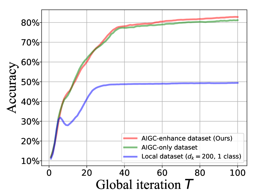
Figure 8: Accuracy of each generated datasets when local dataset with $d_{k}=200$ and $1$ class on MNIST dataset.

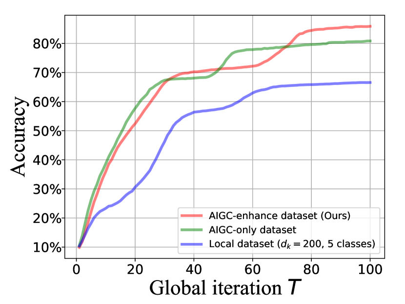
Figure 9: Accuracy of each generated datasets when local dataset with $d_{k}=200$ and $5$ classes on MNIST dataset.

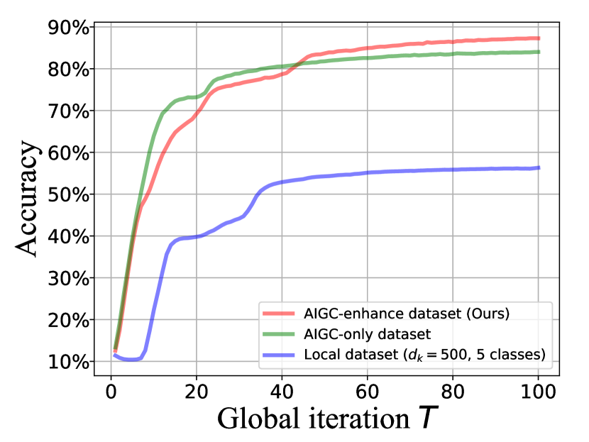
Figure 10: Accuracy of each generated datasets when local dataset with $d_{k}=500$ and $5$ classes on MNIST dataset.

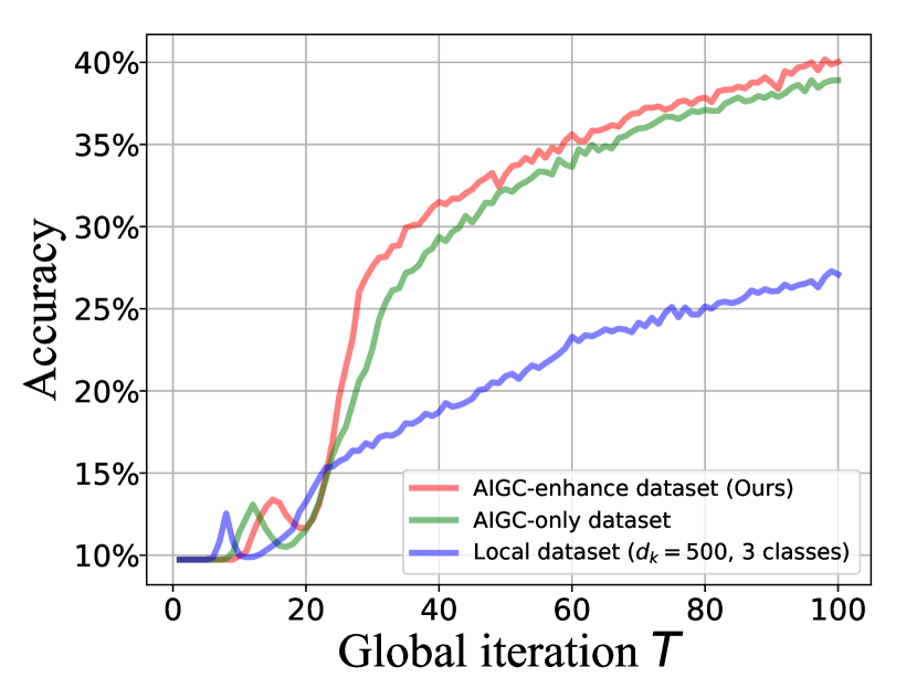
Figure 11: Accuracy of each generated dataset when local dataset with $d_{k}=500$ and $3$ classes on CIFAR10 dataset.

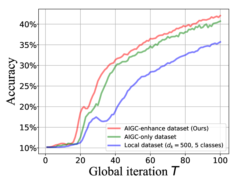
Figure 12: Accuracy of each generated dataset when local dataset with $d_{k}=500$ and $5$ classes on CIFAR10 dataset.

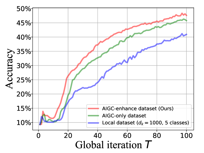
Figure 13: Accuracy of each generated dataset when local dataset with $d_{k}=1000$ and $5$ classes on CIFAR10 dataset.

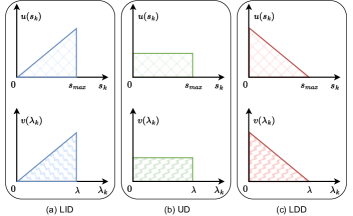
Figure 14: An illustration of three different kinds of distributions for $s_{k}$ and $\lambda_{k}$.

V-C Impact of Distributions of $s_{k}$ and $\lambda_{k}$ on Server’s Strategy

For the ease of investigating the impact of the distribution of client’s attributes (e.g., $s_{k}$ and $\lambda_{k}$) on server’s strategy, we consider the following three simple distributions for $s_{k}\in(0,s_{max}]$ and $\lambda_{k}\in(0,\lambda)$:

• Linear increasing distribution (LID): probability density functions of $s_{k}$ and $\lambda_{k}$ are set to $u(s_{k})=\frac{2}{s_{max}^{2}}s_{k}$ and $v(\lambda_{k})=\frac{2}{\lambda^{2}}\lambda_{k}$, respectively.

• Uniform distribution (UD): $u(s_{k})=\frac{1}{s_{max}}$ and $v(\lambda_{k})=\frac{1}{\lambda}$ are adopted for $s_{k}$ and $\lambda_{k}$, respectively.

• Linear decreasing distribution (LDD): probability density functions of $u(s_{k})=-\frac{2}{s_{max}^{2}}s_{k}+\frac{2}{s_{max}}$ and $v(\lambda_{k})=-\frac{2}{\lambda^{2}}\lambda_{k}+\frac{2}{\lambda}$ are utilized for $s_{k}$ and $\lambda_{k}$, respectively.

Fig. 14 gives an intuitive illustration of the three different kinds of distributions. In the experiments, we set $\lambda=3$ and $s_{max}=0.1$ based on the parameter evaluation results on MNIST dataset. For the parameter setting of the server, we set $\gamma_{1}=10^{5}$ and $\gamma_{2}=1$. The payment of using one generated data sample which is obtained by leveraging AIGC service is set as $s_{AI}=0.5$. For ease of comparison, datasize for each client $k$ is set to be $d_{k}\in(100,300)$ for all the three cases with different distributions of $s_{k}$ and $\lambda_{k}$.

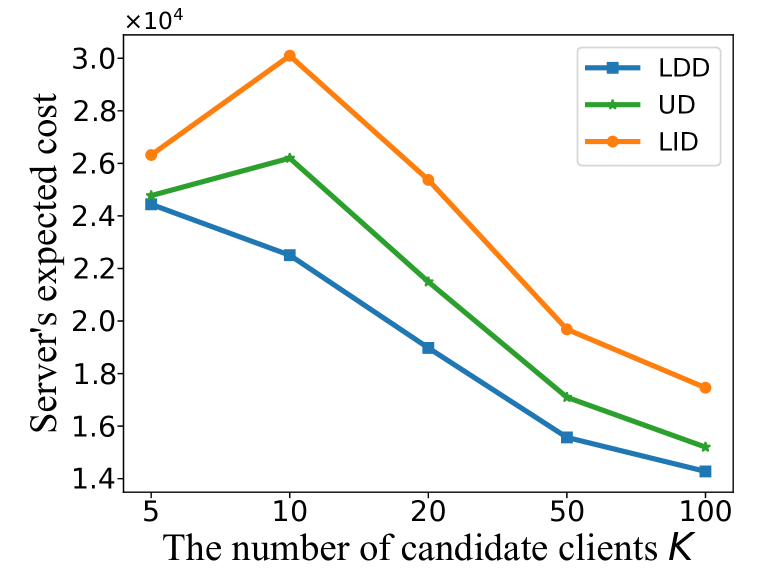
Figure 15: The server’s expected cost for each distribution under different number of candidate clients $K$.

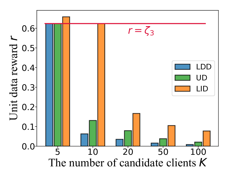
Figure 16: The unit data reward benchmark for each distribution under different number of candidate clients $K$.

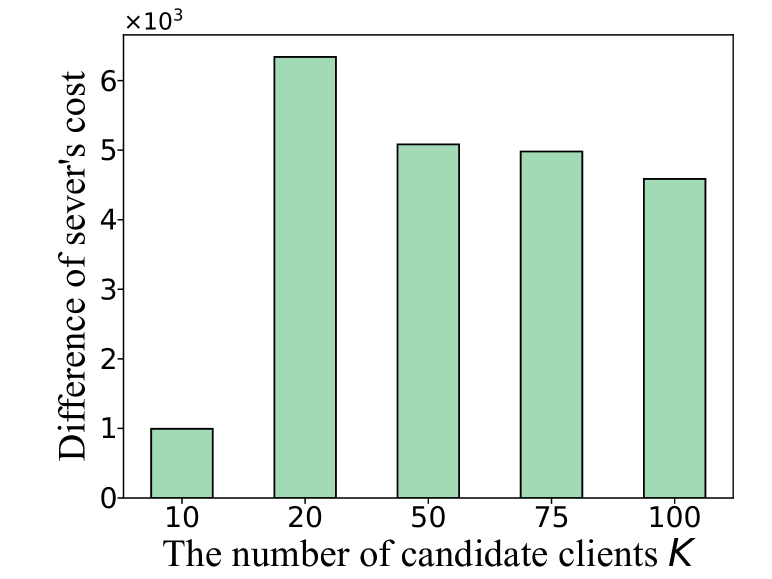
Figure 17: The difference of server’s cost between complete and incomplete information scenarios.

We conduct experiments under three kinds of distributions of $s_{k}$ and $\lambda_{k}$ with different numbers of $K$, and show the changes of server’s cost and unit data reward benchmark $r$. To reduce the error caused by randomness, we repeat the calculation process under each distribution case $10$ times and compute the average of the results. As depicted in Fig. 17 and Fig. 17, our incentive mechanism achieves the lowest server’s expected cost in LDD, since the server in LDD scenario can easily recruit high-quality clients with lower payment cost and hence tends to publish a lower $r$ than UD and LID scenarios. In contrast, the server has to publish the highest uniform unit data reward benchmark $r$ in LID scenario for fear of the case that there are no clients recruited in FL due to a low unit data reward benchmark. With the increase of the number of candidate clients $K$, the number of high-quality clients in the candidate client set increase accordingly. Due to the lower risk of not having enough high-quality clients available for recruitment, the server tends to publish a lower $r$. Besides, the difference of the server’s expected costs among the three distributions decrease with the increase of the number of candidate clients when $K\geq 10$.

Interestingly, as shown in Fig. 17, the sever adopts $r\geq\zeta_{3}$ as the unit data reward benchmark when $K=5$. The reason is twofold: 1) with a small number of candidate clients, the server faces the risk of not recruiting enough clients for FL model training if an adequately high reward is not offered; 2) since the number of candidate clients is small, the server is inclined to incentivize clients to participate in FL with their AIGC-enhanced datasets. This implies that introducing generated data in FL possesses the capacity to significantly reduce server expenses, especially in scenarios characterized by limited candidate clients with lower data quality.

TABLE IV: The average unit data reward benchmark $r$ for different information scenarios.

	$K=10$	$K=20$	$K=50$	$K=75$	$K=100$
Complete	$0.3910$	$0.2705$	$0.0209$	$0.0154$	$0.0272$
Incomplete	$\bm{0.6238}$	$0.0812$	$0.0395$	$0.0280$	$0.0218$

V-D Difference of Server’s Cost between Complete and Incomplete Information Scenarios

To study the difference of server’s cost under complete and incomplete information scenarios, the datasize of each client is set to be $d_{k}=30$ to remove the impact of client’s datasize. For each client $k$, we set $s_{k}\sim Uniform(0,0.1)$ and $\lambda_{k}\sim Uniform(0,3)$ based on the parameter estimation results of MNIST dataset. For the parameter setting of the server, we set $\gamma_{1}=0.8\cdot 10^{5}$ and $\gamma_{2}=1$. The payment of using one data sample generated by AIGC service is set as $s_{AI}=0.8$.

Fig. 17 and Table IV show the difference of server’s cost between complete and incomplete information scenario and the corresponding averaged unit data reward benchmark $r$ for the two cases. To reduce the error caused by randomness, we conduct experiments $10$ times and average the results for the two cases. As depicted in Fig. 17, when $K\geq 20$, the difference of server’s costs between complete and incomplete information scenarios decreases with the increase of the number of candidate clients $K$. When $K=10$, the difference of server’s costs between the two information scenarios is the lowest, since the server recruits clients with AIGC-enhanced datasets by setting $r=\zeta_{3}=0.6238$ in incomplete information scenario. In essence, in instances where the amount of candidate clients is limited, the introduction of AIGC-enhanced datasets serves to alleviate server’s costs stemming from information asymmetry. However, as the quantity of candidate clients escalates, there’s a rise in the presence of high-quality clients (exhibiting lower $\lambda_{k}$ and lower $s_{k}$). Consequently, the server’s reliance on generated data diminishes. Conversely, offering a uniformly increased $r$ to a larger number of clients which use AIGC-enhanced datasets will result in heightened payments to clients.

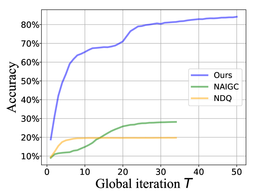
Figure 18: The accuracy of each mechanism on MNIST dataset.

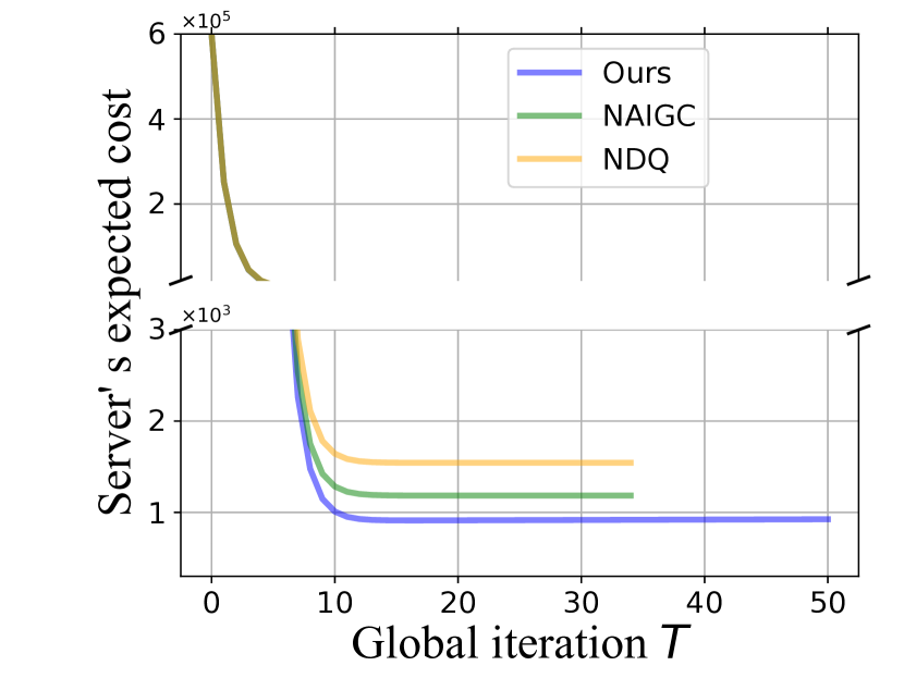
Figure 19: The server’s expected cost of each mechanism on MNIST dataset.

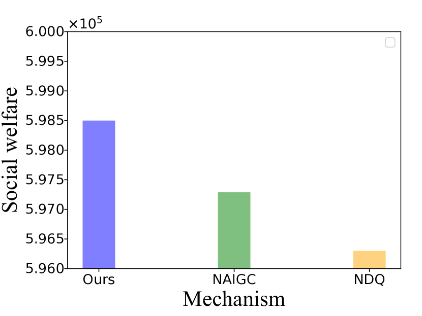
Figure 20: The social welfare of each mechanism on MNIST dataset.

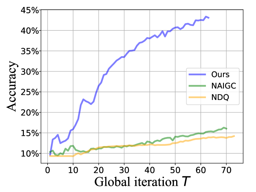
Figure 21: The accuracy of each mechanism on CIFAR10 dataset.

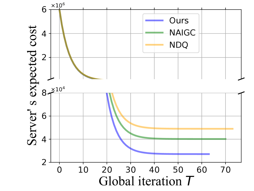
Figure 22: The server’s expected cost of each mechanism on CIFAR10 dataset.

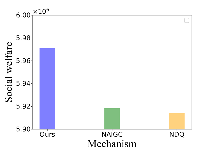
Figure 23: The social welfare of each mechanism on CIFAR10 dataset.

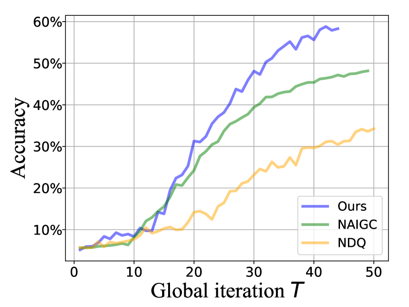
Figure 24: The accuracy of each mechanism on GTSRB dataset.

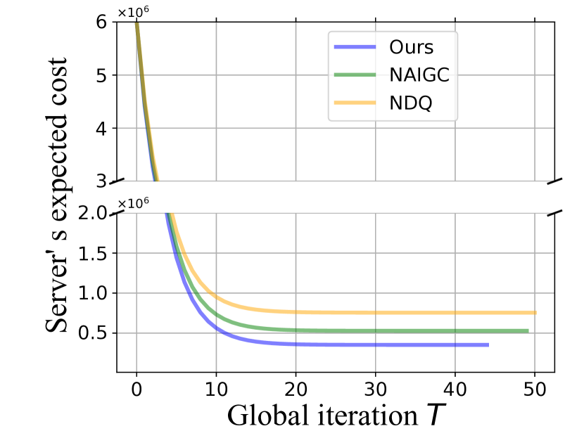
Figure 25: The server’s expected cost of each mechanism on GTSRB dataset.

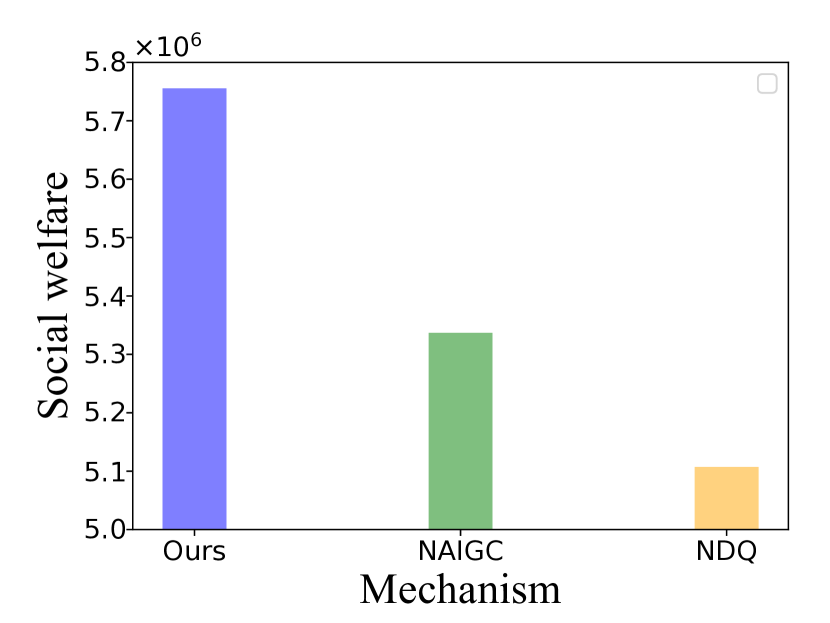
Figure 26: The social welfare of each mechanism on GTSRB dataset.

V-E Training Performance Comparison

We compare the training performance of our proposed mechanism with the following two benchmarks:

• No AIGC (NAIGC): The server considers data quality of clients while neglecting that clients may choose to obtain a high-quality dataset by using AIGC service.

• No data quality (NDQ): The server neglects the data quality of the clients and assigns payment $rd_{k}$ to each client $k$.

We consider FL scenarios with $K=30$ clients on MNIST, CIFAR10 and GTSRB datasets. For the experiments on MNIST dataset, the server’s parameters are set as $\gamma_{1}=10^{5}$ and $\gamma_{2}=0.01$. We set $\lambda_{k}\sim uniform(0,3)$ and $s_{k}\sim uniform(0,10^{-3})$ for each client $k$. Based on the value of $\lambda_{k}$, we can find the number of classes $l$ for the data samples of client $k$ from Table II, and hence assign $d_{k}\in[100,300]$ data samples from $l$ classes randomly for each client $k$. As for CIFAR10 dataset, we set $\gamma_{1}=10^{6}$ and $\gamma_{2}=0.01$ for the server, and set $\lambda_{k}\sim uniform(0,2)$ and $s_{k}\sim uniform(0,5\cdot 10^{-3})$ for each client $k$. According to Table III, we can find the number of classes $l$ for the data samples of client $k$, and then assign $d_{k}\in[300,500]$ data samples from $l$ classes randomly for each client $k$ based on the value of $\lambda_{k}$. As for GTSRB dataset, we set $\gamma_{1}=10^{6}$ and $\gamma_{2}=0.01$ for the server, and set $\lambda_{k}\sim uniform(0,10)$ and $s_{k}\sim uniform(0,5\cdot 10^{-3})$ for each client $k$. In light of data samples with large number of classes (e.g., $43$ classes) on GTSRB dataset, to simulate the uniform distribution of $\lambda_{k}$, we assign $d_{k}\in[1000,2000]$ data samples with a random number of classes $l\in[4,43]$ for each client $k$. The unit cost or payment for one generated data sample is set to $s_{AI}=0.01$ for MNIST, CIFAR10 and GTSRB dataset.

To show the performance of our proposed mechanism, we evaluate the server’s expected cost, training accuracy and social welfare on MNIST, CIFAR10 and GTSRB dataset, respectively. Here, the social welfare is defined as the sum of server’s cost reduction and the total utilities of all clients. As shown in Fig. 20 and Fig. 20, our mechanism achieves the highest accuracy (i.e., $84.15\%$) and the lowest server’s cost compared with NAIGC and NDQ methods on MNIST dataset. This is because that NAIGC only considers the data quality of the local data for the clients, without introducing the generated data for data quality improvement, thus resulting in a degraded model accuracy. Also, as NDQ selects clients based on data quantity while neglecting the heterogeneity of data quality among clients, NDQ is inclined to select clients with lower data quality and hence achieves the lowest training accuracy. By introducing data generation capability and data quality awareness in our mechanism, clients can utilize data generation technique to enhance data quality, enabling FL model to converge to superior performance compared to NAIGC and NDQ, while also achieving the highest social welfare.

Similarly, our mechanism surpasses NDQ and NAIGC on the CIFAR10 dataset, achieving the highest training accuracy and social welfare while reducing server costs by 44.61% and 32.45%, respectively, as shown in Fig. 23, Fig. 23, and Fig. 23. In presence of dataset with more classes, such as GTSRB dataset, our mechanism still exhibits superior performance in terms of training accuracy and social welfare and expected server’s cost, as illustrated in Fig. 26, Fig. 26 and Fig.26. Notably, our proposed mechanism achieves cost reductions of 53.34% and 33.29% compared to NDQ and NAIGC, respectively. These results underscore the robustness of our proposed mechanism across diverse datasets.

VI Related Work

A plethora of studies on federated learning concentrate on improving training efficiency and final model performance [38, 39]. For instance, Jeong et al. devise federated augmentations approach to rectify non-IID dataset for performance improvement [15]. By leveraging AIGC service, clients in FL can conduct data synthesis to mitigate data heterogeneity issue [17]. However, most of the results are derived under an optimistic assumption that clients participate in FL voluntarily, and adopt AIGC services to generate data unconditionally, which may be unrealistic without proper incentives.

Considering the data-computing cost and data generation cost (incurred by adopting AIGC service) of clients, incentive mechanism design is necessary for the server to compensate the cost of clients reasonably. However, existing works on incentive mechanism design for FL exhibit the following limitations. First, most of them considers only one or two dimensions of clients’ information (e.g., data-computing cost, data amount, etc.) for contribution evaluation [40, 32, 41], which may not be directly applicable in realistic FL scenarios with data and resource heterogeneity. Second, few studies consider to capture the relationship between the quality of local model updates (which is related to local data distribution) and the global learning performance [42, 43, 44]. Third, most existing incentive mechanisms assume that the server is aware of all clients’ attributes, which is unrealistic in practice [45], [46]. Fourth, faced the temptation of being rewarded, rational clients may optionally generate a high-quality data to participate in FL with a higher reward [17], which further complicates the incentive mechanism design due to the complex client behaviors and is less understood in existing studies.

There exist some emerging works attempt to deal with the aforementioned issues in different manners. For example, the authors study incentive mechanism with multi-dimensional clients’ private information under different levels of information asymmetry by contract theory [24, 33, 44]. The author propose a multi-dimensional procurement auction for incentive mechanism in FL based on auction analysis framework. Along a different line, in this paper we propose a lightweight data quality-aware incentive mechanism for AIGC-empowered FL.

VII Conclusion

In this paper, we propose a data quality-aware incentive mechanism to encourage clients’ participation in AIGC-empowered FL scenario. With rigorous analysis of convergence performance of FL model trained using a blend of real-world and generated data samples, we derive the optimal server’s incentive strategies both in complete and incomplete information scenarios. Extensive experimental results demonstrate that introducing AIGC service for FL scenarios enables significant cost reduction for the server.

References

- [1] Dinh C Nguyen, Ming Ding, Pubudu N Pathirana, Aruna Seneviratne, Jun Li, Dusit Niyato, Octavia Dobre, and H Vincent Poor. 6g internet of things: A comprehensive survey. IEEE Internet of Things Journal, 9(1):359–383, 2021.
- [2] Zhi Zhou, Xu Chen, En Li, Liekang Zeng, Ke Luo, and Junshan Zhang. Edge intelligence: Paving the last mile of artificial intelligence with edge computing. Proceedings of the IEEE, 107(8):1738–1762, 2019.
- [3] Paul Voigt and Axel Von dem Bussche. The eu general data protection regulation (gdpr). A Practical Guide, 1st Ed., Cham: Springer International Publishing, 2017.
- [4] Brendan McMahan, Eider Moore, Daniel Ramage, Seth Hampson, and Blaise Aguera y Arcas. Communication-efficient learning of deep networks from decentralized data. In Artificial Intelligence and Statistics, pages 1273–1282. PMLR, 2017.
- [5] Muhammad Shayan, Clement Fung, Chris JM Yoon, and Ivan Beschastnikh. Biscotti: A ledger for private and secure peer-to-peer machine learning. arXiv preprint arXiv:1811.09904, 2018.
- [6] Han Yu, Zelei Liu, Yang Liu, Tianjian Chen, Mingshu Cong, Xi Weng, Dusit Niyato, and Qiang Yang. A fairness-aware incentive scheme for federated learning. In Proceedings of the AAAI/ACM Conference on AI, Ethics, and Society, pages 393–399, 2020.
- [7] Tra Huong Thi Le, Nguyen H. Tran, Yan Kyaw Tun, Minh N. H. Nguyen, Shashi Raj Pandey, Zhu Han, and Choong Seon Hong. An incentive mechanism for federated learning in wireless cellular networks: An auction approach. IEEE Transactions on Wireless Communications, 20(8):4874–4887, 2021.
- [8] Miao Hu, Wenzhuo Yang, Zhenxiao Luo, Xuezheng Liu, Yipeng Zhou, Xu Chen, and Di Wu. Autofl: A bayesian game approach for autonomous client participation in federated edge learning. IEEE Transactions on Mobile Computing, 23(1):194–208, 2024.
- [9] Jinlong Pang, Jieling Yu, Ruiting Zhou, and John CS Lui. An incentive auction for heterogeneous client selection in federated learning. IEEE Transactions on Mobile Computing, 2022.
- [10] Qinbin Li, Yiqun Diao, Quan Chen, and Bingsheng He. Federated learning on non-iid data silos: An experimental study. In 2022 IEEE 38th International Conference on Data Engineering (ICDE), pages 965–978. IEEE, 2022.
- [11] Yifang Ma, Zhenyu Wang, Hong Yang, and Lin Yang. Artificial intelligence applications in the development of autonomous vehicles: A survey. IEEE/CAA Journal of Automatica Sinica, 7(2):315–329, 2020.
- [12] Zhihang Song, Zimin He, Xingyu Li, Qiming Ma, Ruibo Ming, Zhiqi Mao, Huaxin Pei, Lihui Peng, Jianming Hu, Danya Yao, and Yi Zhang. Synthetic datasets for autonomous driving: A survey. IEEE Transactions on Intelligent Vehicles, 9(1):1847–1864, 2024.
- [13] Tongnian Wang, Yan Du, Yanmin Gong, Kim-Kwang Raymond Choo, and Yuanxiong Guo. Applications of federated learning in mobile health: scoping review. Journal of Medical Internet Research, 25:e43006, 2023.
- [14] Hongyang Du, Zonghang Li, Dusit Niyato, Jiawen Kang, Zehui Xiong, Dong In Kim, et al. Enabling ai-generated content (aigc) services in wireless edge networks. arXiv preprint arXiv:2301.03220, 2023.
- [15] Eunjeong Jeong, Seungeun Oh, Hyesung Kim, Jihong Park, Mehdi Bennis, and Seong-Lyun Kim. Communication-efficient on-device machine learning: Federated distillation and augmentation under non-iid private data. arXiv preprint arXiv:1811.11479, 2018.
- [16] Jonathan Ho and Tim Salimans. Classifier-free diffusion guidance. arXiv preprint arXiv:2207.12598, 2022.
- [17] Peichun Li, Hanwen Zhang, Yuan Wu, Liping Qian, Rong Yu, Dusit Niyato, and Xuemin Shen. Filling the missing: Exploring generative ai for enhanced federated learning over heterogeneous mobile edge devices. IEEE Transactions on Mobile Computing, 2024.
- [18] Zijian Li, Yuchang Sun, Jiawei Shao, Yuyi Mao, Jessie Hui Wang, and Jun Zhang. Feature matching data synthesis for non-iid federated learning. IEEE Transactions on Mobile Computing, pages 1–16, 2024.
- [19] Jiangtian Nie, Jun Luo, Zehui Xiong, Dusit Niyato, and Ping Wang. A stackelberg game approach toward socially-aware incentive mechanisms for mobile crowdsensing. IEEE Transactions on Wireless Communications, 18(1):724–738, 2018.
- [20] Shehan Edirimannage, Charitha Elvitigala, Ibrahim Khalil, Primal Wijesekera, and Xun Yi. Qarma-fl: Quality-aware robust model aggregation for mobile crowdsourcing. IEEE Internet of Things Journal, 2023.
- [21] Zhao Yue, Li Meng, Lai Liangzhen, Suda Naveen, Civin Damon, and Chandra Vikas. Federated learning with non-iid data. arXiv preprint arXiv:1806.00582, 2018.
- [22] Jonathan Ho, Ajay Jain, and Pieter Abbeel. Denoising diffusion probabilistic models. Advances in neural information processing systems, 33:6840–6851, 2020.
- [23] Lucas Bourtoule, Varun Chandrasekaran, Christopher A Choquette-Choo, Hengrui Jia, Adelin Travers, Baiwu Zhang, David Lie, and Nicolas Papernot. Machine unlearning. In 2021 IEEE Symposium on Security and Privacy (SP), pages 141–159. IEEE, 2021.
- [24] Ningning Ding, Zhixuan Fang, and Jianwei Huang. Optimal contract design for efficient federated learning with multi-dimensional private information. IEEE Journal on Selected Areas in Communications, 39(1):186–200, 2020.
- [25] Nguyen H Tran, Wei Bao, Albert Zomaya, Minh NH Nguyen, and Choong Seon Hong. Federated learning over wireless networks: Optimization model design and analysis. In IEEE INFOCOM 2019-IEEE conference on computer communications, pages 1387–1395. IEEE, 2019.
- [26] Kang Wei, Jun Li, Ming Ding, Chuan Ma, Howard H. Yang, Farhad Farokhi, Shi Jin, Tony Q. S. Quek, and H. Vincent Poor. Federated learning with differential privacy: Algorithms and performance analysis. IEEE Transactions on Information Forensics and Security, 15:3454–3469, 2020.
- [27] Amirsina Torfi, Rouzbeh A Shirvani, Yaser Keneshloo, Nader Tavaf, and Edward A Fox. Natural language processing advancements by deep learning: A survey. arXiv preprint arXiv:2003.01200, 2020.
- [28] Cicero Dos Santos and Maira Gatti. Deep convolutional neural networks for sentiment analysis of short texts. In Proceedings of COLING 2014, the 25th international conference on computational linguistics: technical papers, pages 69–78, 2014.
- [29] Rie Johnson and Tong Zhang. Semi-supervised convolutional neural networks for text categorization via region embedding. Advances in neural information processing systems, 28, 2015.
- [30] Nima Mohammadi, Jianan Bai, Qiang Fan, Yifei Song, Yang Yi, and Lingjia Liu. Differential privacy meets federated learning under communication constraints. IEEE Internet of Things Journal, 9(22):22204–22219, 2021.
- [31] Ofer Dekel, Ran Gilad-Bachrach, Ohad Shamir, and Lin Xiao. Optimal distributed online prediction using mini-batches. Journal of Machine Learning Research, 13(1), 2012.
- [32] Lefeng Zhang, Tianqing Zhu, Ping Xiong, Wanlei Zhou, and S Yu Philip. A robust game-theoretical federated learning framework with joint differential privacy. IEEE Transactions on Knowledge and Data Engineering, 35(4):3333–3346, 2022.
- [33] Ningning Ding, Zhixuan Fang, and Jianwei Huang. Incentive mechanism design for federated learning with multi-dimensional private information. In 2020 18th International Symposium on Modeling and Optimization in Mobile, Ad Hoc, and Wireless Networks (WiOPT), pages 1–8. IEEE, 2020.
- [34] Yann LeCun, Léon Bottou, Yoshua Bengio, and Patrick Haffner. Gradient-based learning applied to document recognition. Proceedings of the IEEE, 86(11):2278–2324, 1998.
- [35] Alex Krizhevsky, Geoffrey Hinton, et al. Learning multiple layers of features from tiny images. 2009.
- [36] Sebastian Houben, Johannes Stallkamp, Jan Salmen, Marc Schlipsing, and Christian Igel. Detection of traffic signs in real-world images: The german traffic sign detection benchmark. In The 2013 International Joint Conference on Neural Networks (IJCNN), pages 1–8, 2013.
- [37] Shiqiang Wang, Tiffany Tuor, Theodoros Salonidis, Kin K. Leung, Christian Makaya, Ting He, and Kevin Chan. Adaptive federated learning in resource constrained edge computing systems. IEEE Journal on Selected Areas in Communications, 37(6):1205–1221, 2019.
- [38] Peter Kairouz, H Brendan McMahan, Brendan Avent, Aurélien Bellet, Mehdi Bennis, Arjun Nitin Bhagoji, Kallista Bonawitz, Zachary Charles, Graham Cormode, Rachel Cummings, et al. Advances and open problems in federated learning. Foundations and Trends® in Machine Learning, 14(1–2):1–210, 2021.
- [39] Jin-woo Lee, Jaehoon Oh, Yooju Shin, Jae-Gil Lee, and Se-Young Yoon. Accurate and fast federated learning via iid and communication-aware grouping. arXiv preprint arXiv:2012.04857, 2020.
- [40] Tra Huong Thi Le, Nguyen H Tran, Yan Kyaw Tun, Minh NH Nguyen, Shashi Raj Pandey, Zhu Han, and Choong Seon Hong. An incentive mechanism for federated learning in wireless cellular networks: An auction approach. IEEE Transactions on Wireless Communications, 20(8):4874–4887, 2021.
- [41] Zhilin Wang, Qin Hu, Ruinian Li, Minghui Xu, and Zehui Xiong. Incentive mechanism design for joint resource allocation in blockchain-based federated learning. IEEE Transactions on Parallel and Distributed Systems, 34(5):1536–1547, 2023.
- [42] Shashi Raj Pandey, Nguyen H Tran, Mehdi Bennis, Yan Kyaw Tun, Aunas Manzoor, and Choong Seon Hong. A crowdsourcing framework for on-device federated learning. IEEE Transactions on Wireless Communications, 19(5):3241–3256, 2020.
- [43] Yufeng Zhan, Peng Li, Zhihao Qu, Deze Zeng, and Song Guo. A learning-based incentive mechanism for federated learning. IEEE Internet of Things Journal, 7(7):6360–6368, 2020.
- [44] Rongfei Zeng, Shixun Zhang, Jiaqi Wang, and Xiaowen Chu. Fmore: An incentive scheme of multi-dimensional auction for federated learning in mec. In 2020 IEEE 40th international conference on distributed computing systems (ICDCS), pages 278–288. IEEE, 2020.
- [45] S. R. Pandey, N. H. Tran, M. Bennis, Y. K. Tun, Z. Han, and C. S. Hong. Incentivize to build: A crowdsourcing framework for federated learning. In 2019 IEEE Global Communications Conference (GLOBECOM), pages 1–6, Dec. 2019.
- [46] Tra Huong Thi Le, Nguyen H. Tran, Yan Kyaw Tun, Minh N. H. Nguyen, Shashi Raj Pandey, Zhu Han, and Choong Seon Hong. An incentive mechanism for federated learning in wireless cellular network: An auction approach. IEEE Transactions on Wireless Communications, pages 1–1, 2021.