A Mathematical Certification for Positivity Conditions in Neural Networks with Applications to Partial Monotonicity and Ethical AI

Abstract

Artificial Neural Networks (ANNs) have become a powerful tool for modeling complex relationships in large-scale datasets. However, their black-box nature poses ethical challenges. In certain situations, ensuring ethical predictions might require following specific partial monotonic constraints. However, certifying if an already-trained ANN is partially monotonic is challenging. Therefore, ANNs are often disregarded in some critical applications, such as credit scoring, where partial monotonicity is required. To address this challenge, this paper presents a novel algorithm (LipVor) that certifies if a black-box model, such as an ANN, is positive based on a finite number of evaluations. Therefore, as partial monotonicity can be stated as a positivity condition of the partial derivatives, the LipVor Algorithm can certify whether an already trained ANN is partially monotonic. To do so, for every positively evaluated point, the Lipschitzianity of the black-box model is used to construct a specific neighborhood where the function remains positive. Next, based on the Voronoi diagram of the evaluated points, a sufficient condition is stated to certify if the function is positive in the domain. Compared to prior methods, our approach is able to mathematically certify if an ANN is partially monotonic without needing constrained ANN’s architectures or piece-wise linear activation functions. Therefore, LipVor could open up the possibility of using unconstrained ANN in some critical fields. Moreover, some other properties of an ANN, such as convexity, can be posed as positivity conditions, and therefore, LipVor could also be applied.

I Introduction

Artificial Neural networks (ANNs) have gained significant attention as a powerful tool for modeling complex non-linear relationships and state-of-the-art performance in many real-world applications [1], [2]. Therefore, ANNs have been an extraordinarily active and promising research field in recent decades. Its development is justified by the encouraging results obtained in many fields including speech recognition [3], computer vision [4], financial applications [5] and many others [6],[7].

However, ANNs are considered black-box models as their analytical expression is hardly interpretable, and therefore, they can only be analyzed in terms of the inputs and outputs. Thus, ANNs can pose a significant challenge in fields where interpretability and transparency are often critical considerations [8], [9]. This needs for explainability has caused the field of explainable artificial intelligence (xAI) to grow substantially in recent years [10]. Consequently, there have been many approaches trying to explain how neural networks are computing their prediction [11], [12], [13].

Nevertheless, explainability alone is insufficient when applying models to critical services such as medicine [9] or credit scoring [14]. As the number of available variables for the model’s training grows, ANN risks capturing spurious or irrelevant patterns in the data. Therefore, the ability to interpret the estimations is inadequate if an ANN generates unfair predictions [15]. Consequently, training ANNs for critical applications should not only focus on explainability, but it must be guaranteed that the model generates controlled predictions to ensure robustness (i.e., the ability to maintain performance despite variations or perturbations in input data) and ethical fairness (i.e., the model adherence to moral principles).

One approach for ensuring that the model behaves appropriately is to incorporate prior knowledge from the human expert into the model. One example where leveraging prior expertise can enhance the model’s robustness occurs when dealing with partial monotonic constraints. By applying a partial monotonic constraint, the model’s output function is forced to be partially monotonic. Therefore, if an increasing (resp. decreasing) partial monotonic constraint is imposed, then the model predictions should increase (resp. decrease) whenever a set of input values increases. By employing these constraints, partial monotonicity can improve the model’s interpretability, particularly for deep neural networks [16].

Moreover, in some cases, partial monotonicity is not just a matter of enhancing explainability and robustness but is often a requisite [17]. For instance, in loan approval, it is coherent that an applicant with a better credit history has more possibilities of getting a loan approved. In cases where the credit history score (input) is not monotonic w.r.t. the loan approval probability (output), that would mean that clients with a better credit history are less prone to getting a loan (ceteris paribus). Therefore, the model would be generating unethical predictions. Consequently, certifying that the model generates partial monotonic predictions is crucial in some critical applications to guarantee ethical predictions. Hence, ANNs are frequently dismissed due to their black-box nature which could prevent us from knowing whether the model complies with the known mandatory monotonic relation [8].

Consequently, training partial monotonic ANNs has been a relevant research field in recent years. To address this challenge, two main approaches have been developed [18]. First of all, constrained architectures could be considered so that monotonicity is assured [19],[20],[21]. Although any of these methods guarantee partial monotonicity, their architecture can be very restrictive or complex and difficult to implement [18].

On the other hand, monotonicity can be enforced by adding a regularization term during the learning process. [22] proposes a method to find counterexamples where the monotonicity is unmet. Besides, [23] opted for sampling instances from the input data to compute a partial monotonic regularization term. Based on this idea, [24] computes a penalization term at random points sampled inside the convex hull defined by the input data. While these methodologies offer more flexibility compared to constrained architectures, all training methods for unconstrained neural networks share a common limitation: none possess the capability to ensure the satisfaction of partial monotonic constraints across the entire input space. Consequently, these approaches are unsuitable for application in fields where regulatory bodies demand partial monotonicity to ensure ethically sound predictions [25].

Despite the numerous studies regarding ANNs’ training towards partially monotonic solutions, fewer efforts have been made to certify the partial monotonicity of an already trained ANN [18],[26]. First of all, [18] proposes an optimization-based technique to certify the monotonicity of an ANN trained using piece-wise linear activation functions. However, this method is only valid for a limited set of activation functions such as ReLU or Leaky ReLU. Moreover, to solve the monotonicity verification problem, a mixed integer linear programming (MILP) problem must be solved which is computationally expensive. On the other hand, [26] proposes using a decision tree trained to approximate a black-box model and using an SMT solver to find possible counter-examples for partial monotonicity. However, the proposed algorithm does not guarantee finding counter-examples. Furthermore, if the ANN is truly partially monotonic, the algorithm is unable to identify a counter-example and conclusively determine whether the ANN is partially monotonic. Therefore, this method cannot be used to obtain a complete mathematical proof of the partial monotonicity of the model. Consequently, to the best of our knowledge, this is the first study presenting an external certification algorithm to certify whether a trained unconstrained ANN, or any black-box model, is partially monotonic without considering constrained architectures or piece-wise linear activation functions.

Even though no external certification algorithm is present in the literature, such an algorithm, able to determine if a neural network is partially monotonic without needing to employ constrained architectures, could be highly valuable. For instance, according to Article 179(1)(a) of the EU Capital Requirements Regulation (575/2013) (CRR) [27], internal rating-based models (IRB) should generate plausible and intuitive estimates. Therefore, the European Banking Authority (EBA) has stated that, to ensure that IRB models are completely interpreted and understood, it should be evaluated the economic relationship between each risk driver and the output variable to verify the plausibility and intuitiveness of the model estimates [25]. Therefore, as previously mentioned, in the context of loan approval, it would be neither intuitive nor plausible for the relationship between credit history score and loan approval probability to be non-monotonic. Consequently, this case constitutes an example where regulatory agencies enforce ethical constraints, and an external certification algorithm capable of certifying partial monotonicity could enable the use of unconstrained ANNs.

Following this premise, this paper presents a novel approach to certify if an already-trained unconstrained ANN is partially monotonic. To accomplish this, a methodology is presented to solve a broader problem: mathematically certifying that a black-box model remains positive over its entire domain. Therefore, as increasing (or decreasing) partial monotonicity can be assessed by checking the positive (negative) sign of the partial derivative, certifying partial monotonicity is equivalent to checking the positivity of the partial derivatives. For this purpose, a novel algorithm is presented capable of determining whether a black-box model is positive in its domain based on a finite set of evaluations.

To implement this approach, the algorithm leverages the model’s Lipschitz continuity to establish specific neighborhoods around each positively evaluated point, ensuring the function remains positive within these neighborhoods. By utilizing Voronoi diagrams generated from the evaluated points and their corresponding neighborhoods, a sufficient condition is derived to ensure the function’s positivity throughout the entire domain. Thus, this paper presents a novel approach that combines the analytical properties of the black-box model with the geometry of the input space to certify partial monotonicity. Moreover, based on the aforementioned algorithm, this study introduces a novel methodology to train unconstrained ANNs that can be later certified as partial monotonic.

Although the Lipschitzianity has already been studied as a natural way to analyze the robustness [28] and fairness [29] of an ANN, in this paper, it is utilized in a novel approach to extend point-wise positivity, i.e., positivity at a point, to positivity at a neighborhood of the point. The exact computation of the Lipschitz constant of an ANN, even for simple network architectures, is NP-hard[30]. Nevertheless, some studies present methodologies to generate estimations of the Lipschitz constant [30],[31]. However, this paper introduces, for the first time, a specific estimation of the Lipschitz constant of the partial derivative of a neural network.

On the other hand, the relationship between the Lipschitzianity of an ANN and partial monotonicity has also been explored. [32] proposes to normalize the weights of the ANN to achieve a predefined Lipschitz constant. Then, by adding a linear term multiplied by the imposed Lipschitz constant to the trained ANN, a monotonic residual connection can be used to make the model monotonic. However, it requires knowing the Lipschitz constant of the estimated function in advance. Besides, achieving the predefined Lipschitz constant imposes a huge weight normalization specifically for deep neural networks. Moreover, this method cannot be used to certify the partial monotonicity of an already-trained ANN.

Finally, partial monotonicity is not the only problem that can be posed in terms of a positivity constraint of an ANN. For instance, some open problems, such as certifying the convexity of an ANN, could be considered as checking the positivity of the second derivatives. Therefore, the proposed methodology could be applied to this problem. Convexity is another problem that has only been studied under some restrictive hypotheses on the ANN’s architecture. However, there are no general sufficient conditions or methods known for certifying such properties on an already trained ANN[33].

The paper is structured as follows: Section II proposes the novel LipVor Algorithm for the positivity certification of a black-box model. Section III presents ANN’s partial monotonicity certification and the proposed upper bound for the Lipschitz constant of the partial derivatives. Section IV introduces the methodology for training unconstrained certified partial monotonic ANNs, and in Section V, two case studies are described to understand the functioning of the presented methodology. Finally, contributions and results are summarized in Section VI. Moreover, the presented algorithm and the results obtained are available at https://github.com/alejandropolo/LipschitzNN.

II Positivity Certification: The LipVor Algorithm

As mentioned in Section I, many properties of a function can be stated in terms of a positivity condition. For instance, for a continuously differentiable function $f:\Omega\subseteq\mathbb{R}^{n}\rightarrow\mathbb{R}$, being increasing partially monotonic w.r.t. the $r^{th}$ input is equivalent to having positive $r^{th}$ partial derivative $\left(\frac{\partial f}{\partial x_{r}}>0\right)$. Therefore, certifying partial monotonicity can be posed as a positivity certification problem of the partial derivatives. However, for a black-box function that can only be point-wise evaluated, it is challenging to determine positivity in its entire domain.

To address this challenge, this section presents an algorithm to certify the positivity of a black-box based on the evaluation of a finite set of points. Hence, for a black-box model $f$ and a finite set of positively evaluated points $\mathcal{P}$, we will utilize the Lipschitzianity of $f$ to state a specific neighborhood of each point where the function is also positive. Consequently, it will be given a sufficient condition to determine if, for a given finite set of positively evaluated points, the function is certified positive in the whole domain $\Omega$.

II-A Local positivity Certification

First of all, let us present the methodology to extend point-wise positivity to neighborhoods of the points where the function is also positive. Therefore, given a domain $\Omega\subseteq\mathbb{R}^{n}$, a point $x\in\Omega$ and a Lipschitz continuous function $f:\Omega\rightarrow\mathbb{R}$ $(f\in C^{0,1}(\Omega))$ such that $f(x)>0$, it will be stated a specific neighborhood of $x$ where the function is certified positive.

By continuity of $f$ in $\Omega$, it can be proven that if $f(x)>0$, then there exists a neighborhood of $x$ where $f$ remains positive. However, using just the continuity of $f$, it is not possible to pinpoint a specific neighborhood. On the other hand, leveraging the Lipschitz continuity of $f$ enables us to precisely determine a concrete ball, centered at $x$, where positivity can be certified. Hence, point-wise positivity may be extended to neighborhoods where the function is also positive.

Therefore, let us start by presenting the Lipschitzianity of a function. Intuitively, for an L-Lipschitz function the output variation is bounded by a constant L, called the Lipschitz constant, and the variation of the input. The definition provided can be generalized to any metric space, but for the sake of convenience, it is stated for $\mathbb{R}^{n}$ (cf. Def. 5.5.3 [34]).

Definition II.1.

A function $f:\Omega\subseteq\mathbb{R}^{n}\rightarrow\mathbb{R}$ is said to be L-Lipschitz (or Lipschitz continuous) if there exists a constant $L\geq 0$ such that:

$$|f(x)-f(y)|\leq L\|x-y\|,\quad\forall x,y\in\mathbb{R}^{n}.$$ (1)

Any such $L$ verifying Eq. (1) is called a Lipschitz constant of the function and the smallest constant is the (best) Lipschitz constant.

Although Lipschitzianity of $f$ might seem at first as a strong condition to be assumed, it’s worth noting that if a function $f$ is continuously differentiable in a compact domain $(f\in C^{1}(\Omega))$, then $f$ is Lipschitz continuous. Moreover, in a compact convex set $\Omega_{C}$, the Lipschitz constant of a function $f\in C^{1}(\Omega_{C})$ is the maximum norm of its gradient (Theorem 3.1.6 [35, Rademacher]).

As mentioned before, using the Lipschitzianity of a function it will be possible to determine a neighborhood in which the positivity is certified. Therefore, for each positively evaluated point $x\in\Omega$, it can be determined an open ball $B(x,\delta)=\{p\in\Omega\mid\left\lVert x-p\right\rVert<\delta\}$, centered at the point $x$ with a specific radius $\delta$, where the constraint is also fulfilled.

Starting from an L-Lipschitz function $f\in C^{0,1}(\Omega)$ and $x_{0}\in\Omega$ such that $f(x_{0})>0$, by definition of L-Lipscthitz

$$|f(x_{0})-f(x)|\leq L\|x_{0}-x\|.$$ (2)

Consequently, taking $\delta_{0}=\frac{f(x_{0})}{L}$ and $x\in B(x_{0},\delta_{0})$, Eq. (2) states that

$$|f(x_{0})-f(x)|\leq L\|x_{0}-x\|<L\delta_{0}=\cancel{L}\frac{f(x_{0})}{\cancel{L}}=f(x_{0}).$$

Therefore, checking both sides of the inequality

$$|f(x_{0})-f(x)|<f(x_{0})\implies f(x)>0,$$

because if $f(x)<0$ then $|f(x_{0})-f(x)|=f(x_{0})-f(x)<f(x_{0})\iff-f(x)<0\iff f(x)>0$ which would be a contradiction.

Hence, leveraging the Lipschitzianity of $f$ allows us to construct specific neighborhoods of $x$ where the positivity is verified whenever it is verified at $x$.

Proposition II.1.

Let $f:\Omega\subseteq\mathbb{R}^{n}\rightarrow\mathbb{R}$ with $f\in C^{0}(\Omega)$ and $x_{0}\in\Omega$. If $f$ is L-Lipschitz and $f(x_{0})>0$, then there exits a radius $\delta_{0}=\frac{f(x_{0})}{L}$ such that $f(x)>0$, $\forall x\in B(x_{0},\delta_{0})$.

II-B Global Positivity Certification in a Compact Domain

As stated in Proposition II.1, for each point $x_{0}\in\Omega$ verifying the positivity condition, there is a ball $B(x_{0},\delta_{0})$ where the condition is also fulfilled. Consequently, to check whether a function is positive in a compact domain $\Omega$, the problem reduces to verifying if, for a given set of points $\mathcal{P}=\{p_{1},p_{2},\dots,p_{k}\}$ and the obtained radii of certified positivity $\mathcal{R}=\{\delta_{2},\delta_{2},\dots,\delta_{n}\}$, the union of the respective balls centered at each point covers $\Omega$. If the union of balls covers $\Omega$, that would mean that, for every point $x\in\Omega$, there is a sufficiently close $p_{i}$ such that the positivity certification at $p_{i}$ extends to $x$.

Checking if this condition is fulfilled in N-dimensional spaces is not trivial. However, based on Voronoi diagrams [36], a sufficient condition can be stated to determine if a set of balls covers $\Omega$. A Voronoi diagram divides the input space into cells, with each cell associated with a specific point from a given set $\mathcal{P}$. In each cell, the point that is closest to any arbitrary point within that region is the one that defines the boundary of that cell. Formally, Voronoi diagrams can be defined as follows.

Definition II.2.

Let $\mathcal{P}=\{p_{1},p_{2},\dots,p_{k}\}$ be a set of $k$ distinct points (sites) in the Euclidean space $\mathbb{R}^{n}$. The Voronoi cell $R_{i}$ associated with a point $p_{i}$ is defined as the set of all points $x$ in $\mathbb{R}^{n}$ whose distance to $p_{i}$ is less than or equal to its distance to any other point in $\mathcal{P}$:

$$R_{i}=\{x\in\mathbb{R}^{n}\mid\|x-p_{i}\|\leq\|x-p_{j}\|\;\forall j\neq i,1\leq j\leq k\}.$$

This definition implies that $R_{i}$ contains all points closer to $p_{i}$ than any other point of $\mathcal{P}$. Hence, the Voronoi cell $R_{i}$ forms a convex polytope and is bounded by hyperplanes, where each hyperplane represents the locus of points equidistant between $p_{i}$ and one of its neighbouring sites. The set of all Voronoi cells $(R_{i})_{1\leq i\leq k}$ constitutes the Voronoi diagram $\text{V}(\mathcal{P})$ of the set of points $\mathcal{P}$. For instance, in a 2-dimensional space, each Voronoi cell is represented as a convex polygon (Fig 1).

Therefore, the Voronoi diagram $\text{V}(\mathcal{P})$ presents a partition of the compact space $\Omega$ in Voronoi cells $(R_{i})_{1\leq i\leq k}$ generated by each of the initials points in $\mathcal{P}$. Hence, if it is placed a ball of radius $\delta_{j}$ centered at each $p_{j}\in\mathcal{P}$ such that $\delta_{j}$ is bigger than the distance from $p_{j}$ to its furthest point of the Voronoi cell $R_{j}$, then the ball $B(p_{j},\delta_{j})$ intuitively covers $R_{j}$. Therefore, $\Omega$ would be covered by the union of balls $\bigcup_{1\leq i\leq k}B(p_{i},\delta_{i})$ as each ball covers its corresponding Voronoi cell. This idea is mathematically stated and proved in Lemma A.1.

Therefore, consider a given L-Lipschitz function $f$ and a set of points $\mathcal{P}=\{p_{1},p_{2},\dots,p_{k}\}$ with $\delta_{j}=\frac{f(p_{j})}{L}$ the radius of extended positivity given by Proposition II.1. Then if $\delta_{j}$ is greater than the maximum distance from each $p_{j}$ to the furthest point of $R_{j}$, for all $p_{j}\in\mathcal{P}$, each $B(p_{j},\delta_{j})$ covers its corresponding Voronoi cell $R_{j}$. Consequently, each Voronoi cell is certified positive and hence $f$ is certified positive in $\Omega$.

This intuitive idea is mathematically proved in Theorem II.2 that states a sufficient condition for certified positivity. The complete proof of Theorem II.2 can be found in appendix A.

Theorem II.2.

Let $f$ be a L-Lipschitz function and $\mathcal{P}=\{p_{1},p_{2},\dots,p_{k}\}$ a set of points in a compact domain $\Omega$. Set $\delta_{j}=\frac{f(p_{j})}{L}$, $\forall j\in I=\{1,2,\dots,k\}$ the radius of extended positivity and $V(\mathcal{P})=(R_{j})_{j\in I}$ the Voronoi diagram of $\mathcal{P}$, then the function is positive in $\Omega$ if

$$\max_{x\in R_{j}}d(x,p_{j})<\delta_{j},\forall j\in I.$$ (3)

Note that the radius of certified positivity depends on the value of the evaluation of $f$ at the points of $\mathcal{P}$. In particular, whenever $f(p_{j})=0$, the radius $\delta_{j}=0$. However, when considering the certification of positive functions in a compact domain $\Omega$, as stated in Lemma B.1, there exists an $\varepsilon_{f,\Omega}>0$ such that

$$f(x)\geq\varepsilon_{f,\Omega},\forall\;x\in\Omega,$$ (4)

so the radius of extended positivity will always be greater than 0. In such cases where there exists an $\varepsilon>0$ verifying Eq. (4) then it is said that $f$ is $\varepsilon$-positive. Therefore, by Lemma B.1, every positive function in a compact domain $\Omega$ is $\varepsilon_{f,\Omega}$-positive.

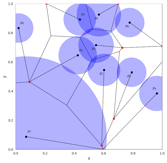
Figure 1: Voronoi Diagram $V(\mathcal{P})$ for a set of 10 randomly allocated points $\mathcal{P}=\{p_{0},p_{1},\dots,p_{9}\}$ in a 2D space. Each red point represents the furthest vertex to each of the points in $\mathcal{P}$ and each circle is the ball of certified positivity given by Proposition II.1.

II-C The LipVor Algorithm

Once the sufficient condition for the positivity certification of a function has been stated in Theorem II.2, it is presented a novel algorithm (LipVor) that, in a finite number of steps, concludes if a function is certified positive or if it is not $\varepsilon$-positive. As mentioned before, by Lemma B.1, for a continuous function in a compact domain, $\varepsilon$-positivity is equivalent to positivity for a specific $\varepsilon$. Consequently, for a sufficiently small $\varepsilon$, concluding that the function is not $\varepsilon$-positive is equivalent to not being positive.

Given a function $f:\Omega\subset\mathbb{R}^{n}\rightarrow\mathbb{R}$ and a set of points $\mathcal{P}=\{p_{1},p_{2},\dots,p_{k}\}\subset\Omega$, if Eq. (3) from Theorem II.2 is not fulfilled, then the initial set of $k$ points $\mathcal{P}$ is not sufficient to guarantee positivity of $f$ in $\Omega$. For example, Figure 1 represents a Voronoi diagram in 2D where Eq. (3) is not fulfilled. Therefore, to try to certify partial monotonicity, LipVor presents a method of selecting points from $\Omega$ that are added to the initial sample $\mathcal{P}$ until Eq. (3) is verified or a counter-example is found.

The idea regarding the LipVor Algorithm 1 is the following. Consider $\mathcal{P}=\{p_{1},p_{2},\dots,p_{k}\}$ a set of points in $\Omega$. The first step of the algorithm is to check that the value of the function at $\mathcal{P}$ is greater or equal than a certain $\varepsilon$. In that case, that would mean that the function fulfills the $\varepsilon$-positivity constraint in $\mathcal{P}$. If for any $p_{j}\in\mathcal{P},\;f(p_{j})<\varepsilon$, then the algorithm would have already found a counter-example. Otherwise, $\varepsilon$-positivity is verified at $\mathcal{P}$ and the next step is to check if the local positivity condition at each point extends to a global positivity condition by Theorem II.2.

In case that Eq. (3) is not satisfied, the LipVor Algorithm iteratively selects a point $p_{k+1}\in\Omega$ to try to fulfill the aforementioned condition. The heuristic of selection of the point $p_{k+1}$ is the following. First of all, for each $p_{j}\in\mathcal{P}$, it is computed the furthest point $v_{j}$ in its Voronoi cell $R_{j}$. As each Voronoi cell is a convex polytope, the distance function attains its maximum in one of the vertex of the polytope. Therefore, to obtain the furthest point $v_{j}$ to the point $p_{j}$ generating the Voronoi cell $R_{j}$, the distance to each vertex of $R_{j}$ is computed.

Once the list of furthest vertices $\mathcal{V}=\{v_{1},v_{2},\dots,v_{k}\}$ of each Voronoi cell is computed, the selection of the point to add next to the Voronoi diagram is made. Each of the furthest vertices $v_{j}$ is related to at least one parent point $p_{j}$ by the relation $v_{j}=\operatorname*{\arg\!\max}_{x\in R_{j}}d(x,p_{j})$. Recall that if $\delta_{j}$ is bigger than the distance of each parent point $p_{j}$ to its furthest vertex $v_{j}$, then the Voronoi cell $R_{j}$ is covered by the ball with center $p_{j}$ and radius $\delta_{j}$. Therefore, starting from $\mathcal{V}$, those vertices already covered by the open ball centered at its parent point are discarded as the corresponding Voronoi cell is already certified positive. Therefore, the list of vertices is reduced to $\mathcal{V}_{p}=\{v_{j}\mid 1\leq i\leq k,\delta_{j}\leq d(p_{j},v_{j})\}$. For instance, in Figure 1, the only regions where $\delta_{j}$ is bigger than the distance from the furthest vertex to the parent point $p_{j}$ are $R_{6}$ and $R_{7}$.

Considering the reduced list of vertices $\mathcal{V}_{p}$, the next point to add to the Voronoi diagram is selected based on the value of $f$ at the parent point $p_{j}$ and the number of adjacent balls ($n_{v_{j}}$) covering the vertex $v_{j}$. The idea of this procedure is to try to fill $\Omega$ with the least number of iterations possible as bigger balls should cover the space faster. As the radius of certified positivity $\delta_{j}=\frac{f(p_{j})}{L}$ is proportional to the value of $f$ at $p_{j}$, by continuity, the expected biggest value of $f$ in $\mathcal{V}_{p}$ is the one corresponding to the biggest value of $f$ in $\mathcal{P}$. Moreover, if the vertex is covered by some of the adjacent balls, the expected non-covered area of the space that could potentially be filled with the added point could be lesser. The way to measure the number of adjacent balls covering the vertex is

$$n_{v_{j}}=|\{p_{l}\mid d(p_{l},v_{j})\leq\delta_{l},\forall\,0\leq l\leq k,l\not=j\}|.$$ (5)

Besides, with probability $0\leq p\leq 1$ the selected vertex $v_{j}$ is the one which correspondent parent $p_{j}$ has the smallest radius and again minimum $n_{v_{j}}$. The idea is to establish a trade-off between exploration and exploitation such as in Reinforcement Learning [37]. Whenever the furthest vertex with the biggest value of the parent $f(p_{j})$ is selected (exploitation) the best option for the next added point is chosen based on the current knowledge. On the other hand, selecting the vertex corresponding to the smallest parent’s value (exploration) corresponds to trying new options that may lead to finding counter-examples. Algorithm 1 depicts the procedure of LipVor.

Algorithm 1 LipVor

  Input: Function $f$, Lipschitz constant $L$, positivity constant $\varepsilon>0$, number of maximum iterations $N$ and a set of points $\mathcal{P}=\{p_{1},p_{2},\dots,p_{k}\}$.

  Output: Bool variable (isPositive) reflecting if $f$ is certified positive or not, counter-example (cExample), if any, and next vertex to be added (nVertex).

  Initialize $\textit{isPositive}=$ True, $\textit{cExample}=$ None, $\textit{nVertex}=$ None, $\textit{counter}=0$, $n_{\min}=\infty$ and $\delta_{\max}=-\infty$.

  Compute the Voronoi diagram $\mathcal{V}(\mathcal{P})=\left(R_{j}\right)_{1\leq j\leq k}$;

  For $n=1\rightarrow N$ do:

       For $j=1\rightarrow\text{length}(\mathcal{P})$ do:

           If $f(p_{j})<\varepsilon$:

                isPositive = False;

                cExample = $p_{j}$;

                Return isPositive, cExample and nVertex

           Else:

                Compute the furthest vertex:

                    $v_{j}=\operatorname*{\arg\!\max}_{x\in R_{j}}d(x,p_{j})$;

                Compute the distance to the furthest vertex:

                    $d_{j}=d(p_{j},v_{j})$;

                If $\delta_{j}=\frac{f(p_{j})}{L}\leq d_{j}$:

                    Using Eq. (5) find $n_{j}$;

                    If $\delta_{j}\geq\delta_{\max}$ and $n_{j}\leq n_{\min}$:

                        $n_{\min}=n_{j}$;

                        $\delta_{\max}=\delta_{j}$;

                        $\textit{nVertex}=p_{j}$;

                        isPositive = False;

                Else :

                    counter +=1

        If $\textit{counter}=\text{length}(\mathcal{P})$:

            Return isPositive, cExample and nVertex

       End for

       Add point nVertex to $\mathcal{P}$;

       Compute new Voronoi diagram $\mathcal{V}(\mathcal{P})$;

  End for

  Return isPositive, cExample and nVertex.

In practice, the LipVor Algorithm is slightly modified to find not just one counter-example but a list of them. The idea is to expand not just the probably biggest and least covered vertices but also those whose parent’s evaluation is lower than $\varepsilon$ and the value is the smallest (biggest in absolute value). Consequently, even if for any $p_{j}\in\mathcal{P},f(p_{j})<\varepsilon$, the point $p_{j}$ is also considered as a valid parent to find its furthest vertex. Therefore, the LipVor Algorithm would also expand the subdomain where the positivity is not verified. Hence, when using the LipVor Algorithm to certify if a function fulfills a positivity condition, it can return whether the function is positive and the subdomains where the condition is certified met and where it is not.

As stated in the pseudocode, the LipVor Algorithm ends in a finite number of $N$ steps. The following Theorem II.3 shows that a value of $N$ can always be chosen depending only on $\Omega$, $\varepsilon$ and $L$ so that LipVor always reaches a definitive conclusion within the given number of iterations. A complete proof of Theorem II.3 is given in appendix B.

Theorem II.3.

Under the aforementioned conditions, the LipVor Algorithm concludes in a finite number of steps. Moreover, the maximum number of steps $N$ that the LipVor Algorithm needs to certify that a function $f$ is positive or to find a counter-example can be upper bounded by

$$N\leq\frac{\operatorname{Vol}(\bar{\Omega})}{\operatorname{Vol}\left(B\left(\frac{\varepsilon}{2L}\right)\right)},$$ (6)

where $\bar{\Omega}$ is the domain extended by $\frac{\varepsilon}{2L}$ and $B\left(\frac{\varepsilon}{2L}\right)$ is a ball of radius $\frac{\varepsilon}{2L}$.

As observed, $N$ depends on the selected $\varepsilon$. Therefore, after the LipVor Algorithm has reached the maximum number of iterations $N$ or it is stopped because it is verified the sufficient condition stated in Eq. (3), the function $f$ is certified positive (if $\textit{isPositive}=$ True) or certified not $\varepsilon$-positive (if $\textit{cExamples}\not=$ None or $\textit{cExamples}=$ None and $\textit{isPositive}=$ False). However, as mentioned before, considering $\varepsilon$-positive is not a restrictive constraint as any positive function in a compact domain is $\varepsilon_{f,\Omega}$-positive for a specific $\varepsilon_{f,\Omega}$. Therefore lowering sufficiently $\varepsilon$, any positive function becomes $\varepsilon$-positive. Consequently, considering $\varepsilon$-positivity is just a formal convention to establish Eq. (6).

As a final remark, as stated in appendix B, Eq. (6) can be upper bounded by

$$N\leq\frac{\operatorname{Vol}(\bar{\Omega})}{\operatorname{Vol}\left(B\left(\frac{\varepsilon}{2L}\right)\right)}\leq\left(\frac{2\cdot\left(a\cdot L+\varepsilon\right)}{\pi^{\frac{1}{2}}\cdot\varepsilon}\right)^{n}\Gamma\left(\frac{n}{2}+1\right),$$

where $\Gamma$ is the gamma function and $a$ is a constant dependent on the size of the domain $\Omega$.

III Certification of Partial Monotonicity for ANNs

III-A Partial Monotonicity of an ANN

As previously mentioned in Section I, partial monotonicity of a function $g$ w.r.t. the $r^{th}$ input, with $0\leq r\leq n$, can be formulated as a positivity constraint over the partial derivative $g_{x_{r}}$. Mathematically, a function $g:\Omega\subseteq\mathbb{R}^{n}\rightarrow\mathbb{R}$ is strictly increasing (resp. decreasing) partially monotonic w.r.t. the $r^{th}$ input if

$$g(x_{1},\dots,x_{r},\dots,x_{n})<g(x_{1},\dots,x^{\prime}_{r}\dots,x_{n})\,,\forall\ x_{r}<x^{\prime}_{r}\,$$ (7)

$$(\text{resp.}\;g(x_{1},\dots,x_{r},\dots,x_{n})>g(x_{1},\dots,x^{\prime}_{r}\dots,x_{n})).$$

Consequently, a function $g$ will be partially monotonic w.r.t. a set of features $\{x_{i_{1}},\dots,x_{i_{k}}\}$ wih $k\leq n$ whenever Eq. (7) is verified for each $i_{j}$ simultaneously with $j\in\{1,\dots,k\}$.

Therefore, considering a function $g:\Omega\subseteq\mathbb{R}^{n}\rightarrow\mathbb{R}$ with $g\in C^{1}(\Omega)$, if $g_{x_{r}}(x)>0$ (resp. $g_{x_{r}}(x)<0$) the function $g$ is strictly increasing (resp. decreasing) partially monotonic w.r.t. the $r^{th}$ input feature at the point $x\in\Omega$. Moreover, whenever $g_{x_{r}}(x)\geq\varepsilon$ ($g_{x_{r}}(x)\leq-\varepsilon$), the function $g$ is increasing (decreasing) partially $\varepsilon$-monotonic. Consequently, the methodology stated in Section II can be applied to certify partial monotonicity of a function $g\in C^{1,1}(\Omega)$ (differentiable and with L-Lipschitz partial derivatives) by just taking $f:=g_{x_{r}}$.

On the other hand, ANNs, specifically feedforward neural networks, are composed of interconnected layers of neurons that process and transform data. Therefore, an ANN $g:\Omega\subseteq\mathbb{R}^{n}\rightarrow\mathbb{R}$ with $K$ layers and $n^{l}$ neurons in the l-layer, with $0<l\leq K$, can be mathematically described as a composition of point-wise multiplication with non-linear activation functions, such that the output of the $l^{th}$ layer $o^{l}$ is given by

$$o^{0} =\mathbf{x},$$

$$z^{l} =o^{l-1}\cdot W^{l}+b^{l}\quad\text{for }l=1,2,\ldots,K,$$ (8)

$$\ o^{l} =\varphi^{l}\left(z^{l}\right),\quad\text{for }l=1,2,\ldots,K,$$ (9)

$$y =g(\mathbf{x};\mathbf{W},\mathbf{b})=\varphi^{K}\left(\mathbf{o}^{K-1}\cdot W^{K}+b^{K}\right),$$ (10)

where $\mathbf{x}$ represents the input data, $W^{l}\in\mathbb{R}^{n^{l-1}}\times\mathbb{R}^{n^{l}}$, $b^{l}\in\mathbb{R}^{n^{l}}$ and $\varphi^{l}(\cdot)$ are the weights, bias and activation function of the $l^{th}$ layer respectively.

In particular, ANNs using $C^{2}(\Omega)$ activation functions, such as Sigmoid, Tanh, etc., are $C^{1,1}(\Omega)$ functions in a compact domain $\Omega$. Therefore, knowing an upper bound of the Lipschitz constant of the partial derivatives of an ANN, it is possible to pose the partial monotonicity certification problem as an application of the LipVor Algorithm to the partial derivatives. Consequently, it is crucial to compute an upper bound $\hat{L}$ of the Lipschitz constant $L$ of the partial derivatives of an ANN.

Without loss of generality, in the following methodology, the ANN is going to be considered strictly increasing partially monotonic w.r.t. the $r^{th}$ input. Subsequently, when dealing with multiple monotonic features, the procedure remains the same by simply considering the minimum radius among each of the monotonic features. By using this minimum radius as the ball’s radius, we ensure monotonicity is preserved for each monotonic feature. Conversely, if there exists a point $p_{j}$ where the constraint is not satisfied for any of the monotonic features, a radius $\delta_{j}=\frac{g_{x_{i}}(p_{j})}{L_{j}}$ is computed for each unsatisfied constraint and the maximum of these radii is used. This maximum radius represents the largest radius within which some of the monotonicity conditions are not met. Moreover, the methodology could be extended to vector-valued ANN $g:\mathbb{R}^{n}\rightarrow\mathbb{R}^{m}$ considering each of the components from the codomain $g^{i},i\in\{1,2,\dots,m\}$.

III-B Lipschitz Constant Estimation of the Partial Derivative of an ANN

As mentioned in Section I, the study of estimations of the Lipschitz constant of an ANN has already been conducted, but this was not the case for the Lipschitz constant of the partial derivative of an ANN. This study presents a novel approach to computing an upper bound for such Lipschitz constant.

Recall that if $f$ is an L-Lipschitz function $f\in C^{0,1}(\Omega_{C})$ in a compact convex domain $\Omega_{C}$ then the Lipschitz constant of $f$ in $\Omega_{C}$ is the maximum norm of its gradient. This result, stated in the following proposition, could be enunciated more generally but for simplicity, it is presented for differentiable functions with codomain $\mathbb{R}$ (cf. Thm. 3.1.6 [35, Rademacher]).

Proposition III.1.

Let $\Omega_{C}\subseteq\mathbb{R}^{n}$ a compact convex domain and $f:\Omega_{C}\rightarrow\mathbb{R}$ a $C^{1}(\Omega_{C})$ function. Then

$$L=\sup_{x\in\Omega_{C}}\left\lVert\nabla f(x)\right\rVert,$$

where $\nabla f(x)$ is the gradient of the function $f$.

Considering now an ANN $g:\Omega_{C}\subseteq\mathbb{R}^{n}\rightarrow\mathbb{R}$ with $\Omega_{C}$ a compact convex domain and $g\in C^{1,1}(\Omega)$, then, applying Proposition III.1 to the $r^{th}$ partial derivative $g_{x_{r}}$ of the ANN, the Lipschitz constant is obtained as the maximum norm of $\tilde{H}_{g}$ where

$$\tilde{H}_{g}=\left(\frac{\partial g}{\partial x_{r}\partial x_{j}}\right)_{j},\forall\;1\leq j\leq n,$$

is the Hessian of the output of $g$ w.r.t. the $r^{th}$ input. Hence by Proposition III.1,

$$L=\sup_{x\in\Omega}\left\lVert\nabla g_{x_{r}}(x)\right\rVert=\sup_{x\in\Omega}\left\lVert\tilde{H}_{g}(x)\right\rVert.$$

Consequently, an upper bound of $\left\lVert\tilde{H}_{g}\right\rVert$ establishes an upper estimation $\hat{L}$ of the Lipschitz constant $L$ of the $r^{th}$ partial derivative of an ANN.

To generate an upper bound of $\left\lVert\tilde{H}_{g}\right\rVert$, it is going to be used that an ANN with K-layers can be described as a composition of activation functions and linear transformations (Eq. (8)-(10)). Therefore, considering

$$H_{0}^{l}=\left(\frac{\partial^{2}o^{l}_{k}}{\partial x_{i}\partial x_{j}}\right)_{i,j,k},\,\forall\,1\leq i,j\leq n^{0},1\leq k\leq n^{l},$$ (11)

the Hessian of the $l^{th}$ layer w.r.t. the input layer (layer 0), then, by Eq. (10),

$$\tilde{H}_{g}=\tilde{H}_{0}^{K}=\left(\frac{\partial^{2}o^{K}}{\partial x_{r}\partial x_{j}}\right)_{j},\,\forall\,1\leq j\leq n^{0}.$$

Therefore, the maximum norm of the Hessian of the $k^{th}$ layer of the ANN w.r.t. the $r^{th}$ input ($L_{x_{r}}^{K}$) can be recursively upper bounded using the weights of the preceding layers $W^{l}$, the Hessian of the $K^{th}$ layer

$$H_{K}^{K}=\left(\frac{\partial^{2}o^{K}}{\partial z_{i}\partial z_{j}}\right)_{i,j},1\leq i,j\leq n^{K-1}$$

with respect to $z^{l}$ (Eq. (8)) and the upper bound of the $K-1$ layer $\hat{L}_{x_{r}}^{K-1}$ as follows.

Theorem III.2.

Let $g:\Omega\subseteq\mathbb{R}^{n}\rightarrow\mathbb{R}$ be an ANN with K-layers, then the Lipschitz constant $L_{x_{r}}^{K}$ of the $r^{th}$ partial derivative $g_{x_{r}}$ of an ANN verifies that

$$L_{x_{r}}^{K}\leq\hat{L}_{x_{r}}^{K}:=\max|a_{k}^{K}|\cdot\lVert W_{1j}^{1}\rVert\cdot\lVert W^{1}\rVert\cdot\lVert W^{2}\rVert^{2}\dots\lVert W^{K}\rVert^{2}\\ +\hat{L}_{x_{r}}^{K-1}\cdot\lVert W^{K}\rVert,$$ (12)

where $W^{k}$ is the weight matrix of the $k^{th}$ layer, $W_{1j}^{1}$ is the first row of the weight matrix $W^{1}$, $\hat{L}_{x_{r}}^{K-1}$ is the upper bound of Lipschitz constant of the $r^{th}$ partial derivative of the $K-1$ layer of the ANN and $a_{k}^{K}=\|H_{K}^{K}\|_{\infty}:=\max_{1\leq i\leq n}\left(\sum_{j=1}^{n}\left(H_{K}^{K}\right)_{i,j}\right)$.

A complete proof of Theorem III.2 can be found in appendix C.

Finally, it is important to acknowledge that for the most commonly used activation functions in neural networks, the second derivative is upper bounded by 1. For example, in the case of the sigmoid activation function, the second derivative is given by $\sigma^{\prime\prime}(x)=\sigma^{\prime}(x)(1-2\cdot\sigma(x))$, which is clearly upper bound by 1. Moreover, note that the aforementioned theorem is valid for vector-valued ANNs $g:\mathbb{R}^{n}\rightarrow\mathbb{R}^{m}$ as Eq. (12) is recursively obtained using the upper bound of the intermediate layers which are vector-valued functions with codomain’s dimension the number of neurons in the intermediate layer.

IV Extension: Training Certified Monotonic Neural Networks

This section presents the proposed methodology to train unconstrained probably partial $\varepsilon$-monotonic ANNs that could later be certified as partial monotonic using the LipVor Algorithm. The idea is to use a modified version of the usual training loss, similar to [24]. In this case, the ANN is forced to follow an $\varepsilon$-monotonic relationship at the training data by means of a penalization term. Therefore, by continuity of the ANN, enforcing a $\varepsilon$-monotonic constraint at the training data, it is expected that in a neighbourhood of every training point, the ANN is partially monotonic. However, as concluded in [24], partial monotonicity is only expected to be achieved close to the regions where it is enforced. Therefore, there is no guarantee (a priori) of obtaining a partial monotonic ANN in the whole domain $\Omega$. Consequently, after training the unconstrained partial $\varepsilon$-monotonic ANNs, it is computed the LipVor Algorithm to try to certify partial monotonicity. Hence, by applying this methodology, it is possible to certify partial monotonicity without needing to use constrained architectures.

Considering an ANN $g:\Omega\subseteq\mathbb{R}^{n}\rightarrow\mathbb{R}$, to find the optimum ANN’s parameters, an optimization procedure to minimize a loss function is followed. The loss function is intended to measure the difference between the real output values $y$ and the predicted $\hat{y}$ ones. Therefore, the loss funtion of the ANN can be stated as

$$\mathcal{L}(\mathbf{W},\mathbf{b};\mathcal{D})=\sum_{(\mathbf{x},\mathbf{y})\in\mathcal{D}}\ell\left(y,g(\mathbf{x};\mathbf{W},\mathbf{b})\right),$$

where $\mathbf{W}$ and $\mathbf{b}$ denote the weights and biases of the neural network, $\mathcal{D}$ is the dataset containing input-output pairs $(\mathbf{x},y)$ and $\ell$ is the loss function that measures the discrepancy between the predicted output and the actual output. For regression problems, the loss function is usually the sum of squared errors, while for classification problems, the maximum likelihood.

During the optimization process, the ANN is guided through gradient descent towards the parameters that minimize the loss function. The gradient of the loss function w.r.t. the parameters is efficiently computed by the backpropagation algorithm. Consequently, an ANN can be guided to follow a specific partial $\varepsilon$-monotonic relation w.r.t. the $r^{th}$ input, with $\varepsilon>0$, between the explanatory and the response variables by adding, to the loss function, a regularization term that penalizes the objective if the $\varepsilon$-monotonic relation is not fulfilled. Therefore, it is considered a modified loss function $\tilde{\mathcal{L}}$, encompassing the partial $\varepsilon$-monotonic constraint,

$$\tilde{\mathcal{L}}(\mathbf{W},\mathbf{b};\mathcal{D})=\mathcal{L}(\mathbf{W},\mathbf{b};\mathcal{D})+\lambda\Omega_{g,r}(\mathcal{D},\varepsilon),$$

where $\mathcal{L}(\mathbf{W},\mathbf{b};\mathcal{D})$ is the original loss function, $\mathcal{D}$ is the training dataset and the term $\Omega_{g,r}$ is the $\varepsilon$-monotonic penalization based on the $r^{th}$ column of the Jacobian matrix . On the other hand, the coefficient $\lambda$ is used to scale the regularization term, thereby adjusting its strength.

To compute the penalization term, it is computed the sum of the values of the $r^{th}$ column where the partial $\varepsilon$-monotonic constraint is not followed. Therefore, if the relation is increasing (decreasing) $\varepsilon$-monotonic, then the rectified values of the negative (positive) sum of the Jacobian matrix and $\varepsilon$ are summed up. Consequently, the regularization term is computed as

$$\Omega_{g,r}(\mathcal{\bar{D}},\varepsilon)=\sum_{x\in\mathcal{\bar{D}}}\left[\max\left(0,-J_{r}(\mathbf{x})+\varepsilon\right)\right],$$

where $J_{r}$ represents the $r^{th}$ column of the Jacobian matrix evaluated at $\mathbf{x}$ $\left(\text{i.e.,}\quad J_{r}=\frac{\partial g}{\partial x_{r}}\right)$. Considering this strategy, the parameters’ optimization will be guided towards ensuring that the partial $\varepsilon$-monotonic constraint is fulfilled for all data samples in $\mathcal{D}$.

Once the training process has concluded, the LipVor Algorithm is executed to certify if the ANN is partially monotonic. If the LipVor Algorithm concludes that the ANN is not partially $\varepsilon$-monotonic and finds some counter-examples, these points will be used as an external dataset where the partial $\varepsilon$-monotonic penalization is also enforced. Therefore, it is added a penalization in a subdomain where the trained ANN is not partially $\varepsilon$-monotonic. This approach is an improvement compared to [24] as the penalization term is not computed at random points but at counter-examples where the ANN is not $\varepsilon$-monotonic. Consequently, it is expected that after fine-tuning the trained ANN, at the external points combined with the training data, the ANN can be certified partially monotonic by the LipVor Algorithm. Therefore, this methodology can be applied iteratively until converging to a partial monotonic ANN.

Besides, to avoid overfitting, it is considered an early stopping criterion where the training is stopped after $N_{p}$-epochs without improvement. The number of consecutive epochs $N_{p}$ during which the validation loss fails to decrease before terminating the training is referred to as patience. Moreover, the early stopping criteria is considered a valid early stopping epoch whenever the penalization loss associated with the partial $\varepsilon$-monotonic constraint is 0. Therefore, the ANN is partial $\varepsilon$-monotonic in the training data, and consequently, it is reasonable to attempt to verify partial monotonicity in $\Omega$.

V Case Studies

In the following section, two case studies where partial monotonicity constraints should be enforced are presented. In the first case, an ANN is used to estimate the heat transfer of a 1D bar. As the input domain is 2 dimensional, it will allow us to visualize the Voronoi expansion and the partial monotonicity certification using the LipVor Algorithm. The second case is a four-dimensional dataset where partial monotonicity aligns with ethical predictions. Therefore, this dataset is an example of how partial monotonicity ensures ethical fairness and the application of LipVor to an input multidimensional domain. Consequently, these two experiments constitute real-world scenarios where partial monotonicity aligns with physics or ethical principles respectively.

V-A Case Study: Heat Equation

Accurately modeling mechanical behavior based on observed data is vital for predictive maintenance and digital twin development [39]. However, capturing complex relationships in dynamic systems remains a challenge [40]. Traditional approaches often fall short, necessitating advanced techniques like ANNs [41]. Yet, ensuring that ANNs align with physical laws is crucial. This approach not only enhances predictive accuracy but also ensures that the approximated solution by the ANN adheres to fundamental principles [42]. For instance, when considering the temperature evolution of a solid being heated, it should respect some physical laws described by the heat equation. However, the trained ANN could be overfitting and consequently not respecting the aforementioned physical principles.

Expanding on the necessity of preserving physical principles within ANNs, this case study presents an example of a physical property of the heat equation in a 1D rod encoded as a partial monotonic constraint. The heat equation is a fundamental partial differential equation (PDE) in mathematical physics that describes heat’s distribution in a given medium over time. In its simpler form, the PDE can be mathematically expressed as $u_{t}=k\cdot u_{xx}$, where $u(x,t)$ represents the temperature distribution as a function of space ($x$) and time ($t$), and $k$ is the thermal diffusivity constant. Consequently, ensuring that the ANN is partially monotonic entails respecting a physical principle.

Dirichlet boundary conditions (BC) are often employed alongside the heat equation to specify the temperature behavior at the medium’s boundaries. An instance of such a condition is when the temperature at the boundaries grows linearly with time, representing a situation where heat is constantly being added or removed from the system at a fixed rate. In this case, time-dependent Dirichlet BC will be used for a 1D rod of length $L$. Formally, the heat equation with the aforementioned time-dependent Dirichlet BC can be described as

$$\left\{\begin{aligned} &\frac{\partial u}{\partial t}=k\cdot\frac{\partial^{2}u}{\partial x^{2}},\quad\text{for }0<x<L,\quad t>0\\ &u(0,t)=t,\quad\\ &u(L,t)=t,\quad\\ &u(x,0)=0.\quad\end{aligned}\right.$$ (13)

Under this BC, the heat equation (13) is an example of a 2D problem where the solution is partially monotonic w.r.t. the input $t$ . Therefore, enforcing the partial monotonic constraint aligns with the expected physical properties of the solution.

Acquiring experimental data for physical phenomena is often a costly and error-prone process due to sensor measurement inaccuracies [40]. Consequently, physical datasets tend to be limited in size and exhibit significant noise presence. Therefore, to generate a realistic synthetic scenario, 30 random measures of the temperature $u(x,t)$ distribution of a 1D rod with length $L=1$ with noise, following $\mathcal{N}(0,0.02)$, have been sampled (Fig 2).

Consequently, the generated dataset has 30 pairs of (space, time) and temperature $\{(x,t);u(x,t)\}$ as input/output values. Adding noise to the simulated solution $u(x,t)$ effectively perturbs the simulated temperature measurements, introducing variability akin to practical measurement uncertainties encountered in real-world scenarios. Additionally, for model training and evaluation, the dataset is divided into training, validation, and testing subsets following an initial $80/20$ split, with $20\%$ of the samples allocated for testing purposes and the remaining $80\%$ divided again in a $80/20$ split in training and validation.

It is worth mentioning that multiple experiments where executed with different seeds and for most of the generated datasets the unconstrained ANN is certified partial monotonic after enforcing the penalization term. However, in order to exemplify the worst case scenario, this case study presents an example where the unconstrained ANN with the aforementioned penalization term did not converge directly to a partial monotonic solution. Therefore, this case study exemplifies the proposed iterative methodology to converge to a partial monotonic ANN.

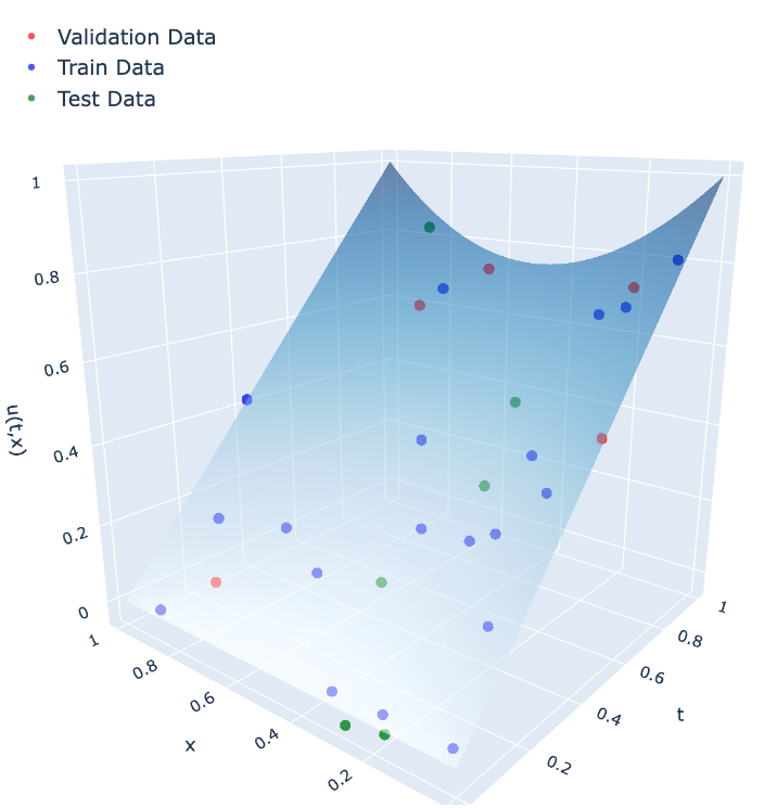
Figure 2: Surface of the solution of the heat equation (13) and the training (blue), validation (red) and test (green) datasets obtained from the solution with added noise.

Considering the ANN architecture, given the limited number of training samples, a feedforward ANN with 1 hidden layer and 10 neurons with a hyperbolic tangent (tanh) activation function has been considered. Moreover, L-BFGS has been selected as the optimizer with a learning rate of $0.01$. Besides, a penalization of $\lambda=0.1$ has been imposed to guide the training towards a $\varepsilon$-monotonic solution taking $\varepsilon=0.1$. The maximum number of epochs for the training process was fixed at 5000 with a patience of $N_{p}=1000$ epochs for the early stopping.

After the training process is completed, the LipVor Algorithm is used to determine if the ANN is partially $\varepsilon$-monotonic w.r.t. $t$ in $\Omega$. As illustrated in Figure 3(a), the partial derivative of the trained ANN w.r.t. input $t$ is not positive in the whole $\Omega$. Specifically, whenever $t\approx 0$ and $x\in[0.5,0.6]$ the partial derivative is negative. Therefore, it is expected that the LipVor Algorithm is able to effectively find counter-examples in the aforementioned region.

Following the bound proposed in Theorem III.2, it is obtained a Lipschitz estimation of $\hat{L}=17.58$. Moreover, to start the LipVor Algorithm, the points from the training dataset are selected to initialize the algorithm, and a maximum number of 700 iterations is fixed (Figure 3(b)). As observed in Figure 3(c), after 22 iterations the LipVor Algorithm has effectively detected the first counter-example. Moreover, after reaching the maximum number of iterations (Figure 3(d)), 36 counter-examples of partial $\varepsilon$-monotonicity have been detected in contrast with the certified area which corresponds to the $66.2\%$ of $\Omega$.

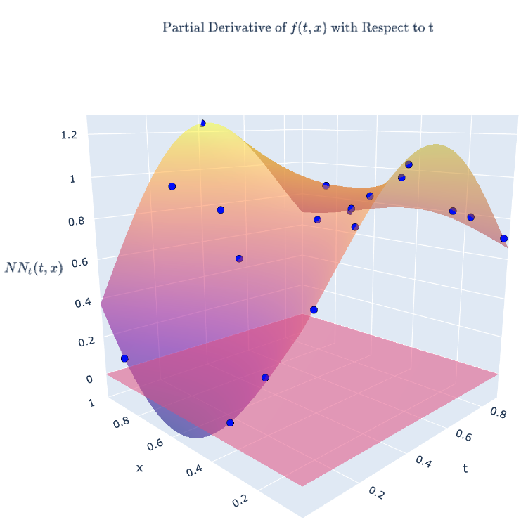
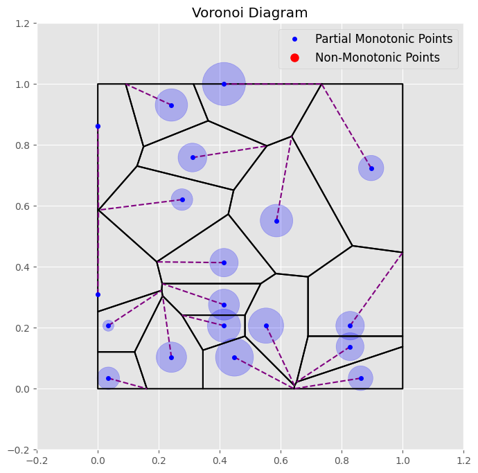
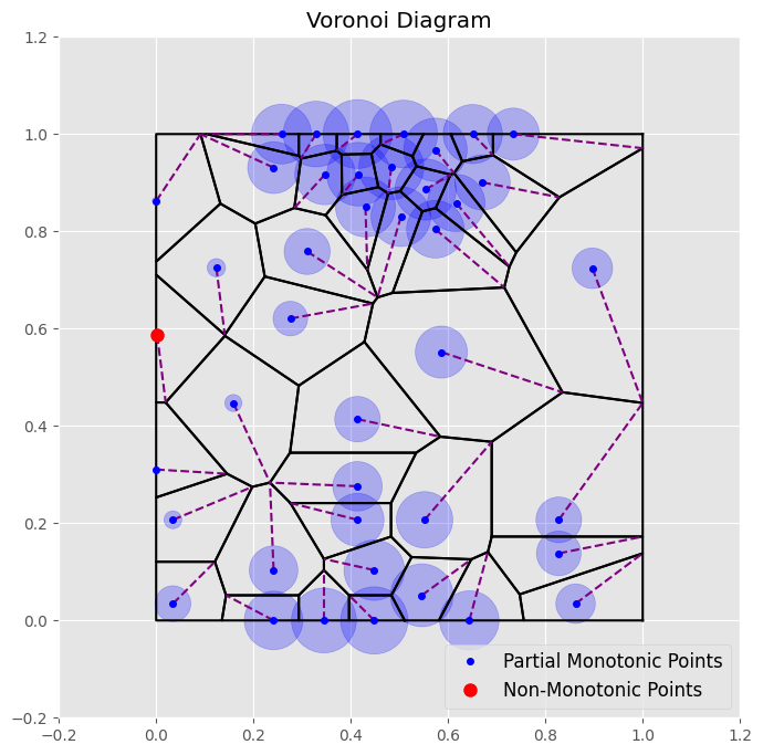
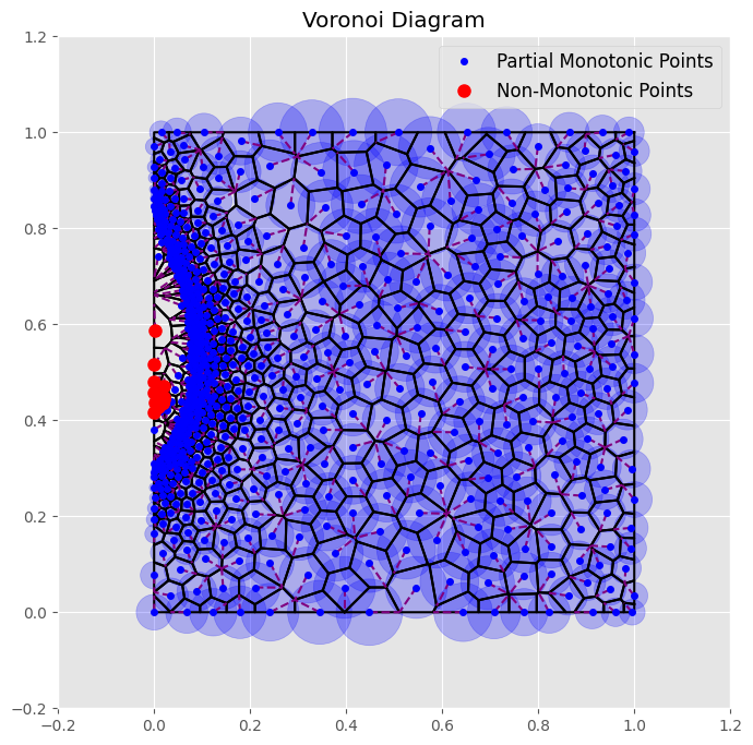
Figure 3: Evolution of the Voronoi diagram generated by the LipVor Algorithm. (a) Evaluation of the partial derivative of the ANN w.r.t. the input $t$ in the domain. (b) Initialization of the Voronoi diagram using the training set. (c) Voronoi diagram expansion when the first counter-examples is detected by the LipVor Algorithm. (d) Final iteration, after LipVor has reached the maximum number of steps, showing the partial monotonic subdomain and the found counter-examples.

Once the LipVor Algorithm has proved that the initial ANN is not partially $\varepsilon$-monotonic, based on the found counter-examples, the ANN is fine-tuned. The initial ANN demonstrated a training MAE of $9.06\times 10^{-3}$ and a test MAE of $1.66\times 10^{-2}$, with corresponding $R^{2}$ values of 0.9984, and 0.9942. After fine-tuning, the ANN showed a training MAE of $1.17\times 10^{-2}$ and a test MAE of $1.58\times 10^{-2}$. The $R^{2}$ values for the fine-tuned ANN were 0.9970 for training and 0.9950 for testing. These results indicate that the fine-tuning process slightly improved the test set performance, enhancing the model’s ability to generalize to new data.

Once the training is completed, the LipVor Algorithm is executed again to certify if the ANN is now partially monotonic. As observed in Figure 4, the partial derivative of the ANN w.r.t. the $t$ input is positive in $\Omega$ and the LipVor Algorithm converges after 581 iterations. Therefore the fine-tuned ANN is certified partially monotonic in $\Omega$.

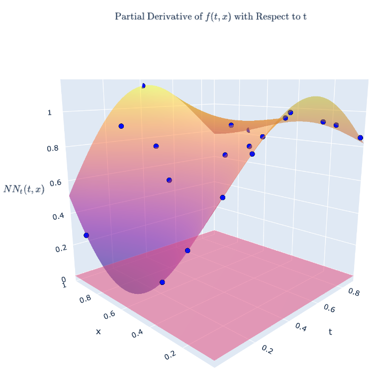
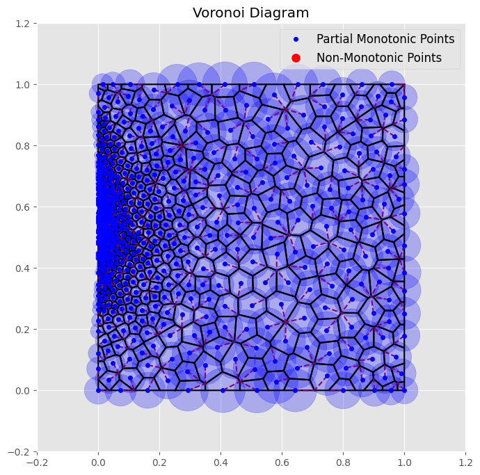
Figure 4: Partial monotonicity verification of the ANN using the LipVor Algorithm. (a) Evaluation of the partial derivative of the ANN w.r.t. the input $t$ in the domain. (b) Visualization of the Voronoi Diagram generated by the LipVor Algorithm after certifying partial monotonicity.

V-B Case Study: Ethical Monotonic Predictions for the ESL dataset

The Employee Selection (ESL) dataset [43] comprises profiles of candidates applying for specific industrial roles. The four input variables are scores, from 1 up to 9, assigned by expert psychologists based on the psychometric test outcomes and candidate interviews. The output presents an overall score on an ordinal scale from 1 to 9, indicating the extent to which each candidate is suitable for the job. As stated in [44], the ESL dataset is one of the benchmarks in the literature on monotonic datasets. Each four variables are monotone as a better performance in a psychometric test should be reflected in an increased overall score. Therefore, a model violating the monotonic constraint would be generating unethical predictions penalizing a candidate for having a better psychometric test.

The dataset is comprised of four input variables and a total of 488 instances. Within these instances, 75$\%$ (366 instances) have been further divided into a 75/25 split for training (274 instances) and validation (92 instances) purposes. The remaining 25$\%$ (122 instances) has been allocated for testing. As mentioned before, the four input variables have values ranging in $[1,9]$. Therefore, the inputs are min-max scaled to transform each variable to $[0,1]$ so the inputs domain is $\Omega=[0,1]^{4}\subset\mathbb{R}^{4}$.

An ANN with an architecture of 2 hidden layers with 5 neurons in each layer is trained. The activation function selected for each neuron is tanh. In this case, an Adam optimizer has been chosen with a learning rate of $0.001$. Moreover, to regularise the ANN, it has been considered a weight decay of $0.005$. The proposed strength of the penalization $\lambda$ is $0.1$ and the ANN is trained considering $\varepsilon$-monotonicity with $\varepsilon=0.1$. The training process was set to run for a maximum of 5000 epochs, with a patience $N_{p}=1000$ epochs. The training process ended after 2298 epochs obtaining the results presented in Table I in training, validation and test sets.

TABLE I: Training and Test MSE and $R^{2}$ results for the trained ANN

	Training	Validation	Test
MAE	0.05356	0.04399	0.05444
$R^{2}$	0.82696	0.90176	0.83488

After the training comes to an end, the LipVor Algorithm is used to check whether the trained ANN is monotonic w.r.t. the four input variables. In this case, the Lipschitz estimation is $\hat{L}=0.91$ and the LipVor Algorithm is computed starting from 10 random points chosen from the training set. After 423 iterations, the LipVor Algorithm certifies that the whole input space $\Omega$ is covered and, therefore, the trained ANN is provably monotonic w.r.t. the input variables.

VI Conclusions

In this article, it is proposed a novel algorithm (LipVor) to certify if a black-box model fulfills a positivity condition based on the Lipschitzianity of the model function. In particular, the partial monotonicity of an ANN can be stated as a positivity condition of the partial derivatives of the ANN. Therefore, it is possible to apply the LipVor Algorithm to mathematically certify if an ANN is partially monotonic or find counter-examples. To do so, it is also presented an upper bound of the Lipschitz constant of the partial derivatives of an ANN.

The obtained results underscore that using the LipVor Algorithm opens up new possibilities in sectors, such as the banking sector, where regulatory agencies require ethical predictions posed as partial monotonic constraints. Furthermore, many problems, such as the convexity of an ANN, can be formulated as a positivity constraint and consequently, the LipVor Algorithm could be used to certify other properties from an ANN provably. Moreover, the methodology presented could be extended to other ANN architectures such as convolutional neural networks or other feed-forward layers such as normalization layers. Besides, it is proposed as future research its extension to recurrent neural networks or transformers.

Appendix A Proof of Theorem II.2

This appendix presents a proof of Theorem II.2, that states a sufficient condition for an L-Lipschitz function $f:\Omega\subseteq\mathbb{R}^{n}\rightarrow\mathbb{R}$ to be certified positive in $\Omega$. First of all, let us present a technical lemma that will allow us to check if a union of balls $\bigcup_{i\in I}B(p_{i},\delta_{i})$ covers $\Omega$.

Lemma A.1.

Let $\Omega\subset\mathbb{R}^{n}$ be a compact domain and $\mathcal{P}=\{p_{1},p_{2},\dots,p_{k}\}$ a set of points defining a Voronoi diagram with cells $(R_{i})_{i\in I}$, with $I=\{1,\dots,k\}$, if $\forall\,p_{j}\in\mathcal{P}$ it is verified that

$$\max_{x\in R_{j}}d(x,p_{j})<\delta_{j},$$

for some $\delta_{j}$ with $j\in I$, then

$$\Omega\subseteq\bigcup_{i\in I}B(p_{i},\delta_{i}).$$

Proof.

Let us prove the lemma by contradiction. Let us suppose that there exists $x^{*}\in\Omega$ such that $x^{*}\not\in\bigcup_{i\in I}B(p_{i},\delta_{i})$.

By definition of the Voronoi diagram in a compact space $\Omega$, there exists at least one $p_{j}\in\mathcal{P}$ such that $x^{*}\in R_{j}$. On the other hand, as $x^{*}\not\in\bigcup_{i\in I}B(p_{i},\delta_{i})$, then $d(x^{*},p_{j})>\delta_{j}$. Therefore

$$d(x^{*},p_{j})>\delta_{j}>\max_{x\in R_{j}}d(x,p_{j}),$$

which is a contradiction with the initial supposition. ∎

Recall that Proposition II.1 states that if $f:\Omega\subset\mathbb{R}^{n}\rightarrow\mathbb{R}$ is an L-Lipschitz function such that $f(x_{0})>0$, with $x_{0}\in\Omega$, then there exists a radius $\delta_{0}=\frac{f(x_{0})}{L}$ of certified positivity verifying that $f(x)>0,\;\forall\;x\in B(x_{0},\delta_{0})$. Therefore, given a set of points $\mathcal{P}=\{p_{1},p_{2},\dots,p_{k}\}$ and an L-Lipschitz function $f$, the previous lemma can be used to state a sufficient condition for $f$ to be certified positive based on the evaluations at $\mathcal{P}$. Specifically, it suffices to check if the furthest point from each Voronoi cell to the point defining the cell, is smaller than the radius of certified positivity given by Proposition II.1.

Theorem A.2.

Let $\Omega\subset\mathbb{R}^{n}$ be a compact domain, $\mathcal{P}=\{p_{1},p_{2},\dots,p_{k}\}$ a set of points contained in $\Omega$ and $V(\mathcal{P})=(R_{j})_{j\in I}$ be the Voronoi diagram of $\mathcal{P}$. Let $f:\Omega\rightarrow\mathbb{R}$, with $f\in C^{0,1}(\Omega)$, an L-Lipschitz function and let $\delta_{j}=\frac{f(p_{j})}{L},\;\forall j\in I=\{1,2,\dots,k\},$ be the radius of certified positivity given by Proposition II.1. Then if

$$\max_{x\in R_{j}}d(x,p_{j})<\delta_{j}\;\forall j\in I$$ (14)

the function $f$ is positive in $\Omega$.

Proof.

Let $x$ be a point in the compact domain $\Omega$ and suppose that $f$ verifies Eq. (14). Therefore, by Lemma A.1,

$$\Omega\subseteq\bigcup_{i\in I}B(p_{i},\delta_{i}).$$

Consequently, by definition of the Voronoi diagram, there exists a Voronoi cell $R_{j}$ such that $x\in R_{j}\subseteq B(p_{j},\delta_{j})$. Therefore, by Proposition II.1, $f(x)>0$. Consequently, f is positive in the whole compact domain $\Omega$. ∎

Appendix B Proof of Theorem II.3

Recall that the LipVor Algorithm provides a mathematical certification to check if a function $f$ is positive in a compact domain $\Omega$. As mentioned in section II-C, one aspect worth mentioning is the finiteness of the LipVor Algorithm. Therefore, in this appendix, it is proven Theorem II.3 that states that the LipVor Algorithm reaches a conclusion in a finite number of steps and gives an upper bound of the maximum number of iterations needed.

Let us start by recalling the definition of $\varepsilon$-positivity that will be later used in Theorem B.2. Let $f:\Omega\subseteq\mathbb{R}^{n}\rightarrow\mathbb{R}$ be a function in a domain $\Omega$, then, it is said that $f$ is $\varepsilon$-positive, with $\varepsilon>0$, if

$$f(x)\geq\varepsilon,\forall\;x\in\Omega.$$

Although $\varepsilon$-positivity might seem like a more restrictive condition than positivity, the following lemma will prove that every positive function in a compact domain $\Omega$ is indeed $\varepsilon$-positive for some $\varepsilon$. Moreover, it is trivial that an $\varepsilon$-positive function is positive. Therefore, for continuous functions in compact domains, $\varepsilon$-positivity is equivalent to positivity.

Lemma B.1.

Let $f:\Omega\subseteq\mathbb{R}^{n}\rightarrow\mathbb{R}$ be a positive continuous function in a compact domain $\Omega$. Then, there exists an $\varepsilon_{f,\Omega}>0$ such that

$$f(x)\geq\varepsilon_{f,\Omega},\forall\;x\in\Omega.$$

Proof.

By continuity of $f$, the image of the compact domain $\Omega$ is again a compact space in $\mathbb{R}$. Therefore, by the Heine-Borel Theorem [45], $f(\Omega)$ is closed and bounded. Hence, f attains its minimum

$$\varepsilon_{f,\Omega}=\min\left(f(\Omega)\right),$$

in $f(\Omega)$. Besides, as f is positive, it is verified that $\varepsilon_{f,\Omega}>0$. Thus, by definition of the minimum of a set

$$f(x)\geq\varepsilon_{f,\Omega},\forall\;x\in\Omega.$$

∎

Consequently, considering $\varepsilon$-positive functions is just a formal requirement of Theorem B.2 that can be easily translated to positivity of a function $f$ in $\Omega$ by just lowering $\varepsilon$.

Theorem B.2.

Let $f:\Omega\subseteq\mathbb{R}^{n}\rightarrow\mathbb{R}$ be an L-Lipschitz function, $f\in C^{0,1}(\Omega)$ where $\Omega$ is a compact domain on which the positivity wants to be certified. Then the maximum number of iterations $N$ needed by the LipVor Algorithm to fill $\Omega$, and therefore to certify positivity, or to find a non-$\varepsilon$-positive counter-example is upper bounded by

$$N\leq\frac{\operatorname{Vol}(\bar{\Omega})}{\operatorname{Vol}\left(B\left(\frac{\varepsilon}{2L}\right)\right)},$$ (15)

where $B\left(\frac{\varepsilon}{2L}\right)$ is the ball of radius $\frac{\varepsilon}{2L}$ and $\bar{\Omega}$ is the Minkowski sum of the domain $\Omega$ and $B\left(\frac{\varepsilon}{2L}\right)$ .

Proof.

Let us suppose that, after executing the LipVor Algorithm for $N-1$ iterations, the sufficient condition stated in Theorem A.2 is not fulfilled and therefore $f$ is not yet certified positive in $\Omega$. Therefore, there are $N-1$ points $\mathcal{P}=\{p_{1},\dots,p_{N-1}\}\subseteq\Omega$ selected by LipVor such that $f(p_{i})\geq\varepsilon,\forall\,i\in I=\{1,2,\dots,N-1\}$ (otherwise there would be already a counter-example of $\varepsilon$-positivity) but not verifying Eq. (14).

By Proposition II.1, for every $p_{i}\in\mathcal{P}$ there exists a radius $\delta_{i}$ of positivity verifying

$$\delta_{i}=\frac{f(p_{i})}{L}\geq\frac{\varepsilon}{L},$$

where L is the Lipschitz constant of $f$. Moreover, considering $(R_{i})_{i\in I}$ the Voronoi cells generated by $\mathcal{P}$ in $\Omega$, let

$$\tilde{\mathcal{P}}=\{p_{i}\in\mathcal{P}\mid\max_{x\in R_{i}}d(x,p_{i})\geq\delta_{i}\}$$

be the subset of points of $\mathcal{P}$ such that the radius of certified positivity is not enough to cover its corresponding Voronoi cell. Then, by hypothesis, $\tilde{\mathcal{P}}\not=\emptyset$ as Eq. (14) is not fulfilled. Therefore, for every $p_{i}\in\tilde{\mathcal{P}}$, it is verified that

$$\max_{x\in R_{i}}d(x,p_{i})\geq\frac{f(p_{i})}{L}\geq\frac{\varepsilon}{L}.$$

Consequently, for any point $p_{i}\in\tilde{\mathcal{P}}$ the distance to its furthest vertex $v_{i}$ verifies that $d(p_{i},v_{i})\geq\frac{\varepsilon}{L}$. Therefore $d(p_{j},v_{i})\geq\frac{\varepsilon}{L}$, $\forall\,j\in I$ by definition of the Voronoi diagram. Moreover, as every $p_{i}\in\mathcal{P}$ has been selected using the LipVor Algorithm, in particular $d(p_{i},p_{j})\geq\frac{\varepsilon}{L},\forall\;i\not=j$ for the same reason explained for the case of $v_{i}$.

Taking this into account, there are N disjoint open balls of radius $\delta=\frac{\varepsilon}{2L}$ centered at the set of points $\mathcal{P}\cup\{v_{i}\}$ such that

$$B(p_{i},\delta)\cap B(p_{j},\delta)=\emptyset,\forall\,i,j\in I,i\not=j,$$

and

$$\bigcup_{i\in I}B(p_{i},\delta)\subset\bar{\Omega},$$

where $\bar{\Omega}$ is the domain $\Omega$ extended by $\frac{\varepsilon}{2L}$ given by

$$\bar{\Omega}=\Omega+B\left(x,\frac{\varepsilon}{2L}\right)=\bigcup_{x\in\Omega}B\left(x,\frac{\varepsilon}{2L}\right).$$

with $+$ representing the Minkowski sum. Therefore,

$$\operatorname{Vol}\left(\bigcup_{i\in I}B(x_{i},\delta)\right)=N\cdot\operatorname{Vol}\left(B\left(x_{i},\frac{\varepsilon}{2L}\right)\right)\leq\operatorname{Vol}(\bar{\Omega}),$$

which implies that

$$N\leq\frac{\operatorname{Vol}(\bar{\Omega})}{\operatorname{Vol}\left(B\left(\frac{\varepsilon}{2L}\right)\right)}.$$

∎

Lastly, if $\Omega\subseteq\mathbb{R}^{n}$ is a compact domain, then by the Heine-Borel Theorem [45], $\Omega$ is closed and bounded. Therefore, up to translation, there exists an n-dimensional hyperrectangle $H^{n}=[0,a_{1}]\times[0,a_{2}]\times\dots\times[0,a_{n}]$ with $a_{i}>0,\forall\;1\leq i\leq n$ such that $\Omega\subseteq H^{n}$. Consequently,

$$\operatorname{Vol}(\bar{\Omega})\leq\operatorname{Vol}(H^{n})=\prod_{i=1}^{n}\left(a_{i}+\frac{\varepsilon}{L}\right)^{n}.$$

Therefore, as the volume of an n-dimensional ball is given by

$$\operatorname{Vol}(B(R))=\frac{\pi^{\frac{n}{2}}\cdot R^{n}}{\Gamma\left(\frac{n}{2}+1\right)},$$

where $\Gamma$ is the gamma function, then

$$N \leq\frac{\operatorname{Vol}(\bar{\Omega})}{\operatorname{Vol}\left(B\left(\frac{\varepsilon}{2L}\right)\right)}\leq\frac{\left(a_{i}+\frac{\varepsilon}{L}\right)^{n}}{\left(\frac{\pi^{\frac{n}{2}}\cdot\left(\frac{\varepsilon}{2L}\right)^{n}}{\Gamma\left(\frac{n}{2}+1\right)}\right)}$$

$$\leq\left(\frac{2\cdot\left(a\cdot L+\varepsilon\right)}{\pi^{\frac{1}{2}}\cdot\varepsilon}\right)^{n}\Gamma\left(\frac{n}{2}+1\right),$$

considering $a=\max_{1\leq i\leq n}\{a_{i}\}$. Consequently, it is clear that the LipVor algorithm concludes in a finite number of steps.

Appendix C Upper Bound of the Lipschitz Constant of an ANN’s Partial Derivative

Given the tensor formulation of an ANN proposed in [46], the Jacobian matrix and Hessian tensor can be described in terms of the weight tensors and the Jacobians and Hessians of its layers. We will use this description to compute the necessary upper bounds for the Hessian. Therefore, the first step will be to describe the aforementioned formulation.

Recall that an ANN $g:\mathbb{R}^{n}\rightarrow\mathbb{R}$ can be described as a composition of linear transformations with activation functions such that

$$o^{0} =\mathbf{x},$$

$$z^{l} =o^{l-1}\cdot W^{l}+b^{l}\quad\text{for }l=1,2,\ldots,K,$$ (16)

$$\ o^{l} =\varphi^{l}\left(z^{l}\right),\quad\text{for }l=1,2,\ldots,K,$$

$$y =g(\mathbf{x};\mathbf{W},\mathbf{b})=\varphi^{K}\left(\mathbf{o}^{K-1}\cdot W^{K}+b^{K}\right),$$

where $\mathbf{x}$ represents the input data, $W^{l}$ represent the weights, $b^{l}$ the bias and $\varphi^{l}$ the activation function of the $l^{th}$ layer. Therefore, under the aforementioned notation, the 0-layer (input layer) can be considered as a linear transformation where $W^{0}=I_{n}$, $b_{0}=\mathbf{0}_{n}$ and $\varphi^{0}(\mathbf{x})=\mathbf{x}$. Moreover, following Eq. (16), the weight matrix of the $l^{th}$ layer is given by

$$W^{l}=\left(\frac{\partial z^{l}_{k}}{\partial o^{l-1}_{j}}\right)_{j,k}\in\mathbb{R}^{n^{l-1}}\times\mathbb{R}^{n^{l}},0\leq j\leq n^{l-1},\leq k\leq{n^{l}}.$$

According to the methodology proposed in [46], the Jacobian matrix and the Hessian tensor of the $l^{th}$ layer w.r.t. the inputs in the $p^{th}$ layer will be denoted by $J_{p}^{l}$ and $H_{p}^{l}$ respectively. Consequently, given an ANN with K layers, the Jacobian matrix $J_{0}^{l}\in\mathbb{R}^{n^{0}}\times\mathbb{R}^{n^{l}}$ of the $l^{th}$ layer with $n^{l}$ neurons, with $0<l\leq K$, w.r.t. the $n^{0}=n$ inputs is given by

$$J_{0}^{l}=J_{0}^{l-1}\cdot W^{l}\cdot J_{l}^{l},$$ (17)

where $J_{l}^{l}=\left(\frac{\partial\varphi^{l}_{j}(z^{l})}{\partial z^{l}_{i}}\right)_{i,j}$, with $1\leq i,j\leq n^{l}$, is the Jacobian matrix of the output of the $l^{th}$ layer w.r.t. $z^{l}$.

On the other hand, the Hessian of the $l^{th}$ layer w.r.t. the inputs can be equally stated in its tensor form as

$$H_{0}^{l}=\left(J_{0}^{l-1}\cdot W^{l}\right)\otimes_{i}\left(J_{0}^{l-1}\cdot W^{l}\right)\otimes_{j}H_{l}^{l}\\ +H_{0}^{l-1}\otimes_{k}(W^{k}\cdot J_{l}^{l}),$$ (18)

where $H_{l}^{l}=\left(\frac{\partial\varphi^{l}(z^{l}_{k})}{\partial z^{l}_{j}\partial z^{l}_{i}}\right)_{i,j,k}\in\mathbb{R}^{n^{l}}\times\mathbb{R}^{n^{l}}\times\mathbb{R}^{n^{l}}$ is the 3D Hessian tensor of the output of the $l^{th}$ layer w.r.t. the input of that layer. Moreover, $\otimes_{a}$ is the tensor multiplication of an $n$-dimensional tensor by a matrix along each of the layers of the $a$ axis (Figure 5). For instance, following the Einstein notation, considering a 3D tensor $T=\left(T_{ijk}\right)$ and a matrix $M=\left(M_{lm}\right)$, then $\otimes_{i}$ is the multiplication along the layers of the $i$-axis of $T$, given by

$$(T\otimes_{i}M)_{ijk}=\sum_{t}T_{ijt}M_{tk},\qquad(M\otimes_{i}T)_{ijk}=\sum_{t}M_{jt}T_{itk}.$$

Figure 5: Hessian Tensor of the $l^{th}$ layer ($H^{l}_{l}$) of an ANN [46].

Under the aforementioned notation, it can be stated the following theorem that establishes an upper bound for the Hessian of an ANN and therefore an upper estimation $\hat{L}$ of the Lipschitz constant $L$.

Theorem C.1.

Let $g:\Omega\subseteq\mathbb{R}^{n}\rightarrow\mathbb{R}$ be an ANN with K-layers, then the Lipschitz constant $L_{x_{r}}^{K}$ of the $r^{th}$ partial derivative $g_{x_{r}}$ of an ANN verifies that

$$L_{x_{r}}^{K}\leq\hat{L}_{x_{r}}^{K}:=\max|a_{k}^{K}|\cdot\lVert W_{1j}^{1}\rVert\cdot\lVert W^{1}\rVert\cdot\lVert W^{2}\rVert^{2}\cdot\,\dots\,\cdot\lVert W^{K}\rVert^{2}\\ +\hat{L}_{x_{r}}^{K-1}\cdot\lVert W^{K}\rVert,$$

where $W^{k}$ is the weight matrix of the $k^{th}$ layer, $W_{1j}^{1}$ is the first row of the weight matrix $W^{1}$, $\hat{L}_{x_{r}}^{K-1}$ is the upper bound of Lipschitz constant of the $r^{th}$ partial derivative of the $K-1$ layer of the ANN, $a_{k}^{K}=\|H_{K}^{K}\|_{\infty}:=\max_{1\leq i\leq n}\left(\sum_{j=1}^{n}\left(H_{K}^{K}\right)_{i,j}\right)$ and rest of the matrix norms are $L^{2}$ norms.

Proof.

Let us prove the theorem by induction over the number of layers of the NN.

Base Case $\left(n=1\right)$

According to Eq. (18), the Hessian tensor $H_{0}^{1}$ can be written as

$$H_{0}^{1}=\left(J_{0}^{0}\cdot W^{1}\right)\otimes_{i}\left(J_{0}^{0}\cdot W^{1}\right)\otimes_{j}H_{1}^{1}+H_{0}^{0}\otimes_{k}(W^{1}\cdot J_{1}^{1}),$$

with $H_{0}^{1}\in\mathbb{R}^{n^{0}}\times\mathbb{R}^{n^{0}}\times\mathbb{R}^{n^{1}}$.

However, to find an upper estimation of the the Lipschitz constant of the $r^{th}$ partial derivative $L_{x_{r}}$ it is not necessary to find a bound for the norm of $H_{0}^{1}$ but for

$$\tilde{H}_{0}^{1}=e_{r}\otimes_{i}H_{0}^{1}=\left(\frac{\partial o^{1}_{k}}{\partial x_{j}\partial x_{r}}\right)_{j,k},1\leq j,k\leq n^{l},$$

where

$$e_{r}=(0,\ldots,0,\underset{\stackrel{{\scriptstyle\frown}}{{r}}}{1},0,\ldots,0)$$

is the $r^{th}$ vector of the canonical base (Fig. 5). Therefore, Eq. (18) reduces to

$$\tilde{H}_{0}^{1} =\left(\left(e_{r}\otimes_{i}J_{0}^{0}\right)\cdot W^{1}\right)\otimes_{i}\left(J_{0}^{0}\cdot W^{1}\right)\otimes_{j}H_{1}^{1}$$

$$\quad+\left(e_{r}\otimes_{i}H_{0}^{0}\right)\otimes_{k}(W^{1}\cdot J_{1}^{1})$$

$$=\left(\tilde{J}_{0}^{0}\cdot W^{1}\right)\otimes_{i}\left(J_{0}^{0}\cdot W^{1}\right)\otimes_{j}H_{1}^{1}+\cancelto{0}{\tilde{H}_{0}^{0}}\otimes_{k}(W^{1}\cdot J_{1}^{1})$$

$$=\left(e_{r}\cdot W^{1}\right)\otimes_{i}\left(I_{n^{l}}\cdot W^{1}\right)\otimes_{j}H_{1}^{1}$$

$$=\left(W^{1}_{1j}\otimes_{i}H_{1}^{1}\right)\cdot\left(W^{1}\right)^{t}.$$

Therefore,

$$\|\tilde{H}_{0}^{1}\|\leq\underset{\text{I}}{\underbrace{\left\lVert W^{1}_{1j}\otimes_{i}H_{1}^{1}\right\rVert}}\cdot\underset{\text{II}}{\underbrace{\left\lVert W^{1}\right\rVert}},$$

where $W_{1j}^{1}\in\mathbb{R}^{n^{1}}$ is the first row of the matrix of weights $W^{1}\in\mathbb{R}^{n^{0}}\times\mathbb{R}^{n^{1}}$. On the other hand, $H_{1}^{1}=\mathcal{D}^{3}(a_{1}^{1},\dots,.a_{n^{1}}^{1})$ is a diagonal 3D tensor, as the output of the $k^{th}$ neuron of the first layer $o^{1}_{k}=\varphi^{1}(z_{k}^{1})$ only depends on $k^{th}$ input $z_{k}^{1}$. Hence

$$W^{1}_{1j}\otimes_{i}H_{1}^{1}=(w_{11}^{1},\dots,w_{1n^{1}}^{1})\otimes_{i}\mathcal{D}^{3}(a_{1}^{1},\dots,.a_{n^{1}}^{1})$$

$$=w_{11}^{1}\cdot\begin{bmatrix}a_{1}^{1}&0&\cdots&0\\ 0&0&\cdots&0\\ \vdots&\vdots&\ddots&\vdots\\ 0&0&\cdots&0\end{bmatrix}+\dots+w_{1n^{1}}^{1}\cdot\begin{bmatrix}0&0&\cdots&0\\ 0&0&\cdots&0\\ \vdots&\vdots&\ddots&\vdots\\ 0&0&\cdots&a_{n^{1}}^{1}\end{bmatrix}$$

$$=\begin{bmatrix}w_{11}^{1}\cdot a_{1}^{1}&0&\cdots&0\\ 0&0&\cdots&0\\ \vdots&\vdots&\ddots&\vdots\\ 0&0&\cdots&w_{1n^{1}}^{1}\cdot a_{n^{1}}^{1}\end{bmatrix}$$

$$=\mathcal{D}^{2}(w_{11}^{1}\cdot a_{1}^{1},\cdots,w_{1n^{1}}^{1}\cdot a_{n^{1}}^{1}).$$ (19)

Hence,

$$\text{I}=\left\lVert W^{1}_{1j}\otimes_{i}H_{1}^{1}\right\rVert\leq\max_{k\in\{1,\dots,n^{1}\}}|a_{k}^{1}|\cdot\left\lVert W_{1j}^{1}\right\rVert$$

and

$$\|\tilde{H}_{0}^{1}\| \leq\hat{L}^{1}_{x_{r}}:=\underset{\text{I}}{\underbrace{\left\lVert W^{1}_{1j}\otimes_{i}H_{1}^{1}\right\rVert}}\cdot\underset{\text{II}}{\underbrace{\left\lVert W^{1}\right\rVert}}$$

$$=\max_{k\in\{1,\dots,n^{1}\}}|a_{k}^{1}|\cdot\left\lVert W_{1j}^{1}\right\rVert\cdot\left\lVert W^{1}\right\rVert.$$

Induction Step. Suppose the case is true for $l-1$ layers and let us prove it for the $l^{th}$ layer.

If the ANN has $l$ layers, then according to Eq. (18),

$$H_{0}^{l}=\left(J_{0}^{l-1}\cdot W^{l}\right)\otimes_{i}\left(J_{0}^{l-1}\cdot W^{l}\right)\otimes_{j}H_{l}^{l}+H_{0}^{l-1}\otimes_{k}(W^{l}\cdot J_{l}^{l}).$$ (20)

Therefore, to find $\hat{L}^{l}_{x_{r}}$ is it necessary to find an upper bound of the norm of $\tilde{H}_{0}^{l}=e_{r}\otimes_{i}H_{0}^{l}$. Consequently, using Eq. (20),

$$\tilde{H}_{0}^{l}=\left(\left(e_{r}\otimes_{i}J_{0}^{l-1}\right)\cdot W^{l}\right)\otimes_{i}\left(J_{0}^{l-1}\cdot W^{l}\right)\otimes_{j}H_{l}^{l}$$

$$\quad+\left(e_{r}\otimes_{i}H_{0}^{l-1}\right)\otimes_{k}(W^{l}\cdot J_{l}^{l})$$

$$=\left(\tilde{J}_{0}^{l-1}\cdot W^{l}\right)\otimes_{i}\left(J_{0}^{l-1}\cdot W^{l}\right)\otimes_{j}H_{l}^{l}+{\tilde{H}_{0}^{l-1}}\otimes_{k}(W^{l}\cdot J_{l}^{l})$$

$$=\underset{\text{I}}{\underbrace{\left(\left(\tilde{J}_{0}^{l-1}\cdot W^{l}\right)\otimes_{i}H_{l}^{l}\right)\cdot\left(J_{0}^{l-1}\cdot W^{l}\right)^{t}}}+\underset{\text{II}}{\underbrace{\left(\tilde{H}_{0}^{l-1}\cdot(W^{l}\cdot J_{l}^{l})\right)}}.$$

Thus, following the triangle inequality $\left\lVert\tilde{H}_{0}^{l}\right\rVert=\left\lVert\text{I}+\text{II}\right\rVert\leq\left\lVert\text{I}\right\rVert+\left\lVert\text{II}\right\rVert$. Hence, after finding an upper bound for I and II, it can be found an upper bound for $\left\lVert\tilde{H}_{0}^{l}\right\rVert$.

Supposed true the inductive hypothesis for $l-1$, then

$$\left\lVert\tilde{H}_{0}^{l-1}\right\rVert\leq\tilde{L}_{x_{r}}^{l-1},$$

and therefore, as $\tilde{H}_{0}^{l-1}\in\mathbb{R}^{n^{0}}\times\mathbb{R}^{n^{l-1}}$, then

$$\left\lVert\text{II}\right\rVert=\left\lVert\tilde{H}_{0}^{l-1}\cdot(W^{l}\cdot J_{l}^{l})\right\rVert\leq\left\lVert\tilde{H}_{0}^{l-1}\right\rVert\cdot\left\lVert W^{l}\right\rVert\cdot\left\lVert J_{l}^{l}\right\rVert\\ \leq\tilde{L}_{x_{r}}^{l-1}\cdot\left\lVert W^{l}\right\rVert.$$

Therefore, we have already found an upper bound for $\left\lVert\text{II}\right\rVert$. On the other hand, $\left\lVert\text{I}\right\rVert$ can be upper bounded by considering that

$$\left\lVert\text{I}\right\rVert\leq\left\lVert\left(\left(\tilde{J}_{0}^{l-1}\cdot W^{l}\right)\otimes_{i}H_{l}^{l}\right)\right\rVert\left\lVert J_{0}^{l-1}\right\rVert\cdot\left\lVert W^{l}\right\rVert.$$

First of all, according to Eq. (17), the Jacobian $J_{0}^{l}$ of the $l^{th}$ layer w.r.t. the input layer can be described as

$$J_{0}^{l}=J^{0}_{0}\cdot W^{1}\cdot J^{1}_{1}\cdot\,\dots\,\cdot W^{l}\cdot J_{l}^{l},$$

and therefore $\left\lVert J_{0}^{l}\right\rVert\leq\prod_{1\leq i\leq l}\left\lVert W^{l}\right\rVert$.

Moreover, $\tilde{J}_{0}^{l-1}\cdot W^{l}\in\mathbb{R}^{n^{l}}$. Consequently, as $H_{l}^{l}$ is a 3D diagonal tensor such that $H_{l}^{l}=\mathcal{D}^{3}(a_{1}^{1},\ldots,a_{n^{2}}^{2})$, then by the same principle followed in Eq. (C),

$$\left\lVert\left(\tilde{J}_{0}^{l-1}\cdot W^{l}\right)\otimes_{i}H_{l}^{l}\right\rVert\leq\max_{k\in\{1,\dots,n^{l}\}}|a_{k}^{l}|\cdot\left\lVert\tilde{J}_{0}^{l-1}\cdot W^{l}\right\rVert,$$

and then by Eq. (17),

$$\tilde{J}_{0}^{l-1}\cdot W^{l}=e_{r}\cdot J_{0}^{0}\cdot W^{1}\cdot J^{1}_{1}\cdot\,\dots\,\cdot W^{l}\cdot J_{l}^{l}\implies$$

$$\left\lVert\tilde{J}_{0}^{l-1}\cdot W^{l}\right\rVert\leq\left\lVert W^{1}_{1j}\right\rVert\cdot\left\lVert W^{2}\right\rVert\cdot\,\dots\,\cdot\left\lVert W^{l}\right\rVert.$$

Consequently,

$$\left\lVert\text{I}\right\rVert\leq\left\lVert\left(\left(\tilde{J}_{0}^{l-1}\cdot W^{l}\right)\otimes_{i}H_{l}^{l}\right)\right\rVert\left\lVert J_{0}^{l-1}\right\rVert\cdot\left\lVert W^{l}\right\rVert\\ \leq\max_{k\in\{1,\dots,n^{l}\}}|a_{k}^{l}|\cdot\left\lVert W^{1}_{1j}\right\rVert\cdot\left\lVert W^{2}\right\rVert\cdot\,\dots\,\cdot\left\lVert W^{l}\right\rVert(\prod_{1\leq i\leq l}\left\lVert W^{l}\right\rVert)=\\ \max_{k\in\{1,\dots,n^{l}\}}|a_{k}^{l}|\cdot\left\lVert W^{1}_{1j}\right\rVert\cdot\left\lVert W^{1}\right\rVert\cdot\left\lVert W^{2}\right\rVert^{2}\cdot\,\dots\,\cdot\left\lVert W^{l}\right\rVert^{2}.$$

Consequently, as $\left\lVert\tilde{H}_{0}^{2}\right\rVert\leq\left\lVert\text{I}\right\rVert+\left\lVert\text{II}\right\rVert$, then

$$L_{x_{r}}^{K}\leq\hat{L}_{x_{r}}^{K}:=\max|a_{k}^{K}|\cdot\lVert W_{1j}^{1}\rVert\cdot\lVert W^{1}\rVert\cdot\lVert W^{2}\rVert^{2}\cdot\,\dots\,\cdot\lVert W^{K}\rVert^{2}\\ +\hat{L}_{x_{r}}^{K-1}\cdot\lVert W^{K}\rVert.$$

∎

References

- [1] I. Goodfellow, Y. Bengio, and A. Courville, Deep Learning. MIT Press, 2016.
- [2] Y. Lecun, Y. Bengio, and G. Hinton, “Deep learning,” Nature 2015 521:7553, vol. 521, no. 7553, pp. 436–444, 5 2015. [Online]. Available: https://www.nature.com/articles/nature14539
- [3] G. Hinton, L. Deng, D. Yu, G. Dahl, A. R. Mohamed, N. Jaitly, A. Senior, V. Vanhoucke, P. Nguyen, T. Sainath, and B. Kingsbury, “Deep neural networks for acoustic modeling in speech recognition: The shared views of four research groups,” IEEE Signal Processing Magazine, vol. 29, no. 6, pp. 82–97, 2012.
- [4] A. Voulodimos, N. Doulamis, A. Doulamis, and E. Protopapadakis, “Deep Learning for Computer Vision: A Brief Review,” Computational Intelligence and Neuroscience, vol. 2018, 2018.
- [5] W. Liu, Z. Wang, X. Liu, N. Zeng, Y. Liu, and F. E. Alsaadi, “A survey of deep neural network architectures and their applications,” Neurocomputing, vol. 234, pp. 11–26, 4 2017. [Online]. Available: https://www.sciencedirect.com/science/article/pii/S0925231216315533
- [6] D. R. Sarvamangala and R. V. Kulkarni, “Convolutional neural networks in medical image understanding: a survey,” Evolutionary Intelligence, vol. 15, no. 1, pp. 1–22, 3 2022. [Online]. Available: https://link.springer.com/article/10.1007/s12065-020-00540-3
- [7] X. Xu, D. Cao, Y. Zhou, and J. Gao, “Application of neural network algorithm in fault diagnosis of mechanical intelligence,” Mechanical Systems and Signal Processing, vol. 141, p. 106625, 7 2020.
- [8] S. N. Cohen, D. Snow, and L. Szpruch, “Black-Box Model Risk in Finance,” SSRN Electronic Journal, 2 2021. [Online]. Available: https://papers.ssrn.com/abstract=3782412
- [9] E. Tjoa and C. Guan, “A Survey on Explainable Artificial Intelligence (XAI): Toward Medical XAI,” IEEE Transactions on Neural Networks and Learning Systems, vol. 32, no. 11, pp. 4793–4813, 11 2021.
- [10] F. K. Dosilovic, M. Brcic, and N. Hlupic, “Explainable artificial intelligence: A survey,” 2018 41st International Convention on Information and Communication Technology, Electronics and Microelectronics, MIPRO 2018 - Proceedings, pp. 210–215, 6 2018.
- [11] Y. Zhang, P. Tiňo, A. Leonardis, and K. Tang, “A Survey on Neural Network Interpretability,” IEEE Transactions on Emerging Topics in Computational Intelligence, vol. 5, no. 5, pp. 726–742, 12 2020. [Online]. Available: http://arxiv.org/abs/2012.14261http://dx.doi.org/10.1109/TETCI.2021.3100641
- [12] J. Pizarroso, J. Portela, and A. Muñoz, “NeuralSens: Sensitivity Analysis of Neural Networks,” Journal of Statistical Software, vol. 102, no. 7, pp. 1–36, 4 2022. [Online]. Available: https://www.jstatsoft.org/index.php/jss/article/view/v102i07
- [13] P. Morala, J. A. Cifuentes, R. E. Lillo, and I. Ucar, “NN2Poly: A Polynomial Representation for Deep Feed-Forward Artificial Neural Networks,” IEEE Transactions on Neural Networks and Learning Systems, 2023.
- [14] N. Bussmann, P. Giudici, D. Marinelli, and J. Papenbrock, “Explainable Machine Learning in Credit Risk Management,” Computational Economics, vol. 57, no. 1, pp. 203–216, 1 2021. [Online]. Available: https://link.springer.com/article/10.1007/s10614-020-10042-0
- [15] C. Rudin, “Stop explaining black box machine learning models for high stakes decisions and use interpretable models instead,” Nature Machine Intelligence 2019 1:5, vol. 1, no. 5, pp. 206–215, 5 2019. [Online]. Available: https://www.nature.com/articles/s42256-019-0048-x
- [16] A. P. Nguyen, D. L. Moreno, N. Le-Bel, and M. Rodríguez Martínez, “MonoNet: enhancing interpretability in neural networks via monotonic features,” Bioinformatics Advances, vol. 3, no. 1, 1 2023. [Online]. Available: https://dx.doi.org/10.1093/bioadv/vbad016
- [17] Z. Xie, “Testing for Monotonicity in Credit Risk Modelling,” Ph.D. dissertation, University of Alberta, 2023. [Online]. Available: /items/13654a9d-7ed1-471e-9800-7fbafbaa2cf3
- [18] X. Liu, X. Han, N. Zhang, and Q. Liu, “Certified Monotonic Neural Networks,” Advances in Neural Information Processing Systems, vol. 33, pp. 15 427–15 438, 2020.
- [19] D. Runje and S. M. Shankaranarayana, “Constrained Monotonic Neural Networks,” pp. 29 338–29 353, 7 2023. [Online]. Available: https://proceedings.mlr.press/v202/runje23a.html
- [20] H. Daniels and M. Velikova, “Monotone and partially monotone neural networks,” IEEE transactions on neural networks, vol. 21, no. 6, pp. 906–917, 6 2010. [Online]. Available: https://pubmed.ncbi.nlm.nih.gov/20371402/
- [21] S. You, D. Ding, K. Canini, J. Pfeifer, and M. R. Gupta, “Deep Lattice Networks and Partial Monotonic Functions,” Advances in Neural Information Processing Systems, vol. 2017-December, pp. 2982–2990, 9 2017. [Online]. Available: https://arxiv.org/abs/1709.06680v1
- [22] A. Sivaraman, G. Farnadi, T. Millstein, and G. van den Broeck, “Counterexample-Guided Learning of Monotonic Neural Networks,” Advances in Neural Information Processing Systems, vol. 2020-December, 6 2020. [Online]. Available: https://arxiv.org/abs/2006.08852v1
- [23] A. Gupta, N. Shukla, L. Marla, A. Kolbeinsson, and K. Yellepeddi, “How to Incorporate Monotonicity in Deep Networks While Preserving Flexibility?” 9 2019. [Online]. Available: https://arxiv.org/abs/1909.10662v3
- [24] J. Monteiro, M. O. Ahmed, H. Hajimirsadeghi, and G. Mori, “Monotonicity regularization: Improved penalties and novel applications to disentangled representation learning and robust classification,” pp. 1381–1391, 8 2022. [Online]. Available: https://proceedings.mlr.press/v180/monteiro22a.html
- [25] European Banking Authority, “Machine Learning for IRB Models,” 9 2023. [Online]. Available: https://www.eba.europa.eu/publications-and-media/press-releases/eba-publishes-follow-report-use-machine-learning-internal
- [26] A. Sharma and H. Wehrheim, “Testing Monotonicity of Machine Learning Models,” 2 2020. [Online]. Available: https://arxiv.org/abs/2002.12278v1
- [27] “Capital Requirements Regulation (CRR) — European Banking Authority.” [Online]. Available: https://www.eba.europa.eu/regulation-and-policy/single-rulebook/interactive-single-rulebook/12674
- [28] P. Pauli, A. Koch, J. Berberich, P. Kohler, and F. Allgower, “Training Robust Neural Networks Using Lipschitz Bounds,” IEEE Control Systems Letters, vol. 6, pp. 121–126, 2022.
- [29] C. Dwork, M. Hardt, T. Pitassi, O. Reingold, and R. Zemel, “Fairness through awareness,” ITCS 2012 - Innovations in Theoretical Computer Science Conference, pp. 214–226, 2012. [Online]. Available: https://dl.acm.org/doi/10.1145/2090236.2090255
- [30] A. Virmaux and K. Scaman, “Lipschitz regularity of deep neural networks: analysis and efficient estimation,” Advances in Neural Information Processing Systems, vol. 31, 2018. [Online]. Available: https://github.com/avirmaux/lipEstimation.
- [31] Z. Shi, Y. Wang, H. Zhang, Z. Kolter, and C.-J. Hsieh, “Efficiently Computing Local Lipschitz Constants of Neural Networks via Bound Propagation,” Advances in Neural Information Processing Systems, vol. 35, 2022.
- [32] O. Kitouni, N. Nolte, and M. Williams, “Robust and Provably Monotonic Networks,” Machine Learning: Science and Technology, vol. 4, no. 3, 11 2021. [Online]. Available: http://arxiv.org/abs/2112.00038http://dx.doi.org/10.1088/2632-2153/aced80
- [33] S. Sivaprasad, A. Singh, N. Manwani, and V. Gandhi, “The Curious Case of Convex Neural Networks,” Lecture Notes in Computer Science (including subseries Lecture Notes in Artificial Intelligence and Lecture Notes in Bioinformatics), vol. 12975 LNAI, pp. 738–754, 2021. [Online]. Available: https://link.springer.com/chapter/10.1007/978-3-030-86486-6_45
- [34] H. H. Sohrab, “Basic real analysis, Second edition,” Basic Real Analysis, Second Edition, pp. 1–683, 1 2014.
- [35] H. Federer, Geometric Measure Theory, ser. Classics in Mathematics, B. Eckmann and B. L. van der Waerden, Eds. Berlin, Heidelberg: Springer Berlin Heidelberg, 1996. [Online]. Available: http://link.springer.com/10.1007/978-3-642-62010-2
- [36] A. Okabe, B. Boots, K. Sugihara, and S. N. Chiu, “Spatial tessellations: concepts and applications of Voronoi diagrams, with a foreword by DG Kendall,” Wiley Series in Probability and Statistics, p. 696, 2000. [Online]. Available: https://www.wiley.com/en-us/Spatial+Tessellations%3A+Concepts+and+Applications+of+Voronoi+Diagrams%2C+2nd+Edition-p-9780471986355
- [37] R. S. Sutton and A. G. Barto, Reinforcement Learning: An Introdcution (2nd ed.). MIT Press, 2018.
- [38] R. Schneider, “Convex Bodies: The Brunn–Minkowski Theory,” Convex Bodies The Brunn-MinkowskiTheory, 10 2013. [Online]. Available: https://www.cambridge.org/core/books/convex-bodies-the-brunnminkowski-theory/400F6173EE613859F144E9598DDD8BDF
- [39] Y. Wen, M. Fashiar Rahman, H. Xu, and T. L. B. Tseng, “Recent advances and trends of predictive maintenance from data-driven machine prognostics perspective,” Measurement, vol. 187, p. 110276, 1 2022.
- [40] J. Bofill, M. Abisado, J. Villaverde, and G. A. Sampedro, “Exploring Digital Twin-Based Fault Monitoring: Challenges and Opportunities,” Sensors 2023, Vol. 23, Page 7087, vol. 23, no. 16, p. 7087, 8 2023. [Online]. Available: https://www.mdpi.com/1424-8220/23/16/7087/htmhttps://www.mdpi.com/1424-8220/23/16/7087
- [41] W. Zhang, D. Yang, and H. Wang, “Data-Driven Methods for Predictive Maintenance of Industrial Equipment: A Survey,” IEEE Systems Journal, vol. 13, no. 3, pp. 2213–2227, 9 2019.
- [42] M. Raissi, P. Perdikaris, and G. E. Karniadakis, “Physics-informed neural networks: A deep learning framework for solving forward and inverse problems involving nonlinear partial differential equations,” Journal of Computational Physics, vol. 378, pp. 686–707, 2 2019.
- [43] A. Ben-David, L. Sterling, and Y.-H. Pao, “Learning and classification of monotonic ordinal concepts,” Computational Intelligence, vol. 5, no. 1, pp. 45–49, 1 1989. [Online]. Available: https://onlinelibrary.wiley.com/doi/full/10.1111/j.1467-8640.1989.tb00314.xhttps://onlinelibrary.wiley.com/doi/abs/10.1111/j.1467-8640.1989.tb00314.xhttps://onlinelibrary.wiley.com/doi/10.1111/j.1467-8640.1989.tb00314.x
- [44] J. R. Cano, P. A. Gutiérrez, B. Krawczyk, M. Woźniak, and S. García, “Monotonic classification: An overview on algorithms, performance measures and data sets,” Neurocomputing, vol. 341, pp. 168–182, 5 2019.
- [45] W. Rudin, Principles of Mathematical Analysis (International Series in Pure and Applied Mathematics), 1 1976.
- [46] J. P. Gonzalo, A. Muñoz San Roque, and J. Portela Gonzalez, Explainable Artificial Intelligence (XAI) Techniques based on Partial Derivatives with Applications to Neural Networks, 2023. [Online]. Available: https://repositorio.comillas.edu/xmlui/handle/11531/85986