Strategies for Pretraining Neural Operators

Abstract

Pretraining for partial differential equation (PDE) modeling has recently shown promise in scaling neural operators across datasets to improve generalizability and performance. Despite these advances, our understanding of how pretraining affects neural operators is still limited; studies generally propose tailored architectures and datasets that make it challenging to compare or examine different pretraining frameworks. To address this, we compare various pretraining methods without optimizing architecture choices to characterize pretraining dynamics on different models and datasets as well as to understand its scaling and generalization behavior. We find that pretraining is highly dependent on model and dataset choices, but in general transfer learning or physics-based pretraining strategies work best. In addition, pretraining performance can be further improved by using data augmentations. Lastly, pretraining is additionally beneficial when fine-tuning in scarce data regimes or when generalizing to downstream data similar to the pretraining distribution. Through providing insights into pretraining neural operators for physics prediction, we hope to motivate future work in developing and evaluating pretraining methods for PDEs.

1 Introduction

Pretraining is an immensely popular technique in deep learning in which models learn meaningful context from a large dataset and apply this knowledge to downstream tasks (Devlin et al., 2019; Chen et al., 2023; Schiappa et al., 2022). In particular, recent work has highlighted the importance of self-supervised learning, which can leverage the inherent structure of unlabeled data and learn meaningful latent representations (Bardes et al., 2022; Chen et al., 2020; Leyva-Vallina et al., 2023; He et al., 2021). The success of these self-supervised pretraining strategies has motivated their application to broad scientific and engineering problems (Wang et al., 2022a; b; Cao et al., 2023; Zhou & Farimani, 2024a; Meidani et al., 2024; Li et al., 2024; Nguyen et al., 2023). In particular, pretraining has been used in partial differential equation (PDE) modeling to improve neural operators and evaluate their scalability and generalizability (McCabe et al., 2023; Hao et al., 2024).

Neural operators for PDEs have gained substantial interest in recent years due to their ability to quickly predict physics through inference (Li et al., 2021; Lu et al., 2021a; Brandstetter et al., 2023). Despite potential speed gains, neural operators currently struggle to generalize to unseen physics, and initial training can be slow (Lu et al., 2022; Gupta & Brandstetter, 2022). To address this issue, many works have explored different strategies to improve generalization by incorporating additional system information (Lorsung et al., 2024; Liu et al., 2023; Takamoto et al., 2023) and pretraining neural operators across large, diverse physics to quickly fine-tune to solve PDEs (Hao et al., 2024; McCabe et al., 2023; Shen et al., 2024; Hang et al., 2024; Goswami et al., 2022). Despite showing good performance, these works usually require the use of tailored neural operators and datasets to learn different physics. This contrasts with broader deep learning trends in which pretraining methods can universally benefit models; for example, pretraining losses that are applied across CNN models (Noroozi & Favaro, 2016; Lee et al., 2017) or GNN models (Hu et al., 2020). As a result, in this work, we consider existing pretraining frameworks, as well as propose novel methods for pretraining PDE models that are flexible and can be applied across architectures or datasets.

By considering pretraining methods that are model agnostic, we can provide a detailed and level comparison of pretraining methods on a shared experimental setup. To our knowledge, this is the first work that makes an effort to compare pretraining strategies without tailored architecture choices, which allows an understanding of how pretraining affects learning in different regimes. Specifically, we compare different pretraining strategies and consider the effect of PDE data augmentations, a popular technique to improve pretrained model performance (He et al., 2021; Xie et al., 2022; Zhou & Farimani, 2024b; Brandstetter et al., 2022). Additionally, we study the performance of pretrained models with scarce fine-tuning data as well as their generalization behavior to unseen coefficients or PDEs.

Through this work, we hope to broaden the understanding of how neural operators can be pretrained for physics prediction. We organize existing pretraining strategies, propose novel vision-inspired strategies, and include common pretraining baselines to assemble a broad set of methods for learning PDE representations. We find that PDE pretraining varies depending on model and dataset choice, but in general using transfer or physics-based pretraining strategies work well. In addition, transformer or CNN-based architectures tend to benefit more from pretraining than vanilla neural operators. Furthermore, the use of data augmentations consistently improves pretraining performance in different models, datasets, and pretraining strategies. Lastly, we find that pretraining is more beneficial when fine-tuning in low-data regimes, or when downstream data is more similar to pretraining data. We hope that these insights can be used to guide future work in the development and evaluation of pretraining methods for PDEs. We open source our code here: https://github.com/anthonyzhou-1/pretraining_pdes .

2 Related Works

The field of neural operators has grown rapidly in recent years, with many architectures developed to accurately approximate solutions to PDEs (Li et al., 2021; 2023a; Gupta & Brandstetter, 2022; Brandstetter et al., 2023; Lu et al., 2021a). Many works expanded on this to propose architectures to solve PDEs more quickly, with less compute, or on irregular grids (Li et al., 2023b; Hemmasian & Barati Farimani, 2023; Li et al., 2023c), and as a result, within a range of test problems, neural operators can solve PDEs quickly and accurately. However, neural operators still struggle to generalize across diverse physics, and as a result many approaches have been developed to pretrain neural operators. We summarize these past works in Table 1, and briefly describe the main approaches here.

2.1 PDE Transfer Learning

Many past works consider transferring knowledge between PDE parameters and domains as a form of pretraining. These works often design specific architectures that are tailored for transferring weights or layers between tasks. For example, Goswami et al. (2022) design task-specific layers of a DeepONet to be used with different domains of 2D Darcy Flow and Elasticity problems. Another approach proposed by Tripura & Chakraborty (2023) is to design different operators that learn specific PDE dynamics and combine these in a mixture of experts approach, motivated by the observation that PDEs can often be compositions of each other. To address the issue of transferring between physical domains that can have different numbers of variables, Rahman et al. (2024) extend positional encodings and self-attention to different codomains/channels.

Category	PDEs	Characteristic	Reference
Transfer	Darcy, Elasticity	Fine-tuning task layers to transfer between domains/dynamics	Goswami et al. (2022)
	Poisson, INS	Direct transfer across PDE domains	Chakraborty et al. (2022)
	Poisson, INS, Wave, FP	Design of a transferrable model through reparameterizing neurons	Zhang et al. (2023c)
	Heat, Adv, Nag, Burg, NS, AC	Combining operator modules with gating for different PDEs	Tripura & Chakraborty (2023)
	NS, Elasticity	Using variable pos. encoding and masked pretraining across domains	Rahman et al. (2024)
Large Models	Poisson, Helm	Scaling model and dataset size to characterize transfer behavior	Subramanian et al. (2023)
	SWE, DiffReact, CNS	Embedding PDEs to a common space and using an Axial ViT	McCabe et al. (2023)
	INS, CNS, SWE, DiffReact	Using denoising and Fourier attention with large models and datasets	Hao et al. (2024)
	Adv, Burg, Diff-Sorp, SWE, NS	Aligning LLM guidance across diverse PDEs	Shen et al. (2024)
	INS, CNS, SWE, DiffReact	Training a conditional transformer across large PDE datasets	Hang et al. (2024)
	Poisson, Helm, NS, Wave, AC	Scaling operator transformers to large, diverse datasets	Herde et al. (2024)
Contrastive	KdV, Burg, KS, INS	Using Lie Symmetries to in self-supervised contrasive learning	Mialon et al. (2023)
	Heat, Advection, Burg	Using physics-informed distance metrics in a contrastive framework	Lorsung & Farimani (2024)
	Burg, Adv-Diff, NS	Using physical invariances to contrastively learn an encoder	Zhang et al. (2023b)
Meta-Learning	HGO, Elasticity, Tissue	Using a model-agnostic meta-learning loss to learn across tasks	Zhang et al. (2023a)
	LV, GS, NS	Using a novel loss term to maximize shared learning between PDEs	Yin et al. (2021)
	LV, GS, GO, NS	Using a hyper-network to adapt PDE operators for specific tasks	Kirchmeyer et al. (2022)
In-Context	Poisson, Helm, DiffReact, NS	Evaluating masked pretraining and in-context learning for PDEs	Chen et al. (2024)
	Poisson, DiffReact	In-context learning for PDEs through prompting a transformer	Yang et al. (2023)

Table 1: A review of past works on pretraining neural operators for PDEs. We organize works by approximate categories and describe their data and methods.

2.2 Large PDE Modeling

An extension of transfer learning is to train large models on diverse physics datasets, with the intention of learning transferable representations through scaling behavior (Wei et al., 2022; Kaplan et al., 2020; Brown et al., 2020). 54 initially explores this scaling behavior by training large neural operator models on large PDE datasets to evaluate its ability to adapt to different coefficients. McCabe et al. (2023) propose a tailored architecture for solving problems across different physics, and Hao et al. (2024) expand on this by making architectural advancements and training on more diverse physics. Despite different approaches and datasets, these works generally rely on tailored, scalable architectures for large PDE datasets; pretraining is framed as physics prediction across diverse physics and fine-tuning is done on the pretraining distribution or on unseen coefficients/PDEs.

2.3 PDE Contrastive Learning

Following the success of contrastive learning in the vision domain (Chen et al., 2020; Bardes et al., 2022; Zbontar et al., 2021), various methods for PDE contrastive learning have been proposed. Mialon et al. (2023) propose a contrastive learning framework in which augmented PDE samples are represented in a similar way in latent space; notably augmentations are done with physics-preserving Lie augmentations (Brandstetter et al., 2022). Zhang et al. (2023b) follow a similar approach in which physically invariant samples are clustered together in latent space, while Lorsung & Farimani (2024) rely on PDE coefficients to define a contrastive loss. In general, contrastive methods have extensive literature and theory, however they tend to be challenging to pretrain and may have incremental gains in the PDE domain.

2.4 Meta/In-context Learning for PDEs

Additional past work considers adapting meta-learning (Finn et al., 2017) paradigms from the broader deep learning community to the PDE domain. Zhang et al. (2023a) consider a direct adaptation of model-agnostic meta-learning to PDE tasks, while Yin et al. (2021) and Kirchmeyer et al. (2022) apply novel losses and architectures to maximize shared learning across different tasks. Following in-context learning trends of transformer models (Dong et al., 2023), Chen et al. (2024) and Yang et al. (2023) explore using in-context learning to prompt models with PDE solutions to generalize to unseen PDE coefficients.

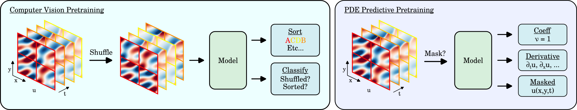
Figure 1: An illustration of pretraining strategies adapted from computer vision (CV) and predicting PDE characteristics. Left: CV methods can be described by different shuffling mechanisms and losses. Binary pretraining only classifies if a sequence is shuffled or not, while TimeSort, SpaceSort and Jigsaw sort sequences shuffled in various ways, either along the spatial, temporal, or combined dimensions. Right: PDE data has inherent structure that can be leveraged to predict underlying characteristics. Coefficients of the PDE can be regressed, as well as its spatial and temporal derivatives. Additionally, inputs can be masked to regress the solution field $u$ and learn underlying dynamics.

3 Methods

3.1 Data Augmentations

Following the prevalence of data augmentation in the broader deep learning community (Chen et al., 2020; Perez & Wang, 2017), we consider the use of data augmentations adapted to the PDE domain.

3.1.1 Lie Point Symmetry Data Augmentations

We consider a recent body of work proposing Lie Point Symmetry Data Augmentations (Brandstetter et al., 2022; Mialon et al., 2023), a set of PDE-specific data augmentations that preserve the underlying dynamics. Mathematically, given a PDE, one can derive a set of transformations $\{g_{1},g_{2},...,g_{n}\}$, each with a parameter $\{\epsilon_{1},\epsilon_{2},...,\epsilon_{n}\}$ that can be randomly sampled to modulate the strength of the transformation. Since some PDEs may exhibit more Lie symmetries than others, we consider only shifting the PDE solution in space (Shift), which is valid for all PDEs considered, to ensure a fair comparison between datasets. For further details on mathematical theory and its implementation in augmenting PDEs, we refer the reader to Mialon et al. (2023) and Olver (1986).

3.1.2 Physics-Agnostic Data Augmentations

In computer vision literature, many successful data augmentations heavily modify inputs (Chen et al., 2020); in particular, cropping and cutting out portions of an image would not respect physics if adapted to the PDE domain. Following this, we investigate the effect of data augmentations that are physics-agnostic, in that they can be applied to any PDE since the augmentation does not preserve the underlying dynamics. Following recent work on denoising neural operator architectures (Hao et al., 2024), we consider adding Gaussian noise during pretraining (Noise). Furthermore, we consider scaling the PDE solution (Scale), an approach similar to a color distortion, in which the PDE solution values are multiplied by a random constant. For certain simple PDEs, scaling can preserve physics, but this is not generally true due to nonlinearities in more complex PDEs. Additional details on hyperparameters and the implementation of data augmentations can be found in Appendix D.4.

3.2 Pretraining Strategies

In this work, we consider using pretraining strategies that are agnostic to the neural operator architecture to ensure compatibility with different applications and future architecture advances, and describe them in Figure 1. This approach is also consistent with the broader computer vision domain, where models are fully shared between pretraining and downstream tasks and can be adapted to different architectures (e.g. CNN, ViT) (Chen et al., 2020; Xie et al., 2022; He et al., 2021). We provide further details on design considerations and the implementation of pretraining strategies in Appendix D.3.

3.2.1 Computer Vision Strategies

Inspired by diverse pretraining strategies to learn image representations, we adapt many pretraining strategies from the computer vision (CV) domain to the PDE domain. In general, these strategies aim to train models through predicting visual attributes or sorting spatio-temporal sequences to learn visual representations without labels.

Firstly, we consider an early work that pretrains a model to verify if a video is in the correct temporal order (Misra et al., 2016). This problem is formulated as a binary classification task in which a shuffled video and the original video are assigned separate labels; within this work, we refer to this as Binary pretraining.

Subsequent work proposed methods that not only verify temporal order, but can also sort temporally shuffled video frames (Lee et al., 2017). This is generally formulated as a $n-$way classification task, where $n$ denotes the number of permutations in which a sequence of frames can be sorted. In the context of physics data, we can opt to shuffle the data spatially or temporally, as such we refer to these two pretraining strategies as TimeSort or SpaceSort. Empirically, SpaceSort does not perform well, so we omit this strategy from our results.

An extension of sorting samples that have been shuffled along a single dimension (e.g., time, space) is to sort samples shuffled across all dimensions. For images, sorting images shuffled along both the $x$ and $y$ axes is implemented by solving jigsaw puzzles, a challenging task that reassembles an image from its shuffled patches (Noroozi & Favaro, 2016). This work has been extended to the video domain by solving spatio-temporal puzzles (Kim et al., 2018). The extension to PDE data requires sorting data that have been partitioned into discrete patches and shuffled along the space and time axes; we refer to this strategy as Jigsaw. One issue is that the number of possible classes scales with the factorial of the number of patches, and many shuffled sequences are not significantly different from each other. To mitigate this, we sample the top $k$ shuffled permutations that maximize the Hamming distance between the shuffled and the original sequence (Noroozi & Favaro, 2016); this ensures that models can see diverse samples during pretraining while limiting the number of classes in the pretraining task.

3.2.2 PDE Predictive Strategies

Within the PDE domain, there are physics-specific characteristics that PDE data exhibit that can be leveraged for pretraining; this is analogous to predicting motion or appearance statistics in vision pretraining tasks (Wang et al., 2019; Yao et al., 2020). One strategy considers the fact that PDE data depends on equation variables and coefficients, and predicting these coefficients from the PDE data could be useful. This is implemented as a regression task, where the coefficient values are regressed from a snapshot of PDE data; we refer to this strategy as Coefficient.

Additionally, PDE data can be described by the derivatives of current physical values. For example, many finite difference schemes rely on spatial and temporal derivatives of the current vector or scalar field to advance the solution in time. Inspired by this, we propose a pretraining strategy that predicts the spatial and temporal derivatives of PDE data. For 2D PDEs, this is implemented as a regression tasks where the fields ($u_{x},u_{y},u_{xx},u_{yy},u_{t}$) are regressed from a solution $u$; we refer to this strategy as Derivative.

Lastly, numerical solutions of PDEs tend to leverage information of local relationships to solve equations. For example, finite difference schemes use information from neighboring nodes to calculate spatial derivatives. Motivated by this, we propose a pretraining strategy that randomly masks data in space and time and uses this incomplete information to reconstruct the full solution. This is implemented by patching the solution in space and time, randomly replacing masked patches with a learnable mask token, and regressing the true solution; we refer to this strategy as Masked.

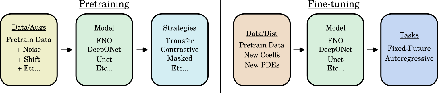
Figure 2: Experimental Setup. During pretraining we consider different data augmentations, model choices, and pretraining tasks and evaluate their downstream performance through fine-tuning on physics prediction tasks. During fine-tuning, we leverage the same pretrained model to improve fixed-future or autoregressive prediction on the same pretraining data distribution, unseen coefficients, or new PDEs. Through this setup we can explore a wide variety of pretraining strategies and augmentations and quantify their effects on different models, PDEs, datasets, and tasks.

3.2.3 Contrastive Strategies

A common strategy for pretraining in computer vision domains is to exploit similarities in the data to align samples in latent space. A proposed strategy to do this for PDEs is Physics Informed Contrastive Learning (PICL), which uses a Generalized Contrastive Loss (Leyva-Vallina et al., 2023) to cluster PDE data based on their coefficients in latent space (Lorsung & Farimani, 2024). Another strategy for self-supervised learning of PDE dynamics is using an encoder to align Lie augmented or physically invariant latent PDE samples (Mialon et al., 2023; Zhang et al., 2023b). Both works require the use of a specific encoder along with the neural operator backbone; to adapt these strategies to our experimental setup we consider directly pretraining the neural operator contrastively with these strategies. However, these methods did not seem to show significant improvements over no pretraining, as such, the results are omitted from the paper.

4 Experiments

To evaluate the effectiveness of the proposed pretraining strategies and data augmentations, we consider a diverse set of experiments and neural operator architectures to train on. In particular, we hope to understand whether different architectures or datasets influence pretraining performance and construct a holistic view of pretraining for diverse PDE applications. We provide an overview of the setup and the different experiments possible in Figure 2.

4.1 Data

We consider predicting physics for the 2D Heat, Advection, Burgers, and incompressible Navier-Stokes equations. These equations describe a diverse range of fluid phenomena and form tasks of varying difficulties. For our experiments, we consider pretraining on a combined set of 2D Heat, Advection, and Burgers data, which contain 9216 data samples (3072 for each equation), as well as fine-tuning on a smaller set of 1024 unseen samples for each PDE. We only pretrain on the Heat, Advection, and Burgers equations since the numerical data for these PDEs are easier to generate, and as a result, transferring pretrained knowledge to more challenging PDEs can be evaluated as a potentially useful method.

4.1.1 Heat, Advection, and Burgers Equations

The 2D Heat, Advection, and Burgers equations are given by:

$$\partial_{t}u-\nu\nabla^{2}u=0,\quad\text{Heat}$$ (1)

$$\partial_{t}u+\mathbf{c}\cdot\nabla u=0,\quad\text{Advection}$$ (2)

$$\partial_{t}u+u(\mathbf{c}\cdot\nabla u)-\nu\nabla^{2}u=0,\quad\text{Burgers}$$ (3)

To ensure a diverse set of physics data, the equation coefficients are randomly sampled according to Zhou & Farimani (2024b). In particular, for the Heat equation, we sample $\nu\in[$2\text{\times}{10}^{-3}$,$2\text{\times}{10}^{-2}$]$, for the Advection equation, we sample $\mathbf{c}=[c_{x},c_{y}]\in[0.1,2.5]^{2}$, and for the Burgers equation, we sample $\nu\in[$7.5\text{\times}{10}^{-3}$,$1.5\text{\times}{10}^{-2}$]$, and $\mathbf{c}=[c_{x},c_{y}]\in[0.5,1.0]^{2}$; we refer to this dataset as in-distribution (In). Since these equations also comprise the pretraining set, we additionally consider a case where the downstream dataset comes from a separate distribution; in this case, we sample $\nu\in[$2\text{\times}{10}^{-2}$,$3\text{\times}{10}^{-2}$]$ for the Heat equation, $\mathbf{c}=[c_{x},c_{y}]\in[2.5,3.0]^{2}$ for the Advection equation, and $\nu\in[$5.0\text{\times}{10}^{-3}$,$7.5\text{\times}{10}^{-3}$]$, and $\mathbf{c}=[c_{x},c_{y}]\in[1.0,1.25]^{2}$ for the Burgers equation. We refer to this dataset as out-of-distribution (Out).

In all cases, periodic boundary conditions are enforced and the solution is solved in a domain $(x,y)=[-1,1]^{2}$ from $t=0$ to $t=2$. Furthermore, initial conditions are randomly from a summation of sine functions; the parameters are uniformly sampled from from $A_{j}\in[-0.5,0.5],\omega_{j}\in[-0.4,0.4],l_{xj}\in\{1,2,3\},l_{yj}\in\{1,2,3\},\phi_{j}\in[0,2\pi)$ while fixing $J=5,L=2$:

$$u(0,x,y)=\sum_{j=1}^{J}A_{j}sin(2\pi l_{xj}x/L+2\pi l_{yj}y/L+\phi_{j})$$ (4)

For additional information on data splits and numerical methods, we refer readers to Appendix D.1.

4.1.2 Incompressible Navier Stokes Equations

The incompressible Navier Stokes equations are considered for fine-tuning pretrained models to predict more challenging physics. To ensure consistency between the pretraining and fine-tuning tasks, we use the vorticity form of the Navier-Stokes equation in order to predict a scalar field following the setup in Li et al. (2021):

$$\partial_{t}\omega+\mathbf{u}\cdot\nabla\omega-\nu\nabla^{2}\omega=f(x,y),\quad\nabla\cdot\mathbf{u}=0,\quad\nabla\times\mathbf{u}=\omega$$ (5)

$$f(x,y)=A(sin(2\pi(x+y))+cos(2\pi(x+y)))$$ (6)

We formulate this problem with periodic boundary conditions, variable viscosity $\nu$, and variable forcing function amplitude $A$. Specifically, the viscosity is sampled uniformly from $\nu\in\{\{1,2,3,4,5,6,7,8,9\}\times 10^{-\{6,7,8,9\}}\}$ and the amplitude is uniformly sampled from $A\in\{\{1,2,3,4,5,6,7,8,9,10\}\times 10^{-3}\}$. The data is generated in a domain $(x,y)=[0,1]^{2}$ and from $t=0$ to $t=7.75$, following the setup from Lorsung et al. (2024); furthermore, the initial conditions $\omega_{0}$ are generated from a Gaussian random field according to Li et al. (2021).

4.2 Neural Operators

To compare different pretraining and data augmentation strategies, we consider their effects on improving the PDE prediction performance of different neural operators. Specifically, we consider the neural operators: Fourier Neural Operator (FNO) (Li et al., 2021), DeepONet (Lu et al., 2021a) and OFormer (Li et al., 2023a). Additionally, we consider the Unet model; while it is not explicitly a neural operator, it is commonly used in literature and has shown good performance (Ronneberger et al., 2015; Gupta & Brandstetter, 2022). These neural operators are first trained using a pretraining strategy before being fine-tuned on a PDE prediction task; this could either be fixed-future prediction to model a static solution or autoregressive prediction to model a time-dependent solution. In all experiments, prediction tasks are formulated using only solution field values and grid information. Additional details on the model hyperparameters and implementation can be found in Appendix D.2.

4.3 Pretraining Strategies

We compare models pretrained with different strategies with a baseline model that has not been pretrained (None) as well as a model trained with the same physics prediction objective on the pretraining dataset, more commonly known as transfer learning (Transfer). Furthermore, we vary the size of the fine-tuning dataset to study the effects of pretraining when given scarce downstream data. The fine-tuning dataset is also varied between data samples that are within the pretraining distribution (In), outside the pretraining distribution with respect to the PDE coefficients (Out), or on samples from an unseen PDE (NS). Lastly, we study the effects of adding data augmentations during pretraining and fine-tuning.

4.4 Data Augmentation

Data augmentation is implemented by doubling the pretraining and fine-tuning data, where each sample has a 50% chance of being augmented. Our noise augmentation adds a small amount of Gaussian noise to each frame independently, while our shift and scale augmentations are applied uniformly to the entire trajectory.

Table 2: Effects of Pretraining for Auto-regressive Prediction: We present comparisons of different pretraining strategies after pretraining on the Heat, Advection, and Burgers equations and fine-tuning in 500 unseen samples.The insights are distilled into two tables, for full results see Appendix A.

(a) The best pretraining strategy varies with model and dataset choice. We compare the highest performing pretraining strategies on autoregressive prediction; although performance varies widely, transfer learning performs well in many settings.

	Best Pretraining Method
Model	Heat	Advection	Burgers	NS
FNO	Derivative	Transfer	PICL	None
DeepONet	PICL	Transfer	Transfer	Transfer
OFormer	Transfer	PICL	Transfer	None
Unet	Transfer	TimeSort	Transfer	Transfer

(b) Different models display different benefits from pretraining. We compare the improvement of the highest performing pretraining strategy to no pretraining. The models show different capacities to be pretrained.

	Improvement w/ Best Strategy
Model	Heat	Advection	Burgers	NS
FNO	14.43%	7.459%	1.430%	0.000%
DeepONet	3.580%	1.852%	15.74%	2.894%
OFormer	38.91%	4.594%	17.12%	0.000%
Unet	29.16%	1.899%	9.706%	1.862%

4.5 Fixed Future and Auto-regressive Prediction

To model physics problems with static solutions, we consider predicting a PDE solution field at a fixed timestep after an initial snapshot of the PDE data. In particular, given the PDE data from $t=1$ to $t=8$, models are trained to predict the PDE solution at $t=32$.

Alternatively, to model physics problems with time-dependent solutions, we consider auto-regressively predicting PDE solutions directly after a current snapshot of PDE data. This is implemented using PDE data on the interval $[t,t+8)$ as an input to predict future PDE solutions on the interval $[t+8,t+16)$. In addition, we use the pushforward trick (Brandstetter et al., 2023) to stabilize training. This introduces model noise during training by first predicting a future time window from ground-truth data and then using this noisy prediction as a model input; importantly, no gradients are propagated through the first forward pass. Additional details on training parameters can be found in D.5.

5 Results

We now systematically benchmark our pretraining and data augmentation strategies, as well as their combination. Presented below are results on our autoregressive task. Fixed-future results are given in appendices A and B and generally show the same trends as our autoregressive results. We use Relative L2 error (Li et al., 2021) for both training and evaluation in all of our experiments.

5.1 Comparison of Pretraining Strategies

We benchmark our proposed PDE pretraining strategies on different neural operators and datasets, and show the condensed results for auto-regressive prediction in Table 2(b). For a detailed comparison, we present results of different PDE pretraining strategies for fixed-future and auto-regressive tasks on all datasets in Appendix A. Additionally, we consider cases where the fine-tuning dataset contains coefficients unseen during pretraining, and present these out-of-distribution results in Appendix A as well.

Table 3: Effects of Data Augmentation for Auto-regressive Prediction: We present comparisons of different pretraining strategies combined with data augmentations after pretraining on the Heat, Advection, and Burgers equations and fine-tuning in 500 unseen samples. The data is distilled into two tables; for full results see Appendix B.

(a) The best pretraining with data augmentation strategy varies with model and dataset. Different models benefit from different augmentations when paired with pretraining strategies. Note: ^p denotes PICL and ^t denotes transfer learning.

	Best Augmentation
Model	Heat	Advection	Burgers	NS
FNO	Shift	Scalet	Nonep	None
DeepONet	Shift	Shiftt	Shiftt	Shiftt
OFormer	Noiset	Nonep	Noiset	Noiset
Unet	Shiftt	Shiftp	Shiftt	Noise

(b) Adding data augmentations consistently improves performance. When choosing the correct combination of pretraining and data augmentation strategies, we find it improves performance during autoregressive prediction compared to baselines.

	Improvement w/ Best Augmentation
Model	Heat	Advection	Burgers	NS
FNO	14.21%	8.287%	1.411%	0.000%
DeepONet	8.745%	1.537%	13.21%	3.761%
OFormer	35.35%	4.426%	16.288%	13.23%
Unet	30.051%	0.735%	10.322%	3.434%

Through these experiments, we find multiple insights. Firstly, we observe that the pretraining performance varies with the choice of model and dataset. Specifically, different models benefit differently from pretraining, as well as based on the predicted PDE and task (i.e. fixed-future vs. auto-regressive). However, transfer learning generally performs well across different tasks, models, and datasets, suggesting that it is a good choice for a pretraining task. This is also reflected in the literature, where previous work generally focuses on transferring knowledge between datasets (Chen et al., 2021; Goswami et al., 2022; Chakraborty et al., 2022; Tripura & Chakraborty, 2023) or pretrain by predicting physics of large datasets (Hao et al., 2024; McCabe et al., 2023; Subramanian et al., 2023). We hypothesize that transfer learning is effective since PDE data is inherently unlabeled; physics prediction uses future timesteps as a label, similar to next-token prediction for GPT models, which is cast as self-supervised learning. When the data is sufficient, using surrogate objectives such as derivatives or sorting sequences may not be as effective as the true objective of fixed-future of auto-regressive prediction. Another observation is that pretraining frameworks are generally dependent on specific architectures; for example, many CV pretraining strategies shuffle patches of data, which can introduce arbitrary discontinuities and high-frequency modes in FNO models, yet are not as challenging for convolutional models such as Unet. Furthermore, pretraining strategies are also dependent on the downstream task; for example, Derivative pretraining works well for auto-regressive prediction but not fixed future prediction, as the solution at a distant timestep is very different from the current derivatives, but the solution at the next timestep is highly dependent on the current derivatives.

Secondly, we observe that directly adapting computer vision methods to the physics domain generally results in poor performance. In many experiments, using a CV pretraining method would often hurt performance compared to not pretraining. This points to a general difference between CV and physics tasks. In the vision domain many downstream tasks are classification-based (i.e. ImageNet, Object Detection, etc.), which results in many pretraining tasks modeled around classification, whereas physics prediction is a high-dimensional regression task. Beyond this, physics predictions not only need to be visually consistent, but also numerically accurate, which can be difficult to learn from a classification task. In fact, using physics-based pretraining methods, such as transferring between prediction tasks, regressing derivatives, or a physics-informed contrastive loss, generally results in better performance.

Lastly, we observe that different models have different capacities for pretraining. For example, the OFormer architecture, which is based on transformers, benefits greatly from pretraining in many scenarios; this could be because transformers lack inductive bias and can model arbitrary relationships. Furthermore, Unet architectures also benefit consistently from pretraining; this is reflected in common convolutional architectures used for pretraining in the CV domain, such as ResNet (He et al., 2015). DeepONet and FNO show smaller improvements with pretraining, suggesting that the architectures are less tailored for pretraining. This is especially true for FNO; we hypothesize that the learned Fourier modes may be very different between tasks, resulting in challenges when transferring weights to new tasks.

5.2 Comparison of Data Augmentations

To study the effects of augmenting data during pretraining and finetuning, we conduct experiments in which data augmentations are added to three pretraining strategies (None, Transfer, PICL). These experiments are run to compare data augmentations to a baseline model that is not pretrained, as well as its effects on the most effective pretraining strategies (i.e. Transfer, PICL). The results are summarized in Table 3(b) for auto-regressive prediction, and the complete results can be found in Appendix B. We find the best augmentation by considering the pretraining strategy and augmentation pairing with the lowest error. To calculate its improvement, this error is compared to a model that is not pretrained.

Table 4: Effects of Downstream Dataset: We compare the effect of pretraining without data augmentation when the downstream dataset is varied—both with the number of samples or the distribution of samples. We find that pretraining benefits more in data-scarce regimes, as well as when the downstream data is similar to the pretraining data.

(a) Pretraining is more beneficial when downstream data is scarce. Improvement is measured by comparing the best pretraining method with no pretraining. We report the average improvement across the Heat, Adv, and Burgers PDEs for a given # of samples and model.

	Best Improvement over None
# Samples	FNO	DeepONet	OFormer	Unet
100	-5.953%	6.755%	47.60%	23.05%
250	4.111%	7.361%	29.60%	18.18%
500	6.875%	6.630%	19.57%	13.59%
1000	2.026%	6.135%	13.27%	2.995%

(b) Pretraining is more beneficial when downstream data is similar to pretraining data. For a given distribution of downstream data, we compare the best pretraining strategy with no pretraining and average across PDEs in the distribution. The models show different generalization capacities.

	Best Improvement over None
Distribution	FNO	DeepONet	OFormer	Unet
In	6.875%	6.630%	19.57%	13.592%
Out	3.920%	-3.383%	34.058%	27.696%
NS	-8.658%	2.899%	-1.608%	1.865%

We find that different models benefit from different augmentations; for example, DeepONet performs well with shifted data, but OFormer performs well with noised data. However, across models, datasets, and downstream tasks, one can generally find a data augmentation that improves performance. This suggests that the most effective pretraining frameworks should incorporate a data augmentation strategy, and indeed the best-performing models considered in this study often make use of data augmentations. Transfer learning performs best in nine of our 12 cases, and shift augmentation performs best in eight of our 12 cases, with their combination performing best in six, suggesting that this combination improves performance best across different data sets and models. We believe that data augmentations can help due to the fact that PDE data remains scarce; numerical simulation is needed for high quality data, and as a result emulating a larger dataset with augmentations is beneficial.

5.3 Scaling Behavior

We compare the effect of pretraining for different numbers of downstream samples in Table 4(b). We measure this effect by finding the best pretraining method for a given model, PDE, and dataset size, then calculating its improvement over no pretraining; after calculating the improvement, we average this metric across the Heat, Advection, and Burgers PDEs for auto-regressive prediction. In general, we observe a trend in which the improvement of pretrained models diminishes as the number of fine-tuning samples increases, which is expected as fine-tuning data approaches the pretraining dataset size. It follows that if the downstream data is abundant, directly training on this would be optimal. Additionally, despite these trends, the relative improvement of different pretraining strategies remains approximately constant between different downstream dataset sizes. An exception to these trends is the FNO model; we hypothesize that learned Fourier modes may be more challenging to fine-tune than other learning mechanisms such as attention matrices or convolutional kernels.

For a detailed comparison of the scaling behavior in individual datasets and models, we refer readers to Appendix C. Empirically, we observe a higher variance between random seeds when using a smaller dataset for fine-tuning. Furthermore, the advection equation can generally be learned with fewer samples and the performance is approximately constant with increasing dataset size. Additionally, different models and pretraining strategies display different scaling behaviors, with some models and pretraining strategies displaying greater increases in performance when fine-tuning to scarce data. This further underscores the importance of proper architecture choices that scale well, such as using transformer-based neural operators. Lastly, scaling behavior is more pronounced in fixed-future experiments; this could be because there is less data in fixed-future experiments due to only predicting a single target per data sample as opposed to predicting multiple targets across a longer auto-regressive rollout.

5.4 Generalization Behavior

We compare the effect of varying the distribution of the downstream dataset on the performance of pretrained models. In particular, we compare fine-tuning to unseen coefficients of the same equation (Out) as well as fine-tuning to an unseen PDE with novel initial conditions and forcing terms (NS); these results are shown in Table 4(b) with 500 fine-tuning samples for auto-regressive prediction. In general, we observe reduced performance when fine-tuning to the Navier-Stokes equations, compared to fine-tuning to samples within the pretraining distribution (In). For certain models, this also holds when fine-tuning to a dataset with unseen coefficients (Out). These generalization behaviors are also approximately consistent between different sample sizes of the fine-tuning dataset. It is important to note that certain pretraining frameworks generalize better than others; for example, Coefficient pretraining largely hurts performance, since the fine-tuning distribution contains different coefficients by construction.

We note that the OFormer and Unet architectures show better performance when fine-tuning to out-of-distribution samples; we hypothesize that this is due to shifts in coefficients causing easier phenomena to model. For example, increasing the diffusivity in the heat equation causes transient effects to be concentrated in a few initial timesteps and sparse behavior for the majority of the rollout. Nevertheless, under certain conditions, pretraining shows generalization to unseen coefficients and PDEs, which is a promising direction.

6 Conclusion

In this work, we compare pretraining strategies for PDEs by examining pretraining frameworks that can be used across different models and datasets. In particular, we consider adapting CV pretraining to the PDE domain through sorting spatio-temporal data to learn underlying dynamics without labels. Furthermore, we derive several PDE characteristics that can be predicted, such as its coefficients, derivatives, or reconstructed input. Lastly, we implement existing contrastive as well as transfer learning strategies to construct a diverse set of pretraining strategies. Notably, these strategies can be applied to any model and PDE problem and are flexible to future advances in architectures or datasets.

Through pretraining with different frameworks and data augmentations, we compare their effects on different PDEs, models, downstream datasets, and fine-tuning tasks. We find that pretraining can be highly dependent on model and dataset choices, but in general transfer learning or physics-based strategies do well. Furthermore, we find that directly adapting pretraining strategies from other domains often fails, motivating the need to design PDE-specific pretraining frameworks. Lastly, we observe that different models have different capacities for pretraining, with transformer and CNN based architectures benefiting the most from pretraining and highlighting the need for architectures that have high capacity and transferability.

To further understand PDE pretraining, we investigate the effect of adding data augmentations and varying the fine-tuning dataset. We find that data augmentations consistently benefit performance, with the shift augmentation showing best performance most often. Combining transfer learning with shift augmentation shows the best performance in the majority of test cases. Additionally, pretraining performance is accentuated when the fine-tuning dataset is scarce or similar to the pretraining distribution. Through establishing a deeper understanding of pretraining for PDEs, we hope that future work can leverage these insights to propose new pretraining strategies and expand on current architectures.

Appendix A Comparison of Pretraining Strategies

A.1 Fixed Future Experiments

Table 5: Models are pretrained on 9216 combined 2D Heat, Advection, and Burgers samples and finetuned on 500 samples for each PDE. Normalized L2 errors ($\times 10^{-1}$) are calculated on 256 validation samples and averaged over five seeds. The lowest errors are given in dark grey, and second lowest errors are given in light grey.

(a) Fixed Future Pretraining Results.

PDE	Model	None	Transfer	Binary	TimeSort	Jigsaw	Coefficient	Derivative	Masked	PICL
Heat	FNO	0.240	0.467	0.813	0.771	0.838	0.387	2.742	0.557	0.182
	DeepONet	0.669	0.246	0.755	0.435	0.598	0.467	0.602	0.483	0.675
	OFormer	0.762	0.275	7.520	8.822	3.450	1.898	0.413	0.531	0.630
	Unet	0.150	0.061	0.378	0.339	0.483	0.234	0.131	0.118	0.145
Adv	FNO	3.533	1.517	7.741	5.427	6.138	6.442	6.205	4.522	3.555
	DeepONet	9.907	9.587	10.006	9.814	9.978	9.875	9.926	9.840	9.952
	OFormer	9.645	5.334	10.006	10.022	10.006	10.010	9.878	9.795	9.206
	Unet	3.962	1.488	5.747	5.568	6.509	9.286	4.909	4.058	3.802
Burgers	FNO	0.704	0.675	1.238	1.120	1.226	1.139	4.461	0.896	0.694
	DeepONet	4.096	3.37	4.758	3.638	3.869	3.776	3.987	3.674	4.195
	OFormer	1.92	1.517	9.318	9.792	5.024	3.610	2.112	1.997	1.994
	Unet	1.027	0.771	1.382	1.174	1.450	1.168	0.918	0.822	0.989
NS	FNO	2.112	2.147	3.500	6.285	3.530	3.874	6.200	2.386	2.232
	DeepONet	5.560	5.226	7.650	5.907	15.208	5.712	5.990	5.610	5.514
	OFormer	3.744	3.801	6.056	6.099	6.099	5.445	4.631	4.670	4.056
	Unet	2.279	1.403	3.261	2.847	3.488	2.493	2.341	2.332	2.262

(b) Out-of-Distribution Fixed Future Pretraining Results.

PDE	Model	None	Transfer	Binary	TimeSort	Jigsaw	Coefficient	Derivative	Masked	PICL
Heat	FNO	7.507	1.619	8.842	8.371	8.957	8.966	13.610	7.219	8.282
	DeepONet	1.008	3.187	1.507	2.570	13.584	2.845	1.846	1.517	2.089
	OFormer	11.142	6.87	12.291	11.981	12.106	11.568	11.862	11.408	11.317
	Unet	5.510	1.034	7.738	6.147	12.880	6.240	4.944	3.968	5.373
Adv	FNO	1.456	1.766	2.406	2.221	2.048	2.013	2.298	2.477	1.407
	DeepONet	9.600	9.558	9.955	9.581	9.654	9.616	9.558	9.555	9.563
	OFormer	8.749	8.23	9.923	9.974	9.750	10.013	7.558	9.187	8.775
	Unet	1.952	2.563	2.746	2.486	2.614	3.162	2.294	1.84	1.802
Burgers	FNO	0.195	0.454	0.685	0.688	0.742	0.307	1.734	0.627	0.19
	DeepONet	0.189	0.122	0.307	0.150	0.240	0.150	0.154	0.144	0.164
	OFormer	0.528	0.163	6.134	6.928	2.400	1.558	0.387	0.448	0.585
	Unet	0.342	0.054	0.333	0.218	0.333	0.147	0.202	0.240	0.340

A.2 Auto-regressive Experiments

Table 6: Models are pretrained on 9216 combined 2D Heat, Advection, and Burgers samples and finetuned on 500 samples for each PDE. Normalized L2 errors ($\times 10^{-1}$) are calculated on 256 validation samples and averaged over five seeds. The lowest errors are given in dark grey, and second lowest errors are given in light grey.

(a) Autoregressive Pretraining Results.

PDE	Model	None	Transfer	Binary	TimeSort	Jigsaw	Coefficient	Derivative	Masked	PICL
Heat	FNO	2.730	5.507	3.888	4.704	3.878	4.838	2.336	3.984	2.584
	DeepONet	2.374	2.429	2.618	2.592	3.046	2.589	2.352	2.32	2.289
	OFormer	4.410	2.694	24.214	11.398	5.498	6.982	3.277	3.274	4.418
	Unet	3.357	2.378	3.286	2.768	2.586	2.406	2.464	2.39	3.019
Adv	FNO	30.890	28.586	30.669	29.888	31.571	29.571	29.875	29.584	30.676
	DeepONet	27.971	27.453	28.058	28.778	28.637	28.307	28.861	28.387	28.016
	OFormer	30.102	30.784	29.677	29.674	29.293	29.299	30.467	30.774	28.719
	Unet	30.640	30.832	30.17	30.058	30.992	31.027	30.579	30.310	30.355
Burgers	FNO	5.104	5.696	6.362	6.640	5.373	6.310	5.168	5.466	5.031
	DeepONet	5.101	4.298	5.706	5.341	5.638	5.702	5.024	5.190	5.167
	OFormer	7.734	6.41	25.731	18.102	10.157	10.026	7.059	7.101	8.293
	Unet	5.440	4.912	6.339	5.763	5.277	5.312	5.280	5.197	5.656
NS	FNO	5.884	6.708	8.626	11.211	7.293	7.276	9.245	6.393	6.086
	DeepONet	6.461	6.274	8.954	6.607	7.118	6.659	6.526	6.587	6.427
	OFormer	10.300	10.466	18.433	16.358	13.065	12.592	10.996	11.750	12.380
	Unet	5.854	5.745	6.461	6.110	6.233	6.011	5.902	5.813	6.285

(b) Out-of-Distribution Autoregressive Pretraining Results.

PDE	Model	None	Transfer	Binary	TimeSort	Jigsaw	Coefficient	Derivative	Masked	PICL
Heat	FNO	25.418	22.835	26.810	41.450	26.346	26.400	25.968	23.83	25.623
	DeepONet	3.062	3.914	3.981	4.208	15.344	5.101	4.291	29.002	3.166
	OFormer	35.888	17.203	33.862	34.864	35.389	33.472	32.803	34.528	32.857
	Unet	16.998	3.965	20.390	17.475	21.936	20.397	13.866	9.126	12.961
Adv	FNO	24.733	23.405	24.166	24.970	24.579	24.426	24.922	24.710	24.730
	DeepONet	26.480	26.179	27.219	26.755	26.832	26.864	26.214	26.288	26.406
	OFormer	25.210	25.344	29.968	28.877	25.325	25.658	25.174	24.269	25.014
	Unet	24.627	24.976	25.053	25.062	24.733	24.688	24.630	24.749	24.558
Burgers	FNO	1.443	3.830	2.688	4.630	2.778	2.646	1.498	3.376	1.424
	DeepONet	1.357	1.408	1.677	1.552	2.150	1.642	1.133	1.629	1.247
	OFormer	3.181	1.706	21.411	8.346	3.942	5.360	2.141	2.198	3.032
	Unet	1.594	1.491	1.930	1.706	1.661	1.517	1.514	1.498	1.804

Appendix B Comparison of Data Augmentations

B.1 Fixed Future Experiments

Table 7: Models are pretrained on 9216 combined 2D Heat, Advection, and Burgers samples and finetuned on 500 samples for each PDE. Each baseline (e.g, None, PICL, Transfer) is followed by its variants with different augmentations (e.g, Noise, P-Shift, T-Scale). Normalized L2 errors ($\times 10^{-1}$) are calculated on 256 validation samples and averaged over five seeds. The lowest errors are given in dark grey, and second lowest errors are given in light grey.

(a) Fixed Future Pretraining Results.

PDE	Model	None	Noise	Shift	Scale	PICL	P-Noise	P-Shift	P-Scale	Transfer	T-Noise	T-Shift	T-Scale
Heat	FNO	0.246	0.183	0.182	0.179	0.182	0.389	0.332	0.169	0.418	0.407	0.445	0.449
	DeepONet	0.670	0.638	0.637	0.661	0.493	0.455	0.457	0.562	0.449	0.407	0.401	0.434
	OFormer	0.763	0.482	0.535	0.650	0.901	0.425	0.467	0.918	0.510	0.340	0.338	0.497
	Unet	0.147	0.163	0.162	0.092	0.145	0.176	0.099	0.163	0.130	0.137	0.133	0.081
Adv	FNO	3.539	3.509	3.549	3.339	3.631	3.722	3.704	3.464	2.017	1.703	1.679	1.695
	DeepONet	9.906	9.807	9.792	9.794	9.713	9.594	9.599	9.737	9.606	9.565	9.557	9.560
	OFormer	9.643	9.508	9.566	8.661	9.690	9.689	9.591	9.559	9.296	8.818	8.716	6.948
	Unet	3.979	3.893	3.906	3.457	3.802	3.320	3.142	3.473	2.401	2.211	2.192	1.930
Burgers	FNO	0.698	0.583	0.584	0.721	0.640	0.643	0.627	0.761	0.645	0.643	0.636	0.831
	DeepONet	4.092	3.840	3.841	3.791	4.101	3.929	3.937	4.018	3.956	3.774	3.770	3.854
	OFormer	1.919	1.612	1.617	1.811	2.408	1.718	1.778	2.158	1.752	1.496	1.506	1.556
	Unet	1.026	0.950	0.988	0.844	0.989	0.722	0.633	0.727	0.952	0.877	0.883	0.812
NS	FNO	2.112	2.122	2.124	2.301	2.232	2.574	2.534	2.335	2.428	2.581	2.602	2.747
	DeepONet	5.560	5.543	5.544	5.552	5.514	5.316	5.320	5.517	5.492	5.313	5.313	5.333
	OFormer	3.744	3.415	3.399	3.569	4.056	3.696	3.694	3.922	3.962	3.629	3.609	3.605
	Unet	2.279	2.247	2.238	2.309	2.262	2.290	2.131	2.318	2.678	2.603	2.573	2.520

(b) Out-of-Distribution Fixed Future Pretraining Results.

PDE	Model	None	Noise	Shift	Scale	PICL	P-Noise	P-Shift	P-Scale	Transfer	T-Noise	T-Shift	T-Scale
Heat	FNO	7.721	7.818	7.805	6.409	8.282	8.670	8.807	7.528	2.431	2.842	2.726	2.806
	DeepONet	1.019	1.056	1.073	1.027	2.089	2.023	2.091	1.228	1.150	1.368	1.384	1.250
	OFormer	11.14	11.58	11.61	11.78	11.32	11.34	11.42	11.51	11.46	11.00	11.18	9.956
	Unet	5.504	5.128	5.203	3.299	5.373	5.070	3.894	3.261	2.491	2.139	2.040	1.783
Adv	FNO	1.457	1.374	1.372	1.305	1.407	1.496	1.487	1.317	1.583	1.601	1.604	1.537
	DeepONet	9.599	9.581	9.585	9.584	9.563	9.513	9.511	9.497	9.523	9.511	9.493	9.492
	OFormer	8.750	8.214	8.251	7.179	8.775	8.833	8.682	8.472	8.997	9.082	8.968	7.807
	Unet	1.955	1.967	2.014	1.623	1.802	1.597	1.582	1.281	2.117	2.137	2.165	1.757
Burgers	FNO	0.214	0.173	0.170	0.148	0.190	0.261	0.265	0.115	0.400	0.425	0.455	0.592
	DeepONet	0.188	0.145	0.146	0.182	0.164	0.126	0.131	0.192	0.126	0.122	0.122	0.122
	OFormer	0.526	0.288	0.326	0.536	0.585	0.289	0.343	0.780	0.362	0.201	0.201	0.368
	Unet	0.341	0.322	0.323	0.313	0.340	0.281	0.216	0.303	0.284	0.229	0.223	0.252

B.2 Auto-regressive Results

Table 8: Models are pretrained on 9216 combined 2D Heat, Advection, and Burgers samples and finetuned on 500 samples for each PDE. Each baseline (e.g, None, PICL, Transfer) is followed by its variants with different augmentations (e.g, Noise, P-Shift, T-Scale). Normalized L2 errors ($\times 10^{-1}$) are calculated on 256 validation samples and averaged over five seeds. The lowest errors are given in dark grey, and second lowest errors are given in light grey.

(a) Autoregressive Pretraining Results.

PDE	Model	None	Noise	Shift	Scale	PICL	P-Noise	P-Shift	P-Scale	Transfer	T-Noise	T-Shift	T-Scale
Heat	FNO	2.731	2.345	2.343	2.405	2.584	2.908	2.830	2.428	4.338	5.398	5.174	5.215
	DeepONet	2.184	2.410	1.993	2.158	2.289	2.120	2.166	2.371	2.347	2.297	2.118	2.378
	OFormer	4.540	3.778	3.854	4.074	4.418	3.658	3.433	4.674	3.190	2.935	3.010	3.218
	Unet	3.301	2.695	2.776	2.387	3.019	2.339	2.349	2.494	2.301	2.340	2.276	2.494
Adv	FNO	30.89	30.88	31.02	30.67	30.68	29.94	30.22	30.11	28.59	28.33	28.65	28.33
	DeepONet	27.98	28.66	28.04	28.01	28.02	28.13	27.840	28.20	28.14	28.04	27.55	27.81
	OFormer	30.05	31.04	30.29	30.31	28.72	28.89	28.84	29.83	30.18	30.23	30.61	30.11
	Unet	29.94	30.56	30.12	30.55	30.36	30.37	29.72	30.64	30.45	30.17	30.64	30.75
Burgers	FNO	5.103	5.127	5.076	5.302	5.031	5.098	5.142	5.311	5.874	6.428	5.988	7.448
	DeepONet	4.884	5.080	4.740	4.577	5.167	4.675	4.666	4.671	4.757	4.484	4.239	4.653
	OFormer	7.754	7.157	7.058	7.519	8.293	7.267	7.044	8.183	6.867	6.491	6.538	6.866
	Unet	5.503	5.334	5.335	5.202	5.656	5.206	5.229	4.980	4.957	4.976	4.935	4.940
NS	FNO	5.884	6.129	6.092	6.032	6.086	6.068	6.078	5.973	6.724	6.874	6.931	7.553
	DeepONet	6.461	6.397	6.404	6.400	6.427	6.393	6.376	6.434	6.310	6.241	6.218	6.276
	OFormer	10.30	8.96	9.011	9.012	12.38	10.60	10.25	11.16	10.78	8.937	9.037	9.183
	Unet	5.854	5.653	5.799	5.851	6.285	5.880	5.883	5.676	5.756	5.686	5.705	5.697

(b) Out-of-Distribution Autoregressive Pretraining Results.

PDE	Model	None	Noise	Shift	Scale	PICL	P-Noise	P-Shift	P-Scale	Transfer	T-Noise	T-Shift	T-Scale
Heat	FNO	25.42	25.48	25.50	23.92	25.62	26.01	25.84	23.69	23.89	25.775	25.82	25.73
	DeepONet	3.267	3.182	3.129	3.197	3.166	3.400	3.232	3.119	3.704	4.027	3.922	3.445
	OFormer	35.67	36.71	36.93	35.54	32.86	32.47	32.53	35.80	25.34	26.61	25.97	23.23
	Unet	16.95	15.37	15.66	11.66	12.96	9.51	10.43	8.279	4.649	4.563	4.687	4.172
Adv	FNO	24.73	25.06	25.05	24.92	24.73	25.22	25.16	24.96	23.69	23.39	23.15	23.316
	DeepONet	26.48	26.03	25.81	25.64	26.41	25.96	25.61	25.64	26.23	25.74	25.98	25.57
	OFormer	25.24	25.27	25.36	25.08	25.01	24.69	24.69	25.35	25.26	25.36	25.23	24.99
	Unet	24.48	24.96	24.70	24.90	24.56	24.93	24.58	24.81	25.14	24.46	24.88	25.09
Burgers	FNO	1.442	1.414	1.443	1.469	1.424	2.121	1.787	1.597	4.185	4.580	4.505	5.062
	DeepONet	1.212	1.335	1.167	1.229	1.247	1.273	1.261	1.291	1.411	1.278	1.467	1.460
	OFormer	3.135	2.624	2.688	2.920	3.032	2.437	2.216	3.404	2.044	1.941	1.908	2.161
	Unet	1.560	1.471	1.543	1.632	1.804	1.529	1.637	1.463	1.377	1.348	1.477	1.447

Appendix C Comparison of Downstream Dataset Size

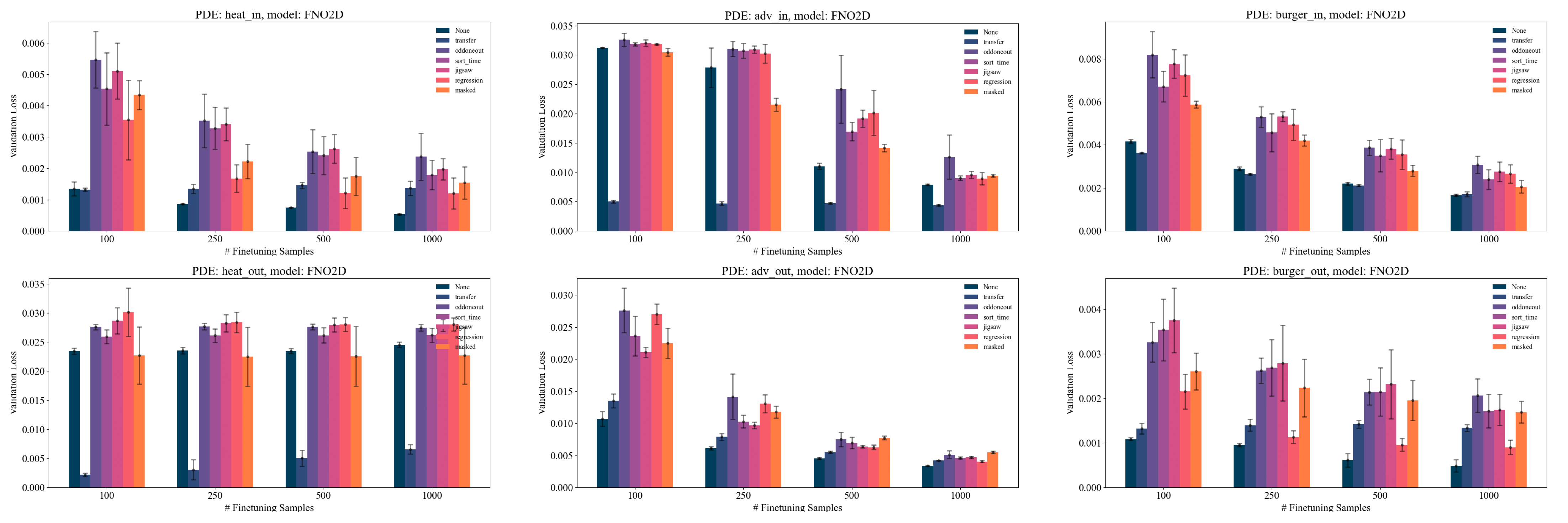
(a) FNO errors across Heat, Advection, and Burgers datasets.

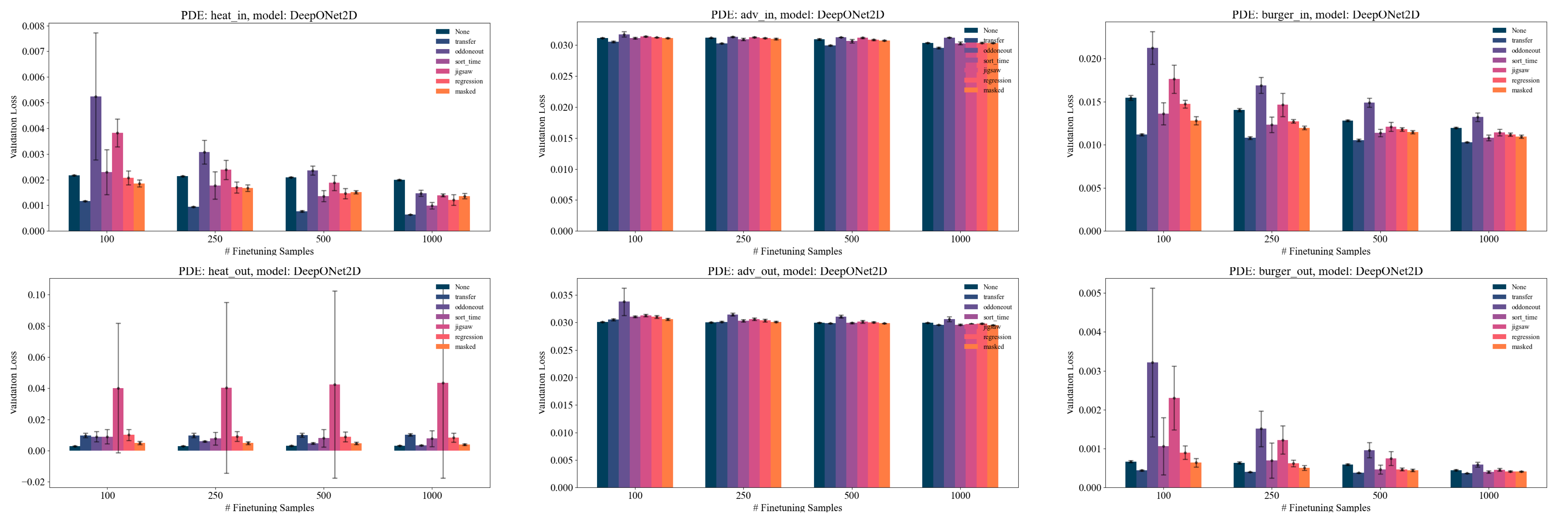
(b) DeepONet errors across Heat, Advection, and Burgers datasets.

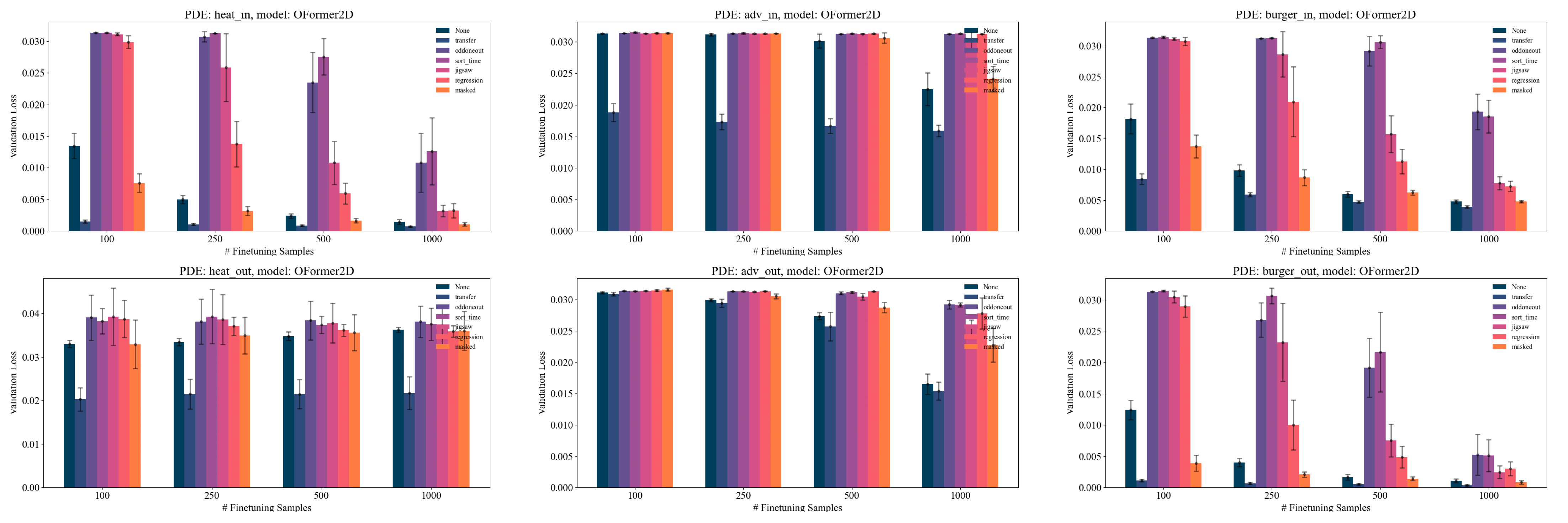
(c) OFormer errors across Heat, Advection, and Burgers datasets.

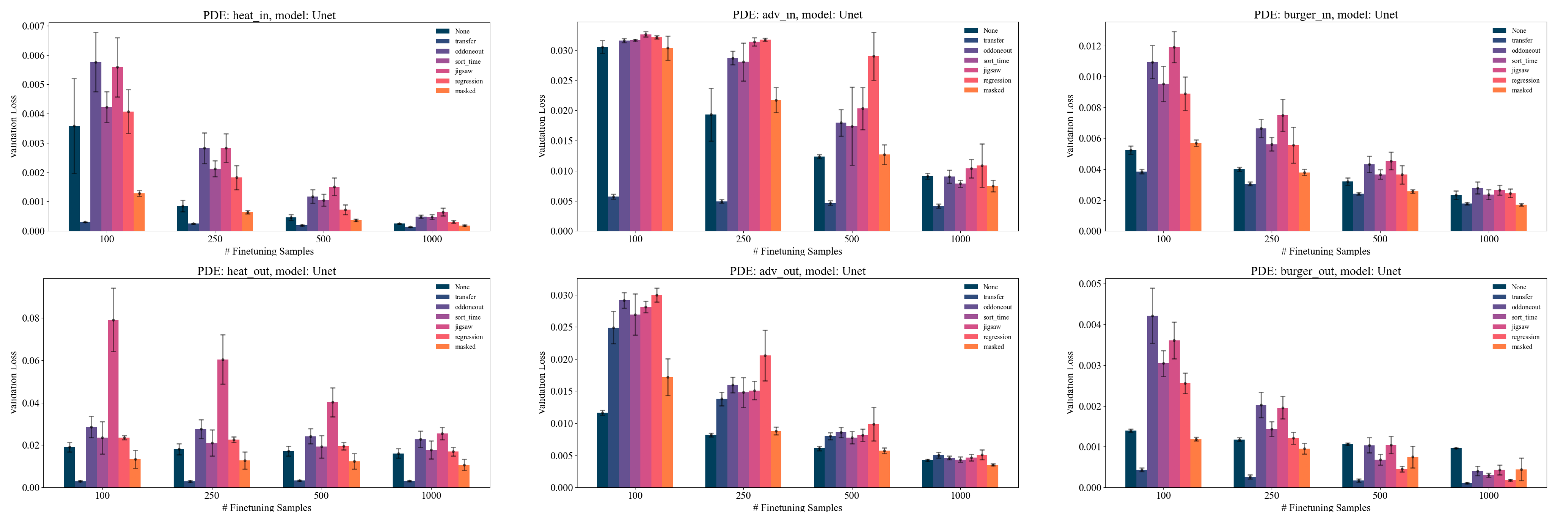
(d) Unet errors across Heat, Advection, and Burgers datasets.

Figure 3: Fixed Future Scaling Behavior: For each model, a specific PDE/distribution is displayed. Within each graph, the performance of various pretraining strategies at different sample sizes is displayed. Validation errors are averaged over 5 seeds, and error bars denote 1 standard deviation. Derivative errors are omitted as outliers.

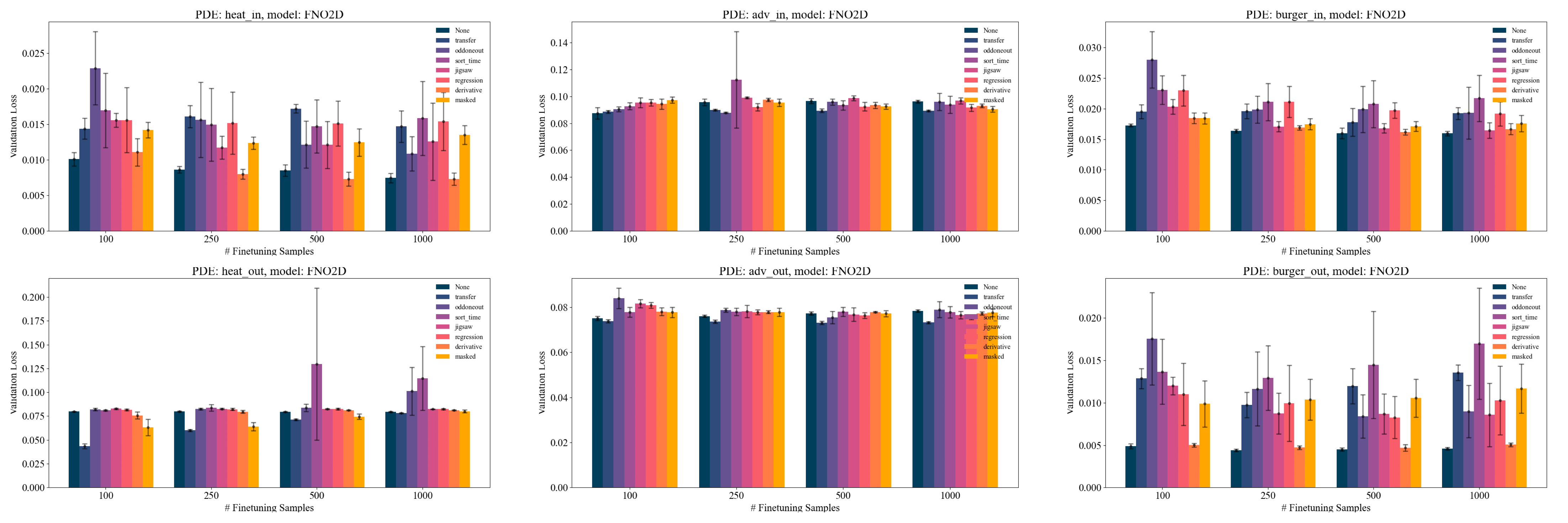
(a) FNO errors across Heat, Advection, and Burgers datasets.

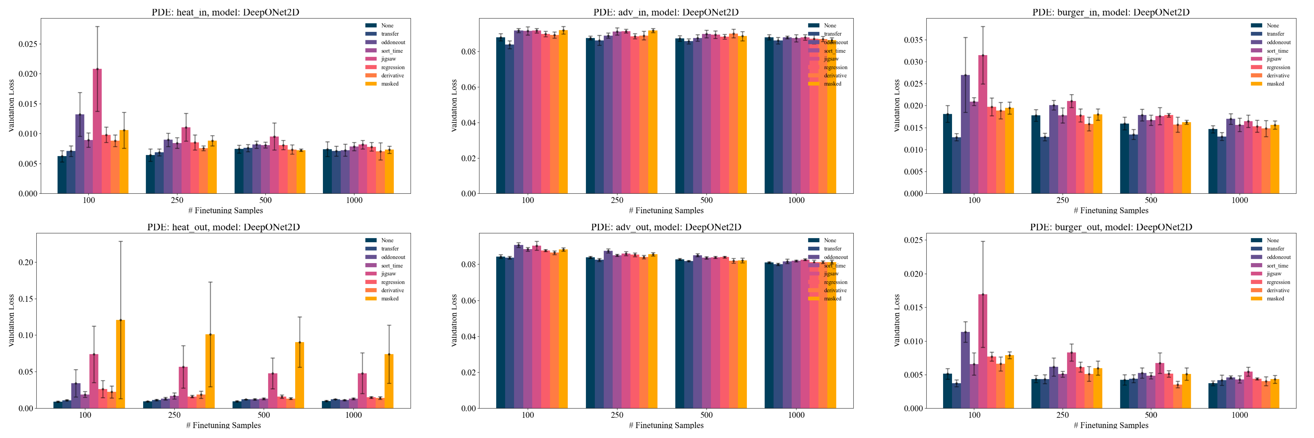
(b) DeepONet errors across Heat, Advection, and Burgers datasets.

(c) OFormer errors across Heat, Advection, and Burgers datasets.

(d) Unet errors across Heat, Advection, and Burgers datasets.

Figure 4: Auto-regressive Scaling Behavior: For each model, a specific PDE/distribution is displayed. Within each graph, the performance of various pretraining strategies at different sample sizes is displayed. Validation errors are averaged over 5 seeds, and error bars denote 1 standard deviation.

Appendix D Implementation Details

D.1 Dataset Details

We generate data according to the equations outlined in 4.1. We provide additional details here:

Pretraining

During pretraining, 9216 total samples are generated, with 3072 samples of the 2D Heat, Advection, and Burgers equations respectively. The samples are generated with a resolution of $(n_{t},n_{x},n_{y})=(32,64,64)$ or $(n_{t},n_{x},n_{y})=(32,32,32)$ on the domain $(x,y)=[-1,1]^{2}$ from $t=0$ to $t=2$; the discretization depends on the downstream resolution of the data. We sample equation coefficients from a defined pretraining distribution. Heat, Advection, and Burgers equation samples are generated with a finite-differences scheme; a first-order central difference is used to discretize the diffusive term, a first-order upwinding scheme is used to discretize the nonlinear convection term, and time is discretized with a forward Euler scheme. In addition, the advection equation is solved with its analytical solution.

Training/Finetuning

During training/fine-tuning, we generate equations using a procedure similar to pretraining and sample coefficients either in the pretraining distribution or from a disjoint distribution to test generalization to unseen coefficients. For fine-tuning on the Navier-Stokes equations, we use a higher resolution of $(n_{t},n_{x},n_{y})=(32,64,64)$, otherwise experiments are run with a resolution of $(n_{t},n_{x},n_{y})=(32,32,32)$. We generate 1024 samples for the Heat, Advection, Burgers, and Navier-Stokes equations to train with. An additional 1024 out-of-distribution samples for the Heat, Advection, and Burgers equations is also generated. Additionally, the Burgers equation, initial conditions are unchanged to evaluate fine-tuning to a reference problem undergoing different dynamics, such as in design optimization problems (Cheng et al., 2024).

Validation

Validation samples are generated similarly to fine-tuning samples, also with equation coefficients sampled from either the pretraining or disjoint distribution. We generate 256 samples for the Heat, Advection, Burgers, and Navier-Stokes equations.

D.2 Model Details

We implement modern FNO and Unet architectures according to Gupta & Brandstetter (2022). Furthermore, we implement DeepONet architectures according to DeepXDE (Lu et al., 2021b), and use the original implementation for OFormer (Li et al., 2023a). The hyperparameters used for the models are described in Table 9(d).

Table 9: Hyperparameters for architectures used.

(a) FNO

Parameter	Value
Modes	4
Width	48
# Layers	4
# Params	300k

(b) DeepONet

Parameter	Value
Branch Size	256
Trunk Size	256
Branch Layers	3
Trunk Layers	3
Activation	SiLU
# Params	250k

(c) OFormer

Parameter	Value
Hidden dim	32
Heads	2
Encoder depth	2
Decoder depth	1
Latent channels	32
# Params	70k

(d) Unet

Parameter	Value
Hidden channels	16
# Blocks	8
Dim Scaling	(1,2,4)
# Params	1M

(a) Embeddings after Binary pretraining. Labels are defined as 0 for shuffled or 1 for original samples.

(b) Embeddings after TimeSort pretraining. Labels are scaled between 0 and 1 for 24 classes.

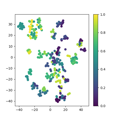
(c) Embeddings after Jigsaw pretraining. Labels are scaled between 0 and 1 for 1000 classes.

Figure 5: t-SNE Embeddings of CV Pretrained Models: We display latent embeddings after pretraining models on Binary, TimeSort. or Jigsaw objectives. We see that models learn to sort/classify sorted samples well and can visualize the relative difficulties of the proposed pretraining strategies.

D.3 Pretraining Details

During pretraining, different strategies require different implementations and hyperparameters. A consideration is that many models need a linear head during pretraining to project model outputs to the classification or regression dimension. Since models will be used for physics prediction, their outputs will be in the shape of the solution field, rather than cross entropy probabilities or regressed values. We use a lightweight CNN projector to downsample and flatten model outputs to the desired dimension. Models are generally trained for 200 epochs with a batch size of 32 using Adam, weight decay, and a OneCycle scheduler for five seeds.

Binary:

Binary pretraining is implemented by shuffling a sample in time and randomly choosing a shuffled or original input with corresponding labels of 0 or 1 to be used for classification. We use a CNN head to project model outputs to a single logit for a binary cross-entropy loss. Within this framework there are a few design decisions. The difficulty of the task can be modulated by the Hamming distance between the shuffled sample and the original sample. For example, if the shuffled sample is not changed much (e.g. only two frames are swapped), the difference between a sorted and shuffled sample is small and thus more challenging to distinguish. We can leverage this to gradually decrease the Hamming distance of shuffled samples to incrementally increase the difficulty of the task over pretraining. Empirically, this does not make a large difference during training so we choose to omit this curriculum learning for simplicity.

An additional consideration is the probability of sampling a shuffled or sorted sample. In theory, there are many more shuffled samples than sorted samples (i.e. more labels with 0 vs. 1); therefore, it may be beneficial to sample more shuffled samples and use a weighted binary cross-entropy loss. In practice this does not significantly affect training, so we uniformly sample sorted or shuffled samples. A final consideration is that PDE solutions generally do not exhibit large changes in time, therefore, we patchify the time dimension when shuffling to create larger changes in shuffled patches. In general, models are able to learn to distinguish between shuffled and original inputs very well, and we display t-SNE embeddings of a pretrained FNO model on a validation set of shuffled and unshuffled samples in Figure 5(a).

TimeSort/SpaceSort:

Sorting along a single dimension is implemented by patchifying the solution field along the desired dimension and shuffling these patches. This is done to create more distinct differences in the shuffled solution, with the patch size controlling the number of permutations of the shuffled sequence. The permutation number affects the difficulty of the sorting task, with large permutation numbers being more difficult since each permutation represents a different class. To mitigate this, we set the patch size to ensure a sequence length of 4 when shuffling, resulting in $4!=24$ classes or permutations of the solution field. The CNN projection head is modified accordingly to output 24 logits for a cross-entropy loss. In general, spatial sorting does not work well nor does training converge, so we omit this from the results; aliasing effects or periodic boundary conditions can make some spatially shuffled samples extremely similar or identical to sorted samples. However, temporal sorting tends to work well, and we display t-SNE embeddings of a pretrained FNO model on a validation set of temporally shuffled samples in Figure 5(b).

Jigsaw:

Jigsaw is implemented similarly to other sorting frameworks, however due to sorting along multiple axes the number of possible shuffled sequences quickly increases. We mitigate this by using spatial and temporal patches to ensure a sequence length of 8 when shuffled, resulting in $8!=40320$ possible permutations. This is still a large number of classes for a task, therefore we deterministically choose 1000 samples with the largest Hamming distance between the shuffled sequence and original sequence. Contrary to the binary case, shuffled samples with larger Hamming distances are more challenging due to needing to sort more patches The CNN projection head is modified accordingly to output 1000 logits for a cross-entropy loss. In general, jigsaw sorting tends to be more challenging, however, models can still display reasonable performance; we display t-SNE embeddings of a pretrained FNO model on a validation set of jigsaw shuffled samples in Figure 5(c).

Coefficient:

Coefficient regression is implemented by extracting coefficient values from the PDE metadata. The CNN projection head is then modified to output the corresponding number of logits for an MSE loss.

Derivative:

We generate labels for derivative regression through taking spatial and time derivatives $\{u_{t},u_{x},u_{y},u_{xx},u_{yy}\}$ of the PDE solution field using FinDiff (Baer, 2018). This introduces an additional design consideration as the label has more values than the input. We modify the CNN projection head to upsample model outputs after convolution to the desired dimension and apply an MSE loss.

Masked:

Masked inputs are generated by splitting inputs into spatial and temporal patches, and selecting a random subset of these to be masked. In our experiments, we choose to mask 75% of patches. Masked patches are replaced with a learnable mask token, and the full input is passed to the model to reconstruct the original solution field. Since the output shape is the same as the downstream target, a projection head is not strictly needed, but we still include a CNN projection head and apply an MSE loss. This follows previous work; models learn transferable latent features by abstracting reconstruction-specific behavior to a decoder (Chen et al., 2020; He et al., 2021).

PICL:

PICL uses the Generalized Contrastive Loss function (Leyva-Vallina et al., 2023) given in equation 7:

$$\mathcal{L}_{GCL}(u_{i},u_{j})=\frac{\psi_{i,j}}{2}d_{physics}(u_{i},u_{j})^{2}+\frac{1-\psi_{i,j}}{2}\text{max}(\tau-d_{physics}(u_{i},u_{j}),0)^{2}$$ (7)

When working with multiple data sets simultaneously, a vector of operator coefficients is constructed as $\theta$. The similarity between systems is given by magnitude-aware cosine similarity: $\psi_{i,j}\left(\theta_{i},\theta_{j}\right)=\frac{\sqrt{\left|\theta_{i}\cdot\theta_{j}\right|}}{\text{max}\left(\left\lVert\theta_{i}\right\rVert,\left\lVert\theta_{j}\right\rVert\right)}$. The distance between samples is calculated in two parts for a given time $t$: $d_{system}(u_{i},u_{j})=u_{i}^{t+1}-u_{j}^{t}$, and $d_{update}=F(G_{\Theta}(u_{i}))-G_{\Theta}(u_{j})$, where $G_{\Theta}$ is our parameterized model, and $F(\cdot)$ is our numerical update. $d_{update}$ is anchored to $d_{system}$ to account for mode collapse, giving us the loss function: $d_{physics}(u_{i},u_{j})=\left\lVert d_{system}(u_{i},u_{j})-d_{update}(u_{i},u_{j})\right\rVert^{2}$. $\tau$ is a hyperparameter that defines a margin, above which samples are considered to be from different classes. For pretraining, we construct the operator coefficient vector as $\theta=\left[\left\lVert\mathbf{c}_{Burgers}\right\rVert,\nu,\left\lVert\mathbf{c}_{Advection}\right\rVert\right]$

D.4 Data Augmentation Details

We implement three data augmentations to evaluate their effects on model performance: noise, shift, and scale.

Noise

Gaussian noise is added to data samples and targets through sampling a Gaussian at zero mean and a prescribed variance: $X_{noise}=X+\sigma^{2}\mathcal{N}(0,I)$. Empirically, we set the variance to $10^{-7}$; when noise levels are too high, model performance can significantly deteriorate.

Shift

Using the Fourier shift theorem, samples can be shifted in space and resampled in the spectral domain (Brandstetter et al., 2022). Shifting PDE solutions in space preserves physics, since the PDEs considered in this work are invariant across space. Mathematically, this can be verified by deriving or looking up the Lie groups for the 2D Advection, Heat, and Burgers equations, for which there are many, and noting that the solutions can be shifted along the X or Y axes (Ibragimov, 1993). We uniformly sample the magnitude of the shift between $[-0.5,0.5]$.

Scale

Scaling PDE solutions respects physics for the Heat and Advection equations, but not the Burgers equation. However, we still choose to include this augmentation to evaluate the effect of physically inconsistent augmentations; in practice, scaling PDE solutions still improves model performance. The implementation is done by multiplying PDE solutions by a constant, which we uniformly sample between $[-0.5,0.5]$.

D.5 Fine-tuning Details

During fine-tuning, models trained until convergence for fixed-future or auto-regressive prediction and repeated for five seeds. In fixed-future prediction, models are given the solution field at $t=[0,8)$ and the target is at $t=32$. For auto-regressive prediction, models are given the solution field at $t=[0,8)$ and the target is at $t=[8,16)$. After this prediction, the models use their own output to predict the next step $t=[16,24)$ until the time horizon of $t=32$. To stabilize auto-regressive rollout, we implement temporal bundling and the pushforward trick (Brandstetter et al., 2023). Losses are calculated using a relative L2 norm (Li et al., 2021); validation losses are averaged across batch size and accumulated over timesteps or, in the case of fixed-future prediction, at only one timestep. For experiments with different fine-tuning sample sizes, samples are randomly chosen from 1024 possible samples to reach the desired number of samples for each seed. We use an Adam optimizer with weight decay and a CosineAnnealing scheduler. All experiments are run on a NVIDIA GeForce RTX 2080Ti GPU.

References

- Baer (2018) M. Baer. findiff software package, 2018. URL https://github.com/maroba/findiff. https://github.com/maroba/findiff.
- Bardes et al. (2022) Adrien Bardes, Jean Ponce, and Yann LeCun. VICReg: Variance-invariance-covariance regularization for self-supervised learning. In International Conference on Learning Representations, 2022. URL https://openreview.net/forum?id=xm6YD62D1Ub.
- Brandstetter et al. (2022) Johannes Brandstetter, Max Welling, and Daniel E. Worrall. Lie Point Symmetry Data Augmentation for Neural PDE Solvers, May 2022. URL http://arxiv.org/abs/2202.07643. arXiv:2202.07643 [cs].
- Brandstetter et al. (2023) Johannes Brandstetter, Daniel Worrall, and Max Welling. Message passing neural pde solvers, 2023.
- Brown et al. (2020) Tom B. Brown, Benjamin Mann, Nick Ryder, Melanie Subbiah, Jared Kaplan, Prafulla Dhariwal, Arvind Neelakantan, Pranav Shyam, Girish Sastry, Amanda Askell, Sandhini Agarwal, Ariel Herbert-Voss, Gretchen Krueger, Tom Henighan, Rewon Child, Aditya Ramesh, Daniel M. Ziegler, Jeffrey Wu, Clemens Winter, Christopher Hesse, Mark Chen, Eric Sigler, Mateusz Litwin, Scott Gray, Benjamin Chess, Jack Clark, Christopher Berner, Sam McCandlish, Alec Radford, Ilya Sutskever, and Dario Amodei. Language models are few-shot learners, 2020.
- Cao et al. (2023) Zhonglin Cao, Rishikesh Magar, Yuyang Wang, and Amir Barati Farimani. Moformer: Self-supervised transformer model for metal–organic framework property prediction. Journal of the American Chemical Society, 145(5):2958–2967, 2023. doi: 10.1021/jacs.2c11420. URL https://doi.org/10.1021/jacs.2c11420. PMID: 36706365.
- Chakraborty et al. (2022) Ayan Chakraborty, Cosmin Anitescu, Xiaoying Zhuang, and Timon Rabczuk. Domain adaptation based transfer learning approach for solving PDEs on complex geometries. Engineering with Computers, 38(5):4569–4588, October 2022. ISSN 1435-5663. doi: 10.1007/s00366-022-01661-2. URL https://doi.org/10.1007/s00366-022-01661-2.
- Chen et al. (2023) Fei-Long Chen, Du-Zhen Zhang, Ming-Lun Han, Xiu-Yi Chen, Jing Shi, Shuang Xu, and Bo Xu. Vlp: A survey on vision-language pre-training. Machine Intelligence Research, 20(1):38–56, Feb 2023. ISSN 2731-5398. doi: 10.1007/s11633-022-1369-5. URL https://doi.org/10.1007/s11633-022-1369-5.
- Chen et al. (2020) Ting Chen, Simon Kornblith, Mohammad Norouzi, and Geoffrey E. Hinton. A simple framework for contrastive learning of visual representations. CoRR, abs/2002.05709, 2020. URL https://arxiv.org/abs/2002.05709.
- Chen et al. (2024) Wuyang Chen, Jialin Song, Pu Ren, Shashank Subramanian, Dmitriy Morozov, and Michael W. Mahoney. Data-efficient operator learning via unsupervised pretraining and in-context learning, 2024.
- Chen et al. (2021) Xinhai Chen, Chunye Gong, Qian Wan, Liang Deng, Yunbo Wan, Yang Liu, Bo Chen, and Jie Liu. Transfer learning for deep neural network-based partial differential equations solving. Advances in Aerodynamics, 3(1):36, December 2021. ISSN 2524-6992. doi: 10.1186/s42774-021-00094-7. URL https://doi.org/10.1186/s42774-021-00094-7.
- Cheng et al. (2024) Ze Cheng, Zhongkai Hao, Xiaoqiang Wang, Jianing Huang, Youjia Wu, Xudan Liu, Yiru Zhao, Songming Liu, and Hang Su. Reference neural operators: Learning the smooth dependence of solutions of pdes on geometric deformations, 2024.
- Devlin et al. (2019) Jacob Devlin, Ming-Wei Chang, Kenton Lee, and Kristina Toutanova. Bert: Pre-training of deep bidirectional transformers for language understanding, 2019.
- Dong et al. (2023) Qingxiu Dong, Lei Li, Damai Dai, Ce Zheng, Zhiyong Wu, Baobao Chang, Xu Sun, Jingjing Xu, Lei Li, and Zhifang Sui. A survey on in-context learning, 2023.
- Finn et al. (2017) Chelsea Finn, Pieter Abbeel, and Sergey Levine. Model-agnostic meta-learning for fast adaptation of deep networks, 2017.
- Goswami et al. (2022) Somdatta Goswami, Katiana Kontolati, Michael D. Shields, and George Em Karniadakis. Deep transfer operator learning for partial differential equations under conditional shift. Nature Machine Intelligence, 4(12):1155–1164, December 2022. ISSN 2522-5839. doi: 10.1038/s42256-022-00569-2. URL https://www.nature.com/articles/s42256-022-00569-2. Number: 12 Publisher: Nature Publishing Group.
- Gupta & Brandstetter (2022) Jayesh K. Gupta and Johannes Brandstetter. Towards Multi-spatiotemporal-scale Generalized PDE Modeling, November 2022. URL http://arxiv.org/abs/2209.15616. arXiv:2209.15616 [cs].
- Hang et al. (2024) Zhou Hang, Yuezhou Ma, Haixu Wu, Haowen Wang, and Mingsheng Long. Unisolver: Pde-conditional transformers are universal pde solvers, 2024.
- Hao et al. (2024) Zhongkai Hao, Chang Su, Songming Liu, Julius Berner, Chengyang Ying, Hang Su, Anima Anandkumar, Jian Song, and Jun Zhu. Dpot: Auto-regressive denoising operator transformer for large-scale pde pre-training, 2024.
- He et al. (2015) Kaiming He, Xiangyu Zhang, Shaoqing Ren, and Jian Sun. Deep residual learning for image recognition, 2015.
- He et al. (2021) Kaiming He, Xinlei Chen, Saining Xie, Yanghao Li, Piotr Dollár, and Ross Girshick. Masked autoencoders are scalable vision learners, 2021.
- Hemmasian & Barati Farimani (2023) AmirPouya Hemmasian and Amir Barati Farimani. Reduced-order modeling of fluid flows with transformers. Physics of Fluids, 35(5):057126, 05 2023. ISSN 1070-6631. doi: 10.1063/5.0151515. URL https://doi.org/10.1063/5.0151515.
- Herde et al. (2024) Maximilian Herde, Bogdan Raonić, Tobias Rohner, Roger Käppeli, Roberto Molinaro, Emmanuel de Bézenac, and Siddhartha Mishra. Poseidon: Efficient foundation models for pdes, 2024.
- Hu et al. (2020) Weihua Hu, Bowen Liu, Joseph Gomes, Marinka Zitnik, Percy Liang, Vijay Pande, and Jure Leskovec. Strategies for pre-training graph neural networks, 2020.
- Ibragimov (1993) Nail H. Ibragimov. CRC Handbook of Lie Group Analysis of Differential Equations: Symmetries, Exact Solutions, and Conservation Laws. Number v. 1. Taylor & Francis, 1993. ISBN 9780849344886. URL https://books.google.com/books?id=mpm5Yq1q6T8C.
- Kaplan et al. (2020) Jared Kaplan, Sam McCandlish, Tom Henighan, Tom B. Brown, Benjamin Chess, Rewon Child, Scott Gray, Alec Radford, Jeffrey Wu, and Dario Amodei. Scaling laws for neural language models, 2020.
- Kim et al. (2018) Dahun Kim, Donghyeon Cho, and In So Kweon. Self-supervised video representation learning with space-time cubic puzzles. 11 2018. URL http://arxiv.org/abs/1811.09795.
- Kirchmeyer et al. (2022) Matthieu Kirchmeyer, Yuan Yin, Jérémie Donà, Nicolas Baskiotis, Alain Rakotomamonjy, and Patrick Gallinari. Generalizing to new physical systems via context-informed dynamics model, 2022.
- Lee et al. (2017) Hsin-Ying Lee, Jia-Bin Huang, Maneesh Singh, and Ming-Hsuan Yang. Unsupervised representation learning by sorting sequences. 8 2017. URL http://arxiv.org/abs/1708.01246.
- Leyva-Vallina et al. (2023) María Leyva-Vallina, Nicola Strisciuglio, and Nicolai Petkov. Data-efficient large scale place recognition with graded similarity supervision. CVPR, 2023.
- Li et al. (2023a) Zijie Li, Kazem Meidani, and Amir Barati Farimani. Transformer for partial differential equations’ operator learning, 2023a.
- Li et al. (2023b) Zijie Li, Dule Shu, and Amir Barati Farimani. Scalable transformer for pde surrogate modeling, 2023b.
- Li et al. (2024) Zijie Li, Anthony Zhou, Saurabh Patil, and Amir Barati Farimani. Cafa: Global weather forecasting with factorized attention on sphere, 2024.
- Li et al. (2021) Zongyi Li, Nikola Kovachki, Kamyar Azizzadenesheli, Burigede Liu, Kaushik Bhattacharya, Andrew Stuart, and Anima Anandkumar. Fourier neural operator for parametric partial differential equations, 2021.
- Li et al. (2023c) Zongyi Li, Nikola Borislavov Kovachki, Chris Choy, Boyi Li, Jean Kossaifi, Shourya Prakash Otta, Mohammad Amin Nabian, Maximilian Stadler, Christian Hundt, Kamyar Azizzadenesheli, and Anima Anandkumar. Geometry-informed neural operator for large-scale 3d pdes, 2023c.
- Liu et al. (2023) Yuxuan Liu, Zecheng Zhang, and Hayden Schaeffer. Prose: Predicting operators and symbolic expressions using multimodal transformers. arXiv preprint arXiv:2309.16816, 2023.
- Lorsung & Farimani (2024) Cooper Lorsung and Amir Barati Farimani. PICL: Physics Informed Contrastive Learning for Partial Differential Equations, January 2024. URL http://arxiv.org/abs/2401.16327. arXiv:2401.16327 [physics].
- Lorsung et al. (2024) Cooper Lorsung, Zijie Li, and Amir Barati Farimani. Physics informed token transformer for solving partial differential equations. Machine Learning: Science and Technology, 5(1):015032, feb 2024. doi: 10.1088/2632-2153/ad27e3. URL https://dx.doi.org/10.1088/2632-2153/ad27e3.
- Lu et al. (2021a) Lu Lu, Pengzhan Jin, Guofei Pang, Zhongqiang Zhang, and George Em Karniadakis. Learning nonlinear operators via deeponet based on the universal approximation theorem of operators. Nature Machine Intelligence, 3(3):218–229, March 2021a. ISSN 2522-5839. doi: 10.1038/s42256-021-00302-5. URL http://dx.doi.org/10.1038/s42256-021-00302-5.
- Lu et al. (2021b) Lu Lu, Xuhui Meng, Zhiping Mao, and George Em Karniadakis. DeepXDE: A deep learning library for solving differential equations. SIAM Review, 63(1):208–228, 2021b. doi: 10.1137/19M1274067.
- Lu et al. (2022) Lu Lu, Xuhui Meng, Shengze Cai, Zhiping Mao, Somdatta Goswami, Zhongqiang Zhang, and George Em Karniadakis. A comprehensive and fair comparison of two neural operators (with practical extensions) based on fair data. Computer Methods in Applied Mechanics and Engineering, 393:114778, April 2022. ISSN 0045-7825. doi: 10.1016/j.cma.2022.114778. URL http://dx.doi.org/10.1016/j.cma.2022.114778.
- McCabe et al. (2023) Michael McCabe, Bruno Régaldo-Saint Blancard, Liam Holden Parker, Ruben Ohana, Miles Cranmer, Alberto Bietti, Michael Eickenberg, Siavash Golkar, Geraud Krawezik, Francois Lanusse, Mariel Pettee, Tiberiu Tesileanu, Kyunghyun Cho, and Shirley Ho. Multiple Physics Pretraining for Physical Surrogate Models, October 2023. URL http://arxiv.org/abs/2310.02994. arXiv:2310.02994 [cs, stat].
- Meidani et al. (2024) Kazem Meidani, Parshin Shojaee, Chandan K. Reddy, and Amir Barati Farimani. Snip: Bridging mathematical symbolic and numeric realms with unified pre-training, 2024.
- Mialon et al. (2023) Grégoire Mialon, Quentin Garrido, Hannah Lawrence, Danyal Rehman, Yann LeCun, and Bobak T. Kiani. Self-Supervised Learning with Lie Symmetries for Partial Differential Equations, July 2023. URL http://arxiv.org/abs/2307.05432. arXiv:2307.05432 [cs, math].
- Misra et al. (2016) Ishan Misra, C. Lawrence Zitnick, and Martial Hebert. Shuffle and learn: Unsupervised learning using temporal order verification. 3 2016. URL http://arxiv.org/abs/1603.08561.
- Nguyen et al. (2023) Tung Nguyen, Johannes Brandstetter, Ashish Kapoor, Jayesh K. Gupta, and Aditya Grover. Climax: A foundation model for weather and climate, 2023.
- Noroozi & Favaro (2016) Mehdi Noroozi and Paolo Favaro. Unsupervised learning of visual representations by solving jigsaw puzzles. 3 2016. URL http://arxiv.org/abs/1603.09246.
- Olver (1986) Peter Olver. Applications of Lie Groups to Differential Equations. Springer New York, NY, 1986.
- Perez & Wang (2017) Luis Perez and Jason Wang. The effectiveness of data augmentation in image classification using deep learning, 2017.
- Rahman et al. (2024) Md Ashiqur Rahman, Robert Joseph George, Mogab Elleithy, Daniel Leibovici, Zongyi Li, Boris Bonev, Colin White, Julius Berner, Raymond A. Yeh, Jean Kossaifi, Kamyar Azizzadenesheli, and Anima Anandkumar. Pretraining codomain attention neural operators for solving multiphysics pdes, 2024.
- Ronneberger et al. (2015) Olaf Ronneberger, Philipp Fischer, and Thomas Brox. U-net: Convolutional networks for biomedical image segmentation, 2015.
- Schiappa et al. (2022) Madeline C. Schiappa, Yogesh S. Rawat, and Mubarak Shah. Self-supervised learning for videos: A survey. 6 2022. doi: 10.1145/3577925. URL http://arxiv.org/abs/2207.00419http://dx.doi.org/10.1145/3577925.
- Shen et al. (2024) Junhong Shen, Tanya Marwah, and Ameet Talwalkar. Ups: Efficiently building foundation models for pde solving via cross-modal adaptation, 2024.
- Subramanian et al. (2023) Shashank Subramanian, Peter Harrington, Kurt Keutzer, Wahid Bhimji, Dmitriy Morozov, Michael Mahoney, and Amir Gholami. Towards Foundation Models for Scientific Machine Learning: Characterizing Scaling and Transfer Behavior, May 2023. URL http://arxiv.org/abs/2306.00258. arXiv:2306.00258 [cs, math].
- Takamoto et al. (2023) Makoto Takamoto, Francesco Alesiani, and Mathias Niepert. CAPE: Channel-attention-based PDE parameter embeddings for sciML, 2023. URL https://openreview.net/forum?id=22z1JIM6mwI.
- Tripura & Chakraborty (2023) Tapas Tripura and Souvik Chakraborty. A foundational neural operator that continuously learns without forgetting, October 2023. URL http://arxiv.org/abs/2310.18885. arXiv:2310.18885 [cs].
- Wang et al. (2019) Jiangliu Wang, Jianbo Jiao, Linchao Bao, Shengfeng He, Yunhui Liu, and Wei Liu. Self-supervised spatio-temporal representation learning for videos by predicting motion and appearance statistics. 4 2019. URL http://arxiv.org/abs/1904.03597.
- Wang et al. (2022a) Yuyang Wang, Rishikesh Magar, Chen Liang, and Amir Barati Farimani. Improving molecular contrastive learning via faulty negative mitigation and decomposed fragment contrast. Journal of Chemical Information and Modeling, 62(11):2713–2725, 2022a. doi: 10.1021/acs.jcim.2c00495. URL https://doi.org/10.1021/acs.jcim.2c00495. PMID: 35638560.
- Wang et al. (2022b) Yuyang Wang, Jianren Wang, Zhonglin Cao, and Amir Barati Farimani. Molecular contrastive learning of representations via graph neural networks. Nature Machine Intelligence, 4(3):279–287, Mar 2022b. ISSN 2522-5839. doi: 10.1038/s42256-022-00447-x. URL https://doi.org/10.1038/s42256-022-00447-x.
- Wei et al. (2022) Jason Wei, Yi Tay, Rishi Bommasani, Colin Raffel, Barret Zoph, Sebastian Borgeaud, Dani Yogatama, Maarten Bosma, Denny Zhou, Donald Metzler, Ed H. Chi, Tatsunori Hashimoto, Oriol Vinyals, Percy Liang, Jeff Dean, and William Fedus. Emergent abilities of large language models, 2022.
- Xie et al. (2022) Zhenda Xie, Zheng Zhang, Yue Cao, Yutong Lin, Jianmin Bao, Zhuliang Yao, Qi Dai, and Han Hu. Simmim: A simple framework for masked image modeling, 2022.
- Yang et al. (2023) Liu Yang, Siting Liu, Tingwei Meng, and Stanley J Osher. In-context operator learning with data prompts for differential equation problems. Proceedings of the National Academy of Sciences, 120(39):e2310142120, 2023.
- Yao et al. (2020) Yuan Yao, Chang Liu, Dezhao Luo, Yu Zhou, and Qixiang Ye. Video playback rate perception for self-supervisedspatio-temporal representation learning. 6 2020. URL http://arxiv.org/abs/2006.11476.
- Yin et al. (2021) Yuan Yin, Ibrahim Ayed, Emmanuel de Bézenac, Nicolas Baskiotis, and Patrick Gallinari. Leads: Learning dynamical systems that generalize across environments. 6 2021. URL http://arxiv.org/abs/2106.04546.
- Zbontar et al. (2021) Jure Zbontar, Li Jing, Ishan Misra, Yann LeCun, and Stéphane Deny. Barlow twins: Self-supervised learning via redundancy reduction, 2021.
- Zhang et al. (2023a) Lu Zhang, Huaiqian You, Tian Gao, Mo Yu, Chung-Hao Lee, and Yue Yu. Metano: How to transfer your knowledge on learning hidden physics, 2023a.
- Zhang et al. (2023b) Rui Zhang, Qi Meng, and Zhi-Ming Ma. Deciphering and integrating invariants for neural operator learning with various physical mechanisms. National Science Review, pp. nwad336, December 2023b. ISSN 2095-5138, 2053-714X. doi: 10.1093/nsr/nwad336. URL http://arxiv.org/abs/2311.14361. arXiv:2311.14361 [physics].
- Zhang et al. (2023c) Zezhong Zhang, Feng Bao, Lili Ju, and Guannan Zhang. Transnet: Transferable neural networks for partial differential equations, 2023c.
- Zhou & Farimani (2024a) Anthony Zhou and Amir Barati Farimani. Faultformer: Pretraining transformers for adaptable bearing fault classification. IEEE Access, 12:70719–70728, 2024a. doi: 10.1109/ACCESS.2024.3399670.
- Zhou & Farimani (2024b) Anthony Zhou and Amir Barati Farimani. Masked autoencoders are pde learners, 2024b.