RILe: Reinforced Imitation Learning
Abstract
Reinforcement Learning has achieved significant success in generating complex behavior but often requires extensive reward function engineering. Adversarial variants of Imitation Learning and Inverse Reinforcement Learning offer an alternative by learning policies from expert demonstrations via a discriminator. Employing discriminators increases their data- and computational efficiency over the standard approaches; however, results in sensitivity to imperfections in expert data. We propose RILe, a teacher-student system that achieves both robustness to imperfect data and efficiency. In RILe, the student learns an action policy while the teacher dynamically adjusts a reward function based on the student’s performance and its alignment with expert demonstrations. By tailoring the reward function to both performance of the student and expert similarity, our system reduces dependence on the discriminator and, hence, increases robustness against data imperfections. Experiments show that RILe outperforms existing methods by 2x in settings with limited or noisy expert data.
1 Introduction
Reinforcement Learning (RL) offers a framework for learning behavior by maximizing a reward function. In recent years, deep reinforcement learning has demonstrated remarkable success in replicating complex behaviors, including playing Atari games, chess, and Go [1, 2]. However, designing a reward function is a tedious and challenging task, as predicting the policy outcome from a manually crafted reward function is difficult.
To address this issue, Imitation Learning (IL) leverages expert demonstrations for learning a policy. Since vast amounts of expert data are required to learn expert behaviors accurately, Adversarial Imitation Learning (AIL) approaches are proposed as a data-efficient alternative to IL [3]. AIL employs a discriminator to measure similarity between learned behavior and expert behavior, and rewards the agent in training accordingly. However, the discriminator tends to overfit to the dynamics of the demonstration setting, limiting its ability to generalize to new environments [4]. Furthermore, AIL is vulnerable to noise or imperfections in expert data, as the discriminator rewards the agent to perfectly mimic expert data, including its flaws.
Inverse Reinforcement Learning (IRL) is another approach to alleviate reward engineering. In contrast to IL, which directly learns expert behavior, IRL seeks to infer the underlying reward function that leads to expert behavior. Thus, the reward function and the agent are trained iteratively, with updates to the reward function based on the agent’s behavior. This iterative process renders IRL computationally expensive [5]. Adversarial Inverse Reinforcement Learning (AIRL) [4] addresses this inefficiency by introducing a discriminator that allows for simultaneous learning of the policy and reward function. By implementing a special structure on the discriminator, AIRL can accurately recover the reward function of an expert, thereby improving generalization to environments with dynamics that vary from the demonstration setting, unlike AIL. However, in contrast to IRL, the reward function in AIRL is not learned independently but is directly derived from the output of the discriminator. Like AIL, AIRL suffers from the data-sensitivity issue associated with the discriminator, which limits its performance when expert data is imperfect.
To learn behaviors from imperfect data in a computationally efficient way, we propose Reinforced Imitation Learning (RILe). The primary motivation of RILe is to maintain computational efficiency and scalability through an adversarial framework, while learning a reward function from expert behavior (akin to IRL) as a separate mechanism. Our framework comprises two interacting agents: a student agent that learns a replicating policy and a teacher agent that learns a reward function and guides the student agent during training. For computational efficiency, we employ a discriminator that distinguishes expert data from student roll-outs as the reward function of the teacher. The core idea behind RILe is that the discriminator guides the reward learning process instead of directly guiding the action policy learning. Our contributions over AIL and AIRL are two-fold:
-
1.
We learn the reward function (teacher agent) of the replicating policy (student agent) as an independent function in an adversarial IL/IRL setting. Using RL, the teacher agent learns to provide rewards that maximize the cumulative reward from the discriminator. The resulting reward function can provide meaningful guidance even when the discriminator overfits to noisy expert data, enabling the replicating policy to navigate and overcome sub-optimal states suggested by imperfect expert demonstrations.
-
2.
The learned reward function in RILe adds an extra layer of flexibility to adversarial IL/IRL settings by allowing the teacher to customize rewards according to the developmental stage of the replicating agent, facilitating more accurate imitation of expert behavior (i.e., "online learned reward shaping").
Our experimental evaluation compares RILe to the state-of-the-art methods of AIL and AIRL, specifically GAIL [3] and AIRL [4], across three distinct sets of experiments: (1) imitating noisy expert data in a grid world, (2) imitating motion-capture data in continuous control tasks, and (3) learning to play image-based Atari games with discrete actions. Experimental results reveal that our approach outperforms baselines by 2x, especially when expert data is limited. We further demonstrate that RILe successfully learns expert-like behavior from noisy and misleading expert data, whereas the baseline methods fail to do so.
2 Related Work
We review the literature on learning expert behavior from demonstrations. Commonly, expert demonstrations are sourced either through direct queries to the expert in any observable state or by collecting sample trajectories demonstrated by the expert. We present related work that aligns with the most prevalent approaches of the latter setting, namely Imitation Learning and Inverse Reinforcement Learning. Both IL and IRL form the conceptual foundation of RILe.
Offline reinforcement learning also learns policies from data, which may include expert demonstrations. In contrast to our setting, its main goal is to learn a policy without any online interactions with the environment. We refer the reader to [6] for an overview of offline RL.
Imitation Learning
The earliest work on imitation learning introduced Behavioral Cloning (BC) [7], which aims to learn a policy congruent with expert demonstrations through supervised learning. DAgger [8] proposes the aggregation of expert demonstrations with policy experiences during the training of the policy for improving generalization over expert demonstrations. GAIL introduces and adversarial imitation learning method, where a discriminator aims to understand whether queried behavior stems from a policy or from expert demonstrations, while a generator tries to fool the discriminator by learning a policy that exhibits expert-like behavior [3]. InfoGAIL extends upon GAIL by extracting latent factors from expert behavior and employing them during imitation learning [9]. Deep Q-learning from Demonstrations (DQfD) proposes to first pre-train the learning agent using expert demonstrations, followed by a subsequent policy optimization through interactions with the environment [10]. ValueDice introduces an off-policy imitation learning method using a distribution-matching objective between policy and expert behavior [11].
Although the field of imitation learning has seen advancements, the need for high-quality expert data and data efficacy remain open challenges [5]. Moreover, the limited generalization capability of IL approaches persists [12]. We address these limitations related to IL’s data efficacy and data sensitivity by introducing an intermediary teacher agent that adapts itself based on the current status of the student agent, enabling the teacher to effectively guide the student beyond the space covered by the expert state-action pairs.
Inverse Reinforcement Learning
IRL is introduced in [13] to learn the intrinsic reward function of an expert and acquire the expert policy from it by iteratively optimizing an agents policy and then reward function. Apprenticeship learning builds on IRL and is proposed to represent the reward function as a linear combination of features [14]. Maximum Entropy Inverse Reinforcement Learning explicitly addresses the noise in expert demonstrations to better recover the reward function [15]. Several works extended IRL by incorporating negative demonstrations into the learning process to further improve behavior modeling [16, 17, 18]. Guided Cost Learning uses a neural network to approximate the reward function by using maximum entropy methods across continuous state-action spaces. [19]. AIRL proposes an adversarial reward learning framework to address the scalability issues of classical approaches [4]. IQ-Learn combines expert data with agent experiences to learn both reward and policy with a single Q-function [20]. Additionally, a pipeline is proposed that enables IRL to handle unstructured, real-world data [21]. XIRL introduces cross-embodiment scenarios, opening up a new direction in IRL research [22].
Despite the advancements in IRL, the computational efficacy of the learning process and scalability to complex problems remain open challenges [23]. The main reason for these limitations is the iterative sequential learning framework employed in IRL. We solve this efficacy problem by learning the policy and the reward function, via training a student agent and a teacher agent, in a single joint learning process.
3 Background
3.1 Preliminaries
A standard Markov Decision Process (MDP) is defined by . is the state space that consists of all possible environment states , and is action space that contains all possible environment actions . is the reward function. is the transition dynamics where is defined as an unknown state state transition probability function upon taking action in state . is the initial state distribution, i.e., and is the discount factor. The policy is a mapping from states to actions. In this work, we consider -discounted infinite horizon settings. Following [3], expectation with respect to the policy refers to the expectation when actions are sampled from : , where is sampled from an initial state distribution , is given by and is determined by the unknown transition model as . The unknown reward function generates a reward given a state-action pair . We consider a setting where is parameterized by as [19].
Our work considers an imitation learning problem from expert trajectories, each consisting of states and actions . The set of expert trajectories are sampled from an expert policy , where is the set of all possible policies. We assume that we have access to expert trajectories, all of which have time-steps, .
3.2 Reinforcement Learning (RL)
Reinforcement learning seeks to find an optimal policy that maximizes the discounted cumulative reward given from the reward function . In this work, we incorporate entropy regularization using the -discounted casual entropy function [3, 24]. The RL problem with a parameterized reward function and entropy regularization is defined as
| (1) |
3.3 Inverse Reinforcement Learning (IRL)
Given sample trajectories of an optimal expert policy , inverse reinforcement learning seeks to recover a reward function that maximally rewards behavior that was sampled from the expert policy . In other words, IRL aims to find a reward function that satisfies
| (2) |
When IRL recovers the optimal reward function, would result in a policy that exhibits expert behavior when optimized with reinforcement learning:
Since only the trajectories created by the expert policy are observed, expectations are estimated from the samples in . In other words, IRL seeks to find the reward function in which the expert policy performs better than any other policy, where the expectation of the expert is estimated through samples. With entropy regularization , maximum casual entropy inverse reinforcement learning [15] can be defined as
| (3) |
3.4 Adversarial Imitation Learning (AIL)
In contrast to inverse reinforcement learning, imitation learning aims to directly approximate the expert policy from given expert trajectory samples. It can be formulated as
| (4) |
where is a loss function, that captures the difference between policy and expert data.
GAIL [3] extends imitation learning to an adversarial setting by quantifying the difference between policies of the agent and the expert with a discriminator , parameterized by . The discriminator’s function is to differentiate between expert-generated state-action pairs and non-expert state-action pairs . Its optimization problem is defined as
| (5) |
Using the discriminator, the goal of GAIL is to find the optimal policy that minimizes this difference metric while maximizing an entropy constraint by training the discriminator and the policy at the same time. The optimization problem can be formulated as a zero-sum game between the discriminator and the policy , represented by
| (6) |
In other words, the reward function that is maximized by the policy is defined as a similarity function, expressed as .
4 RILe: Reinforced Imitation Learning
We propose Reinforced Imitation Learning (RILe) to learn the reward function and acquire a policy that emulates expert-like behavior simultaneously in one learning process. Our framework consists of three key components: a student agent, a discriminator, and a teacher agent (Figure 1).
Intuitively, the student agent learns the action policy and the teacher agent learns the reward function. Both agents are trained simultaneously via RL with the help of an adversarial discriminator. The discriminator enables training the policy and reward function in one learning process and permits replicating expert behavior through similarity rather than supervised state action mapping. However, uniquely in RILe, the discriminator guides the reward learning process instead of directly guiding policy learning. This setup enables the teacher agent to learn a reward function separately by continuously adapting to changes in the student’s policy and guiding the student based on the discriminator’s feedback. As a result, the teacher can understand different regions of the state-action space through student’s interactions, effectively guiding it beyond the potentially noisy and imperfect expert state-action pairs.
In the following, we define the components of RILe and explain how they can efficiently learn behavior from imperfect data.
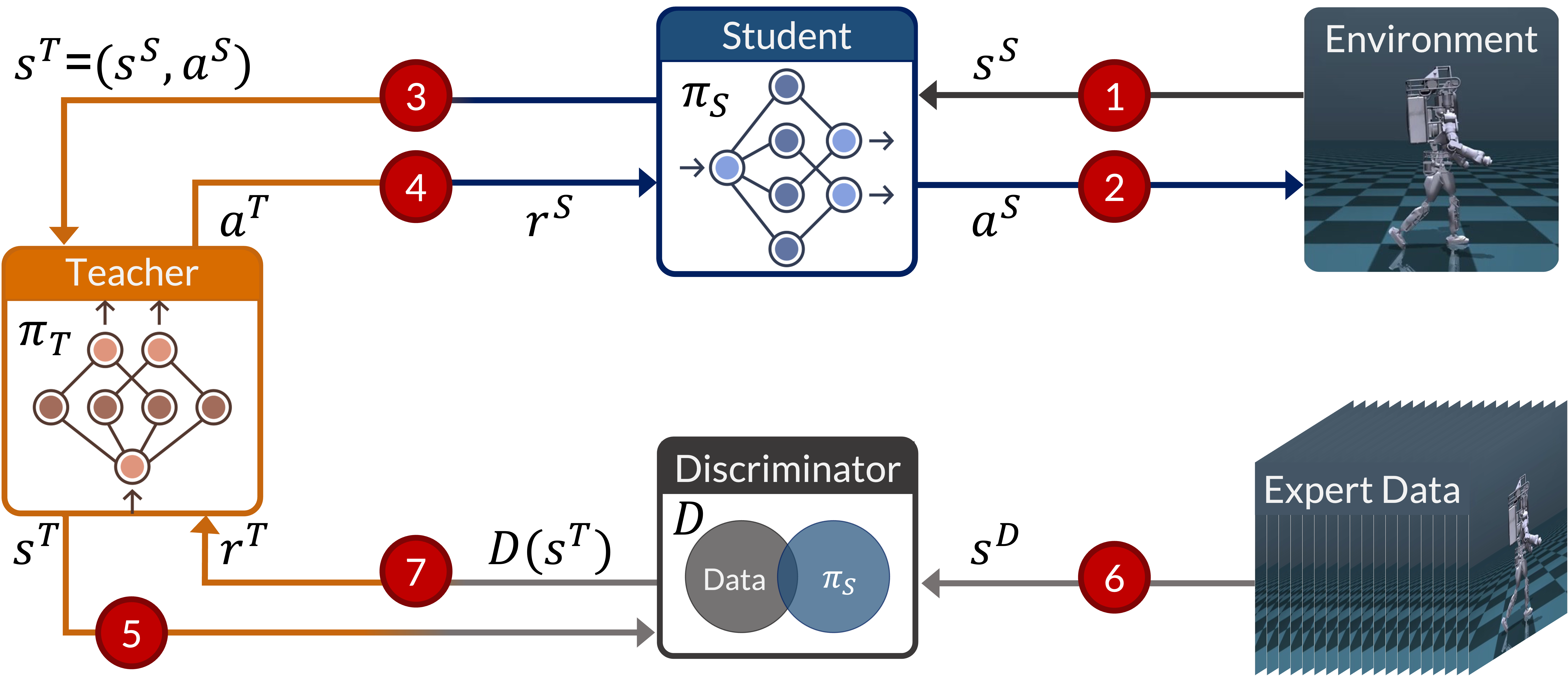
Student Agent
The student agent aims to learn a policy by interacting with an environment in a standard RL setting within an MDP. For each of its actions , the environment returns a new state . However, rather than from a hand-crafted reward function, the student agent receives its reward from the policy of the teacher agent . Therefore, the reward function is represented by the teacher policy. Thus, the student agent is guided by the actions of the teacher agent, i.e., the action of the teacher is the reward of the student: . The optimization problem of the student agent is then defined as
| (7) |
Discriminator
The discriminator differentiates between expert-generated state-action pairs and state-action pairs stemming from the policy of the student . In RILe, the discriminator is defined as a feed-forward deep neural network, parameterized by . Hence, the optimization problem is
| (8) |
To provide effective guidance, the discriminator needs to accurately distinguish whether a given state-action pair originates from the expert distribution or not . The feasibility of this discrimination has been demonstrated by GAIL [3]. The according lemma and proof are presented in the Appendix A.
Teacher Agent
The teacher agent aims to guide the student to approximate expert behavior by operating as its reward mechanism. Since the teacher agent takes the role of a reward function for the student, a new MDP is defined for the teacher agent: , where is the state space that consists all possible state action pairs from the standard MDP, defined in 3.1. is the action space, a mapping from , so the action is a scalar value. is the reward function where and . is the transition dynamics where is defined as the state distribution upon taking action in state . is the initial state distribution.
The teacher agent learns a policy that produces adequate reward signals to guide the student agent, by learning in a standard RL setting, within . Since the state space of is defined over state-action pairs of , the state of the teacher comprises the state-action pair of the student . It generates a scalar action which is given to the student agent as reward , and bounded between -1 to 1. To help the teacher understand how its actions impact the reward it receives, we define the reward function such that it multiplies the discriminator’s output by a sigmoid function dependent on the teacher’s actions. Therefore, the teacher agent’s reward function is defined as , where is the output of the discriminator and is the sigmoid function applied to the teacher’s own actions. Considering only the discriminator’s output in the teacher agent’s reward function would result in a reward independent of the teacher’s actions.
The optimization problem of the teacher can be defined as
| (9) |
RILe
RILe combines the three components defined previously in order to find a student policy that mimics expert behaviors presented in . In RILe, the student policy and the teacher policy can be trained via any single-agent online reinforcement learning method. The training algorithm is given in Appendix C. Overall, the student agent aims to recover the optimal policy defined as
| (10) |
At the same time, the teacher agent aims to recover the optimal policy as
| (11) |
To prove that the student agent can learn expert-like behavior, we need to show that the teacher agent learns to give higher rewards to student experiences that match with the expert state-action pair distribution, as this would enable a student policy to eventually mimic expert behavior.
Lemma 1: Given the discriminator , the teacher agent optimizes its policy via policy gradients to provide rewards that guide the student agent to match expert’s state-action distributions.
Proof for Lemma 1 The assumptions are presented in Appendix A. The expert’s state-action distribution is denoted by . The role of the teacher is to provide a reward signal to the student that encourages the approximation of as closely as possible.
We have as the discriminator, parameterized by , which outputs the likelihood that a given state-action pair originates from the expert, as opposed to the student. The teacher’s policy , parameterized by , aims to maximize the likelihood under the discriminator’s assessment, thus encouraging the student agent to generate state-action pairs drawn from a distribution resembling .
The Value and Q functions of the teacher, conditioned on the rewards provided by the discriminator, are defined in terms of expected cumulative discriminator rewards. The value function for the teacher’s policy parameters at state , simplified from for better readability, is given by:
| (12) |
where . Similarly, the Q-function for taking action in state and then following policy can be written as:
| (13) |
The teacher’s policy optimization is done by maximizing the following clipped surrogate objective function:
| (14) |
where is the advantage function computed as , defined with respect to the teacher’s old policy parameters .
By expressing the advantage using the reward from the discriminator, we explicitly tie the policy gradient updates to the discriminator’s output, emphasizing the shaping of to match :
| (15) |
| (16) |
During each policy update, the objective in Equation 14 is maximized, driving parameter updates to favor actions that elicit higher rewards from the discriminator – effectively the actions that better align with expert behavior:
| (17) |
The update rule in Equation 17, driven by cumulative rewards from the discriminator, incrementally adapts the teacher’s policy to reinforce student behaviors that are indistinguishable from those of the expert according to . The teacher’s policy is guided to facilitate the student’s approximation of , thereby fulfilling its role in the imitation learning process.
5 Experiments
We evaluate the performance of RILe by addressing three key questions. First, can RILe recover a feasible policy when trained to imitate from noisy expert data? To answer this question, we compare RILe’s performance with common imitation learning baselines in a grid world setting where policies are learned from noisy expert data. Second, can RILe use expert-data explicitly to imitate expert behavior? We use MuJoCo [25, 26] to evaluate RILe’s performance when expert data is leaked to the agents. Third, is RILe efficient and scalable to high-dimensional continuous control tasks? We answer this by using LocoMujoco [27] as the benchmark for evaluating RILe’s effectiveness in imitating motion-capture data within continuous robotic control tasks.
Baselines We compared RILe with four baseline methods: Behavioral cloning (BC [7, 28]), adversarial imitation learning (GAIL [3]), adversarial inverse reinforcement learning (AIRL [4]) and inverse reinforcement learning (IQ-Learn [20]).
5.1 Noisy Expert Data
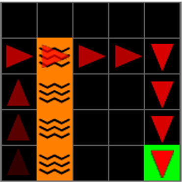
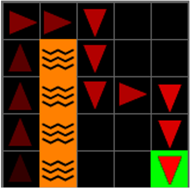
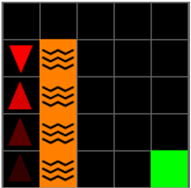
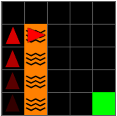
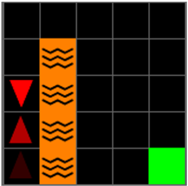
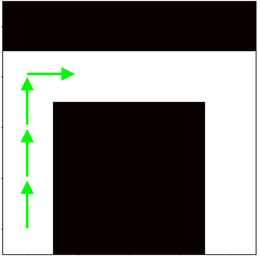
To demonstrate the advantage of using RL to learn the reward function in RILe, as opposed to deriving the reward directly from the discriminator in AIL and AIRL, we designed a 5x5 MiniGrid experiment. The grid consists of 4 lava tiles that immediately kill the agent if it steps in it, representing terminal conditions. The goal condition of the environment is reaching the green tile.
The expert demonstrations are imperfect, depicting an expert that passes through a lava tile without being killed and still reaches the green goal tile. Using this data, we trained the adversarial approaches with a perfect discriminator, which provides a reward of if the visited state-action pair stems from the expert and otherwise. These values were chosen over 1 and 0 because both AIRL and GAIL use the logarithm of the discriminator output to calculate rewards.
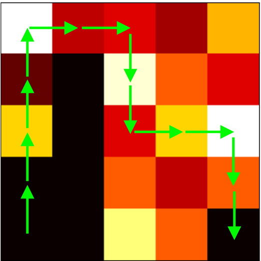
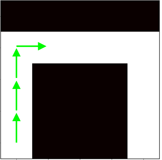
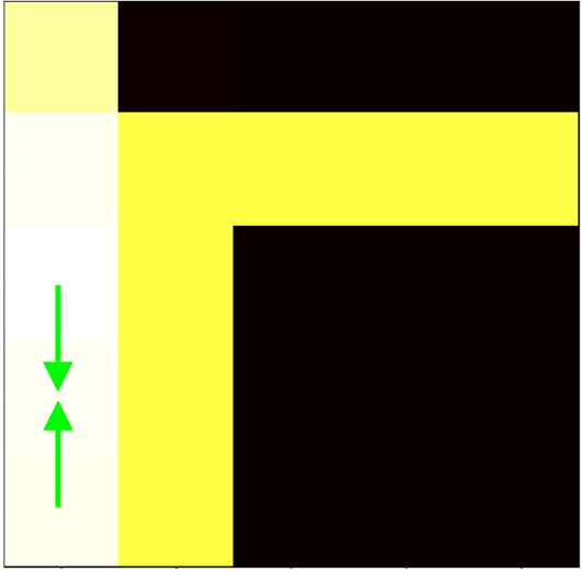
Results are presented in Fig. 2. The value graphs (Fig. 2e-g) are attained by computing the value of each grid cell as for AIRL and GAIL, and for RILe. Fig. 2a shows the expert trajectory.
GAIL (Fig. 2c), AIRL (Fig. 2d) and IQLearn (Fig. 2e) fail to reach the goal, as their agents either become stuck or are directed into lava. In contrast, RILe (Fig. 2d) successfully reaches the goal, demonstrating its ability to navigate around imperfections in expert data. The difference in the value graphs between RILe and the baselines intuitively explains this outcome. In AIL and AIRL (Fig. 2f-g), the optimal paths, defined by the actions most rewarded by their discriminators, follow the noisy expert data perfectly. Similarly, in IQLearn, the agent tries to match expert state-actions as closely as possible, minimizing any deviation from the expert trajectory. In contrast, RILe’s teacher agent, trained using RL, adds an extra degree of freedom in the adversarial IL/IRL setting. By providing rewards that maximize cumulative returns from the discriminator, rather than deriving the reward directly from its output, the value graph (Fig. 2f) can learn to circumvent the lava tile in order to follow the expert trajectory to the goal. Consequently, the optimal path of the student agent can overcome the sub-optimal state suggested by the noisy expert demonstration. Since the student agent is guided by the teacher to also match the expert trajectory, it remains close to this path after passing the lava tiles.
5.2 Expert Data Leakage in Training
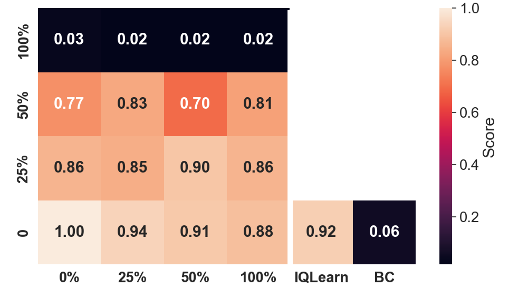
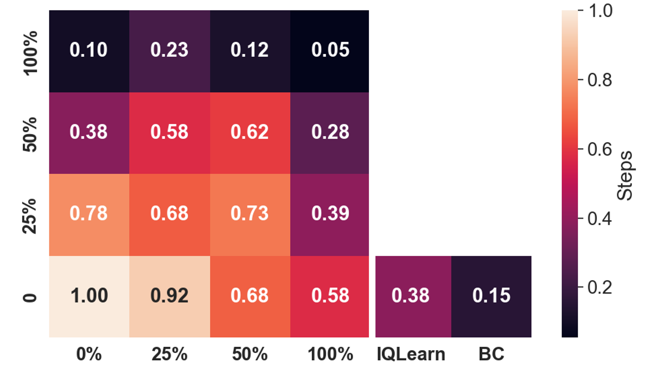
We investigate whether RILe can use expert data explicitly to imitate expert behavior better. Thus, we analyze how the performance and convergence time will be effected when we leak expert data to the replay buffers of both student and teacher agent. For this experiment, we employed MuJoCo’s Humanoid environment [26, 25] and used a single trajectory from the expert data of [20]. The expert data is leaked to agents’ replay buffers with following percentages: . signifies that of the replay buffer’s data is sourced from the expert trajectory, while the remaining originates from the agents’ interactions with the environment. indicates that the agents’ environment interactions are entirely disregarded, with only expert data being used for training.
As shown in Figure 3, leaking expert data to buffers slightly worsened performance but significantly reduced the convergence time. However, when environment interactions were entirely replaced with expert data, the policy’s performance declined substantially. For comparison, results from IQLearn and Behavioral Cloning are also presented, as both methods rely exclusively on expert data for training. Neither method, however, achieved the same level of performance as RILe.
5.3 Motion-Capture Data Imitation for Robotic Continuous Control
In LocoMujoco, the objective is to learn policies that can accurately imitate the collected MoCap data of various robotic tasks. LocoMujoco is challenging due its high dimensionality. The MoCap data only consists of states of the robot, not its actions, which prevents the use of Behavioral Cloning and IQLearn in this analysis, since they both requires to have full expert data with states and actions. It should be noted that LocoMujoco environments do not have terminal or goal conditions.
Results are presented in Table 1 for both test seeds and validation seeds. RILe outperforms baselines especially for new initial conditions introduced by varying seeds.
| Test Seeds | Validation Seeds | ||||||
| RILe | GAIL | AIRL | RILe | GAIL | AIRL | Expert | |
| Atlas Walk | 870.6 | 792.7 | 300.5 | 895.4 | 918.6 | 356 | 1000 |
| Atlas Carry | 850.8 | 669.3 | 256.4 | 889.7 | 974.2 | 271.9 | 1000 |
| Talos Walk | 842.5 | 442.3 | 102.1 | 884.7 | 675.5 | 103.4 | 1000 |
| Talos Carry | 220.1 | 186.3 | 134.2 | 503.3 | 338.5 | 74.1 | 1000 |
| UnitreeH1 Walk | 898.3 | 950.2 | 568.1 | 980.7 | 965.1 | 716.2 | 1000 |
| UnitreeH1 Carry | 788.3 | 634.6 | 130.5 | 850.6 | 637.4 | 140.9 | 1000 |
| Humanoid Walk | 831.3 | 181.4 | 80.1 | 970.3 | 216.2 | 78.2 | 1000 |
6 Discussion
We have demonstrated through our experiments that RILe outperforms baseline models across various settings. While RILe surpasses the state-of-the-art adversarial IL/IRL methods, it also has its limitations. The main challenge is training the policy with a changing reward function, which leads to unstable policy updates for the student agent. To address this issue, we formulate the teacher’s reward by correlating its actions with the output of the discriminator, instead of only relying on the discriminator. However, instability remains a challenge and causes slower learning of the action policy in RILe compared to AIL. Future work should establish bounds for the reward agent updates to enhance the stability of the student agent’s learning process.
Moreover, balancing the learning rates of the discriminator and the policies is challenging, particularly because the discriminator tends to overfit the data quickly. This overfitting makes it difficult for the teacher agent to find a reward for the student that can challenge the discriminator. While adjusting the discriminator’s learning rate on a case-by-case basis helps, future research should focus on a fundamental solution, such as replacing the discriminator with a more robust similarity component.
Uniquely in RILe, the discriminator guides the reward learning process instead of directly guiding policy learning. Therefore, the reward function is learned, not directly derived from the discriminator. This distinction allows RILe to provide meaningful guidance even when the discriminator overfits to noisy expert data. In the LocoMujoco benchmark, where perfect expert data is available, we argue that RILe’s ability to account for the agent’s exploration efforts during training, in addition to its behavioral similarity with the expert, results in a superior generalization capability compared to AIL and AIRL.
References
- [1] V. Mnih, K. Kavukcuoglu, D. Silver, A. Graves, I. Antonoglou, D. Wierstra, and M. Riedmiller, “Playing atari with deep reinforcement learning,” arXiv preprint arXiv:1312.5602, 2013.
- [2] D. Silver, T. Hubert, J. Schrittwieser, I. Antonoglou, M. Lai, A. Guez, M. Lanctot, L. Sifre, D. Kumaran, T. Graepel, et al., “A general reinforcement learning algorithm that masters chess, shogi, and go through self-play,” Science, vol. 362, no. 6419, pp. 1140–1144, 2018.
- [3] J. Ho and S. Ermon, “Generative adversarial imitation learning,” Advances in neural information processing systems, vol. 29, 2016.
- [4] J. Fu, K. Luo, and S. Levine, “Learning robust rewards with adverserial inverse reinforcement learning,” in International Conference on Learning Representations, 2018.
- [5] B. Zheng, S. Verma, J. Zhou, I. W. Tsang, and F. Chen, “Imitation learning: Progress, taxonomies and challenges,” IEEE Transactions on Neural Networks and Learning Systems, no. 99, pp. 1–16, 2022.
- [6] S. Levine, A. Kumar, G. Tucker, and J. Fu, “Offline reinforcement learning: Tutorial, review, and perspectives on open problems,” arXiv preprint arXiv:2005.01643, 2020.
- [7] M. Bain and C. Sammut, “A framework for behavioural cloning.” in Machine Intelligence 15, 1995, pp. 103–129.
- [8] S. Ross, G. Gordon, and D. Bagnell, “A reduction of imitation learning and structured prediction to no-regret online learning,” in Proceedings of the fourteenth international conference on artificial intelligence and statistics. JMLR Workshop and Conference Proceedings, 2011, pp. 627–635.
- [9] Y. Li, J. Song, and S. Ermon, “Infogail: Interpretable imitation learning from visual demonstrations,” Advances in Neural Information Processing Systems, vol. 30, 2017.
- [10] T. Hester, M. Vecerik, O. Pietquin, M. Lanctot, T. Schaul, B. Piot, D. Horgan, J. Quan, A. Sendonaris, I. Osband, et al., “Deep q-learning from demonstrations,” in Proceedings of the AAAI Conference on Artificial Intelligence, vol. 32, no. 1, 2018.
- [11] I. Kostrikov, O. Nachum, and J. Tompson, “Imitation learning via off-policy distribution matching,” in International Conference on Learning Representations, 2020.
- [12] S. Toyer, R. Shah, A. Critch, and S. Russell, “The magical benchmark for robust imitation,” Advances in Neural Information Processing Systems, vol. 33, pp. 18 284–18 295, 2020.
- [13] A. Y. Ng and S. J. Russell, “Algorithms for inverse reinforcement learning,” in Proceedings of the Seventeenth International Conference on Machine Learning, 2000, pp. 663–670.
- [14] P. Abbeel and A. Y. Ng, “Apprenticeship learning via inverse reinforcement learning,” in Proceedings of the twenty-first international conference on Machine learning, 2004, p. 1.
- [15] B. D. Ziebart, A. L. Maas, J. A. Bagnell, A. K. Dey, et al., “Maximum entropy inverse reinforcement learning.” in Proceedings of the AAAI Conference on Artificial Intelligence, vol. 8. Chicago, IL, USA, 2008, pp. 1433–1438.
- [16] K. Lee, S. Choi, and S. Oh, “Inverse reinforcement learning with leveraged gaussian processes,” in 2016 IEEE/RSJ International Conference on Intelligent Robots and Systems (IROS). IEEE, 2016, pp. 3907–3912.
- [17] K. Shiarlis, J. Messias, and S. Whiteson, “Inverse reinforcement learning from failure,” in Proceedings of the 2016 International Conference on Autonomous Agents & Multiagent Systems, 2016, pp. 1060–1068.
- [18] K. Bogert, J. F.-S. Lin, P. Doshi, and D. Kulic, “Expectation-maximization for inverse reinforcement learning with hidden data,” in Proceedings of the 2016 International Conference on Autonomous Agents & Multiagent Systems, 2016, pp. 1034–1042.
- [19] C. Finn, S. Levine, and P. Abbeel, “Guided cost learning: Deep inverse optimal control via policy optimization,” in International conference on machine learning. PMLR, 2016, pp. 49–58.
- [20] D. Garg, S. Chakraborty, C. Cundy, J. Song, and S. Ermon, “Iq-learn: Inverse soft-q learning for imitation,” Advances in Neural Information Processing Systems, vol. 34, pp. 4028–4039, 2021.
- [21] A. S. Chen, S. Nair, and C. Finn, “Learning generalizable robotic reward functions from" in-the-wild" human videos,” in Robotics: Science and Systems, 2021.
- [22] K. Zakka, A. Zeng, P. Florence, J. Tompson, J. Bohg, and D. Dwibedi, “Xirl: Cross-embodiment inverse reinforcement learning,” in Conference on Robot Learning. PMLR, 2022, pp. 537–546.
- [23] S. Arora and P. Doshi, “A survey of inverse reinforcement learning: Challenges, methods and progress,” Artificial Intelligence, vol. 297, p. 103500, 2021.
- [24] M. Bloem and N. Bambos, “Infinite time horizon maximum causal entropy inverse reinforcement learning,” 53rd IEEE Conference on Decision and Control, pp. 4911–4916, 2014. [Online]. Available: https://api.semanticscholar.org/CorpusID:14981371
- [25] G. Brockman, V. Cheung, L. Pettersson, J. Schneider, J. Schulman, J. Tang, and W. Zaremba, “Openai gym,” 2016.
- [26] E. Todorov, T. Erez, and Y. Tassa, “Mujoco: A physics engine for model-based control,” in 2012 IEEE/RSJ international conference on intelligent robots and systems. IEEE, 2012, pp. 5026–5033.
- [27] F. Al-Hafez, G. Zhao, J. Peters, and D. Tateo, “Locomujoco: A comprehensive imitation learning benchmark for locomotion,” in 6th Robot Learning Workshop, NeurIPS, 2023.
- [28] S. Ross and D. Bagnell, “Efficient reductions for imitation learning,” in Proceedings of the thirteenth international conference on artificial intelligence and statistics. JMLR Workshop and Conference Proceedings, 2010, pp. 661–668.
Appendix A Justification of RILe
Assumptions:
-
•
The discriminator loss curve is complex and the discriminator function, , is sufficiently expressive since it is parameterized by a neural network with adequate capacity.
-
•
For the teacher’s and student’s policy functions and , and the Q-functions , each is Lipschitz continuous with respect to its parameters with constants , respectively. This means for all and for any pair of parameter settings
A.1 Lemma 2:
The discriminator , parameterized by will converge to a function that estimates the probability of a state-action pair being generated by the expert policy, when trained on samples generated by both a student policy and an expert policy .
Proof for Lemma 2: The training objective for the discriminator is framed as a binary classification problem over mini-batches from expert demonstrations and student-generated trajectories. The discriminator’s loss function is the binary cross-entropy loss, which for a mini-batch of size is defined as:
| (18) |
where are sampled state-action pairs from the combined replay buffer , with corresponding labels indicating whether the pair is from the expert or the student . The stochastic gradient descent update rule for optimizing is then given by:
| (19) |
where is the learning rate for the discriminator.
Through iterative updates, will converge to , provided the minimization of progresses according to the theoretical foundations of stochastic gradient descent. The convergence relies on the assumption that the student’s policy and the expert policy induce stationary distributions of state-action pairs, such that the discriminator’s data source is consistently representing both policies over time.
By minimizing , we seek such that:
| (20) |
Under typical conditions for convergence in stochastic gradient descent, the convergence to a local minimum or saddle point can be guaranteed. The discriminator’s ability to distinguish between student and expert pairs improves as is minimized, implying that , where is the number of batches.
Appendix B Compute Resources
For the training of RILe and baselines, following computational sources are employed:
-
•
AMD EPYC 7742 64-Core Processor
-
•
1 x Nvidia RTX6000 GPU
-
•
32GB Memory
Appendix C Algorithm
| (21) |
| (22) |
| (23) |