Hierarchical Bayesian Emulation of the Expected Net Present Value Utility Function via a Multi-Model Ensemble Member Decomposition

Abstract

Computer models are widely used to study complex real world physical systems. However, there are major limitations to their direct use including: their complex structure; large numbers of inputs and outputs; and long evaluation times. Bayesian emulators are an effective means of addressing these challenges providing fast and efficient statistical approximation for computer model outputs. It is commonly assumed that computer models behave like a “black-box” function with no knowledge of the output prior to its evaluation. This ensures that emulators are generalisable but potentially limits their accuracy compared with exploiting such knowledge of constrained or structured output behaviour. We assume a “grey-box” computer model and establish a hierarchical emulation framework encompassing structured emulators which exploit known constrained and structured behaviour of constituent computer model outputs. This achieves greater physical interpretability and more accurate emulator predictions. This research is motivated by and applied to the commercially important TNO OLYMPUS Well Control Optimisation Challenge from the petroleum industry. We re-express this as a decision support under uncertainty problem. First, we reduce the computational expense of the analysis by identifying a representative subset of models using an efficient multi-model ensemble subsampling technique. Next we apply our hierarchical emulation methodology to the expected Net Present Value utility function with well control decision parameters as inputs.
Keywords: Computer models; Bayesian emulation; Bayes linear; Known simulator behaviour; Multi-model ensembles; Decision support under uncertainty.

1 Introduction

Mathematical models of complex real world physical systems in the form of numerical codes known as computer models or simulators are prevalent across many scientific disciplines, industry, and government. They are used to: study the dynamics of physical systems; calibrate or history match to observation data; and to guide decision making processes. However, computer models commonly exhibit a complex structure; possess large numbers of inputs and outputs, including spatial-temporal fields; and crucially have a high computational expense of evaluation. In order to address such challenges, a suite of Bayesian uncertainty analysis methodology has been developed for using computer models to perform inferences about real world systems. Of principal importance are Bayesian emulators, also known as surrogate models, which provide fast statistical approximations to (functions of) the computer model outputs for as yet unevaluated parameter settings, along with a corresponding statement of the associated uncertainty. They are typically many orders of magnitude quicker to evaluate than the computer model. Emulators have been successfully employed across a wide range of applications including: climate science [17, 35, 48, 10]; cosmology [41, 42, 21, 25]; epidemiology [2, 3, 45]; and petroleum reservoir engineering [5, 6, 7, 8, 30, 9].

Emulation is frequently based on the assumption that a computer model behaves like a “black-box” function: the output at a given parameter setting is unknown prior to model evaluation; as well as users’ possessing no insight of the structure or links between individual physical processes. Whilst this assumption ensures that emulation methodology is generalisable, it potentially limits the emulator accuracy compared to when a user has an understanding of how certain outputs behave with respect to changes in the inputs. In this paper we assume a “grey-box” simulator and address the problem of exploiting known behaviour of components of the simulator output of interest by developing a novel hierarchical emulation framework to obtain a physically interpretable emulator and more accurate predictions.

This research is motivated by the highly complex and commercially significant TNO OLYMPUS Well Control Optimisation Challenge [39, 40] from the petroleum industry. The aim is to maximise the expected Net Present Value (NPV) objective function over the field lifetime with respect to well control decision parameters (target production and injection rates), whilst accounting for geological uncertainty represented through a multi-model ensemble of 50 realisations from an underlying stochastic geology model. We recast this as a decision support problem for which emulation and Bayesian uncertainty analysis techniques are essential due to the computational expense of the ensemble and high-dimensionality of the decision parameter space. First we present efficient multi-model ensemble subsampling techniques to identify a representative subset of models in a novel application to petroleum reservoir engineering, thus greatly reducing the computational expense of the analysis. For each ensemble member the NPV is computed as the discounted sum of numerous simulator outputs; many exhibiting known constrained or structured behaviour with respect to their corresponding well control parameters, for which we formulate structured emulators and combine within our hierarchical emulation construction. We demonstrate a notable reduction in the emulator uncertainty compared with uninformed Bayes linear emulators. Whilst we establish our techniques in the context of decision support for well control optimisation under uncertainty, the overarching framework is flexible and adaptable to handle other structured forms of simulator outputs.

In Section 2 we describe the motivating TNO OLYMPUS Field Development Optimisation Challenge. Section 3 provides an overview of Bayesian emulation methodology. The hierarchical emulator exploiting known constrained and structured behaviour of simulator outputs is devised in Section 4, along with a multi-model ensemble subsampling technique. The methodology is applied to the TNO OLYMPUS Well Control Optimisation Challenge expected NPV utility function in view of performing a decision support analysis in Section 5, with a conclusion and future directions in Section 6.

2 TNO OLYMPUS Well Control Optimisation Challenge

A major and commercially important challenge in the petroleum industry is field development under uncertainty for a green oil field. The Netherlands Organisation for Applied Scientific Research (TNO), as part of Integrated Systems Approach for Petroleum Production (ISAPP) research programme, devised the TNO OLYMPUS Field Development Optimisation Challenge [40] (abbreviated to TNO OLYMPUS Challenge) to encourage research and technological advancements to address the problem of optimisation under uncertainty. There is a particular emphasis on the uncertainty induced by the unknown underlying geology. The TNO OLYMPUS Challenge has received much attention across academia and industry with results of the competition phase presented at the EAGE/TNO Workshop on OLYMPUS Field Development Optimization [11].

The TNO OLYMPUS Challenge is based around the fictitious oil reservoir named OLYMPUS (inspired by a virgin oil field in the North Sea) and specifically designed by TNO for the challenge. OLYMPUS is a medium complexity model of size 9km by 3km, with a depth of 50m split into 16 layers for modelling purposes. The design was conceived to realistically imitate a real oil field possessing many of the features encountered in actual oil fields including: boundary and minor geological faults; two vertical zones separated by an impermeable shale layer (the top layer contains fluvial channel sands embedded in floodplain shale, whilst the bottom layer consists of alternating layers of coarse, medium and fine sands); as well as multiple types of facies (body of rock of specified characteristics) including channel sands, shale, and multiple types of sand. Geological uncertainty (unknown porosity, permeability, net-to-gross, and initial water saturation) is represented via a multi-model ensemble of $N=50$ OLYMPUS realisations of a stochastic geology model. These are labelled as OLYMPUS 1 to 50. Full details of the model can be found in [39].

The TNO OLYMPUS Challenge consists of three sub-challenges:

1. Well control optimisation,

2. Field development optimisation,

3. Joint optimisation of well placement and well control.

In this paper we focus on the first where the aim is to develop an optimal strategy with respect to maximising the expected Net Present Value (NPV) objective function over the 20 year field lifetime (starting January 1, 2016) with accumulation and discounting at 3 month intervals. The NPV for an individual OLYMPUS model is denoted $\mathrm{NPV}_{j}(\mathbf{d})$ and is defined in Equation 2.1 as a function of a vector of decision parameters, $\mathbf{d}$, consisting of target production and injection rates for producer and injector wells respectively. The index $i$ refers to the time interval $\Delta t_{i}=t_{i}-t_{i-1}$, total number of time intervals $N_{t}$, fixed discount factor $d=0.08$, time interval for discounting $\tau=365$ days, and $R_{j}(\mathbf{d},t_{i})$ as the difference of all revenue and expenditure during the interval $\Delta t_{i}$, and $j=1,\ldots,N=50$ indexes the particular OLYMPUS realisation of the stochastic geology model. The expected NPV is approximated by the ensemble mean NPV defined in Equation 2.2.

$$\mathrm{NPV}_{j}(\mathbf{d}) {}=\sum_{i=1}^{N_{t}}\dfrac{R_{j}(\mathbf{d},t_{i})}{(1+d)^{\frac{t_{i}}{\tau}}}$$ (2.1)

$$\operatorname{\mathbb{E}}[\mathrm{NPV}](\mathbf{d}) {}\approx\overline{\mathrm{NPV}}(\mathbf{d})=\dfrac{1}{N}\sum_{j=1}^{N}\mathrm{NPV}_{j}(\mathbf{d})$$ (2.2)

For the well control optimisation challenge a fixed well configuration is provided by TNO based on oil reservoir engineering principles with $R_{j}(\mathbf{d},t_{i})$ defined in Equation 2.3, where $Q_{j,op}(\mathbf{d},t_{i})$, $Q_{j,wp}(\mathbf{d},t_{i})$, and $Q_{j,wi}(\mathbf{d},t_{i})$ are the field oil production, water production, and water injection total volumes in time interval $\Delta t_{i}$ under controls $\mathbf{d}$ respectively. TNO also stipulate fixed oil revenue $r_{op}=45$ $ per bbl, water production cost $r_{wp}=6$ $ per bbl, and water injection cost $r_{wi}=2$ $ per bbl.

$$R_{j}(\mathbf{d},t_{i}) {}=Q_{j,op}(\mathbf{d},t_{i})\cdot r_{op}-Q_{j,wp}(\mathbf{d},t_{i})\cdot r_{wp}-Q_{j,wi}(\mathbf{d},t_{i})\cdot r_{wi}$$ (2.3)

For demonstrative purposes we focus on the control of a subset of the wells enclosed between two partial fault boundaries and in close proximity consisting of two producer wells: 2 & 10, and two injector wells 2 & 3, with eight control intervals starting on January 1, 2016, 2018, 2020, 2022, 2024, 2026, 2028 & 2032; thus a total of $D=32$ decision parameters. Note that each control interval consists of multiple 3 month discounting periods. Collectively these wells are referred to as the Controlled Wells Group (CWG) which provides a sub-problem of interacting wells on which to illustrate the presented methodology. All remaining wells within OLYMPUS use the fixed controls specified in the TNO reference strategy [40]. The expected NPV objective function is computed from contributions of wells in the CWG only.

We believe that the TNO OLYMPUS Challenge setup does not faithfully represent the real world field development under uncertainty problem where ensembles of computer models are used to aid decision makers. Instead, there is an emphasis on developing efficient ensemble optimisation algorithms to identify a single optimal strategy. A full critique and discussion of these limitations is presented in [31, Sec. 3.1] and [32]. We therefore re-formulate well control optimisation as a decision support problem. The aim of this paper is to develop accurate emulators for the expected NPV objective function by exploiting known simulator behaviour in order to efficiently perform decision support.

3 Bayesian Emulation

An emulator is a stochastic belief specification for a deterministic or stochastic function that provides a fast and efficient statistical approximation, yielding predictions for as yet unevaluated parameter settings, along with a corresponding statement of the associated uncertainty [8, 41, 6]. They are frequently employed for computationally expensive simulators across a range of scientific and industrial applications to perform tasks including: calibration [27, 22]; history matching [5, 6, 41, 10]; uncertainty quantifications [30]; sensitivity analyses [29, 26]; and decision support [28, 47].

For a computer model $f(\mathbf{d})$ the $i$^th univariate output is denoted by the function $f_{i}(\mathbf{d})$, where $\mathbf{d}\in\Omega\subset\mathcal{R}^{D}$ is a vector of (decision) parameters in space $\Omega$. We employ Bayesian emulators of the general form in Section 3 [6, 41, 43].

$$f_{i}(\mathbf{d}) {}=\mathbf{g}_{i}(\mathbf{d}_{A_{i}})^{\mathrm{T}}\boldsymbol{\beta}_{i}+u_{i}(\mathbf{d}_{A_{i}})+w_{i}(\mathbf{d})$$

$${}=\sum_{j=1}^{p}\beta_{ij}g_{ij}(\mathbf{d}_{A_{i}})+u_{i}(\mathbf{d}_{A_{i}})+w_{i}(\mathbf{d})$$ (3.1)

The subscript $A_{i}$ denotes a subset of active inputs which are the parameters deemed to be most influential for $f_{i}(\mathbf{d})$, where $|A_{i}|=D^{\prime}\leq D$. Within the emulator the first term models the global function behaviour of $f_{i}(\mathbf{d})$ where the $g_{ij}(\cdot)$ are deterministic functions of the active inputs with unknown scalar regression coefficients, $\beta_{ij}$ for $j=1,\ldots,p$, where $p\in\mathbb{N}$. Collectively, these are denoted by the vector function $\mathbf{g}_{i}(\cdot)=\begin{pmatrix}g_{i1}(\cdot)\\ \vdots\\ g_{ip}(\cdot)\end{pmatrix}$, and the vector $\boldsymbol{\beta}_{i}=\begin{pmatrix}\beta_{i1}\\ \vdots\\ \beta_{ip}\end{pmatrix}\in\mathbb{R}^{p}$ respectively. The second term, $u_{i}(\cdot)$, models the local behaviour of $f_{i}(\mathbf{d})$ and is a weakly stationary stochastic process with zero mean and a pre-specified covariance structure. A common choice is the squared exponential covariance function in Equation 3.2 [41, 34], where $\sigma_{u_{i}}^{2}$ is a variance hyperparameter, and $\boldsymbol{\theta}_{i}=(\theta_{i1},\ldots,\theta_{iD})$ is a $D^{\prime}$-vector of (distinct) correlation lengths.

$$\operatorname{\mathrm{Cov}}[u_{i}(\mathbf{d}_{A_{i}}),u_{i}(\mathbf{d}^{\prime}_{A_{i}})]=\sigma_{u_{i}}^{2}\exp\left\{-\sum_{k=1}^{D^{\prime}}\left(\dfrac{d_{A_{i},k}-d_{A_{i},k}^{\prime}}{\theta_{ik}}\right)^{2}\right\}$$ (3.2)

The third term in Section 3, $w_{i}(\mathbf{x})$, is an uncorrelated, zero-mean nugget term with covariance:

$$\operatorname{\mathrm{Cov}}[w_{i}(\mathbf{d}),w_{i}(\mathbf{d}^{\prime})]=\sigma_{w_{i}}^{2}\mathbbm{1}_{\left\{\mathbf{d}=\mathbf{d}^{\prime}\right\}}$$ (3.3)

This is a white noise process which is included to account for the inactive variables [9, 41] and ensure numerical stability [27]. Further arguments for the inclusion of a nugget term are presented in [1, 20].

We follow a Bayes linear paradigm following the foundations of De Finetti [12, 13] using expectation as a primitive within a second-order belief specification. Moreover, we subscribe to subjective Bayesianism to provide a coherent framework to structure and combine expert prior beliefs with observed data to achieve posterior inferences [15]. Bayes linear methods have the numerous advantages including: quick and simple elicitation of subjective prior beliefs; computational tractability; and robust inferences by removing the specification of full prior probability distributions, with Bayes linear emulators having been successfully implemented across numerous applications [6, 41, 43, 17, 45]. An in-depth discussion of Bayes linear statistics can be found in [18], with shorter summaries presented in [14, 16]. Given a design $\mathcal{D}=\{\mathbf{d}^{(1)},\ldots,\mathbf{d}^{(n)}\}$ and computer model evaluations for output $i$, $\mathbf{F}_{i}=\{f_{i}(\mathbf{d}^{(1)}),\ldots,f_{i}(\mathbf{d}^{(n)})\}$, the Bayes linear adjusted expectation, variance, and covariance are:

$$\operatorname{\mathbb{E}}_{\mathbf{F}_{i}}[f_{i}(\mathbf{d})] {}=\operatorname{\mathbb{E}}[f_{i}(\mathbf{d})]+\operatorname{\mathrm{Cov}}[f_{i}(\mathbf{d}),\mathbf{F}_{i}]\operatorname{\mathrm{Var}}[\mathbf{F}_{i}]^{-1}(\mathbf{F}_{i}-\operatorname{\mathbb{E}}[\mathbf{F}_{i}])$$ (3.4)

$$\operatorname{\mathrm{Var}}_{\mathbf{F}_{i}}[f_{i}(\mathbf{d})] {}=\operatorname{\mathrm{Var}}[f_{i}(\mathbf{d})]-\operatorname{\mathrm{Cov}}[f_{i}(\mathbf{d}),\mathbf{F}_{i}]\operatorname{\mathrm{Var}}[\mathbf{F}_{i}]^{-1}\operatorname{\mathrm{Cov}}[\mathbf{F}_{i},f_{i}(\mathbf{d})]$$ (3.5)

$$\operatorname{\mathrm{Cov}}_{\mathbf{F}_{i}}[f_{i}(\mathbf{d}),f_{i}(\mathbf{d}^{\prime})] {}=\operatorname{\mathrm{Cov}}[f_{i}(\mathbf{d}),f_{i}(\mathbf{d}^{\prime})]-\operatorname{\mathrm{Cov}}[f_{i}(\mathbf{d}),\mathbf{F}_{i}]\operatorname{\mathrm{Var}}[\mathbf{F}_{i}]^{-1}\operatorname{\mathrm{Cov}}[\mathbf{F}_{i},f_{i}(\mathbf{d}^{\prime})]$$ (3.6)

Full derivation of the Bayes linear emulator adjustment formulae is presented in [31, Sec. 2.4.5]. An alternative full Bayesian approach is Gaussian Process (GP) emulators, as discussed in [27]. Under the Bayes linear formulation we opt for a hyperparameter plug-in approach where they are specified a priori, utilising expert elicitation, before validating using emulator diagnostic techniques [4], as performed in [5, 41, 43].

4 Hierarchical Emulators Exploiting Known Simulator Behaviour

Bayesian emulators frequently yield fast and effective approximations to the outputs of “black-box” computer models for which the user possesses no insight of the structure or links between individual processes, as well as no knowledge of the model behaviour for specific outputs at a given parameter setting prior to its evaluation. However, this may limit the accuracy of general emulators in scenarios where such prior information is available: a “grey-box” simulator. This is the case for the TNO OLYMPUS Well Control Optimisation Challenge in Section 2 where the quantity of interest, the expected NPV objective function in Equation 2.2, is first split by OLYMPUS model in Equation 2.1, and then by time interval and field total outputs in Equation 2.3. This is divided further into Well Oil Production Total (WOPT), Well Water Injection Total (WWIT), and Well Water Production Total (WWPT), within each time interval. WOPT and WWIT exhibit constrained and structured behaviour with respect to their corresponding target rate parameters.

In this section we present a hierarchical emulator designed to open the “black-box” and exploit known structures between the simulator outputs and any functions thereof. To reduce computational costs, we first describe methods for identifying a representative subset of models in 4.1. Next we present structured emulation of outputs of a recurring form in 4.2. In the context of well control optimisation we introduce an approximation to the NPV for an individual model and its emulation in 4.3, before linking to the exact NPV in 4.4. Finally, the methods of Section 4.1 are employed to emulate the ensemble mean NPV as a proxy for the expected NPV in 4.5.

4.1 Subsampling from Multi-Model Ensembles

Multi-model ensembles are frequently employed to characterise various forms of uncertainty. In the petroleum industry these are prevalent for representing uncertainty induced by the unknown underlying field geology, reflecting the geologist’s beliefs. In the TNO OLYMPUS Challenge this consists of 50 versions of the OLYMPUS model realised from an underlying stochastic geology model (note that the geology model was not released so no further realisations were possible). However, running every model requires a greater number of simulations placing a higher strain on computational resources. In many analyses the multi-model outputs are amalgamated such as through averaging; termed the ensemble mean. This is the case in the TNO OLYMPUS Challenge where the ensemble mean NPV is the focus. Whilst such quantities are easier to analyse and use, the averaging process reduces the benefits of starting with an ensemble by collapsing the uncertainty onto a single value. It is therefore desirable to establish a subset of the ensemble to use as a surrogate, whilst acknowledging any reduction in information gained from the simulations.

The process of identifying a representative subset requires a small exploratory design using all models in the ensemble; a wave 0 design, for example, constructed using a maximin Latin hypercube design [37, 38], in order to assess how well a given subset of models represents the ensemble mean for certain key outputs. First we propose an initial graphical investigation using plots of ensemble mean outputs versus that obtained using individual models. This provides insight into patterns where a strong linear correlation indicates that an individual model may be a good representative for the ensemble mean. Note that such plots are unable to capture the interaction between multiple models’ outputs, thus missing where two or more models are jointly able to characterise the ensemble mean, often to a better extent than any one individual model. For large ensembles, this can be a useful screening process to identify a preliminary ensemble subset for further analysis.

Linear models provide a fast and effective tool for predicting the ensemble mean output, $\bar{f}(\cdot)$, for example, $\bar{f}(\mathbf{d})=\overline{\mathrm{NPV}}(\mathbf{d})$, from individual model outputs, $f^{(i_{k})}(\cdot)$, $i_{k}\in\{1,\ldots,N\}$ distinct, as well as for quantifying the induced uncertainty. For an ensemble of size $N$ the aim is to select the best subset of $\tilde{N}<N$ (to be determined) models. Since the ensemble mean is a linear combination of the individual models’ output, an affine linear transformation of a subset of models is expected to yield good approximations. We propose the linear model in Equation 4.1 where $\alpha_{\mathrm{ES}}$ and $\beta_{k,\mathrm{ES}}$ are unknown regression coefficients to be estimated, and $\varepsilon_{\mathrm{ES}}(\mathbf{d})$ is an uncorrelated error term.

$$\bar{f}(\mathbf{d}) {}=\alpha_{\mathrm{ES}}+\sum_{k=1}^{\tilde{N}}\beta_{k,\mathrm{ES}}f^{(i_{k})}(\mathbf{d})+\varepsilon_{\mathrm{ES}}(\mathbf{d})$$ (4.1)

Depending on the size of $N$, either an exhaustive or stepwise model selection may be performed to identify the most suitable choice of $\tilde{N}$ and model subset, for example, using the Akaike Information Criterion (AIC) or Bayesian information Criterion (BIC). Note that at later stages within an analysis it is always possible to modify this choice if increased accuracy is required; a scenario that naturally occurs within iterative procedures such as history matching and decision support. In the context of petroleum reservoir field development optimisation we refer to this as Efficient Geological Ensemble Subsampling (EGES) [32]. This technique is related to second-order multi-model ensemble exchangeability in [36] where coexchangeability is used to establish a link between: the output of individual models; a common “representative simulator”, which we interpret as the ensemble mean simulator; the output for the real world system as the true expected NPV with respect to all possible geological configurations; as well as any system observations.

4.2 Structured Emulators Exploiting Known Simulator Behaviour for NPV Constituents

The emulation methodology presented here is motivated by the behavioural form observed for WOPT and WWIT outputs within control intervals with respect to the corresponding decision input parameters, the target production or injection rate for the control interval respectively, as shown in Figure 1. Within Equation 2.3 for OLYMPUS model $j$ the WOPT and WWIT are the by well constituents of the respective field totals $Q_{j,op}(\mathbf{d},t_{i})$ and $Q_{j,wi}(\mathbf{d},t_{i})$. Note that the $Q_{j,wp}(\mathbf{d},t_{i})$ can also be split by well to obtain WWPT outputs.

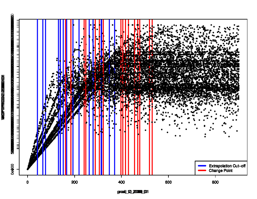
Figure 1: OLYMPUS 25 WOPT output for producer well 2 during the first two years (ending 01/01/2018) versus the corresponding decision input parameter, the target production rate prod_2_2016_01. For small values of prod_2_2016_01 the target is achieved resulting in the perfect linear behaviour up to a change point beyond which the WOPT plateaus as a maximum threshold on the production rate is achieved. The vertical blue and red lines denote the extrapolation cut-off and change point upper bounds respectively.

Throughout this section we focus on emulating outputs for individual ensemble members and thus omit the OLYMPUS model index $j$ for clarity of notation. Let simulator output $f_{i}(\cdot)$ represent an NPV component by well. For the WOPT and WWIT constituents the corresponding decision input parameter which directly affects $f_{i}(\cdot)$ is labelled as $d_{jk,t_{i}}$. In this section the index $i$ is condensed notation for the indices tuple $(jk,t_{i})$, where $j\in\{P,I\}$ refers to the well type ($P$ producer, $I$ injector), $k$ is the well number, and $t_{i}$ is the control interval start date. For each NPV contributor type $l\in\{op,wp,wi\}$, the total over all wells, $Q_{l}(\mathbf{d},t_{i})$ (see Equation 2.3), is obtained via a summation in Equation 4.2, where $N_{l}$ is the number of wells of the relevant type, and $f_{jk,t_{i}}^{l}(\mathbf{d})\equiv f_{i}(\mathbf{d})$ is the quantity for well $k$.

$$Q_{l}(\mathbf{d},t_{i}) {}=\sum_{k=1}^{N_{l}}f_{jk,t_{i}}^{l}(\mathbf{d})$$ (4.2)

4.2.1 Change Points

The target control rate should be adhered to for the duration of the interval. However, this is not always possible due to Bottom Hole Pressure (BHP) constraints suggesting two theoretical distinct modes of behaviour termed the slope and plateau regions. In the slope the target rate is adhered to for the full duration of the control interval, whilst within the plateau region this is not the case. The slope therefore possesses a known gradient which is equal to the length of the control interval, thus $f_{i}(\mathbf{d})=d_{jk,t_{i}}\cdot\Delta t_{i}$. The decision parameter value of transition from slope to plateau is designated the change point and denoted $c_{jk,t_{i}}$. This is unknown, dependent on all other decision parameters, and given only a finite number of simulations is impossible to exactly determine. Consequently, in practical application, there are three distinct regions of behaviour: the slope and plateau separated by an additional uncertain region believed to contain the unknown change point. For a simulator output $f_{i}(\cdot)$ which follows such behaviour the left-hand slope is precisely known up to a tolerance $\delta_{i}\geq 0$; this can be used to estimate the mean change point location given a collection of simulations from design $\mathcal{D}$.

A conservative change point upper bound estimate, $c_{jk,t_{i}}^{u}$, is defined in Equation 4.3, where $f_{i,\mathrm{max}}=\max_{\mathbf{d}\in\mathcal{D}}f_{i}(\mathbf{d})$, and $\delta_{i,u}\geq 0$ is a tolerance included for numerical stability and to ensure that an upper bound is obtained.

$$c_{jk,t_{i}}^{u}=\min_{d_{jk,t_{i}}}\{d_{jk,t_{i}}\mid d_{jk,t_{i}}\cdot\Delta t_{i}\geq f_{i,\mathrm{max}}+\delta_{i,u}\}$$ (4.3)

This is the smallest value of the corresponding decision parameter for which if the target was achieved for the entire control interval, then the simulator output would exceed the largest simulated value (plus a tolerance) over $\mathcal{D}$.

An estimate for the change point lower bound is defined in Section 4.2.1, where $f_{i,\mathrm{diff}}(\mathbf{d})=f_{i,\mathrm{max}}(\mathbf{d})-f_{i}(\mathbf{d})=d_{jk,t_{i}}\cdot\Delta t_{i}-f_{i}(\mathbf{d})$, and $\delta_{i,l}\geq 0$ is another numerical stability tolerance.

$$c_{jk,t}^{l} {}=\dfrac{1}{2}\left(\operatorname*{arg\,min}_{d_{jk,t_{i}}\mid\mathbf{d}\in\mathcal{D}}\{f_{i}(\mathbf{d})<d_{jk,t_{i}}\cdot\Delta t_{i}-\delta_{i,l}\}\right.$$

$${}\phantom{=}\;\left.+\operatorname*{arg\,max}_{d_{jk,t_{i}}\mid\mathbf{d}\in\mathcal{D}}\left\{d_{jk,t_{i}}<\operatorname*{arg\,min}_{d_{jk,t_{i}}\mid\mathbf{d}\in\mathcal{D}}\{f_{i}(\mathbf{d})<d_{jk,t_{i}}\cdot\Delta t_{i}-\delta_{i,l}\}\right\}\right)$$ (4.4)

This is illustrated in Figure 2 for the output WOPTPROD2_20180101 versus the target rate prod_2_2016_01 where the red line represents the slope upper bound if the target is fully adhered to. The vertical blue line denotes $c_{P2,2016}^{l}$ as the midpoint between the first simulation decision parameter setting not on the slope; hence with $f_{i,\mathrm{diff}}(\mathbf{d})>\delta_{i,l}$ (green point; first term in Section 4.2.1), and the decision parameter setting with the largest value of $d_{jk,t_{i}}$ which is less than this first departure point previously obtained (magenta point; second term in Section 4.2.1).

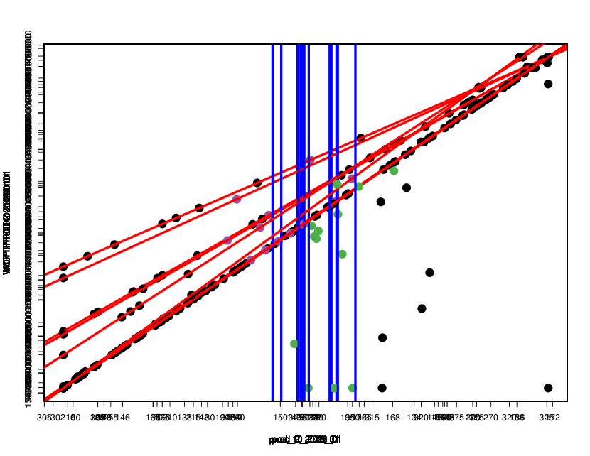
Figure 2: OLYMPUS 25 WOPT for producer well 2 during the first two years (ending 01/01/2018) versus the corresponding target production rate, prod_2_2016_01. The focus on the change point lower bound, $c_{P2,2016}^{l}$, computed using Section 4.2.1, and denoted by the vertical blue line. The red line depicts the slope upper bound attained when the target production rate is adhered to for the full control interval. It is shown that $c_{P2,2016}^{l}$ is the midpoint of the first point not on the slope coloured green, and preceding point which is on the slope coloured magenta.

4.2.2 Extrapolation Cut-Offs

The two distinct modes of behaviour for NPV constituents suggests an emulator be fitted piecewise using a combination of the more accurate knowledge in the slope region, and the less well understood behaviour in the plateau region. Noting the change point location uncertainty, for the plateau region we propose fitting an emulator based only on data which is almost certainly on plateau using the change point upper bound estimate. For $f_{i}(\cdot)$ this is design points with $d_{jk,t_{i}}\geq c_{jk,t_{i}}^{u}$. In order to connect the slope and plateau regions we must extrapolate the plateau emulator. It is necessary to introduce an extrapolation cut-off, denoted $b_{jk,t_{i}}$, beyond which the emulator should not be extrapolated. This is due to limited plateau training data issues. For simulator output $f_{i}(\mathbf{d})$ this is defined with respect to the same decision parameter, $d_{jk,t_{i}}$. The decision space is thus split into three distinct regions:

1. Slope Region: where $d_{jk,t_{i}}<b_{jk,t_{i}}$;

2. Intermediate Region: where $b_{jk,t_{i}}\leq d_{jk,t_{i}}<c_{jk,t_{i}}^{u}$, for which there is uncertainty as to whether simulator output falls on the slope or in the plateau;

3. Plateau Region: where $d_{jk,t_{i}}\geq c_{jk,t_{i}}^{u}$.

There is an estimation trade-off between overly cautious small values which fails to alleviate the above issue, and large values risking points being wrongly classified as on the slope. A suitable and sufficiently conservative approach is to use the change point lower bound, so $b_{jk,t_{i}}=c_{jk,t_{i}}^{l}$ (see Section 4.2.1). The three regions obtained by splitting WOPTPROD2_20180101 versus prod_2_2016_01 at $b_{P2,2016}=c_{P2,2016}^{l}$ and $c_{P2,2016}^{u}$ are illustrated in Figure 1 by the vertical blue and red lines respectively.

4.2.3 Structured Emulation with Upper Truncation

Prior information stipulates that the WOPT and WWIT NPV constituents cannot exceed a maximum (up to a tolerance) determined by the prescribed target rate and control interval length. This upper bound is $d_{jk,t_{i}}\cdot\Delta t_{i}$. Alongside the above parameter space dichotomy, this constraint is imposed through an upper truncation with structured emulators respecting partially known behaviour of these simulator outputs. First a preliminary Bayes linear emulator for $f_{i}(\mathbf{d})$ is fitted using a sub-design, $\mathcal{D}_{i}^{\prime}=\{\mathbf{d}\mid\mathbf{d}\in\mathcal{D},\ d_{jk,t_{i}}>c_{jk,t_{i}}^{u}\}$, with corresponding simulator output $\mathbf{F}_{i}^{\prime}=\{f_{i}(\mathbf{d})\mid\mathbf{d}\in\mathcal{D}_{i}^{\prime}\}$. This represents the behaviour in the plateau region. By construction, all parameter settings in $\mathcal{D}_{i}^{\prime}$ do not adhere to the target rate and hence are in the plateau, thus providing reliable information on which to construct this part of the emulator. This preliminary emulator is only evaluated for $\mathbf{d}$ satisfying $d_{jk,t_{i}}\geq b_{jk,t_{i}}$ and is compared with the upper bound in a classification step determining the structured emulator form:

1. Slope Region: If $d_{jk,t_{i}}<b_{jk,t_{i}}$ or for the preliminary emulator $\operatorname{\mathbb{E}}_{\mathbf{F}_{i}^{\prime}}[f_{i}(\mathbf{d})]-3\sqrt{\operatorname{\mathrm{Var}}_{\mathbf{F}_{i}^{\prime}}[f_{i}(\mathbf{d})]}>d_{jk,t_{i}}\cdot\Delta t_{i}$, then collapse the emulator such that for the structured emulator $\operatorname{\mathbb{E}}_{\mathbf{F}_{i}^{\prime}}[f_{i}(\mathbf{d})]=d_{jk,t_{i}}\cdot\Delta t_{i}$ with fixed maximum absolute errors of size $\delta_{i}$.

2. Intermediate Region: If the preliminary emulator satisfies $\operatorname{\mathbb{E}}_{\mathbf{F}_{i}^{\prime}}[f_{i}(\mathbf{d})]-3\sqrt{\operatorname{\mathrm{Var}}_{\mathbf{F}_{i}^{\prime}}[f_{i}(\mathbf{d})]}\leq d_{jk,t_{i}}\cdot\Delta t_{i}<\operatorname{\mathbb{E}}_{\mathbf{F}_{i}^{\prime}}[f_{i}(\mathbf{d})]+3\sqrt{\operatorname{\mathrm{Var}}_{\mathbf{F}_{i}^{\prime}}[f_{i}(\mathbf{d})]}$, a truncated Gaussian process (truncated GP) emulator is used with mean and variance determined by Equations A.1 and A.2 respectively [24].

3. Plateau Region: In all other cases where $\operatorname{\mathbb{E}}_{\mathbf{F}_{i}^{\prime}}[f_{i}(\mathbf{d})]+3\sqrt{\operatorname{\mathrm{Var}}_{\mathbf{F}_{i}^{\prime}}[f_{i}(\mathbf{d})]}\leq d_{jk,t_{i}}\cdot\Delta t_{i}$, the preliminary emulator output is used.

A structured emulation two-sided truncated variant is also developed and presented in Appendix A, although is unnecessary for the purposes of this application to the TNO OLYMPUS Well Control Optimisation Challenge. Alternative width credible intervals may be used depending on the level of conservativeness desired within an analysis with justification based on the Vysochanskij-Petunin inequality [46].

Compared to using standard Gaussian process or Bayes linear emulators, the above described structured approach yields improved accuracy, along with an increase in speed and efficiency; a consequence of using fewer design points in the fitting. Moreover, both the change point upper bound and extrapolation cut-off estimation processes are computationally very cheap, whilst the use of a truncated GP helps reduce the reliance on accurate estimation of the extrapolation cut-off. The presented methodology is also preferred to alternative partition based emulation approaches for functions with distinct modes of behaviour in different regions of the parameter space such as Treed Gaussian processes [19] because for each NPV constituent the form of the behaviour within the slope region is almost exactly known up to a very small tolerance. This is encapsulated within the developed form of structured emulation. However, treed GPs maintain a much larger uncertainty over this region than necessary, whilst struggling when the number of design points within each region is relatively limited impacting further on the treed GP accuracy. This consideration has implications during subsequent (decision) analyses.

Each NPV constituent is emulated separately by well before combining in a “divide and conquer approach” to obtain an overall emulator of improved accuracy. The emulator adjusted expectation and variance for $Q_{j,op}(\mathbf{d},t_{i})$, $Q_{j,wp}(\mathbf{d},t_{i})$, and $Q_{j,wi}(\mathbf{d},t_{i})$ in Equation 2.3 are shown in Equations 4.5 and 4.6 respectively, where $\mathbf{F}_{j}$ represents all data used to fit the NPV constituents emulators for OLYMPUS model $j$.

$$\operatorname{\mathbb{E}}_{\mathbf{F}}\left[Q_{l}(\mathbf{d},t_{i})\right] {}=\sum_{k=1}^{N_{l}}\operatorname{\mathbb{E}}_{\mathbf{F}}\left[f_{jk,t_{i}}^{l}(\mathbf{d})\right]$$ (4.5)

$$\operatorname{\mathrm{Var}}_{\mathbf{F}}\left[Q_{l}(\mathbf{d},t_{i})\right] {}=\sum_{k=1}^{N_{l}}\operatorname{\mathrm{Var}}_{\mathbf{F}}\left[f_{jk,t_{i}}^{l}(\mathbf{d})\right]$$ (4.6)

4.3 Emulation of the Approximate NPV

An intuitive means of combining emulators for the NPV constituents is via the NPV formula in Equations 2.1 and 2.3. However, control intervals are often formed by amalgamating multiple consecutive discounting intervals, hence the constituent emulators do not correspond exactly to the terms in the NPV formula, labelled as the exact NPV, and denoted by $\mathrm{NPV}_{j}(\mathbf{d})$ for the $j$^th model. A formula for an approximate NPV, denoted $\widetilde{\mathrm{NPV}}_{j}(\mathbf{d})$, is presented in Equation 4.7, where $\lambda_{i}$ is a weighted average discounting factor for the $i$^th interval defined in Equation 4.8 for which $k$ indexes the discounting intervals contained within the longer control interval, $N_{t_{i}}$ is the total number of such discounting intervals, and $t_{i,0}=t_{i-1}$.

$$\widetilde{\mathrm{NPV}}_{j}(\mathbf{d}) {}=\sum_{i=1}^{N_{t}}\lambda_{i}\left[Q_{j,op}(\mathbf{d},t_{i})\cdot r_{op}-Q_{j,wp}(\mathbf{d},t_{i})\cdot r_{wp}-Q_{j,wi}(\mathbf{d},t_{i})\cdot r_{wi}\right]$$ (4.7)

$$\lambda_{i} {}=\dfrac{1}{t_{i}-t_{i-1}}\sum_{k=1}^{N_{t_{i}}}\dfrac{t_{i,k}-t_{i,k-1}}{(1+d)^{\frac{t_{i,k}}{\tau}}}$$ (4.8)

Note that using an averaged discount factor yields a more accurate approximation compared with applying the discounting at the end of the control intervals only.

An emulator for $\mathrm{NPV}_{j}(\mathbf{d})$ is obtained by substituting the simulator for emulators of $Q_{j,op}(\mathbf{d},t_{i})$, $Q_{j,wp}(\mathbf{d},t_{i})$ and $Q_{j,wi}(\mathbf{d},t_{i})$ using Equations 4.5 and 4.6. Assuming uncorrelated NPV constituents, and using a collection of univariate emulators, Equations 4.9 and 4.10 are the adjusted expectation and variance formulae respectively. As above, $\mathbf{F}_{j}$ represents all data used to fit the NPV constituents emulators for the $j$^th ensemble member.

$$\operatorname{\mathbb{E}}_{\mathbf{F}_{j}}\left[\widetilde{\mathrm{NPV}}_{j}(\mathbf{d})\right] {}=\sum_{i=1}^{N_{t}}\lambda_{i}\left\{r_{op}\operatorname{\mathbb{E}}_{\mathbf{F}_{j}}[Q_{j,op}(\mathbf{d},t_{i})]\right.$$

$${}\phantom{=}\;\phantom{\sum_{i=1}^{N_{t}}\lambda_{i}\left\{\right.}\left.-r_{wp}\operatorname{\mathbb{E}}_{\mathbf{F}_{j}}[Q_{j,wp}(\mathbf{d},t_{i})]-r_{wi}\operatorname{\mathbb{E}}_{\mathbf{F}_{j}}[Q_{j,wi}(\mathbf{d},t_{i})]\right\}$$ (4.9)

$$\operatorname{\mathrm{Var}}_{\mathbf{F}_{j}}\left[\widetilde{\mathrm{NPV}}_{j}(\mathbf{d})\right] {}=\sum_{i=1}^{N_{t}}\lambda_{i}^{2}\left\{r_{op}^{2}\operatorname{\mathrm{Var}}_{\mathbf{F}_{j}}[Q_{j,op}(\mathbf{d},t_{i})]\right.$$

$${}\phantom{=}\;\phantom{\sum_{i=1}^{N_{t}}\lambda_{i}^{2}\left\{\right.}\left.+r_{wp}^{2}\operatorname{\mathrm{Var}}_{\mathbf{F}_{j}}[Q_{j,wp}(\mathbf{d},t_{i})]+r_{wi}^{2}\operatorname{\mathrm{Var}}_{\mathbf{F}_{j}}[Q_{j,wi}(\mathbf{d},t_{i})]\right\}$$ (4.10)

For each WOPT and WWIT contributor where structured emulation is applied, for new $\mathbf{d}$ identified as either in the plateau region or the uncertain region around the change point, the adjusted expectation and variance are obtained from the preliminary Bayes linear or truncated GP emulator respectively. In the slope region where the emulator is collapsed onto the slope, the expectation is known whilst the adjusted variance is approximated by treating $\delta_{i}$ as equal to 3 standard deviations. Since the WWPT constituents do not adhere to the structured mode of behaviour, these are emulated using a Bayes linear emulator.

4.4 Linking the Exact and Approximate NPV

There exists a very strong linear relationship between the approximate and exact NPV for which a simple linear regression in Equation 4.11 provides a meaningful statistical link whilst capturing the additional induced uncertainties.

$$\mathrm{NPV}_{j}(\mathbf{d})=\beta_{0,\widetilde{\mathrm{NPV}}_{j}}+\beta_{1,\widetilde{\mathrm{NPV}}_{j}}\widetilde{\mathrm{NPV}}_{j}(\mathbf{d})+\varepsilon_{\widetilde{\mathrm{NPV}}_{j}}$$ (4.11)

The adjusted expectation and variance are then computed using Equations 4.12 and 4.13 respectively. Estimates of the regression coefficients, $\hat{\beta}_{0,\widetilde{\mathrm{NPV}}_{j}}$ and $\hat{\beta}_{1,\widetilde{\mathrm{NPV}}_{j}}$, along with their variances and covariance, are obtained using the wave 0 simulation data, whilst $\varepsilon_{\widetilde{\mathrm{NPV}}_{j}}$ is treated as independent with residual standard error $\sigma_{\widetilde{\mathrm{NPV}}_{j}}$.

$$\operatorname{\mathbb{E}}_{\mathbf{F}_{j}}[\mathrm{NPV}_{j}(\mathbf{d})] {}=\hat{\beta}_{0,\widetilde{\mathrm{NPV}}_{j}}+\hat{\beta}_{1,\widetilde{\mathrm{NPV}}_{j}}\operatorname{\mathbb{E}}_{\mathbf{F}_{j}}\left[\widetilde{\mathrm{NPV}}_{j}(\mathbf{d})\right]$$ (4.12)

$$\operatorname{\mathrm{Var}}_{\mathbf{F}_{j}}[\mathrm{NPV}_{j}(\mathbf{d})] {}=\operatorname{\mathrm{Var}}\left[\hat{\beta}_{0,\widetilde{\mathrm{NPV}}_{j}}\right]+2\operatorname{\mathrm{Cov}}\left[\hat{\beta}_{0,\widetilde{\mathrm{NPV}}_{j}},\hat{\beta}_{1,\widetilde{\mathrm{NPV}}_{j}}\right]\operatorname{\mathbb{E}}_{\mathbf{F}_{j}}\left[\widetilde{\mathrm{NPV}}_{j}(\mathbf{d})\right]$$

$${}\phantom{=}\;+\left\{\hat{\beta}_{1,\widetilde{\mathrm{NPV}}_{j}}^{2}+\operatorname{\mathrm{Var}}\left[\hat{\beta}_{1,\widetilde{\mathrm{NPV}}_{j}}\right]\right\}\operatorname{\mathrm{Var}}_{\mathbf{F}_{j}}\left[\widetilde{\mathrm{NPV}}_{j}(\mathbf{d})\right]$$

$${}\phantom{=}\;+\operatorname{\mathrm{Var}}\left[\hat{\beta}_{1,\widetilde{\mathrm{NPV}}_{j}}\right]\left(\operatorname{\mathbb{E}}_{\mathbf{F}_{j}}\left[\widetilde{\mathrm{NPV}}_{j}(\mathbf{d})\right]\right)^{2}+\sigma_{\widetilde{\mathrm{NPV}}_{j}}^{2}$$ (4.13)

4.5 Emulation of the Ensemble Mean NPV

The objective is to emulate the ensemble mean NPV by combining emulators for individual models. A reasonable assumption is that the ensemble members are independent given the complexity of their different underlying geologies.

4.5.1 When Simulations are Available for all Ensemble Members

When simulations are relatively quick to evaluate; large amounts of computing resources are available; or there is a desire to minimise the uncertainty (here due to the underlying geology, which is particularly relevant when the ensemble mean NPV is assumed equal to the expected NPV), it may be possible to simulate from the entire ensemble. The ensemble mean NPV is computed as either the arithmetic or a weighted mean (with weights obtained from a prior probability model over the geologies) of the individual model NPVs. This presents a natural method to emulate $\overline{\mathrm{NPV}}$ with the adjusted expectation and variance defined in Equations 4.14 and 4.15, where $\mathbf{F}$ denotes all necessary simulation data, and weights $\omega_{j}$, with $\omega_{j}=\frac{1}{N}$ for the arithmetic mean.

$$\operatorname{\mathbb{E}}_{\mathbf{F}}\left[\overline{\mathrm{NPV}}(\mathbf{d})\right] {}=\sum_{j=1}^{N}\omega_{j}\operatorname{\mathbb{E}}_{\mathbf{F}_{j}}[\mathrm{NPV}_{j}(\mathbf{d})]$$ (4.14)

$$\operatorname{\mathrm{Var}}_{\mathbf{F}}\left[\overline{\mathrm{NPV}}(\mathbf{d})\right] {}=\sum_{j=1}^{N}\omega_{j}^{2}\operatorname{\mathrm{Var}}_{\mathbf{F}_{j}}[\mathrm{NPV}_{j}(\mathbf{d})]$$ (4.15)

The variance formula may be adapted when different model NPVs are believed to be correlated by introducing the relevant covariance terms in Equation 4.15.

4.5.2 Using the Ensemble Subsampling Linear Model

A more realistic and practical scenario is that simulations are only performed for a subset of the ensemble, such as selected using the techniques described in Section 4.1. The linear model in Equation 4.1 is used to emulate $\overline{\mathrm{NPV}}$ with the emulated NPV for each of the sub-selected models as inputs. The estimated coefficients are denoted by $\hat{\alpha}_{\mathrm{ES}}$ and $\hat{\beta}_{k,\mathrm{ES}}$. It is assumed that the individual emulator outputs and the regression coefficients are uncorrelated, which is justifiable if two distinct simulation data sets are used to construct the linear model and fit the emulators. Under this formulation the adjusted expectation is shown in Equation 4.16.

$$\operatorname{\mathbb{E}}_{\mathbf{F}}\left[\overline{\mathrm{NPV}}(\mathbf{d})\right] {}=\operatorname{\mathbb{E}}_{\mathbf{F}}\left[\hat{\alpha}_{\mathrm{ES}}+\sum_{k=1}^{\tilde{N}}\hat{\beta}_{k,\mathrm{ES}}\mathrm{NPV}_{j_{k}}(\mathbf{d})+\varepsilon_{\mathrm{ES}}(\mathbf{d})\right]$$

$${}=\hat{\alpha}_{\mathrm{ES}}+\sum_{k=1}^{\tilde{N}}\hat{\beta}_{k,\mathrm{ES}}\operatorname{\mathbb{E}}_{\mathbf{F}_{j_{k}}}[\mathrm{NPV}_{j_{k}}(\mathbf{d})]$$ (4.16)

Define $\hat{\boldsymbol{\beta}}_{\mathrm{ES}}=(\hat{\alpha}_{\mathrm{ES}},\hat{\beta}_{1,\mathrm{ES}},\ldots,\hat{\beta}_{\tilde{N},\mathrm{ES}})^{\mathrm{T}}\in\mathbb{R}^{\tilde{N}+1}$ with $\Sigma_{\beta,\mathrm{ES}}=\operatorname{\mathrm{Var}}\left[\hat{\boldsymbol{\beta}}_{\mathrm{ES}}\right]$, and $X_{\mathrm{ES}}(\mathbf{d})=(1,\mathrm{NPV}_{j_{1}}(\mathbf{d}),\ldots,\mathrm{NPV}_{j_{\tilde{N}}}(\mathbf{d}))^{\mathrm{T}}\in\mathbb{R}^{\tilde{N}+1}$ with uncorrelated components, so $\operatorname{\mathrm{Var}}_{\mathbf{F}}\left[X_{\mathrm{ES}}(\mathbf{d})\right]$ is diagonal. The adjusted variance is presented in Equation 4.17, where $\hat{\sigma}_{\mathrm{ES}}$ is the estimated residual standard error for $\varepsilon_{\mathrm{ES}}(\mathbf{d})$.

$$\operatorname{\mathrm{Var}}_{\mathbf{F}}\left[\overline{\mathrm{NPV}}(\mathbf{d})\right] {}=\operatorname{\mathrm{Var}}\left[\hat{\alpha}_{\mathrm{ES}}\right]$$

$${}\phantom{=}\;+\sum_{k=1}^{\tilde{N}}\operatorname{\mathrm{Var}}\left[\hat{\beta}_{k,\mathrm{ES}}\right]\left(\operatorname{\mathrm{Var}}_{\mathbf{F}_{j_{k}}}\left[\mathrm{NPV}_{j_{k}}(\mathbf{d})\right]+\operatorname{\mathbb{E}}_{\mathbf{F}_{j_{k}}}\left[\mathrm{NPV}_{j_{k}}(\mathbf{d})\right]^{2}\right)$$

$${}\phantom{=}\;+2\sum_{k=1}^{\tilde{N}}\operatorname{\mathrm{Cov}}\left[\hat{\alpha}_{\mathrm{ES}},\hat{\beta}_{k,\mathrm{ES}}\right]\operatorname{\mathbb{E}}_{\mathbf{F}_{j_{k}}}\left[\mathrm{NPV}_{j_{k}}(\mathbf{d})\right]$$

$${}\phantom{=}\;+\sum_{\begin{subarray}{c}k\neq l\\ k,l=1,\ldots,\tilde{N}\end{subarray}}\left(\operatorname{\mathrm{Cov}}\left[\hat{\beta}_{k,\mathrm{ES}},\hat{\beta}_{l,\mathrm{ES}}\right]\right.$$

$${}\phantom{=}\;\phantom{+\sum_{\begin{subarray}{c}k\neq l\\ k,l=1,\ldots\tilde{N}\end{subarray}}\left(\right.}\left.\cdot\operatorname{\mathbb{E}}_{\mathbf{F}_{j_{k}}}\left[\mathrm{NPV}_{j_{k}}(\mathbf{d})\right]\operatorname{\mathbb{E}}_{\mathbf{F}_{j_{l}}}[\mathrm{NPV}_{j_{l}}(\mathbf{d})]\right)$$

$${}\phantom{=}\;+\sum_{k=1}^{\tilde{N}}\hat{\beta}_{k}^{2}\operatorname{\mathrm{Var}}_{\mathbf{F}_{j_{k}}}[\mathrm{NPV}_{j_{k}}(\mathbf{d})]+\hat{\sigma}_{\mathrm{ES}}^{2}$$ (4.17)

5 Results

The statistical methodology presented in Section 4 is demonstrated for the motivating TNO OLYMPUS Well Control Optimisation Challenge introduced in Section 2, which is reformulated as a decision support problem with a focus on the ensemble mean NPV, $\overline{\mathrm{NPV}}(\mathbf{d})\approx\operatorname{\mathbb{E}}[\mathrm{NPV}](\mathbf{d})$. This builds on the work published in [32]. This includes: an exploratory design of simulations and analysis in Section 5.1; subsampling from the OLYMPUS ensemble in Section 5.2; an efficient method for constructing a targeted Bayesian design in Section 5.3; application of Bayes linear and the proposed hierarchical emulator to the ensemble mean NPV in Sections 5.4 and 5.5; with a comparison performed in Section 5.6.

5.1 OLYMPUS Exploratory Analysis

We first construct a maximum Latin hypercube design and run a wave 0 of $n=20$ exploratory simulations using all $N=50$ OLYMPUS models. An important feature is the adherence of OLYMPUS simulations to target production and injection rate decision parameters. For one vector of decision parameter settings Figure 3 compares the input target control rates (black dashed lines) with the corresponding outputted achieved rates over the 50 ensemble members (coloured traces). It is immediately evident in all plots that the input targets are not strictly adhered to for the full duration of the control intervals; a consequence of the underlying physics programmed into the OLYMPUS model, including constraints on BHP, resulting in such deviations between the actual and targetted control values. It is this behaviour which motivates our structured emulation approach in Section 4.2 which is demonstrated in Section 5.5.1. Another interesting facet with potential ramifications for emulation and decision support is the vastly different relative absolute contributions of oil and water to the NPV objective function. An assessment is shown in Figure 11, along with further discussion in Section B.1.

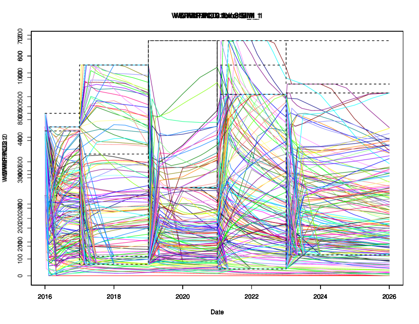
(a) WOPR.PROD.2.

(b) WOPR.PROD.10.

(c) WWIR.INJ.2.

(d) WWIR.INJ.3.

Figure 3: Comparison of the target and achieved control rate decision parameters for an OLYMPUS wave 0 exploratory simulation over the full multi-model ensemble. Plots show the OLYMPUS output actual control rates time series as coloured lines for each ensemble member for the Well Oil Production Rates (WOPR, top) or Well Water Injection Rates (WWIR, bottom) for the four wells within the CWG. The black dashed lines that show the corresponding decision parameters of target production or injection rates respectively. The differences between the output traces and the inputs highlights the deviations between the target control and what is achieved due to physical constraints applied in the model.

5.2 Subsampling from Geological Multi-Model Ensemble

A preliminary graphical investigation is performed using plots of the ensemble mean versus individual model for a range of outputs of interest for the exploratory simulations. Examples are provided in Figure 12 (see Section B.2). It is unnecessary to sub-select models exhibiting close individual model output relations with the ensemble mean. Instead we screen for cases where the relationship is easy to model, for example, with a preference for linear associations with small output variation, identifying an initial set of 9 OLYMPUS models for further exploration via linear modelling. Further discussion is found in Section B.2, and in [31, Sec. 4.2].

In order to capture the interacting effects of the different OLYMPUS models, the subsampling technique utilising the linear model in Equation 4.1 is implemented. First it is applied to the proposed OLYMPUS subset before extending to all models via both directions stepwise selection starting from the full model and using AIC as the model selection criterion. It is established that a subset of only $\tilde{N}=3$ models is sufficient for a large number of the investigated outputs, yielding high Adjusted $R^{2}$ values shown in Figure 13 in Section B.2. The optimal collection for the ensemble mean NPV is OLYMPUS 25, 33, & 45. The fitted linear model provides an efficient means of prediction and uncertainty quantification by using only 3 ensemble members yielding substantial computational savings. This is a novel application of such multi-model ensemble subsampling techniques in petroleum reservoir engineering.

5.3 Targeted Bayesian Design of Simulations

We employ a novel targeted Bayesian design method, based on that presented in [32] and [31, Sec. 4.3], which is tailored to performing decision support through targeted sampling based on prior beliefs of experienced petroleum reservoir engineers regarding the location of optimal decision parameter settings, as well as imposing practical and physical constraints. Firstly, TNO stipulate operational range constraints to be $[0,900]$m³/day and $[0,1600]$m³/day for production and injection rates respectively; leading to a 32-dimensional hypercube parameter space. Oil reservoir engineers deem large temporal variation in controls to be unphysical and poor practice, thus suggesting a difference constraint between time consecutive controls. The 32 decision inputs are therefore split into four independent subgroups by well with difference constraint $\lvert d_{jk,t_{i}}-d_{jk,t_{i}-1}\rvert\leq\Delta_{i},\ i=2,\ldots,D^{(jk)}$, where $D^{(jk)}=8$ is the number of control intervals for well $jk$. A conservative choice is that the maximum permitted change over a two year time interval is $\Delta_{i}=\frac{1}{3}$ of the operational range for the well type. Consequently the decision parameter space is no longer a hypercube with a volume of 3.45% of the initial hypercube due to the range constraints only.

The targeted Bayesian design algorithm is implemented to generate a $n=700$ point design. First, for each of the above four subgroups of eight decision parameters the normalised parameter sums are sampled from a truncated normal distribution in order to facilitate the exploration of more extreme values of the total sums of the eight normalised parameters than would be the case using a standard uniform or Latin hypercube design. This is perceived to be important based on reservoir engineering insight. Next, the differences are sampled according to the specified value of $\Delta_{i}$ before imposing the operational range constraints (after transforming the normalised parameters to their physical values). Each parameter subgroup and the overall design are approximately optimised with respect to the minimax design selection criterion by comparing candidate designs to a large $20,000$ point uniform random sample (over the constrained parameter space) [38]. Moreover, the optimised design is augmented to include two further decision parameter vectors with all parameters set to either their minimum or maximum values since it is of interest to observe the model behaviour at these extremes. Full details of the targeted Bayesian design algorithm are presented in Section B.3.

The final wave 1 design for eight producer well 2 parameters is illustrated in Figure 4. The plots next to the diagonal highlights the difference constraints as points are clustered between two clearly defined diagonal parallel bounds. Since the final two control intervals are of length 4 years a greater change of up to $\frac{2}{3}$ of the parameter operational range is permitted, hence the wider bands. In addition, the difference constraints affect decision parameters at larger time separations where there are fewer points away from the diagonal, although is less pronounced for greater time gaps. This design is evaluated for the identified subset of 3 OLYMPUS models with the linear model used to predict the ensemble mean NPV for which points are coloured green, yellow and red for high, moderate and low NPVs respectively in Figure 4.

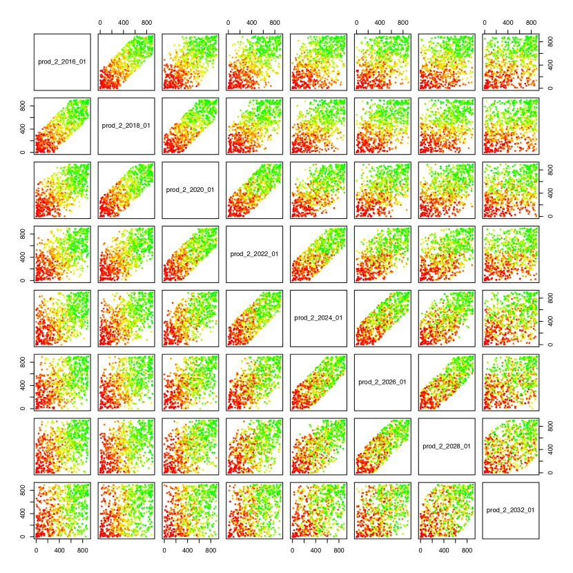
Figure 4: Wave 1 702 point design OLYMPUS producer well 2 decision parameters pairs plots. Points are coloured by the multi-model ensemble subsampling linear model predicted NPV where green, yellow and red correspond to high, moderate and low NPVs respectively.

Note that the presented emulation methodology also works with more traditional space filling designs. Employment of a targeted Bayesian design is to enhance the overall decision support aim, and to incorporate expert knowledge regarding the reservoir behaviour and practical decision implementation.

5.4 Bayes Linear Emulation of the Expected NPV

Bayes linear emulation is directly applied to the expected NPV to explore the 32-dimensional wave 1 decision parameter space utilising the above design and linear model predictions for the ensemble mean NPV for training and validation. This serves as a comparison with our proposed hierarchical emulation approach in Section 5.6. Following the methodology summarised in Section 3, an emulator with a nugget term (see Section 3) is employed with $f(\mathbf{d})=U(\mathbf{d})=\operatorname{\mathbb{E}}[\mathrm{NPV}](\mathbf{d})$. Investigations using linear modelling, stepwise selection with the AIC criterion, and with all parameters transformed onto $[-1,1]$, as in [41], yields a subset of 12 active decision parameters and a suggested second-order polynomial mean function form:

$$\operatorname{\mathbb{E}}[\mathrm{NPV}](\mathbf{d}_{A_{\mathrm{BL}}})=\beta_{0}+\sum_{d_{i}\in A_{\mathrm{BL}}}\{\beta_{i,1}d_{i}+\beta_{i,2}d_{i}^{2}\}+\varepsilon$$ (5.1)

The residual uncertainty is captured through $\varepsilon$ which possesses an estimate residual standard error $\sigma_{lm}$. The unknown regression coefficients are assumed to have prior expectation $\boldsymbol{\mu}_{\beta}=\mathbf{0}$ and an infinite prior uncertainty, with emulator updates exploiting limiting results as $\operatorname{\mathrm{Var}}[\boldsymbol{\beta}]\rightarrow\infty$ for which formulae are presented in [32, Sec. 2.4.5].

For the residual process it is assumed that $\operatorname{\mathbb{E}}[u(\mathbf{d}_{A_{\mathrm{BL}}})]=0$ and $\operatorname{\mathbb{E}}[w(\mathbf{d})]=0$ with a squared exponential covariance structure (Equation 3.2) using a single common correlation length hyperparameter. Following the substitution approach for the hyperparameters: $\sigma_{u}^{2}=(1-\rho)\sigma_{lm}^{2}$ and $\sigma_{w}^{2}=\rho\sigma_{lm}^{2}$ where $\rho=0.05$; whilst the correlation length parameter is set to half of the parameter range, hence $\theta=1$. These choices are validated via emulator diagnostics discussed below. Bayes linear emulator adjustment is performed using Equations 3.4, 3.5 and 3.6.

Leave-one-out diagnostics suggest that the emulator fits well across the decision space, as shown in Figure 5 of the adjusted expectation with an approximate 95% credible interval of width 3 adjusted standard deviations (following Pukelsheim’s 3-sigma rule [33]) versus the expected NPV. 691 of the 702 (98.4%) credible intervals contain the simulated expected NPV, as highlighted by the red dashed line representing equality. Moreover, if we instead employed a Gaussian process emulator, then the 95% credible intervals contain 679 of the simulated expected NPVs; a 96.7% coverage. It is noted that the few cases where these diagnostics are not satisfied tend to yield over-prediction. With a view to decision support this is less of a concern as these regions will not be incorrectly ruled out due to low expected NPVs, while iterative refinement enables more accurate emulation at later waves.

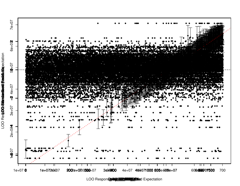
Figure 5: Bayes linear emulator for the expected NPV leave-one-out diagnostics plot showing the emulator adjusted expectations with 95% 3 adjusted standard deviation credible interval error bars versus the simulated expected NPV. The red dashed line denotes equality of the emulator prediction and the simulator output.

5.5 Hierarchical Emulation of the Expected NPV

We present an application of our hierarchical emulation framework to the TNO OLYMPUS Well Control Optimisation Challenge for the decision support setup outlined in Section 2. As for Bayes linear emulation, this analysis utilises the ensemble subsampling linear model to predict the expected NPV using only 3 geological realisations, as described in Section 5.2, along with the design constructed in Section 5.3.

5.5.1 Structured Emulation of the NPV Constituents

For each OLYMPUS model the NPV is determined by the oil production, water injection and production. We therefore decompose the NPV calculation into WOPT, WWIT, and WWPT, by both model and control interval. As discussed, the WOPT and WWIT within a control interval are observed to follow structured behaviour where the quantity is equal to the corresponding target rate decision parameter multiplied by the length of the time interval up to an unknown change point beyond which there is a plateau in the behaviour due to the BHP constraint. This is illustrated for the OLYMPUS 25 WOPT for producer well 2 over the first two year control interval (01/01/2016 to 01/01/2018) in Figure 1 which we use as a running example. We therefore employ the structured emulation technique of Section 4.2 separately for each of the WOPT and WWIT within control interval constituents for wells in the CWG. Conservative change points upper bounds and extrapolation cut-offs are estimated using Equations 4.3 and 4.2.1 respectively over the wave 1 simulations, with tolerances $\delta_{i,u}=\delta_{i,l}=10$ chosen to ensure numerical stability. Figure 14 (in Section B.4) depicts the regions in which the “true” change points are believed to be situated for all WOPT and WWIT for each of the three wave 1 OLYMPUS models.

For each NPV constituent the next stage is to fit a preliminary Bayes linear emulator where the deterministic functions of the active decision parameters are:

$$m_{i}(\mathbf{d}_{A_{i}})=\mathbf{g}_{i}(\mathbf{d}_{A_{i}})^{\mathrm{T}}\boldsymbol{\beta}_{i}=\beta_{i,0}+\sum_{d_{j}\in A_{i}}\{\beta_{i,j,1}d_{j}+\beta_{i,j,2}d_{j}^{2}\}$$ (5.2)

It is assumed that the active decision parameters comprise all decisions which take place in the past of the output. For our running example this is $A_{i}=\{$prod_2_2016_01, prod_10_2016_01, inj_2_2016_01, inj_3_2016_01$\}$. This is a logical choice since future decisions are physically unable to impact on an output up to the current time, however any past decisions may potentially have an effect. The remainder of each emulator’s prior specification is analogous to in Section 5.4, but with the distinction that only those simulation points in $\mathcal{D}_{i}^{\prime}=\{\mathbf{d}\mid\mathbf{d}\in\mathcal{D},\ d_{jk,t_{i}}>c_{jk,t_{i}}^{u}\}$ with output $\mathbf{F}_{i}^{\prime}=\{f_{i}(\mathbf{d})\mid\mathbf{d}\in\mathcal{D}_{i}^{\prime}\}$ are used in the fitting.

For our example of the OLYMPUS 25 WOPT for producer well 2 in the first control interval (ending 01/01/2018) the preliminary emulator predictive 3-sigma credible intervals are illustrated in Figure 6(a) versus the corresponding decision parameter, prod_2_2016_01. This is compared to the theoretical maximum output depicted by the black dotted line determined by the effective target rate for the control interval. The vertical blue and red lines are situated at $b_{P2,2016}$ and $c_{P2,2016}^{u}$ respectively. The structured emulation methodology using an upper truncation yields the results shown in Figure 6(b). Within the slope region, shown in purple, the preliminary emulator credible intervals exceed the constraint and are thus collapsed onto the slope yielding very narrow intervals representing strong beliefs that these decisions will be adhered to for the full control interval. Included are all decision parameter vectors with $d_{P2,2016}<b_{P2,2016}$, as well as cases where $d_{P2,2016}\geq b_{P2,2016}$ in which the preliminary emulator credible interval lower bound exceeds the slope. The uncertain intermediate region, shown in orange, is handled by a truncated GP reflecting the uncertainty in whether the model output is on the slope or relatively close when a target rate is achieved for the majority of a control interval. All of these points lie close to the black dotted slope line with much narrower credible intervals than the preliminary Bayes linear emulator. For the plateau region, shown in green, the preliminary emulator credible interval is well below this slope. It is therefore unnecessary to impose a truncation due to the very small probability that an emulator realisation actually exceeds this physical constraint, hence these intervals are unchanged between the two plots.

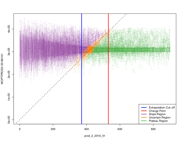
(a) Preliminary Bayes linear emulator predictive CI versus prod_2_2016_01.

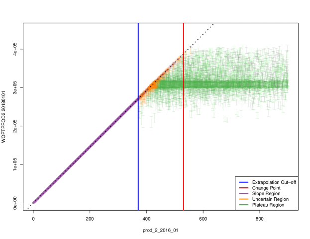
(b) Structured emulator with upper truncation predictive CI versus prod_2_2016_01.

Figure 6: OLYMPUS 25 wave 1 WOPT for producer well 2 during the first two years (ending 01/01/2018) versus the corresponding target production rate, prod_2_2016_01. The top plot shows the wave 1 preliminary Bayes linear emulator predictive 3-sigma credible interval (CI) fitted using only the simulations with $d_{P2,2016}\geq c_{P2,2016}^{u}$. This is used within the structured emulation algorithm imposing the upper truncation due to the slope (black dotted line) with the CI shown in the bottom plot. The vertical blue and red lines are situated at $b_{P2,2016}$ and $c_{P2,2016}^{u}$ respectively. The purple, orange and green CI correspond to points in the slope, uncertain, and plateau regions respectively.

Leave-one-out structured emulator diagnostics demonstrate satisfactory results with examples shown in Figure 7 for OLYMPUS 25 NPV constituents WOPT and WWIT in the control intervals ending 01/01/2018 and 01/01/2022 respectively. The first is our running example.

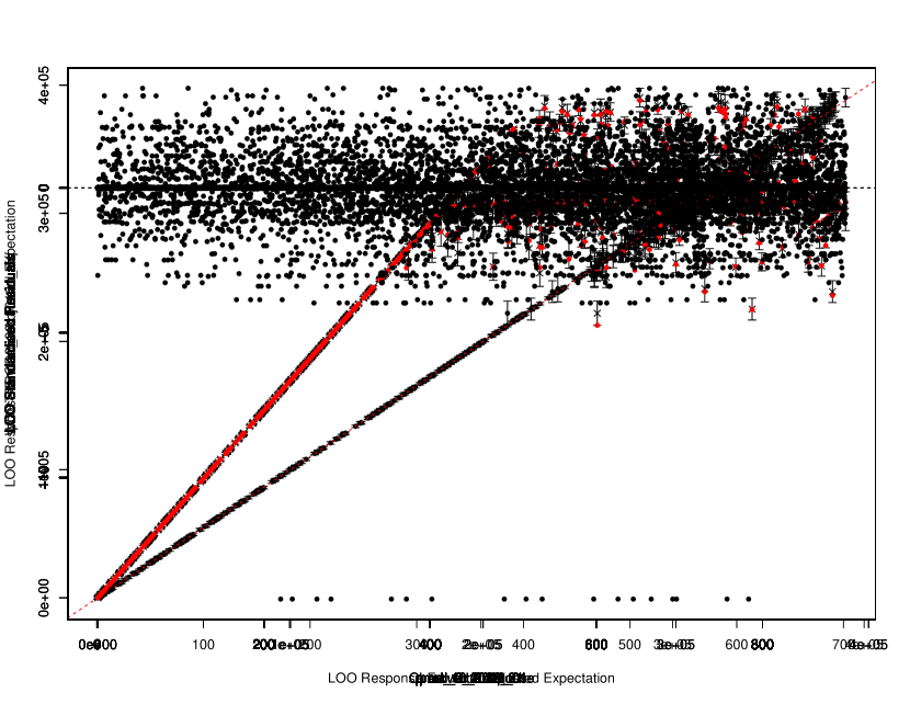
(a) WOPTPROD2_2018_01 emulator CI versus simulated output.

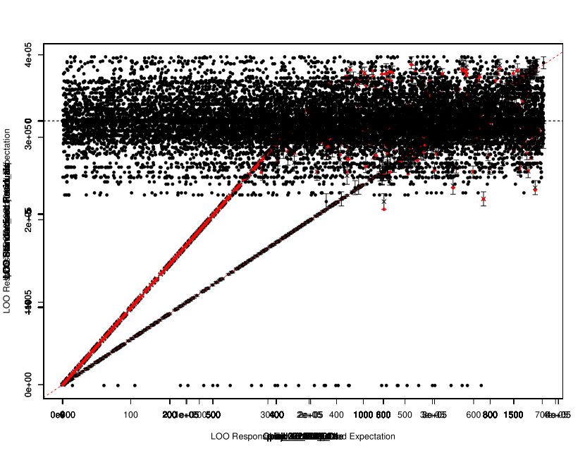
(b) WOPTPROD2_2018_01 emulator CI versus prod_2_2016_01.

(c) WWITINJ2_2022_01 emulator CI versus simulated output.

(d) WWITINJ2_2022_01 emulator CI versus inj_2_2020_01.

Figure 7: Structured emulation leave-one-out diagnostic plots for OLYMPUS 25 WOPTPROD2_2018_01 (top) and WWITINJ2_2022_01 (bottom). Left: Adjusted expectation with 95% credible intervals (CI) of width 3 adjusted standard deviations versus the simulated value. The red dashed line denotes equality of the emulator and simulator. Right: Credible interval versus the output’s corresponding target production and injection rate respectively. Red points denote the simulated output.

Figures 7(a) and 7(c) show the emulator adjusted expectation with 95% (3 adjusted standard deviations) credible intervals versus the simulated output. In each case the emulator is exceptionally accurate for smaller NPV constituent values corresponding to where the target rate is adhered to for the entire control interval. For larger simulated outputs believed to be on plateau, the credible interval is wider, whilst the use of a truncated GP emulator for intermediate values demonstrates a reduction in the uncertainty in these locations. The classification step emulator type is best observed in Figures 7(b) and 7(d) of the credible intervals versus each NPV constituents’ corresponding decision parameter. For all NPV constituents the majority of the credible intervals contain the simulated value and no issues are detected in other leave-one-out diagnostic analyses. This demonstrates how incorporating known structures within the emulator enables very accurate emulators for the WOPT and WWIT NPV constituents based on a relatively small number of simulations whilst also capturing the change in behaviour.

Structured behaviour is not observed for WWPT within a control interval since there is no corresponding target rate; its behaviour is a consequence of attempting to achieve a given target production rate subject to BHP constraints with water present within the oil field. We separately employ Bayes linear emulators for the WWIT following the same approach as above, but fitted using all simulations in $\mathcal{D}$.

5.5.2 Emulation of the OLYMPUS Approximate NPV

In this application the 8 decisions for each well are enacted over periods constructed by amalgamating consecutive 3-month discounting intervals. Emulation of the average discounting approximate NPV (Equation 4.7) for each OLYMPUS model is performed as described in Section 4.3 with leave-one-out diagnostics plots for the OLYMPUS 25 approximate NPV shown in Figure 8(a). There exists a strong linear relation between the emulator adjusted expectation and the simulated approximate NPV with the majority of points situated close to the red dashed equality line. It is observed that the uncertainty generally increases with the value of the approximate NPV. Petroleum reservoir engineering provides insight: higher target production and injection rates are generally necessary to achieve the largest NPVs. For the WOPT and WWIT structured emulators this occurs above the extrapolation cut-off and thus each constituent emulator exhibits a larger uncertainty. Furthermore, when many of the NPV constituents fall in their slope regions the structured emulator returns a small uncertainty determined by the tolerance. These linearly combine to produce a small uncertainty for the approximate NPV.

(a) Approx NPV CI versus simulated values.

(b) Exact NPV CI versus simulated values.

Figure 8: Emulator leave-one-out diagnostic plots for OLYMPUS 25 average discounting approximate NPV (left) and exact NPV (right, obtained via the linear model in Equation 4.11 on the emulated approximate NPV) showing the adjusted expectation with 3 adjusted standard deviation Credible Intervals (CI) versus simulated values. The red dashed line denotes when the emulator and simulator coincide.

5.5.3 Linking the OLYMPUS Exact and Approximate NPV

The next step within the hierarchical emulator construction is to link the exact and approximate NPV for each OLYMPUS model. This accounts for the discrepancy induced by coalescing the discounting intervals. This follows the simple linear regression framework in Equation 4.11 where the coefficients are estimated using the wave 1 simulation data. Leave-one-out emulator diagnostics for the OLYMPUS 25 NPV are shown in Figure 8(b). The results are very similar to those for the approximate NPV with our commentary and interpretation mirroring that in Section 4.5.

5.5.4 Emulation of the OLYMPUS Ensemble Mean NPV

The process of building structured emulators for each of the NPV constituents, their combination via the NPV formula to obtain the average discounting approximate NPV, and subsequent linking to the exact NPV is repeated for each of the three sub-selected OLYMPUS models. For the TNO OLYMPUS Well Control Optimisation Challenge and our decision support setup the ensemble mean NPV is the quantity of interest as the objective and utility function respectively. This is emulated using the ensemble subsampling linear model devised in Section 5.2 to combine the emulators for the OLYMPUS 25, 33, & 45 NPVs, following the approach in Section 4.5.

It is not possible to perform leave-one-out diagnostics for the true ensemble mean NPV because simulations have only been performed for the identified subset of OLYMPUS models. Note that the additional uncertainty pertaining to the ensemble subsampling linear model is accounted for within the hierarchical emulator construction. Instead we compare the hierarchical emulator with the predicted ensemble mean NPV in Figure 9 where Figure 9(a) demonstrates accurate predictions. Moreover, the increase in the uncertainty compared to individually emulating a single OLYMPUS model NPV, such as for OLYMPUS 25 NPV in Figure 8(b), is modest; thus the process of subsampling from the ensemble before reconstructing the ensemble mean NPV contributes relatively little additional uncertainty versus the structured emulation of the NPV constituents for each model. Figure 9(b) shows no distinguishable pattern in the pseudo standardised residuals, whilst the majority are of magnitude less than three.

(a) Hierarchical emulator CI versus subsampling predicted ensemble mean NPV. The red dashed line denotes emulator and simulator equality.

(b) Hierarchical emulator standardised residuals versus the simulated ensemble mean NPV.

Figure 9: OLYMPUS wave 1 hierarchical emulation diagnostics plots for the predicted ensemble mean NPV via the ensemble subsampling linear model combining the emulation output for the exact NPV of the three sub-selected OLYMPUS models.

5.6 Emulator Comparison

Two approaches here implemented for emulating the ensemble mean NPV: a Bayes linear emulator; and a hierarchical emulator which exploits known constrained behaviour for certain simulator outputs. Firstly, comparing each emulator’s adjusted variances evaluated for the same large collection of decision parameter vectors in Figure 10 demonstrates how the hierarchical emulator achieves a discernible reduction in the uncertainty versus with the Bayes linear emulator. This feature is also evident when comparing the leave-one-out diagnostics plots in Figures 5 and 9(a) where there is a prevalent reduction in the credible interval widths. A direct comparison of the adjusted variances for each decision parameter vector highlights an average reduction in the adjusted variance of more than a half. Note that there exist a small number of cases where there is a moderate increase in the uncertainty, although this is outweighed by the gains achieved across the majority of sampled locations within the decision parameter space.

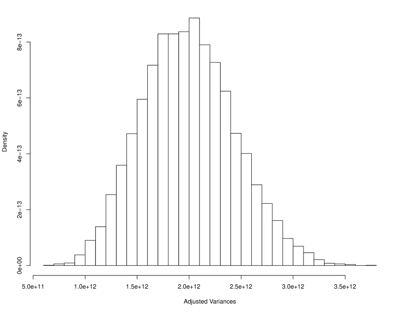
(a) Bayes linear emulator.

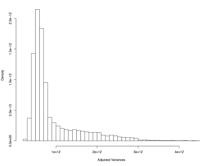
(b) Hierarchical emulator.

Figure 10: Histograms comparing the Bayes linear and hierarchical emulators adjusted variances for the ensemble mean NPV. Note that the seemingly large variances are inline with the simulated ensemble mean NPV which is of the order $5.0\text{\times}{10}^{07}$ $ to $6\text{\times}{10}^{07}$ $.

A crucial motivation for employing emulators as a surrogate to computer models is their speed of evaluation in order to enable further analyses such as decision support. Bayes linear emulation is known to be a very fast and efficient means of constructing emulators. In this application we achieve a substantial reduction in computation time with over 2000 emulator evaluations for new decision parameter settings per second using a single core of a standard desktop computer or laptop. This is juxtaposed with approximately 30 minutes per OLYMPUS model simulation, or 25 hours when using the entire ensemble. The combination of ensemble subsampling and Bayes linear emulation equates to an efficiency gain of the order of $10^{8}$.

The full hierarchical emulation process applied to the ensemble mean NPV requires for each OLYMPUS model the fitting of 48 separate emulators: 32 of the structured type; and 16 Bayes linear emulators, a total of 144 emulators over the three sub-selected OLYMPUS models. Next, these are combined to obtain emulators for the approximate and exact NPVs for each OLYMPUS model, before emulating the ensemble mean NPV, and then linking to the expected NPV. The computational performance is more modest achieving emulator evaluations at approximately 4 new decision parameter vectors per second using a single core, and is thus slower than Bayes linear emulation. However, in comparison with direct simulation from the OLYMPUS ensemble there is a considerable efficiency improvement of the order of $10^{4}$. This is sufficient for comprehensively exploring the decision parameter space. Moreover, the additional computational expense of hierarchical emulation can be justified by the reduction in emulator uncertainty. This is highly beneficial to performing an iterative decision support analysis where reducing emulator uncertainty is imperative for efficiently eliminating non-implausible regions of the decision parameter space, thus avoiding extra waves of extremely expensive simulations at locations that would have been ruled out by more accurate emulators. The additional computational cost is therefore offset versus the need for extra simulations. Such arguments are also relevant to analyses using single-stage (or one-shot) designs where fewer expensive computer model evaluations are required to achieve similar emulator accuracy across the parameter space. Both forms of emulators are easily parallelisable, thus permitting further efficiency gains.

6 Conclusion

We have presented a novel hierarchical emulation model in order to exploit known constrained and structured behaviour of simulator outputs for “grey-box” computer models in order to achieve more accurate predictions for quantities of interest. This is motivated by and applied to the TNO OLYMPUS Well Control Optimisation Challenge from the petroleum industry where the aim is to maximise the expected NPV as a function of well control decision parameters. We reconstrue this as a decision support problem where the utility function consists of a discounted sum of oil production, water injection and production, both by well and control interval. The first two simulator outputs exhibit partially known behaviour, constrained by choices of inputs and physical limits with respect to their corresponding target production and injection rate decision parameters respectively, with this structure encompassed within our emulator formulation. Application demonstrates superior accuracy versus Bayes linear emulators, whilst the slower speed of evaluation is mitigated by the need for fewer (waves of) simulations from the expensive computer model. Both factors are important for the overall aim of providing robust decision support under uncertainty. Moreover, we introduce multi-model ensemble subsampling techniques to efficiently identify a representative subset of models which collectively best characterises the expected NPV (or other output(s) of interest), whilst also providing a method for their prediction. This constitutes a novel application to the petroleum industry where multi-model ensembles are commonly used to represent geological uncertainty, greatly reducing the computational cost of our decision analysis.

The next step is to employ the presented hierarchical emulation methodology within iterative decision support, applied to the TNO OLYMPUS Well Control Optimisation Challenge, which incorporates a comprehensive and realistic uncertainty quantification to statistically link inferences for the computer model (OLYMPUS) with the corresponding real world physical system. See [31, Sec. 4.6 & 4.7] for details. In addition, further methodological development should focus on improving the hierarchical emulation framework. This may be achieved by revising the structured emulators change point estimation methods, classification and truncation, as well as via the refinement of the hierarchy uncertainty propagation. Another direction is multivariate structured emulation of the NPV constituents to assess their correlation and thus more accurately quantify the approximate NPV by ensemble member emulator variance in Section 4.3. Such further methodological developments must also be efficient so as not add to the computational burden.

The hierarchical emulation framework presented in this paper, whilst motivated by and tailored to the petroleum well control optimisation problem, is sufficiently flexible and adaptable to handle other (partially) known forms of computer model outputs and functions thereof. Opening “black-box” simulators and exploring functions of their output to investigate their behaviours is evidently beneficial, as is using domain expert prior knowledge and small carefully designed collections of simulations. Another example of emulating “grey-box” models is in known boundary emulation [44, 23]. The additional prior information can then be used guide the choice from existing emulation methods or to design novel forms which exploit known behavioural facets in order to achieve superior accuracy and enhance the usefulness of emulators for real world applications.

Appendix A Structured Emulation with Two-Sided Truncation

In this appendix we present an alternative variant of structured emulation exploiting the known simulator behaviour from Section 4.2 which uses a two-sided truncation, as presented in [31, Sec. 3.3.2]. It is unnecessary for the application to the TNO OLYMPUS Well Control Optimisation Challenge in Section 5, but is utilised in another application described in [31, Sec. 5.4.1 & 5.8.1]. In addition, we detail the truncated normal distribution equations used in both methodologies.

Estimation of the change points and extrapolation cut-offs remains as described in Sections 4.2.1 and 4.2.2 respectively, as does the physical maximum constraint discussed in 4.2.3. A lower truncation, denoted by $a_{i}$, may also be imposed, for example, to represent the constraint that the WOPT and WWIT NPV constituents within a control interval must be non-negative ($a_{i}=0$). Both constraints are utilised alongside the preliminary Bayes linear emulator in a modified classification step:

1. Slope Region: If $d_{jk,t_{i}}<b_{jk,t_{i}}$ or for the preliminary emulator $\operatorname{\mathbb{E}}_{\mathbf{F}_{i}^{\prime}}[f_{i}(\mathbf{d})]-3\sqrt{\operatorname{\mathrm{Var}}_{\mathbf{F}_{i}^{\prime}}[f_{i}(\mathbf{d})]}>d_{jk,t_{i}}\cdot\Delta t_{i}$, then collapse the emulator such that for the structured emulator $\operatorname{\mathbb{E}}_{\mathbf{F}_{i}^{\prime}}[f_{i}(\mathbf{d})]=d_{jk,t_{i}}\cdot\Delta t_{i}$ with fixed maximum absolute errors of size $\delta_{i}$.

2. Intermediate Region: As for the upper truncation version, if the preliminary emulator satisfies $\operatorname{\mathbb{E}}_{\mathbf{F}_{i}^{\prime}}[f_{i}(\mathbf{d})]-3\sqrt{\operatorname{\mathrm{Var}}_{\mathbf{F}_{i}^{\prime}}[f_{i}(\mathbf{d})]}\leq d_{jk,t_{i}}\cdot\Delta t_{i}<\operatorname{\mathbb{E}}_{\mathbf{F}_{i}^{\prime}}[f_{i}(\mathbf{d})]+3\sqrt{\operatorname{\mathrm{Var}}_{\mathbf{F}_{i}^{\prime}}[f_{i}(\mathbf{d})]}$, or if the additional criterion of $\operatorname{\mathbb{E}}_{\mathbf{F}_{i}^{\prime}}[f_{i}(\mathbf{d})]-3\sqrt{\operatorname{\mathrm{Var}}_{\mathbf{F}_{i}^{\prime}}[f_{i}(\mathbf{d})]}<a_{i}$ whilst $\operatorname{\mathbb{E}}_{\mathbf{F}_{i}^{\prime}}[f_{i}(\mathbf{d})]+3\sqrt{\operatorname{\mathrm{Var}}_{\mathbf{F}_{i}^{\prime}}[f_{i}(\mathbf{d})]}\leq d_{jk,t_{i}}\cdot\Delta t_{i}$, a truncated GP emulator is evaluated. The mean and variance are determined by Equations A.1 and A.2 respectively.

3. Plateau Region: In all other cases where $\operatorname{\mathbb{E}}_{\mathbf{F}_{i}^{\prime}}[f_{i}(\mathbf{d})]-3\sqrt{\operatorname{\mathrm{Var}}_{\mathbf{F}_{i}^{\prime}}[f_{i}(\mathbf{d})]}\geq a_{i}$ and $\operatorname{\mathbb{E}}_{\mathbf{F}_{i}^{\prime}}[f_{i}(\mathbf{d})]+3\sqrt{\operatorname{\mathrm{Var}}_{\mathbf{F}_{i}^{\prime}}[f_{i}(\mathbf{d})]}\leq d_{jk,t_{i}}\cdot\Delta t_{i}$, use the preliminary emulator .

The structured emulation methodology utilises a truncated Gaussian process (truncated GP) emulator for which the mean and variance are determined by Equations A.1 and A.2 respectively [24], where $\phi(\cdot)$ and $\Phi(\cdot)$ represent the probability density and cumulative distribution functions respectively of a standard normal distribution. These are computed assuming a preliminary Gaussian process emulator with posterior mean and variance, abbreviated to $\mu_{i}$ and $\sigma_{i}^{2}$ respectively, equal to the computed adjusted expectation and variance, and truncation bounds $a_{i}$ and $b_{i}=d_{jk,t_{i}}\cdot\Delta t_{i}$, with $\alpha_{i}=\frac{a_{i}-\mu_{i}}{\sigma_{i}}$, and $\beta_{i}=\frac{b_{i}-\mu_{i}}{\sigma_{i}}$. This form of emulation is used in the intermediate uncertain region around the change point true location.

$$\operatorname{\mathbb{E}}_{\mathbf{F}_{i}^{\prime}}[f_{i}(\mathbf{d})\mid a_{i}<f_{i}(\mathbf{d})<b_{i}] {}=\mu_{i}+\sigma\dfrac{\phi(\alpha_{i})-\phi(\beta_{i})}{\Phi(\beta_{i})-\Phi(\alpha_{i})}$$ (A.1)

$$\operatorname{\mathrm{Var}}_{\mathbf{F}_{i}^{\prime}}[f_{i}(\mathbf{d})\mid a_{i}<f_{i}(\mathbf{d})<b_{i}] {}=\sigma_{i}^{2}\left[1+\dfrac{\alpha_{i}\phi(\alpha_{i})-\beta_{i}\phi(\beta_{i})}{\Phi(\beta_{i})-\Phi(\alpha_{i})}-\left(\dfrac{\phi(\alpha_{i})-\phi(\beta_{i})}{\Phi(\beta_{i})-\Phi(\alpha_{i})}\right)^{2}\right]$$ (A.2)

Appendix B TNO OLYMPUS Well Control Optimisation Challenge – Extended Results

In this appendix we extend our discussion of results from Section 5 for the TNO OLYMPUS Well Control Optimisation Challenge (see Section 2 for an overview) using methodology proposed in Section 4.

B.1 OLYMPUS Exploratory Analysis – Additional Plots and Discussion

Our exploratory analysis identifies large differences in the absolute contributions of oil and water, both production and injection, to the NPV objective function. This feature has potential ramifications for emulation and decision support. An assessment of the absolute contributions approximated within one year intervals for the OLYMPUS 25 NPV is shown in Figure 11 using each of the 20 exploratory analysis decision parameter vectors represented by different colours. In Equation 2.3 the oil contribution (solid lines), $\lvert Q_{j,op}(\mathbf{d},t_{i})\cdot r_{op}\rvert$, is dominant versus both the absolute water production contribution (dot-dashed lines), $\lvert Q_{j,wp}(\mathbf{d},t_{i})\cdot r_{wp}\rvert$, and water injection contribution (dotted lines), $\lvert Q_{j,wi}(\mathbf{d},t_{i})\cdot r_{wi}\rvert$, as well as their sum (dashed lines), $\lvert Q_{j,wp}(\mathbf{d},t_{i})\cdot r_{wp}+Q_{j,wi}(\mathbf{d},t_{i})\cdot r_{wi}\rvert$. For earlier time intervals the magnitude of the oil contribution to the NPV is typically of the order of 100 times the combined water contribution which decays towards 10 times larger for later time intervals. Plotting on the logarithmic scale in Figure 11(b) facilitates an easier comparison of the water contributions. It is observed that water injection contributes a much larger amount to the NPV, particularly for earlier time intervals. This is to be expected since production wells are drilled within regions containing a high oil concentration, hence at initial times there should be very little water production. At later times the contribution becomes more alike as an increased quantity of water is produced in order to maintain oil production, whilst also noting the higher fixed cost per barrel of water produced versus injected. Similar observations are made for other OLYMPUS ensemble members.

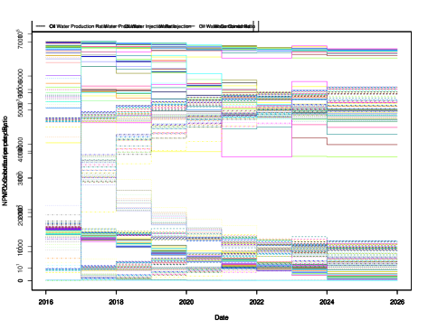
(a) Raw scale.

(b) Logarithmic scale.

Figure 11: OLYMPUS 25 approximate absolute contribution to the NPV per year for each of the exploratory simulations shown as coloured lines. The NPV is decomposed into the oil production (solid line), absolute water production (dot-dashed line) and injection (dotted line), and the total water contribution (dashed line), with each scaled by the respective fixed NPV cost parameter. These are $\lvert Q_{j,op}(\mathbf{d},t_{i})\cdot r_{op}\rvert$, $\lvert Q_{j,wp}(\mathbf{d},t_{i})\cdot r_{wp}\rvert$, $\lvert Q_{j,wi}(\mathbf{d},t_{i})\cdot r_{wi}\rvert$ and $\lvert Q_{j,wp}(\mathbf{d},t_{i})\cdot r_{wp}+Q_{j,wi}(\mathbf{d},t_{i})\cdot r_{wi}\rvert$ in Equation 2.3 respectively. The top and bottom plots are on the raw and logarithmic scale respectively.

B.2 Subsampling from Geological Multi-Model Ensembles – Additional Plots

Preliminary graphical investigations utilise plots of the ensemble mean versus the individual model over a range of outputs of interest for the wave 0 simulations. Examples of these plots are shown in Figure 12 where the black line denotes equality between the ensemble mean and individual ensemble member model output. The main outputs of interest stem from the NPV objective function and include: the ensemble mean NPV, oil production, water production and injection totals, both for the field and by well, as well as over the entire field lifetime, and for control intervals. Note that this is a preliminary graphical assessment which is limited to identifying one-dimensional relationships. Figures 12(a), 12(b) and 12(c) show strong linear relationships with fairly limited variation providing evidence that even as individual models, OLYMPUS 25, 33 & 45 are potentially representative for the ensemble mean. An appropriate (linear) transformation may be applied in the cases seen in Figures 12(b) and 12(c). In contrast OLYMPUS 50 does not appear to be a good representative model, at least individually, as seen in Figure 12(d) where the relationship is more challenging to model. This graphical investigation is also useful as a preliminary screening technique yielding a subset of 9 models to investigate further: OLYMPUS 2, 6, 11, 23, 25, 33, 35, 37, & 38.

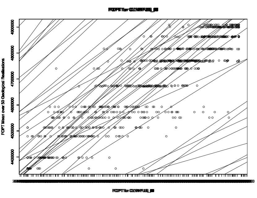
(a) OLYMPUS 25 FOPT.

(b) OLYMPUS 45 WOPTPROD2.

(c) OLYMPUS 33 FWIT.

(d) OLYMPUS 50 WOPTPROD10.

Figure 12: Subsampling from the multi-model OLYMPUS ensemble preliminary graphical investigations showing the ensemble mean versus individual model outputs. The black line denotes equality between the ensemble mean and individual model outputs.

The combination of different OLYMPUS models is assessed using the linear model subsampling technique in 4.1. This is first applied to the above proposed subset of 9 OLYMPUS models before considering all models in a both directions stepwise selection with AIC. Only $\tilde{N}=3$ models are necessary for a large number of the investigated outputs, as demonstrated in Figure 13 showing the linear model adjusted $R^{2}$ values for various outputs. All are high with most greater than 0.95 implying that the majority of the ensemble variation can be explained by a small subset. These are OLYMPUS 25, 33, & 45. It is noted that OLYMPUS 25 & 33 were identified as part of the proposed subset of models, where as OLYMPUS 45 was not. This is because for certain outputs it was judged that OLYMPUS 45 did not provide a sufficiently good representation of the ensemble mean, however, in combination with OLYMPUS 25 & 33 via the linear models, these models collectively provide a good characterisation of the ensemble mean NPV, as well as other outputs.

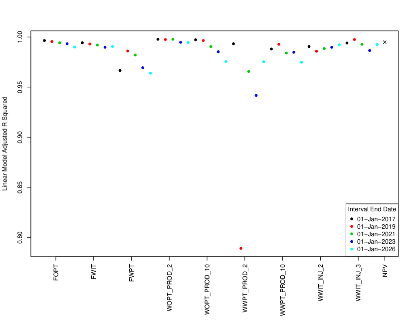
Figure 13: Adjusted $R^{2}$ values for the OLYMPUS ensemble subsampling linear models of the form in Equation 4.1 for the ensemble mean of various outputs within control intervals using the same subset of $\tilde{N}=3$ OLYMPUS models as predictors.

B.3 Targeted Bayesian Design Methodology

We employ a targeted Bayesian design algorithm in Section 5.3 to efficiently sample from the decision parameter space by incorporating prior reservoir engineering knowledge. This entails imposing: operational range constraints on the decision parameter control rates (as is standard within the computer modelling literature); and a difference constraint on time consecutive controls to avoid unphysical large temporal variation which is poor engineering practice. Consequently, the decision parameters are not mutually independent. After splitting the decision parameters into independent subgroups by well, $\mathbf{d}_{jk}\in D^{(jk)}$, the difference constraint stipulates that $\lvert d_{jk,t_{i}}-d_{jk,t_{i}-1}\rvert\leq\Delta_{i},\ i=2,\ldots,D^{(jk)}$, where $D^{(jk)}$ is the number of control intervals for well $jk$. The decision parameter space is no longer a hypercube, thus motivating the need for a Bayesian design informed by this prior information.

Our targeted Bayesian design algorithm involves a re-parameterisation and sampling the sum of the parameters and their time consecutive differences. First assume each $d_{jk,t_{i}}\in[0,1]$. Define $t=\sum_{i=1}^{D^{(jk)}}d_{jk,t_{i}}\in[0,D^{(jk)}]$ to be the sum of the parameters and $\delta_{i}=\frac{d_{jk,t_{i}}-d_{jk,t_{i}-1}}{\sqrt{2}}$ for $i=2,\dots,D^{(jk)}$, to be the scaled differences where the scaling by $\frac{1}{\sqrt{2}}$ is required due to the rotation of the parameter space in this alternative parametrisation. The new parameters are mutually orthogonal with $t\in[0,D^{(jk)}]$ and $\lvert\delta_{i}\rvert\leq\Delta_{i}^{\prime}=\frac{\Delta_{i}}{\sqrt{2}}$. This re-parametrisation is the represented by linear transformation $(t,\boldsymbol{\delta})^{\mathrm{T}}=L\mathbf{d}_{jk}$ in Equation B.1 where $L$ is the transformation matrix. Sampling in the re-parametrised space automatically satisfies the difference constraints with a sample for $\mathbf{d}_{jk}$ obtained via $\mathbf{d}_{jk}=L^{-1}(t,\boldsymbol{\delta})^{\mathrm{T}}$. The range constraints, $d_{jk,t_{i}}\in[0,1]$, must also then be verified.

$$\begin{pmatrix}t\\ \delta_{2}\\ \delta_{3}\\ \delta_{4}\\ \vdots\\ \delta_{D^{(jk)}}\end{pmatrix}=\begin{pmatrix}1&1&1&1&\cdots&1&1\\ \nicefrac{{-1}}{{\sqrt{2}}}&\nicefrac{{1}}{{\sqrt{2}}}&0&0&\cdots&0&0\\ 0&\nicefrac{{-1}}{{\sqrt{2}}}&\nicefrac{{1}}{{\sqrt{2}}}&0&\cdots&0&0\\ 0&0&\nicefrac{{-1}}{{\sqrt{2}}}&\nicefrac{{1}}{{\sqrt{2}}}&\cdots&0&0\\ \vdots&\vdots&\vdots&\vdots&\ddots&\vdots&\vdots\\ 0&0&0&0&\cdots&\nicefrac{{-1}}{{\sqrt{2}}}&\nicefrac{{1}}{{\sqrt{2}}}\end{pmatrix}\begin{pmatrix}d_{jk,1}\\ d_{jk,2}\\ d_{jk,3}\\ d_{jk,4}\\ \vdots\\ d_{jk,D^{(jk)}}\end{pmatrix}$$ (B.1)

In order to ensure good exploration along the $t$-direction, thought to be important by reservoir engineers, we propose preserving an initial sample of the parameter sums, and then uniformly resample $\boldsymbol{\delta}$ until both constraint types are satisfied. There is freedom to choose the sampling distribution of $t$ with probability density function, $f_{T}(t)$, dependent on the analysis. We use a truncated normal distribution with other examples being: uniform; mixture of uniforms; and transformed beta distributions. Orthogonal projection of the samples onto the line $d_{jk,1}=d_{jk,2}=\cdots=d_{jk,D^{(jk)}}$ will approximately follow the specified distribution.

The process of generating a sample of size $n$ for an independent subgroup of parameters is described in the rejection style Algorithm 1 yielding matrix $B$ in which each column is a sampled vector of decision parameters. If $t$ is close to 0 or $D^{(jk)}$ the rejection step can be computationally time consuming with the efficiency improved by sampling the differences conditional on $t$. This algorithm may be applied separately to each independent subgroup of decision parameters for improved efficiency before combing to obtain a design over the full decision parameter space. Design optimisation may be performed using standard design selection criteria, for example, minimax or maximin design [38], both for the designs by subgroup and the full design by combining using random permutations. Further discussion of the targeted Bayesian design method is presented in [31, Sec. 4.3].

Result: Matrix $B$ of columns of sampled parameter vectors

Let $\mathbf{t}$ be a vector of $n$ samples of $t\sim f_{T}(t)$;

Let $B$ be an empty matrix of $D^{(jk)}$ rows;

Define $dimension(\cdot)$ to be a function to obtain the length of a vector;

while $dimension(\mathbf{t})>0$ do

       foreach t in $\mathbf{t}$ do

             Set $\epsilon_{i}=\min\{t,D^{(jk)}-t,\Delta_{i}^{\prime}\}$;

             Generate $\delta_{i}\mid t\sim\mathcal{U}[-\epsilon_{i},\epsilon_{i}]$, for $i=2,\dots,D^{(jk)}$;

            

       end foreach

      Row bind $\mathbf{t},\boldsymbol{\delta}_{2},\dots,\boldsymbol{\delta}_{D^{(jk)}}$ to form matrix $B_{r,\mathrm{prop}}$;

       Compute $B_{\mathrm{prop}}=L^{-1}B_{r,\mathrm{prop}}$;

       foreach Column in $B_{\mathrm{prop}}$ do

             if Range conditions of parameter vector are satisfied then

                   Join Column to $B$;

                   Remove corresponding $t$ from $\mathbf{t}$;

                  

            else

                   Discard Column;

                  

             end if

            

       end foreach

      

end while

Algorithm 1 Sampling of parameter sums and differences preserving the initial sum of parameters sample.

B.4 Hierarchical Emulation of the Expected NPV – Additional Plots

The hierarchical emulation technique described in Section 4.2 is applied separately for each of the OLYMPUS models to the WOPT and WWIT within each control interval for wells in the CWG, with simulator outputs considered as the $f_{i}(\mathbf{d})$. Firstly, conservative estimates for the change point upper bounds are calculated from the wave 1 simulations using Equation 4.3, each time with $\delta_{i,u}=10$. This ensures numerical stability and that an upper bound is obtained with all points exceeding this definitely in the plateau region. Next the extrapolation cut-offs are estimated as the change point lower bounds, via Section 4.2.1, with $\delta_{i,l}=10$ to account for numerical precision within the simulations. The change point upper bounds and extrapolation cut-offs are illustrated for all WOPT and WWIT constituents for each wave 1 sub-selected OLYMPUS model in Figure 14 highlighting the region in which the “true” change point is believed to be situated.

(a) OLYMPUS 25 WOPT

(b) OLYMPUS 25 WWIT

(c) OLYMPUS 33 WOPT

(d) OLYMPUS 33 WWIT

(e) OLYMPUS 45 WOPT

(f) OLYMPUS 45 WWIT

Figure 14: OLYMPUS wave 1 change point upper bound and extrapolation cut-off intervals for WOPT and WWIT within each control interval with respect to their corresponding decision parameter for each of the three sub-sampled OLYMPUS models.

References

- Andrianakis and Challenor [2012] Ioannis Andrianakis and Peter G. Challenor. The effect of the nugget on Gaussian process emulators of computer models. Computational Statistics & Data Analysis, 56:4215–4228, 2012. doi: 10.1016/j.csda.2012.04.020.
- Andrianakis et al. [2015] Ioannis Andrianakis, Ian R. Vernon, Nicky McCreesh, Trevelyan J. McKinley, Jeremy E. Oakley, Rebecca N. Nsubuga, Michael Goldstein, and Richard G. White. Bayesian History Matching of Complex Infectious Disease Models Using Emulation: A Tutorial and a Case Study on HIV in Uganda. PLOS Computational Biology, 11(1), 2015. ISSN 1553-7358. doi: 10.1371/journal.pcbi.1003968.
- Andrianakis et al. [2017] Ioannis Andrianakis, Ian R. Vernon, Nicky McCreesh, Trevelyan J. McKinley, Jeremy E. Oakley, Rebecca N. Nsubuga, Michael Goldstein, and Richard G. White. History matching of a complex epidemiological model of human immunodeficiency virus transmission by using variance emulation. Journal of the Royal Statistical Society: Series C (Applied Statistics), 66(4):717–740, 2017. ISSN 0035-9254. doi: 10.1111/rssc.12198.
- Bastos and O’Hagan [2009] Leonardo S. Bastos and Anthony O’Hagan. Diagnostics for Gaussian Process Emulators. Technometrics, 51(4):425–438, 2009. doi: 10.1198/TECH.2009.08019.
- Craig et al. [1996] Peter S. Craig, Michael Goldstein, Allan H. Seheult, and James A. Smith. Bayes linear strategies for matching hydrocarbon reservoir history. In J. M. Bernardo, J. O. Berger, A. P. Dawid, and A. F. M. Smith, editors, Bayesian Statistics 5, number 5 in Proceedings of the Valencia International Meeting, pages 69–95. Clarendon Press, 1996. ISBN 978-0198523567.
- Craig et al. [1997] Peter S. Craig, Michael Goldstein, Allan H. Seheult, and James A. Smith. Pressure matching for hydrocarbon reservoirs: a case study in the use of Bayes linear strategies for large computer experiments. In Constatine Gatsonis, James S. Hodges, Robert E. Klass, Robert E. McCulloch, Peter Rossi, and Nozer D. Singpurwalla, editors, Case Studies in Bayesian Statistics, volume 121 of Lecture Notes in Statistics, pages 37–93. Springer-Verlag, 1st edition, 1997. ISBN 978-0-387-94990-1. doi: 10.1007/978-1-4612-2290-3.
- Craig et al. [1998] Peter S. Craig, Michael Goldstein, Allan H. Seheult, and James A. Smith. Constructing partial prior specifications for models of complex physical systems. Journal of the Royal Statistical Society: Series D (The Statistician), 47:37–53, 1998. ISSN 1467-9884. doi: 10.1111/1467-9884.00115.
- Craig et al. [2001] Peter S. Craig, Michael Goldstein, Jonathan C Rougier, and Allan H. Seheult. Bayesian Forecasting for Complex Systems Using Computer Simulators. Journal of the American Statistical Association, 96(454):717–729, 2001. ISSN 1537-274X. doi: 10.1198/016214501753168370.
- Cumming and Goldstein [2010] Jonathan Cumming and Michael Goldstein. Bayes Linear Uncertainty Analysis for Oil Reservoirs Based on Multisale Computer Experiments. In Anthony O’Hagan and Mike West, editors, The Oxford Handbook of Applied Bayesian Analysis, chapter 10, pages 241–270. Oxford University Press, 2010. ISBN 9780199548903.
- Edwards et al. [2019] Tamsin L. Edwards, Mark A. Brandon, Gael Durand, Neil R. Edwards, Nicholas R. Golledge, Philip B. Holden, Osabel J. Nias, Antony J. Payne, Catherine Ritz, and Andreas Wernecke. Revisiting Antarctic ice loss due to marine ice-cliff instability. Nature, 566:58–64, 2019. doi: 10.1038/s41586-019-0901-4.
- Eur [2018] EAGE/TNO Workshop on OLYMPUS Field Development Optimization, 2018. European Association of Geoscientists and Engineers (EAGE) and the Netherlands Organisation for Applied Scientific Research (TNO), EAGE Publications. ISBN 978-94-6282-261-0.
- Finetti [1974] Bruno De Finetti. Theory of Probability, volume 1. John Wiley & Sons Ltd, 1974. ISBN 978-0471201410.
- Finetti [1975] Bruno De Finetti. Theory of Probability, volume 2. John Wiley & Sons Ltd, 1975. ISBN 978-0471201427.
- Goldstein [2006a] Michael Goldstein. Bayes Linear Analysis. In Samuel Kotz, Campbell B. Read, Narayanaswamy Balakrishnan, Brani Vidakovic, and Norman L. Johnson, editors, Encyclopedia of Statistical Sciences, volume 3, pages 29–34. Wiley, 2nd edition, 2006a. ISBN 9780471150442. doi: 10.1002/0471667196.ess0986.pub2.
- Goldstein [2006b] Michael Goldstein. Subjective Bayesian Analysis: Principles and Practice. Bayesian Analysis, 1(3):403–420, 2006b. ISSN 1936-0975. doi: 10.1214/06-BA116.
- Goldstein [2011] Michael Goldstein. External Bayesian analysis for computer simulators. In J. M. Bernardo, M. J. Bayarri, J. O. Berger, A. P. Dawid, D. Heckerman, A. F. M. Smith, and M. West, editors, Bayesian Statistics 9, number 9 in Proceedings of the Valencia International Meeting, pages 201–228. Oxford University Press, 2011. ISBN 978-0199694587. doi: 10.1093/acprof:oso/9780199694587.001.0001.
- Goldstein and Rougier [2006] Michael Goldstein and Jonathan Rougier. Bayes linear calibrated prediction for complex systems. Journal of the American Statistical Association, 101(475):1132–1143, 2006. doi: 10.1198/016214506000000203.
- Goldstein and Wooff [2007] Michael Goldstein and David Wooff. Bayes Linear Statistics: Theory and Methods. Wiley Series in Probability and Statistics. Wiley, 2007. ISBN 978-0-470-01562-9. doi: 10.1002/9780470065662.
- Gramacy and Lee [2008] Robert B. Gramacy and Herbet K. H. Lee. Bayesian Treed Gaussian Process Models with an Application to Computer Modeling. Journal of the American Statistical Association, 103(483):1119–1130, 2008. ISSN 01621459. doi: 10.2307/27640148.
- Gramacy and Lee [2012] Robert B. Gramacy and Herbet K. H. Lee. Cases for the nugget in modeling computer experiments. Statistics and Computing, 22(3):713–722, 2012. doi: 10.1007/s11222-010-9224-x.
- Heitmann et al. [2009] Katrin Heitmann, David Higdon, Martin White, Salman Habib, Brian J. Williams, Earl Lawrence, and Christian Wagner. The Coyote Universe II: Cosmological Models and Precision Emulation of the Nonlinear Matter Power Spectrum. The Astrophysical Journal, 705(1):156–174, 2009. doi: 10.1088/0004-637x/705/1/156.
- Higdon et al. [2008] Dave Higdon, James Gattiker, Biran Williams, and Maria Rightley. Computer Model Calibration Using High-Dimensional Output. Journal of the American Statistical Association, 103(482):570–583, 2008. doi: 10.1198/016214507000000888.
- Jackson and Vernon [2023] Samuel E. Jackson and Ian Vernon. Efficient Emulation of Computer Models Utilising Multiple Known Boundaries of Differing Dimensions. Bayesian Analysis, 18(1):165–191, 2023. doi: 10.1214/22-BA1304.
- Johnson et al. [1994] Norman L. Johnson, Samuel Kotz, and N. Balakrishnan. Continuous Univariate Distributions, volume 1 of Wiley Series in Probability and Statistics. Wiley, 2nd edition, 1994. ISBN 9780471584957.
- Kaufman et al. [2011] Cari G. Kaufman, Derek Bingham, Salman Habib, Katrin Heitmann, and Joshua A. Frieman. Efficient emulators of computer experiments using compactly supported correlation functions, with an application to cosmology. The Annals of Applied Statistics, 5(4):2470–2492, 2011. doi: 10.1214/11-AOAS489.
- Kennedy et al. [2023] Jack C. Kennedy, Daniel A. Henderson, and Kevin J. Wilson. Multilevel emulation for stochastic computer models with application to large offshore wind farms. Journal of the Royal Statistical Society: Series C (Applied Statistics), 72(3):608–627, 2023. ISSN 0035-9254. doi: 10.1093/jrsssc/qlad023.
- Kennedy and O’Hagan [2001] Marc C. Kennedy and Anthony O’Hagan. Bayesian calibration of computer models. Journal of the Royal Statistical Society: Series B (Statistical Methodology), 63(3):425–464, 2001. doi: 10.1111/1467-9868.00294.
- Oakley [2009] Jeremy E. Oakley. Decision-Theoretic Sensitivity Analysis for Complex Computer Models. Technometrics, 51(2):121–129, 2009. ISSN 1537-2723. doi: 10.1198/TECH.2009.0014.
- Oakley and O’Hagan [2004] Jeremy E. Oakley and Anthony O’Hagan. Probabilistic sensitivity analysis of complex models: a Bayesian approach. Journal of the Royal Statistical Society: Series B (Statistical Methodology), 66(3):751–769, 2004. doi: 10.1111/j.1467-9868.2004.05304.x.
- O’Hagan et al. [1998-08-13] Anthony O’Hagan, Marc C. Kennedy, and Jeremy E. Oakley. Uncertainty Analysis and other Inference Tools for Complex Computer Codes (with discussion). In J. M. Bernardo, J. O. Berger, A. P. Dawid, and A. F. M. Smith, editors, Bayesian Statistics 6, number 6 in Proceedings of the Valencia International Meeting, pages 503–524. Clarendon Press, 1998-08-13. ISBN 978-0198523567.
- Owen [2022] Jonathan Owen. Bayesian Uncertainty Analysis and Decision Support for Complex Models of Physical Systems with Application to Production Optimisation of Subsurface Energy Resources, 2022. URL http://etheses.dur.ac.uk/14751/.
- Owen et al. [2020] Jonathan Owen, Ian Vernon, and Richard Hammersley. A Bayesian Statistical Approach to Decision Support for TNO OLYMPUS Well Control Optimisation under Uncertainty. In ECMOR XVII – 17th European Conference on the Mathematics of Oil Recovery, volume 2020. European Association of Geoscientists & Engineers (EAGE), 2020. doi: 10.3997/2214-4609.202035109.
- Pukelsheim [1994] Friedrich Pukelsheim. The Three Sigma Rule. The American Statistician, 48(2):88–91, 1994. doi: 10.2307/2684253.
- Rasmussen and Williams [2006] Carl Edward Rasmussen and Christopher K. I. Williams. Gaussian Processes for Machine Learning. The MIT Press, 2006. ISBN 0-262-18253-X. URL https://gaussianprocess.org/gpml/chapters/RW.pdf.
- Rougier et al. [2009] Jonathan Rougier, Serge Guillas, Astrid Maute, and Arthur D. Richmond. Expert Knowledge and Multivariate Emulation: The Thermosphere–Ionosphere Electrodynamics General Circulation Model (TIE-GCM). Technometrics, 51(4):414–424, 2009. doi: 10.1198/TECH.2009.07123.
- Rougier et al. [2013] Jonathan Rougier, Michael Goldstein, and Leanna House. Second-Order Exchangeability Analysis for Multimodel Ensembles. Journal of the American Statistical Association, 108(503):852–863, 2013. doi: 10.1080/01621459.2013.802963.
- Sacks et al. [1989] Jerome Sacks, William J. Welch, Toby J. Mitchell, and Henry P. Wynn. Design and Analysis of Computer Experiments. Statistical Science, 4(4), 1989. doi: doi:10.1214/ss/1177012413.
- Santner et al. [2003] Thomas J. Santner, Brian J. Williams, and William I. Notz. The Design and Analysis of Computer Experiments. Springer Series in Statistics. Springer-Verlag, 1st edition, 2003. ISBN 978-1-4419-2992-1. doi: 10.1007/978-1-4757-3799-8.
- TNO [2017] TNO. OLYMPUS Oil Reservoir Model Input Decks, 2017. URL https://www.isapp2.com/downloads/olympus-reservoir-model.pdf.
- TNO [2018] TNO. Integrated Systems Approach for Petroleum Production (ISAPP) Optimisation Challenges, 2018. URL http://www.isapp2.com/home.html.
- Vernon et al. [2010] Ian Vernon, Michael Goldstein, and Richard G. Bower. Galaxy Formation: a Bayesian Uncertainty Analysis. Bayesian Analysis, 5(4):619–670, 2010.
- Vernon et al. [2014] Ian Vernon, Michael Goldstein, and Richard Bower. Galaxy Formation: Bayesian History Matching for the Observable Universe. Statistical Science, 29(1):81–90, 2014.
- Vernon et al. [2018] Ian Vernon, Junli Liu, Michael Goldstein, James Rowe, Jen Topping, and Keith Lindsey. Bayesian uncertainty analysis for complex systems biology models: emulation, global parameter searches and evaluation of gene functions. BMC systems biology, 12, 2018. ISSN 1752-0509. doi: 10.1186/s12918-017-0484-3.
- Vernon et al. [2019] Ian Vernon, Samuel E. Jackson, and Jonathan A. Cumming. Known Boundary Emulation of Complex Computer Models. SIAM/ASA Journal on Uncertainty Quantification, 7(3):838–876, 2019. ISSN 2166-2525. doi: 10.1137/18M1164457.
- Vernon et al. [2022] Ian Vernon, Jonathan Owen, Joseph Aylett-Bullock, Carolina Cuesta-Lazaro, Jonathan Frawley, Arnau Quera-Bofarull, Aidan Sedgewick, Difu Shi, Henry Truong, Mark Turner, Joseph Walker, Tristan Caulfield, Kevin Fong, and Frank Krauss. Bayesian Emulation and History Matching of JUNE. Philosphical Transactions of the Royal Society A, 380, 2022. ISSN 1471-2962. doi: 10.1098/rsta.2022.0039.
- Vysochanskij and Petunin [1980] D. F. Vysochanskij and Y. I. Petunin. Justification of the 3- Rule for Unimodal Distribution. Theory of Probability and Mathematical Statistics, 21:25–36, 1980.
- Williamson et al. [2012] Daniel Williamson, Michael Goldstein, and Adam Blaker. Fast linked analyses for scenario-based hierarchies. Journal of the Royal Statistical Society: Series C (Applied Statistics), 61(5):665–691, 2012. ISSN 0035-9254. doi: 10.1111/j.1467-9876.2012.01042.x.
- Williamson et al. [2013] Daniel Williamson, Michael Goldstein, Lesley Allison, Adam Blaker, Peter Challenor, Laura Jackson, and Kuniko Yamazaki. History matching for exploring and reducing climate model parameter space using observations and a large perturbed physics ensemble. Climate Dynamics, 41(7):1703–1729, 2013. ISSN 1432-0894. doi: 10.1007/s00382-013-1896-4.