Highest Probability Density Conformal Regions

Abstract

We propose a new method for finding the highest predictive density set or region using signed conformal inference. The proposed method is computationally efficient, while also carrying conformal coverage guarantees. We prove that under, mild regularity conditions, the conformal prediction set is asymptotically close to its oracle counterpart. The efficacy of the method is illustrated through simulations and real applications.

Keywords: Kernel density estimation; Multimodality; Prediction; Uncertainty quantification; Signed conformal regression.

1 Introduction

Conformal prediction is a general method of creating prediction intervals that provide a non-asymptotic, distribution free coverage guarantee. Suppose we observe $n$ i.i.d. (more generally, exchangeable) copies of $((Y_{1},{\boldsymbol{X}}_{1}),(Y_{2},{\boldsymbol{X}}_{2})\ldots,(Y_{n},{\boldsymbol{X}}_{n}))$, with distribution $P$. Suppose that the first $n$ pairs are observed. Then, we want a set, $C({\boldsymbol{x}})=C_{n}((Y_{1},{\boldsymbol{X}}_{1}),$ $(Y_{2},{\boldsymbol{X}}_{2}),\ldots,$ $(Y_{n},{\boldsymbol{X}}_{n}),{\boldsymbol{x}})$ such that for a new pair $(Y_{n+1},{\boldsymbol{X}}_{n+1})$,

$$\mathbb{P}(Y_{n+1}\in C({\boldsymbol{X}}_{n+1}))\geq 1-\alpha.$$ (1)

This coverage is guaranteed unconditionally [28, 14]. If we wanted to have finite sample, distribution-free, and conditional coverage for a continuous response,

$$\mathbb{P}(Y_{n+1}\in C({\boldsymbol{X}}_{n+1})|{\boldsymbol{X}}_{n+1})\geq 1-\alpha,\quad a.s.$$ (2)

our expected prediction set length would be infinite [14].

The process for computing the prediction sets that satisfy (1) can be computationally expensive. First, the model must be retrained $n$ times, leaving out one data point each time. A non-conformity score (a measure of how unusual a prediction looks relative to the response [24], for example, the absolute difference between the response and the prediction is a non-conformity score.) is then computed on the with-held point. Only after that is done can the prediction set be computed. Oftentimes, for computational simplicity, we will train a model on the first $n_{train}$ data points, and compute the non-conformity score on the remaining $n_{cal}$ data points. This is called split conformal inference [11] or inductive conformal prediction [28]. Under some mild conditions, it was shown in [11] that the set formed using split conformal inference has the same coverage guarantees as full or classic conformal prediction.

Split conformal prediction has three steps. The first is to split the data into a training set, $Z_{tr}$, and a calibration set, $Z_{cal}$. The second step is to train a model on the training set. The model chosen depends on what non-conformity score one chooses to work with. For a continuous response, conditional mean and quantile regression models are common choices [11, 28, 22]. The third step is to compute the non-conformity scores on the calibration data. A common non-conformity score for a regression problem is the absolute difference, $V_{i}=|Y_{i}-\hat{g}({\boldsymbol{X}}_{i})|$ [18]. The prediction interval that is output will depend on the non-conformity score used, in the case of the absolute difference the interval is

$$C({\boldsymbol{X}}_{n+1})=[\hat{g}({\boldsymbol{X}}_{n+1})-Q_{1-\alpha}({\boldsymbol{V}};Z_{cal}),\hat{g}({\boldsymbol{X}}_{n+1})+Q_{1-\alpha}({\boldsymbol{V}};Z_{cal})],$$

where

$$Q_{1-\alpha}({\boldsymbol{V}};Z_{cal}):=(1-\alpha)(1+\frac{1}{|Z_{cal}|})-\text{th empirical quantile of }\{V_{i}\}.$$

and $|Z_{cal}|$ is the size of the calibration set.

A newer version of split conformal prediction is quantile conformal prediction [22, 16]. This method uses conditional quantile regression instead of conditional mean or median regression. There are a few advantages of quantile conformal prediction compared to conformal prediction for regression that uses the absolute difference non-conformity score. One such advantage is that it takes into account the model uncertainty for certain values of ${\boldsymbol{X}}$, so that not all of the prediction intervals will be of the same length [22]. There are several other non-conformity score functions given in [28, 11, 18]. The main benefit to the two shown here is that the prediction interval is easy to obtain once the non-conformity scores have been computed.

One issue that arises with the use of the non-conformity scores introduced above, is that the error rate in each tail could be anywhere from $0$ to the miscoverage rate, $\alpha$ [17, 22]. An even bigger limitation for the absolute value non-conformity score is that the intervals will necessarily be symmetric about the regression estimate [17]. We borrow from the ideas first given in [17] to adjust the tail error rates independently so that we can choose the error rate in the upper and lower tails.

Signed-conformal regression can be used to form conformal prediction intervals that guarantee specific tail error rates and (1) [17]. Define the signed error non-conformity scores, $R_{i}=Y_{i}-\hat{g}({\boldsymbol{X}}_{i})$ and $V_{i}=-1\times R_{i}$. Then the signed error conformal prediction region (SECPR) is given by

$$C({\boldsymbol{X}}_{n+1})=[\hat{g}({\boldsymbol{X}}_{n+1})-Q_{1-\alpha_{1}}({\boldsymbol{V}};Z_{cal}),\hat{g}({\boldsymbol{X}}_{n+1})+Q_{1-\alpha_{2}}({\boldsymbol{R}};Z_{cal})],$$ (3)

where

$$Q_{\delta}({\boldsymbol{V}};Z_{cal}):=(\delta)(1+\frac{1}{|Z_{cal}|})-\text{th empirical quantile of }\{V_{i}\},$$

and

$$\alpha=\alpha_{1}+\alpha_{2}.$$

For example, if one wanted a conformal prediction interval with equal tailed errors, they could take $\alpha_{1}=\alpha_{2}=\alpha/2$. Define the regression error $\epsilon:=Y-\hat{g}({\boldsymbol{X}})$. The preceding construction leverages on the observation that, for fixed $\hat{g}(\cdot)$, given any prediction set $\mathcal{C}_{\epsilon}$ for the error $\epsilon$ with coverage rate not less than $1-\alpha$, $\mathcal{C}:=\hat{g}({\boldsymbol{X}})+\mathcal{C}_{\epsilon}$ satisfies (1). The question of finding the shortest prediction set of the preceding form naturally arises. And it is well-known that the solution is unique and obtains with the $\mathcal{C}_{\epsilon}$ being the highest density region of $\epsilon$ having the same coverage rate. Below, we propose a new method for finding the highest predictive density set or region for homoskedastic errors using signed conformal regression [17]. We will briefly consider a generalization to heteroscedastic errors.

The problem of estimating upper-level or highest density sets has been widely studied [19, 6, 21, 5, 23, 15]. It involves estimating $\{z:f(z)>\lambda^{(\alpha)}\}$ for some $\lambda^{(\alpha)}>0$ and density $f$ based only on samples drawn from $f$, where $\lambda^{(\alpha)}$ is chosen such that $\int_{\{z:f(z)\leq\lambda^{(\alpha)}\}}f(y)dy=\alpha$. In Section 3, we prove that under mild conditions, our estimated set converges to this oracle set. When the assumption of homoskedasticity is violated, our method still has guaranteed coverage. Furthermore, the method can be generalized to accommodate a common form of heteroscedascity. We also compare our method via simulation to HPD-split [9]. For completeness, we include an outline of the HPD-split method in Algorithm 1.

Algorithm 1 HPD-Split

Input: level $\alpha$, data = $\mathcal{Z}=(Y_{i},{\boldsymbol{X}}_{i})_{i\in\mathcal{I}}$, test point $({\boldsymbol{x}})$, and conditional density algorithm $\mathcal{B}$
Procedure:

1:Split $\mathcal{Z}$ into a training fold $\mathcal{Z}_{tr}\overset{\Delta}{=}(Y_{i},{\boldsymbol{X}}_{i})_{i\in\mathcal{I}_{tr}}$ and a calibration fold $\mathcal{Z}_{cal}\overset{\Delta}{=}(Y_{i},{\boldsymbol{X}}_{i})_{i\in\mathcal{I}_{cal}}$

2:Fit $\hat{f}=\mathcal{B}(\{({\boldsymbol{X}}_{i},Y_{i}):i\in\mathcal{I}_{tr}\})$

3:Let $\hat{H}$ be an estimate of the cdf of the split residuals, $\hat{f}(Y|{\boldsymbol{X}})$, obtained by numerical integration

4:Let $U_{\lfloor\alpha\rfloor}$ be the $\lfloor\alpha(n_{cal}+1)\rfloor$ smallest value of $\{\hat{H}(\hat{f}(y_{i}|{\boldsymbol{x}}_{i})|{\boldsymbol{x}}_{i}):i\in\mathcal{I}_{cal}\}$

5:Build a finite grid over $\mathcal{Y}$ and, by interpolation, return $\{y:\hat{H}(\hat{f}(y|{\boldsymbol{x}})|{\boldsymbol{x}})\geq U_{\lfloor\alpha\rfloor}\}$

Existing conformal methods for finding the highest predictive density set all require computationally expensive grid searches and numerical integration [8, 9, 15]. These methods require no model for the mean or quantiles, but an estimate of the conditional density of the response given covariates. Thus, these methods are also able to capture heteroskedasticity. We show in Section 4, via simulation that our method outperforms them when homoskedastic errors is a valid assumption. Finally, a real application in Section 5 demonstrates that the proposed method compares favorably against parametric methods, even under “ideal” situation for the latter.

2 The Proposed Algorithm

We now describe our method, an extension of signed error conformal regression that estimates the highest predictive density (HPD) set called the kernel density estimator for the HPD (KDE-HPD). As with other split conformal prediction methods [11, 28], we begin by splitting our data into sets used for training and calibration. The training set is indexed by $\mathcal{I}_{tr}$ and the calibration set by $\mathcal{I}_{cal}$. Given any point estimating function, $g$, we fit $\hat{g}$ on the training set. If we are interested in having a point estimator that minimizes the squared error loss, we can use a conditional mean.

$$\hat{g}\leftarrow g(\{(Y_{i},{\boldsymbol{X}}_{i}):i\in\mathcal{I}_{tr}\})$$

Now, using the trained model, we compute non-conformity scores on the calibration set:

$$R_{k}=Y_{k}-\hat{g}({\boldsymbol{X}}_{k};\mathcal{Z}_{tr})\text{, }\forall k\in\mathcal{I}_{cal},$$

and

$$V_{k}=-1\times R_{k}.$$

Next, compute density values of the non-conformity scores, ${\boldsymbol{V}}=(V_{1},\ldots,V_{n_{cal}})^{\intercal}$, using a kernel density estimator (KDE). Denote the kernel density values as $\hat{f}(\cdot)$. The choice of which kernel to use is up to the user, as they will all perform differently depending on the true, but unknown, error distribution.

Once we’ve obtained the density values, we calculate the smallest $1-\alpha$ set with $\hat{f}(\cdot)$ and the range of ${\boldsymbol{V}}$ [4, 7]. We assume that the set is comprised of $b$ distinct intervals. Record the lower and upper endpoints of the $j-th$ interval in terms of the lower-bound quantile, ($\alpha_{j}$), and the upper-bound quantile, ($\beta_{j}$), with $j=1,\ldots,b$. Now, find $\eta_{j}({\boldsymbol{X}})=Q_{1-\alpha_{i}}({\boldsymbol{V}};Z_{cal})$ and $\gamma_{j}({\boldsymbol{X}})=Q_{1-\beta_{j}}({\boldsymbol{R}};Z_{cal})$

Now that estimates of the quantiles for the highest predictive density set have been found, we form the interval in a similar way to (3),

$$\hat{C}({\boldsymbol{x}})=\bigcup\limits_{j=1}^{b}[\hat{g}({\boldsymbol{x}};\mathcal{Z}_{tr})-\eta_{j}({\boldsymbol{x}}),\hat{g}({\boldsymbol{x}};\mathcal{Z}_{tr})+\gamma_{j}({\boldsymbol{x}})].$$

For reference, the procedure is summarized in Algorithm 2.

As long as our new data point comes from the same distribution as the first $n:=n_{cal}$ data points, $\mathbb{P}(Y_{n+1}\in\hat{C}({\boldsymbol{X}}_{n+1}))\geq 1-\alpha$. This is because our method is a version of the signed-conformal method given by [17], where we select the quantiles to attempt to minimize the length of the prediction interval.

Algorithm 2 KDE-HPD

Input: level $\alpha$, data = $\mathcal{Z}=(Y_{i},{\boldsymbol{X}}_{i})_{i\in\mathcal{I}}$, test point ${\boldsymbol{x}}$, and point estimator $g({\boldsymbol{X}};\mathcal{D})$ using $\mathcal{D}$ as data
Procedure:

1:Split $\mathcal{Z}$ into a training fold $\mathcal{Z}_{tr}\overset{\Delta}{=}(Y_{i},{\boldsymbol{X}}_{i})_{i\in\mathcal{I}_{tr}}$ and a calibration fold $\mathcal{Z}_{cal}\overset{\Delta}{=}(Y_{i},{\boldsymbol{X}}_{i})_{i\in\mathcal{I}_{cal}}$

2:Train the model $\hat{g}({\boldsymbol{x}};Z_{tr})$ using the training set

3:For each $i\in\mathcal{I}_{cal}$, compute the scores $R_{i}=Y_{i}-\hat{g}({\boldsymbol{X}}_{i};\mathcal{Z}_{tr}),\text{ and }V_{i}=-1\times R_{i},\text{ for }i\in I_{cal}$

4:Compute density values of $V_{i}$ using a kernel density estimator

5:Calculate the smallest $1-\alpha$ set which is assumed to comprise $b$ distinct intervals; record the lower and upper endpoints of the $j-th$ interval in terms of the lower-bound quantile ($\alpha_{j}$) and the upper-bound quantile ($\beta_{j}$), where j = 1, 2, …, b.

6:Find $\eta_{j}({\boldsymbol{X}})=Q_{1-\alpha_{j}}({\boldsymbol{V}};Z_{cal})$ and $\gamma_{j}({\boldsymbol{X}})=Q_{1-\beta_{j}}({\boldsymbol{R}};Z_{cal})$

Output: $\hat{C}({\boldsymbol{x}})=\bigcup\limits_{j=1}^{b}[\hat{g}({\boldsymbol{x}};\mathcal{Z}_{tr})-\eta_{j}({\boldsymbol{x}}),\hat{g}({\boldsymbol{x}};\mathcal{Z}_{tr})+\gamma_{j}({\boldsymbol{x}})]$

3 Theoretical Guarantees

Let $g(\cdot)$ be the chosen regression algorithm and $\hat{g}(\cdot)$ the corresponding point regression function estimate from the training data. Recall the regression error is $\epsilon=Y-\hat{g}({\boldsymbol{X}})$. We can also include an algorithm for heteroskedasticity, $\sigma({\boldsymbol{X}})$, for the case that the error variance varies with ${\boldsymbol{X}}$, in which case $\epsilon=(Y-\hat{g}({\boldsymbol{X}}))/\hat{\sigma}({\boldsymbol{X}})$, where $\hat{\sigma}(\cdot)$ is some heteroscedascity function estimate, obtained from the training data. For simplicity, we shall assume homoscedastic errors so that $\sigma(\cdot)=\hat{\sigma}(\cdot)\equiv 1$, unless stated otherwise. In this section we denote $n_{cal}$ as $n$.

Among the prediction regions for $Y$ of the form $\hat{g}({\boldsymbol{X}})+\mathcal{C}$ where $\mathcal{C}$ is a prediction region for $\epsilon$, of the same length and having the same (unconditional) coverage rate. For a fixed coverage rate, say $1-\alpha$, it suffices to find the shortest prediction region for $\epsilon$. It is same as the highest density region, which is generally a union of finitely many intervals. Denote the oracle region bounds as $c_{i}$, $i=1,\ldots,b$, respectively. The oracle region is then equal to $\mathcal{C}:=(c_{1},c_{2})\cup\ldots\cup(c_{b-1},c_{b})$, with $f(c_{1})=\ldots=f(c_{b})$ and the common value defined as $\lambda^{\alpha}$, which is assumed to be well-defined and a unique value. This value of $\lambda^{\alpha}$ is the cutoff such that $P(\{z:f(z)\leq\lambda^{\alpha}\})=\alpha$. Let the estimated value of $\lambda^{\alpha}$ using kernel density estimation be denoted $\hat{\lambda}^{\alpha}$. Under some assumptions, we can bound how close KDE-HPD gets to the “oracle” prediction region for $Y$ which is defined as $\hat{g}({\boldsymbol{X}})+\{z:f(z)>\lambda^{\alpha}\}$. (In the heteroscedastic case, it is given by $\hat{g}({\boldsymbol{X}})+\hat{\sigma}({\boldsymbol{X}})\times\{z:f(z)>\lambda^{\alpha}\}$.) Because we are interested in the predictive accuracy of the algorithm with fixed $\hat{g}(\cdot)$ and $\hat{\sigma}(\cdot)$, obtained by training with the training data, it suffices to first study the proximity of $\{z:f(z)>\lambda^{\alpha}\}$ to its estimate based on the kernel density estimation, in terms of their Hausdorff distance, followed by an investigation of the effects due to conformalization. The following assumptions are required for the theoretical guarantees.

Assumption 1.

$(Y_{i},{\boldsymbol{X}}_{i},i=1,\ldots,n)\overset{i.i.d.}{\sim}P.$

Let $K(z)$ be the non-negative kernel function chosen, $h$ be the bandwidth of the chosen KDE. Then, the kernel density estimate of $f(z)$ is $\hat{f}(z)=\frac{1}{nh}\sum\limits_{i=1}^{n}K(\frac{z_{i}-z}{h})$, where $z_{i}=y_{i}-\hat{g}({\boldsymbol{x}}_{i})$.

Assumption 2.

$K(z)$ is symmetric about the origin, $||K||_{\infty}=K(0)$, and $\int|K(z)|^{r}dz<\infty$ for all $r\geq 1$.

Assumption 3.

$\int\limits_{-\infty}^{\infty}K(z)dx=1$.

Assumption 4.

There exist $\rho$, $C_{\rho}$, $t_{0}>0$ such that for $|t|>t_{0}$,

$$K(t)\leq C_{\rho}exp(-t^{\rho}).$$

Assumption 5.

$||f||_{\infty}<M$, for some constant $M$.

Assumption 6.

The density $f$ is Hölder smooth of order $\eta$ for $0<\eta\leq 1$. That means that there exists constant $C_{\eta}>0$ such that $|f(z)-f(z^{\prime})|\leq C_{\eta}|z-z^{\prime}|^{\eta}$, $\forall z,z^{\prime}$.

Assumption 7.

As $n\to\infty$, the bandwidth parameter $h\to 0$ at a rate such that $\log(n)/(nh)\to 0$.

Assumption 8.

Let $0<\beta<\infty$. There exist $\lambda_{0},\lambda_{1}$, $\check{C}_{\beta}$, $\hat{C}_{\beta}$, $\psi>0$ such that $\lambda_{0}<\lambda^{\alpha}-\psi$ so that for all $\lambda^{*}\in[\lambda^{\alpha}-\psi,\lambda^{\alpha}+\psi]$, the following holds for $z\in L_{f}(\lambda_{0})\backslash L_{f}(\lambda^{*})$.

$$\check{C}_{\beta}\cdot d(z,L_{f}(\lambda^{*}))^{\beta}\leq\lambda^{*}-f(z)\leq\hat{C}_{\beta}\cdot d(z,L_{f}(\lambda^{*}))^{\beta},$$

where $L_{f}(\lambda^{*}):=\{z:f(z)>\lambda^{*}\}$, $d(z,A):=\inf_{z^{\prime}\in A}\{|z-z^{\prime}|\}$, $\hat{C}_{\beta}$ and $\check{C}_{\beta}$ are constants. Moreover, $L_{f}(\lambda_{0})$ has finite Lebesgue measure.

Assumption 9.

The density function $f$ satisfies the $\gamma-$exponent at level $\lambda^{\alpha}$, i.e., there exist constants $\tau_{0}>0$ and $b_{1},b_{2}>0$, such that

$$b_{1}|\tau|^{\gamma}\leq|P(\{z:f(z)\leq\lambda^{\alpha}+\tau\})-\alpha|\leq b_{2}|\tau|^{\gamma},\>\forall\>-\tau_{0}\leq\tau\leq\tau_{0}.$$

Remark: Assumptions 2–4 are mild regularity conditions on the kernel function. Assumptions 5 and 6 are general smoothness conditions satisfied by commonly used density functions. Assumption 7 imposes conditions on the bandwidth commonly used in the literature. Assumption 8 is similar to a condition in [10]. Assumption 9 was first introduced by [19], and was later used in many other papers on density estimation [21, 25, 12]. This assumption and assumption 6 cannot hold at the same time unless $\gamma(\eta\wedge 1)\leq 1$ [1, 13]. This will always be true when $\gamma=1$. The condition is a requirement that the density is not flat at $\lambda^{\alpha}$ (for stability), nor steep (for accurately selecting $\hat{\lambda}^{\alpha}$) [13].

We follow [10, 5] in bounding the Hausdorff distance between two upper-level density sets. The difference in our approach is that we look to bound the distance between the true density and true cutoff with an estimated density and estimated cutoff instead of an estimated density and known cutoff. The proof of the following result is deferred to the Appendix.

Theorem 1.

Assume the validity of assumptions 1 - 9, with $\eta=1$ in assumption 6, and $\gamma=1$ in assumption 9. Suppose the bandwidth $h>\log(n)/n$. Then there exists a constant $C$ such that for $n$ sufficiently large, the following holds with probability at least $1-O(1/n)$.

$$d_{H}(\{z:\hat{f}(z)>\hat{\lambda}^{\alpha}\},\{z:f(z)>\lambda^{\alpha}\})<C\left(h+\sqrt{\frac{\log n}{nh}}\right),$$

where $\beta$ is as in assumption 9, $d_{H}$ is the Hausdorff distance, $d_{H}(A,B)=\max\{\sup\limits_{z\in A}d(z,B),\sup\limits_{y\in B}d(y,A)\}$, and $f(z)$ is the probability density function for $\epsilon=Y-\hat{g}({\boldsymbol{X}})$. Here we define $d(z,A)=\inf\limits_{y\in A}\{|z-y|\}$.

Remark: Taking $h=n^{-1/3}$ optimizes the above result, but the result still holds when taking $h=n^{-1/5}$, which is the rate used to minimize the mean integrated squared error of a kernel density estimator. This allows the easy use of existing kernel density estimation packages.

In other words, the probability of picking a prediction set that is very different from the oracle prediction set is small, and goes to zero as the sample size of our calibration set becomes large.

Theorem 1 implies that the set output by KDE-HPD is asymptotically close to the oracle set, as $n\to\infty$. To see this, for simplicity, we look at one cutoff point from the error term. Denote this cutoff point as $\tau_{1}$. Let $\alpha_{1}$ be the empirical CDF value for $\epsilon_{1}$. By the Glivenko–Cantelli theorem we know that this will converge to the true CDF value of $\tau_{1}$. Now, the conformal adjustment quantile is the empirical quantile of $\frac{\alpha_{1}(n+1)}{n}$. Clearly this goes to $\alpha_{1}$ as $n\to\infty$. Finally, assume that the quantile function of $\epsilon$ is continuous. By [27, Lemma 21.2], the empirical quantile will converge to the true quantile. So, for a large sample size the set output by KDE-HPD should be close to the oracle set. The benefit of this conformal adjustment is that when we have a small or medium sample size, we have conformal coverage guarantees.

4 Simulation Studies

In this section, we demonstrate our performance compared to that of HPD-split from [9] in four different scenarios. Each simulation scenario was run $1,000$ times with $1,000$ observed data points, 50 data points that were used for out of sample prediction, and a goal of $1-\alpha=0.90$ coverage. One predictor was generated, $X\sim\text{Unif}(-5,5)$. We used the default settings for HPD-split. For our method, we used 50% of the data in the training set and 50% of the data in the calibration set. We correctly specified the conditional mean and estimated the coefficients using linear regression. In the bowtie simulation scenario, we included a model for heteroskedasticity. We used 25% of the data to train the conditional mean model, 25% were to train $\hat{\sigma}(X)$, a random forest model with a response of $|Y-\hat{g}({X})|$, and 50% in the calibration set. In all simulations we used a Normal kernel with default bandwidth selection in R. We compared the coverage, average size, and average run-time for the entire simulation to run in seconds. The computer used to run the simulations has a 12th Gen Intel i9-12900K with 16 cores up to 5.2GHz and 32GB of memory. All simulations were run using R Statistical Software version 4.3.1 [20]. Simulation standard errors are given in parenthesis. The simulation setups are below. Results can be found in Tables 1 - 5.

• Unimodal and symmetric: $Y|X\sim\mathcal{N}(5+2X,1)$

• Unimodal and skewed: $Y|X=5+2X+\epsilon$, $\epsilon\sim\text{Gamma}(\text{Shape}=7.5,\text{Rate}=1)$

• Bimodal: $Y|X=5+2X+\epsilon$, $\epsilon\sim p\mathcal{N}(-6,1)+(1-p)(\text{Gamma}(\text{Shape}=2,\text{Rate}=1/2)+2)$, and $p\sim\text{Bernoulli}(0.5)$

• Heteroskedastic: $Y|X=5+2X+\epsilon|X$, $\epsilon|X\sim\text{Gamma}(\text{Shape}=1+2|X|,\text{Rate}=1+2|X|)$

• Bowtie: $Y|X=5+2X+\epsilon|X$, $\epsilon|X\sim\mathcal{N}(0,|X|)$, where $|X|$ is the standard deviation of the Normal distribution.

Approach	Coverage	Length	Computation Time
HPD-split	0.892 (0.001)	3.876(0.011)	19.85
KDE-HPD	0.902 (0.001)	3.323 (0.004)	0.002

Table 1: Unimodal and Symmetric

Figure 1: Comparison of Lengths for Unimodal and Symmetric

Approach	Coverage	Length	Computation Time
HPD-split	0.897 (0.001)	10.559(0.022)	20.10
KDE-HPD	0.899 (0.001)	10.021 (0.027)	0.002

Table 2: Unimodal and Skewed

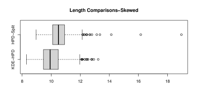
Figure 2: Comparison of Lengths for Unimodal and Skewed

Approach	Coverage	Length	Computation Time
HPD-split	0.913 (0.002)	36.524(0.506)	19.33
KDE-HPD	0.899 (0.001)	24.302 (0.103)	0.003

Table 3: Bimodal

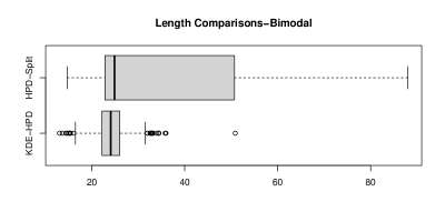
Figure 3: Comparison of Lengths for Bimodal

Approach	Coverage	Length	Computation Time
HPD-split	0.894 (0.001)	1.717 (0.005)	20.10
KDE-HPD	0.900 (0.001)	1.784 (0.007)	0.003

Table 4: Heteroskedastic

Figure 4: Comparison of Lengths for Heteroskedastic

Approach	Coverage	Length	Computation Time
HPD-split	0.920 (0.001)	16.783 (0.023)	19.01
KDE-HPD	0.898 (0.001)	10.872 (0.007)	0.024

Table 5: Bowtie

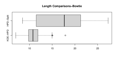
Figure 5: Comparison of Lengths for Bowtie

A visual comparison of the lengths can be found in Figures 1 - 5. Examples of the KDE-HPD prediction regions can be found in Figures 6 - 10. Examples of HPD-split prediction regions can be found in Figures 11 - 15. We can see from the simulation results that not only is KDE-HPD much faster than HPD-split, it also performs better in nearly all of the scenariors. HPD-split also gives irregular shaped prediction regions because it is fitting very closely to the observed data. For example, see Figure 11 and Figure 12. We can see in Figure 10 that KDE-HPD does very well with heteroskedastic errors as long as a model for them is included. Compared to Figure 15, KDE-HPD is much more adaptive to the changes in variability in the conditional response. The speed difference may seem small, but if one decided to use the Jackknife+ or CV+ [2], the computation time for HPD-split would quickly add up.

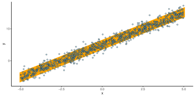
Figure 6: Prediction Regions KDE-HPD: Unimodal and Symmetric. The orange shaded region is the prediction set from one simulation.

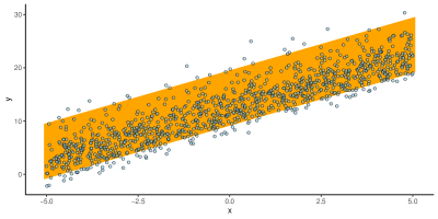
Figure 7: Prediction Regions KDE-HPD: Unimodal and Skewed. The orange shaded region is the prediction set from one simulation.

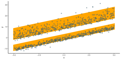
Figure 8: Prediction Regions KDE-HPD: Bimodal. The orange shaded region is the prediction set from one simulation.

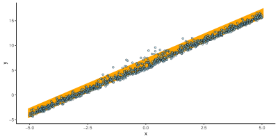
Figure 9: Prediction Regions KDE-HPD: Heteroskedastic. The orange shaded region is the prediction set from one simulation.

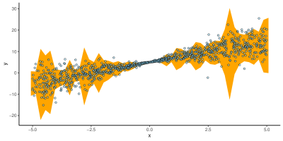
Figure 10: Prediction Regions KDE-HPD: Bowtie. The orange shaded region is the prediction set from one simulation.

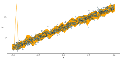
Figure 11: Prediction Regions HPD-split: Unimodal and Symmetric. The orange shaded region is the prediction set from one simulation.

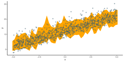
Figure 12: Prediction Regions HPD-split: Unimodal and Skewed. The orange shaded region is the prediction set from one simulation.

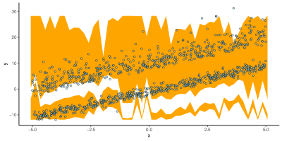
Figure 13: Prediction Regions HPD-split: Bimodal. The orange shaded region is the prediction set from one simulation.

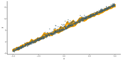
Figure 14: Prediction Regions HPD-split: Heteroskedastic. The orange shaded region is the prediction set from one simulation.

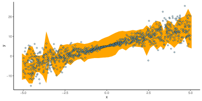
Figure 15: Prediction Regions HPD-split: Bowtie. The orange shaded region is the prediction set from one simulation.

5 Real Data Analysis

All analyses were performed using R Statistical Software [20]. We compare KDE-HPD with Normal parametric prediction intervals on a portion of the NHANES 2005-2006 data set with height, weight, and gender of individuals [26]. For both KDE-HPD and the Normal parametric prediction intervals, a linear regression model was used where the covariates were gender and weight and the response was height. We can see in Figure 16 that the residuals from this model are fairly homoskedastic. There were 5,107 observations in the data set. For KDE-HPD, 2,000 were used for training, 2,000 were used for calibration, and 1,107 were used for out of sample prediction. For the parametric approach, 4,000 were used for training the model and 1,107 were used for out of sample prediction. The data were randomly permuted 2,000 times. The average coverage, conditional coverage on gender, and average length are given in Table 6.

Figure 16: Residuals from a linear regression vs a subject’s weight

Approach	Coverage	Coverage (Male)	Coverage (Female)	Length
KDE-HPD	0.899	0.886	0.911	8.932
Parametric	0.903	0.889	0.916	8.995

Table 6: NHANES Comparison 1

Slight heteroskedasticity can be seen for individuals who weigh more than 280 pounds in Figure 16, so we looked at a second comparison that included a model for the heteroskedasticity for KDE-HPD to attempt to improve the conditional coverage. In this case, 1,000 observations were used to train the conditional mean model, 1,000 observations were used to train the model for heteroskedasticity (a linear model where the response was $|Y_{i}-\hat{g}({\boldsymbol{X}}_{i}|$ and the covariates were weight and gender), 2,000 observations were used in the calibration set, and 1,107 observations were used for out of sample prediction. The Normal parametric approach was the same as the first scenario. The results can be found in Table 7. Adding this model slightly improves the conditional coverage without increasing the interval lengths very much.

Approach	Coverage	Coverage (Male)	Coverage (Female)	Length
KDE-HPD	0.899	0.889	0.909	8.978
Parametric	0.903	0.889	0.916	8.995

Table 7: NHANES Comparison 2

A linear regression of weight vs height is often used in introductory classes as a realistic example of linear regression with Normal errors. Looking at this application in both scenarios, we can see the prediction sets output by KDE-HPD have slightly smaller lengths than the Normal parametric prediction intervals, showing that KDE-HPD can give similar results to other methods when their ideal conditions are met. Adding a second model to help with the slight heteroskedasticity for KDE-HPD slightly improves the conditional coverage without sacrificing the length. It’s clear that when we use good models with KDE-HPD, the results are very good.

A second real data analysis was performed to compare KDE-HPD with HPD-split on a data set that included the price, square footage, and air conditioning status of homes [3]. We can see in Figure 17, the residuals are clearly heteroskedastic. The data were randomly permuted 200 times. There were 521 observations, in each permutation for KDE-HPD 60 observations were used to train a linear regression for the conditional mean of the selling price, 140 were used to train a random forest for the heteroskedastic model, $\hat{\sigma}=|\text{Price}-\hat{g}({\boldsymbol{X}})|$, 100 for calibration, and 221 for out of sample prediction. For HPD-split, 200 observations were used to train the model, 100 were used for conformal calibration, and 221 were used for out of sample prediction. The average coverage, conditional coverage on AC, and average length are given in Table 8.

Figure 17: Residuals from a linear regression vs a home’s square footage

Approach	Coverage	Coverage (AC)	Coverage (no AC)	Length
HPD-Split	0.886	0.893	0.851	274.353
KDE-HPD	0.886	0.888	0.877	260.201

Table 8: Housing Comparison

Not only does KDE-HPD have a smaller average length while maintaing the same coverage, it also has better conditional coverage than HPD-split. HPD-split undercovers the selling price of homes without AC (about 17% of the data), leading to unbalanced coverage. In both real data scenarios, it is clear that KDE-HPD is adaptable to commonly found errors terms, computationally efficient, and easy to implement. It also significantly outperforms other methods.

6 Acknowledgments

Max Sampson was partially funded by National Institutes of Health Predoctoral Training Grant T32 HL 144461.

APPENDIX: Proof of Theorem 1

Proof.

First, we will derive an upper bound for $|\lambda^{\alpha}-\hat{\lambda}^{\alpha}|$. [13, Theorem 3.3] derived a related bound but they defined $\hat{\lambda}^{\alpha}$ in terms of certain quantile of the kernel density estimate at the observed data which is different from our definition as the cutoff of an upper kernel density set, hence different proof techniques are required. Our proof leverages the recent result of [10, Theorem 2] on the uniform convergence of the kernel density estimate to the true density, specifically, under assumptions 1–6, it holds that with probability at least $1-1/n$, uniformly in $h>(\log n/n)$,

$$\sup_{z\in R}|\hat{f}(z)-f(z)|<C\left(h+\sqrt{\frac{\log n}{nh}}\right):=c_{n},$$ (4)

where $n$ is the training sample size. On the event $\mathcal{E}_{n}$ when the preceding uniform convergence holds, it is readily shown that, for any $t$,

$$\{z:f(z)\leq t-c_{n}\}\subseteq\{z:\hat{f}(z)\leq t\}\subseteq\{z:f(z)\leq t+c_{n}\}.$$ (5)

Hence,

$$\int_{\{z:\hat{f}(z)\leq t\}}\hat{f}(z)dz$$ (6)

$$\leq \int_{\{z:f(z)\leq t+c_{n}\}}f(z)dz+\int_{\{z:f(z)\leq t+c_{n}\}}\hat{f}(z)-f(z)dz$$

$$\leq \int_{\{z:f(z)\leq t+c_{n}\}}f(z)dz+\int_{\{z:f(z)>t+c_{n}\}}f(z)-\hat{f}(z)dz$$

$$\leq \int_{\{z:f(z)\leq t+c_{n}\}}f(z)dz+c_{n}\times L(t+c_{n})$$

where $L(t)$ is the Lebesgue measure of the set $\{z:f(z)>t\}$. Similarly, on $\mathcal{E}_{n}$, we have

$$\int_{\{z:\hat{f}(z)\leq t\}}\hat{f}(z)dz$$ (7)

$$\geq \int_{\{z:f(z)\leq t-c_{n}\}}f(z)dz-c_{n}\times L(t-c_{n}).$$

Let $C_{1}>1$ be a constant to be determined. It follows from assumption 9 and inequalities (6) and (7) that for all $n$ sufficiently large,

$$\int_{\{z:\hat{f}(z)\leq\lambda^{\alpha}+C_{1}c_{n}\}}\hat{f}(z)dz\geq\alpha+b_{1}\times(C_{1}-1)\times c_{n}-c_{n}\times L(\lambda^{\alpha}+(C_{1}-1)\times c_{n}).$$ (8)

Similarly, we have

$$\int_{\{z:\hat{f}(z)\leq\lambda^{\alpha}-C_{1}c_{n}\}}\hat{f}(z)dz\leq\alpha-b_{1}\times(C_{1}-1)\times c_{n}+c_{n}\times L(\lambda^{\alpha}-(C_{1}-1)\times c_{n}).$$ (9)

Since $L(\cdot)$ is a decreasing function, for $n$ sufficiently large, $L(\lambda^{\alpha}-(C_{1}-1)\times c_{n})<L(\lambda_{0})$ which is a finite number by assumption. By choosing $C_{1}$ such that $b_{1}(C_{1}-1)>2L(\lambda_{0})$, the preceding two inequalities show that $\int_{\{z:\hat{f}(z)\leq\lambda^{\alpha}+C_{1}c_{n}\}}\hat{f}(z)dz>\alpha$ while $\int_{\{z:\hat{f}(z)\leq\lambda^{\alpha}-C_{1}c_{n}\}}\hat{f}(z)dz<\alpha$, thereby on $\mathcal{E}_{n}$, for $n$ sufficiently large, $|\hat{\lambda}^{\alpha}-\lambda^{\alpha}|<C_{1}c_{n}$; furthermore, (5) entails that

$$\mathcal{Z}_{1}:=\{z:f(z)>\lambda^{\alpha}+(C_{1}+1)c_{n}\}\subseteq\{z:\hat{f}(z)>\hat{\lambda}^{\alpha}\}\subseteq\{z:f(z)>\lambda^{\alpha}-(C_{1}+1)c_{n}\}:=\mathcal{Z}_{2}.$$

Now

$$d_{H}(\{z:\hat{f}(z)>\hat{\lambda}^{\alpha}\},\{z:f(z)>\lambda^{\alpha}\})$$

$$\leq d_{H}(\{z:\hat{f}(z)>\hat{\lambda}^{\alpha}\},\mathcal{Z}_{1})+d_{H}(\mathcal{Z}_{1},\{z:f(z)>\lambda^{\alpha}\})$$

$$\leq d_{H}(\mathcal{Z}_{2},\mathcal{Z}_{1})+d_{H}(\mathcal{Z}_{1},\{z:f(z)>\lambda^{\alpha}\})$$

$$\leq (2(C_{1}+1)c_{n}/\check{C}_{\beta})^{1/\beta}+((C_{1}+1)c_{n}/\check{C}_{\beta})^{1/\beta},$$

owing to assumption 8. Thus, on the event $\mathcal{E}_{n}$ and for $n$ sufficiently large, $d_{H}(\{z:\hat{f}(z)>\hat{\lambda}^{\alpha}\},\{z:f(z)>\lambda^{\alpha}\})$ is bounded by some fixed multiple of $c_{n}^{1/\beta}$. This completes the proof. ∎

Appendix A References

References

- [1] Jean-Yves Audibert and Alexandre B. Tsybakov “Fast Learning Rates for Plug-In Classifiers” In The Annals of Statistics 35.2 Institute of Mathematical Statistics, 2007, pp. 608–633 URL: http://www.jstor.org/stable/25463570
- [2] Rina Foygel Barber, Emmanuel J. Candès, Aaditya Ramdas and Ryan J. Tibshirani “Predictive inference with the jackknife+” In The Annals of Statistics 49.1 Institute of Mathematical Statistics, 2021, pp. 486–507 DOI: 10.1214/20-AOS1965
- [3] E. Belsley D.A. and R.E. Welsch “Regression Diagnostics. Identifying Influential Data and Sources of Collinearity” New York: Wiley, 1980
- [4] MingHui Chen and QiMan Shao “Monte Carlo Estimation of Bayesian Credible and HPD Intervals” In Journal of Computational and Graphical Statistics 8.1 [American Statistical Association, Taylor & Francis, Ltd., Institute of Mathematical Statistics, Interface Foundation of America], 1999, pp. 69–92 URL: http://www.jstor.org/stable/1390921
- [5] YenChi Chen, Christopher R. Genovese and Larry Wasserman “Density Level Sets: Asymptotics, Inference, and Visualization” In Journal of the American Statistical Association 112.520 Taylor & Francis, 2017, pp. 1684–1696 DOI: 10.1080/01621459.2016.1228536
- [6] Antonio Cuevas and Ricardo Fraiman “A Plug-in Approach to Support Estimation” In The Annals of Statistics 25.6 Institute of Mathematical Statistics, 1997, pp. 2300–2312 URL: http://www.jstor.org/stable/2959033
- [7] Rob J. Hyndman, David M. Bashtannyk and Gary K. Grunwald “Estimating and Visualizing Conditional Densities” In Journal of Computational and Graphical Statistics 5.4 [American Statistical Association, Taylor & Francis, Ltd., Institute of Mathematical Statistics, Interface Foundation of America], 1996, pp. 315–336 URL: http://www.jstor.org/stable/1390887
- [8] Rafael Izbicki, Gilson Shimizu and Rafael Stern “Flexible distribution-free conditional predictive bands using density estimators” In Proceedings of the Twenty Third International Conference on Artificial Intelligence and Statistics 108, Proceedings of Machine Learning Research PMLR, 2020, pp. 3068–3077 URL: https://proceedings.mlr.press/v108/izbicki20a.html
- [9] Rafael Izbicki, Gilson Shimizu and Rafael B. Stern “CD-split and HPD-split: Efficient Conformal Regions in High Dimensions” In Journal of Machine Learning Research 23.87, 2022, pp. 1–32 URL: http://jmlr.org/papers/v23/20-797.html
- [10] Heinrich Jiang “Uniform Convergence Rates for Kernel Density Estimation” In Proceedings of the 34th International Conference on Machine Learning 70, Proceedings of Machine Learning Research PMLR, 2017, pp. 1694–1703 URL: https://proceedings.mlr.press/v70/jiang17b.html
- [11] Jing Lei et al. “Distribution-Free Predictive Inference for Regression” In Journal of the American Statistical Association 113.523 Taylor & Francis, 2018, pp. 1094–1111 DOI: 10.1080/01621459.2017.1307116
- [12] Jing Lei, James Robins and Larry Wasserman “Efficient Nonparametric Conformal Prediction Regions”, 2011 arXiv:1111.1418 [math.ST]
- [13] Jing Lei, James Robins and Larry Wasserman “Distribution-Free Prediction Sets” PMID: 25237208 In Journal of the American Statistical Association 108.501 Taylor & Francis, 2013, pp. 278–287 DOI: 10.1080/01621459.2012.751873
- [14] Jing Lei and Larry Wasserman “Distribution Free Prediction Bands” arXiv, 2012 DOI: 10.48550/ARXIV.1203.5422
- [15] Jing Lei and Larry Wasserman “Distribution-free prediction bands for non-parametric regression” In Journal of the Royal Statistical Society Series B 76.1, 2014, pp. 71–96 URL: https://ideas.repec.org/a/bla/jorssb/v76y2014i1p71-96.html
- [16] Lihua Lei and Emmanuel J. Candès “Conformal Inference of Counterfactuals and Individual Treatment Effects” In Journal of the Royal Statistical Society Series B: Statistical Methodology 83.5, 2021, pp. 911–938 DOI: 10.1111/rssb.12445
- [17] Henrik Linusson, Ulf Johansson and Tuve Löfström “Signed-Error Conformal Regression” In Advances in Knowledge Discovery and Data Mining Cham: Springer International Publishing, 2014, pp. 224–236
- [18] Harris Papadopoulos, Kostas Proedrou, Volodya Vovk and Alex Gammerman “Inductive Confidence Machines for Regression” In Machine Learning: ECML 2002 Berlin, Heidelberg: Springer Berlin Heidelberg, 2002, pp. 345–356
- [19] Wolfgang Polonik “Measuring Mass Concentrations and Estimating Density Contour Clusters-An Excess Mass Approach” In The Annals of Statistics 23.3 Institute of Mathematical Statistics, 1995, pp. 855–881 DOI: 10.1214/aos/1176324626
- [20] R Core Team “R: A Language and Environment for Statistical Computing”, 2023 R Foundation for Statistical Computing URL: https://www.R-project.org/
- [21] Philippe Rigollet and Régis Vert “Optimal rates for plug-in estimators of density level sets” In Bernoulli 15.4 Bernoulli Society for Mathematical StatisticsProbability, 2009 DOI: 10.3150/09-bej184
- [22] Yaniv Romano, Evan Patterson and Emmanuel Candes “Conformalized Quantile Regression” In Advances in Neural Information Processing Systems 32 Curran Associates, Inc., 2019 URL: https://proceedings.neurips.cc/paper_files/paper/2019/file/5103c3584b063c431bd1268e9b5e76fb-Paper.pdf
- [23] R.. Samworth and M.. Wand “Asymptotics and optimal bandwidth selection for highest density region estimation” In The Annals of Statistics 38.3 Institute of Mathematical Statistics, 2010 DOI: 10.1214/09-aos766
- [24] Glenn Shafer and Vladimir Vovk “A Tutorial on Conformal Prediction” In Journal of Machine Learning Research 9.12, 2008, pp. 371–421 URL: http://jmlr.org/papers/v9/shafer08a.html
- [25] A.. Tsybakov “On nonparametric estimation of density level sets” In The Annals of Statistics 25.3 Institute of Mathematical Statistics, 1997, pp. 948–969 DOI: 10.1214/aos/1069362732
- [26] United States Department of Health and Human Services. Centers for Disease Control and Prevention. National Center for Health Statistics “National Health and Nutrition Examination Survey (NHANES), 2005-2006” Inter-university Consortium for PoliticalSocial Research [distributor], 2012
- [27] A.W. Van Der Vaart “Asymptotic Statistics”, Cambridge Series in Statistical and Probabilistic Mathematics, 3 Cambridge University Press, 1998 URL: https://books.google.com/books?id=udhfQgAACAAJ
- [28] Vladimir Vovk, Alex Gammerman and Glenn Shafer “Algorithmic Learning in a Random World” Berlin, Heidelberg: Springer-Verlag, 2005