Beyond the Mean: Differentially Private Prototypes for Private Transfer Learning

Abstract

Machine learning (ML) models have been shown to leak private information from their training datasets. Differential Privacy (DP), typically implemented through the differential private stochastic gradient descent algorithm (DP-SGD), has become the standard solution to bound leakage from the models. Despite recent improvements, DP-SGD-based approaches for private learning still usually struggle in the high privacy ($\varepsilon\leq 1)$ and low data regimes, and when the private training datasets are imbalanced. To overcome these limitations, we propose Differentially Private Prototype Learning (DPPL) as a new paradigm for private transfer learning. DPPL leverages publicly pre-trained encoders to extract features from private data and generates DP prototypes that represent each private class in the embedding space and can be publicly released for inference. Since our DP prototypes can be obtained from only a few private training data points and without iterative noise addition, they offer high-utility predictions and strong privacy guarantees even under the notion of pure DP. We additionally show that privacy-utility trade-offs can be further improved when leveraging the public data beyond pre-training of the encoder: in particular, we can privately sample our DP prototypes from the publicly available data points used to train the encoder. Our experimental evaluation with four state-of-the-art encoders, four vision datasets, and under different data and imbalancedness regimes demonstrate DPPL’s high performance under strong privacy guarantees in challenging private learning setups.

1 Introduction

Machine learning (ML) models are known to leak private information about their training datasets [15, 31, 66]. As a solution to provably upper-bound privacy leakage, differential privacy (DP) [28] has emerged as the de-facto standard for private training. It is usually implemented in ML through the differential private stochastic gradient descent (DP-SGD) algorithm which bounds the contribution of each data point during training and iteratively injects controlled amounts of noise [1]. Thereby, DP-SGD has been shown to increase training time and decrease the final model’s utility.

While, over the last years, there has been significant progress in improving both computational efficiency [10, 35, 47, 45, 71] and privacy-utility trade-offs [11, 21], there are a few relevant setups where DP training still yields unfavorable results. These include the high privacy regime (expressed in DP with small values of the privacy parameter $\varepsilon$, such as $\varepsilon\leq 1$), the low data regime, i.e., when only a few private data points are available for training, and when the training dataset is imbalanced, i.e., when some classes have significantly more data points than others [12, 50, 63].

There are various reasons why DP training is challenging in these setups [30, 29]. One of these is that DP protects small sets of examples due to its “group privacy” property, providing a provable bound on how much a DP algorithm can learn from small data [30]. Beyond this concern, the iterative noise addition weakens the signal from the training data, especially when only a few training data points are available. Moreover, standard approaches for learning in imbalanced setups, such as changing the sampling [23, 44, 41, 46, 49, 80], generating synthetic data for the minority classes [18], or weighing the training loss [14] are not directly compatible with DP or incur additional privacy costs. In a similar vein, each training iteration with DP training incurs additional privacy costs [1], making it hard to keep $\varepsilon$ low, i.e., to stay in the high privacy regime.

Figure 1: Overview of DPPL. We split the private data $\mathbf{X}$ per class $c$ into $\mathbf{X}_{c}$’s, infer them through a publicly pre-trained encoder, and estimate per-class prototypes $\mathbf{p}_{c}$ in the embedding space with DP. Classification of new samples $\mathbf{x}$ is performed by returning the label of the closest prototype $\mathbf{p}_{c}$ in the embedding space according to some distance function $d(\cdot,\cdot)$.

To address all of these challenges, we propose Differentially Private Prototype Learning (DPPL), a novel approach for private learning that combines prototypical networks [68], a standard algorithm for non-private few shot learning, with recent advances in training high-performance private models with DP that leverage powerful encoder models pre-trained on public data [16, 37, 62] combined with private transfer learning [47, 79, 34, 73, 32, 39, 38, 48, 54]. The main idea of our DPPL is to use the encoder as a feature extractor for the private data and to generate DP prototypes in the embedding space for each private class. To classify new data points, we then simply have to infer these points through the encoder and to return the label of the closest prototype.

Relying on DP prototypes for private learning offers significant advantages over iterative private training or fine-tuning. First, our prototypes do not require iterative noise addition. This enables to obtain less noisy predictions at lower privacy costs and improves privacy-utility trade-offs in the high privacy regime. Second, the prototypes are inherently balanced, i.e., it is possible to obtain good prototypes also at the low data regime or for underrepresented classes from imbalanced private training datasets. Third, DP prototypes are fast to obtain, enable fast inference, and, due to the DP post-processing guarantees—which express that no query to them will incur additional privacy costs—can be publicly released for performing predictions.

We propose multiple algorithms for obtaining DP prototypes, and find that prior approaches for training models with DP do not yet leverage the full capacity of the public data [47, 79, 54]: these prior approaches use the public data only for pre-training the encoder. Yet, we make the observation that we can leverage the public data additionally during the transfer learning step. By privately selecting per-class private prototypes from the public data, we can significantly decrease the privacy costs of our prototypes (even under the strong notion of pure DP, i.e., $\varepsilon$-DP) and further improve privacy-utility trade-offs.

By performing thorough experimentation with four state-of-the-art encoders and four standard vision datasets, we show that DPPL provides strong utility in the high privacy regimes. Additionally, we highlight that DPPL is able to provide good privacy-utility trade-offs when only a few private training data points are available and that it yields state-of-the-art performance on imbalanced classification tasks. Thereby, DPPL represents a new powerful learning paradigm for private training with DP.

In summary, we make the following contributions:

• We propose DPPL, a novel alternative to private fine-tuning that combines recent advances in DP transfer learning with private few shot learning and can even yield pure DP guarantees.

• We perform extensive empirical evaluation which highlights that DPPL yields strong privacy-utility trade-offs, in particular in the high privacy regime and for imbalanced data.

• To further improve DP transfer learning, we show that we can leverage the public data beyond the pre-training step of the feature encoder by privately selecting public prototypes from it.

2 Background

Transfer Learning. We consider transfer learning where a publicly available pre-trained encoder $\hat{E}$ is used to extract features $\hat{\mathbf{X}}$ from a (private) dataset $D=(\mathbf{X},\mathbf{y})$. Those features are then used to perform downstream classification by learning a function $f$ maximizing $\text{Pr}_{\mathbf{x},y\in D}[f(\hat{E}(\mathbf{x}))=y]$.

Differential Privacy. Differential privacy (DP) [28] is a mathematical framework that provides privacy guarantees in ML by formalizing the intuition that a learning algorithm $\mathcal{A}:I\rightarrow S$, executed on two neighboring datasets $D$, $D^{\prime}$ that differ in only one data point, will yield roughly the same output, i.e., $\Pr[\mathcal{A}(D)\in S]\leq e^{\epsilon}\cdot\Pr[\mathcal{A}(D^{\prime})\in S]+\delta$ (approximate DP). In this inequality, $\varepsilon$ is the privacy budget that specifies by how much the output is allowed to differ and $\delta$ is the probability of differing more. If $\delta=0$, we refer to it as pure DP, a strictly stronger notion of privacy. We provide more details on DP and other variations beyond approximate DP in Section A.1. The standard approach for learning ML models with DP guarantees is differentially private stochastic gradient descent (DPSGD) [70, 1]. DPSGD clips model gradients to a given norm to limit the impact of individual data points on the model updates and adds controlled amount of Gaussian noise to implement formal privacy guarantees during training.

Exponential Mechanism. The exponential mechanism [51] offers a way to implement pure DP guarantees. Given a set of possible outputs $\mathbf{X}^{\prime}$, it samples an output $\mathbf{x}^{\prime}$ according to some utility function $u$ with probability $\text{Pr}[\text{EM}_{u}(\mathbf{X})=\hat{\mathbf{x}}]\propto\exp{\left(\frac{\epsilon}{\Delta u}u(\mathbf{X},\hat{\mathbf{x}})\right)}$. This algorithm satisfies $2\epsilon$-DP. For more details on the exponential mechanism and the utility function see Section A.3.

Prototypical Networks. Prototypical networks [68] are used for few-shot classification, i.e., they provide a way on adapting a classifier to new unseen classes with access only to a small number of data points from each new class. Their main components are a set of prototypes $\mathbf{p}_{c}\in\mathbb{R}^{M}$ and an embedding function $f_{\phi}:\mathbb{R}^{D}\rightarrow\mathcal{R}^{M}$. Each prototype for a class $c$ is the mean of the embedded points belonging to that class, i.e., $\mathbf{p}_{c}=\frac{1}{|\mathbf{X}_{c}|}\underset{\mathbf{x}\in\mathbf{X}_{c}}{\sum}f_{\phi}(\mathbf{x})$. Given a distance function $d:\mathbb{R}^{M}\times\mathbb{R}^{M}\rightarrow[0,\infty)$, the model classifies a point $\mathbf{x}$ based on its nearest prototype in the embedded space as $\hat{y}(\mathbf{x})=\underset{c}{\operatorname*{arg\,min}}\;d(f_{\phi}(\mathbf{x}),\mathbf{p}_{c})$.

DP Mean Estimation. Obtaining differentially private means $\mu=1/n\sum_{n}\mathbf{x}$ for $\mathbf{x}\in\mathbb{R}^{d}$ is challenging in high dimensions. A straightforward approach [42] consists of clipping all samples to some $\ell_{2}$ norm, adding noise scaled according to the clip norm and then reporting the noisy mean of the clipped samples. This approach suffers from decreasing utility both as the number of dimensions increases and as the means move away further from the origin [7]. FriendlyCore [74] is a framework for pre-processing the input data of private algorithms, such that the algorithms being executed on this pre-processed data need to be private only for relaxed conditions. It improves especially for the cases where the samples have a high $\ell_{2}$ norm and high dimensionality $d$. The CoinPress algorithm [7] estimates the mean iteratively, clipping the samples not w.r.t. the origin but to the estimated mean of the previous step. This approach is especially useful when the mean is far away from the origin and generally considered state-of-the-art for dimensionalities in the low thousands. We use CoinPress in our work as our relevant dimensionality is $d\leq 2048$ and the means of our embeddings are generally close to the origin ($\ell_{2}(\mu)<\sqrt{d}$). We provide more details on CoinPress in Section A.4.

3 Related Work

Private Transfer Learning.

Standard approaches for DP transfer learning rely on the DPSGD algorithm to train a classifier on top of the representations output by a pre-trained encoder, and potentially also to privately update existing or added model parameters on the sensitive data [79, 21, 47, 53]. Such approaches have been shown effective, for loose DP guarantees (i.e., large $\varepsilon$), yet suffer from severe utility drops in strong privacy regimes (i.e., with small $\varepsilon$). This is because of the iterative nature of the DPSGD algorithm with multiple rounds of noise addition that negatively impact performance. To overcome these limitations, Mehta et al. [54] proposed Differentially Private Least Squares (DP-LS), DP-Newton and DPSGD with Feature Covariance (DP-FC). DP-LS takes advantage of the closed form solution for least squares to avoid running many iterations of gradient descent. DP-Newton employs a second-order optimization to solve the smaller problem of transfer learning more efficiently. DP-FC integrates second order information by utilizing the covariance of the features without paying the composition cost of DP-Newton. All methods have three hyperparameters. In contrast, our method does not rely on higher order optimization and utilizes parallel composition to solve each class independently in a single iteration, resulting in lower privacy costs especially for imbalanced datasets.

Leveraging Public Data for Private Training. Public data has, so far, been leveraged for privacy-preserving knowledge transfer to protect sensitive data [59, 60], to reduce the sample complexity within DP distribution learning [6, 4] and for pre-training public encoders to then perform private transfer learning [47, 79, 34, 73, 32, 39, 38, 48, 54]. Our approach goes beyond the latter and additionally leverages the public pre-training data of the encoder during the private transfer learning step by selecting public prototypes to represent our private classes.

Private Training on Unbalanced Datasets. DP has been shown to disproportionately harm utility for underrepresented sub-groups, i.e., groups with fewer data points [3, 72]. This is because the weak signal from these groups is more affected by the added noise. Additionally, the clipping operation in DPSGD changes the direction of the overall gradient, which adds a compounding bias over the runtime of the training, that disproportionally affects minority classes [29]. To mitigate this issue, Esipova et al. [29] propose DPSGD-Global-Adapt, which clips only some gradients and instead scales most gradients, thus preserving the overall direction. The algorithm adaptively learns the clipping threshold, keeping the amount of clipped gradients low. Another approach is to add fairness through in- or post-processing [40], which trades off accuracy against fairness and requires additional privacy budget. In a non-private setting, solutions for improving utility of small subgroups include changing the sampling [23, 44, 41, 46, 49, 80], generating synthetic data for the minority classes [18, 76], or weighing the training loss [14]. However, these approaches are not directly compatible with DP or incur additional privacy costs.

4 Differentially Private Prototyping

Setup and Assumptions. We aim at learning a private classifier based on a sensitive labeled dataset $D=(\mathbf{X},\mathbf{y})$ with $C$ different classes. We assume the availability of a standard public pre-trained vision encoder $\hat{M}$, such as DINO or MAE encoders, that return high-dimensional feature vectors for their input data points. Additionally, we assume the availability of a general purpose public dataset $\hat{D}=(\hat{\mathbf{X}},\dots)$, such as ImageNet [22]. Note that $\hat{D}$ can also be from a different distribution than $D$ and $\hat{M}$’s pre-training data, as we show experimentally in Figure 7(c), and does not require labels. In case of available labels for $\hat{D}$, we just discard them.

Overview. Our goal is to obtain private prototypes $\mathbf{p}_{1},\dots\mathbf{p}_{C}$ that represent every class $C$ from the private dataset $D$ in the embedding space. To classify a new unseen data point $\mathbf{x}^{\prime}$, we simply have to retrieve the most representative prototype and return its label. Concretely, we have to infer $\mathbf{x}^{\prime}$ through the encoder $\hat{M}$, retrieve the prototype with the minimum distance in embedding space to $\mathbf{x}^{\prime}$ and return its label as the prediction $y^{\prime}=\min\limits_{c\in C}d(\hat{M}(\mathbf{x}^{\prime}),\mathbf{p}_{c})$. We detail the general approach in Figure 1.

Note that if the private prototypes are obtained with DP guarantees, using them for predictions will not incur additional privacy costs due to the DP post-processing guarantees. Hence, our DP prototypes can be publicly released, similar to privately trained ML models. We experimented with multiple ways for implementing DP prototypes and identified the two most promising approaches that we present in the following: DPPL-Mean generates a private prototype by calculating a DP mean on all data points of a given class in the embedding space. Our DPPL-Public takes advantage of the public dataset $\hat{D}$ and privately selects a data point from $\hat{D}$ to act as a prototype for each private class.

4.1 DPPL-Mean: Private Means

Intuition. Non-private prototypical networks [68] consist of two steps, namely the training of a projection layer at the output of the encoder and the estimation of the class prototypes. In the private setup, both these steps would depend on the private data and therefore each incur additional privacy costs. To keep privacy cost low, we forgo projection layer training, as we find it is unnecessary when given a strong pre-trained encoder (see Section C.5). Hence, for our private DPPL-Mean, we only implement the estimation of the prototypes without projection.

Non-Private Means. Given training class $c$ and corresponding samples $\mathbf{X}_{c}\in\mathbb{R}^{n_{c}\times d}$, the non-private prototype of each class is the mean of the embeddings

$$\mathbf{p}_{c}=\frac{1}{n_{c}}\sum_{i=0}^{n_{c}}\hat{M}(\mathbf{x}_{i}).$$ (1)

Our DPPL-Mean: Private Means. To privately estimate the means, we utilize the state-of-the-art CoinPress algorithm introduced by Biswas et al. [7]. The algorithm is initialized with private class centers $\mathbf{c}_{0}=\mathbf{0}$ and radius $r_{0}=\sqrt{d}$. In each step $i$, points further away from $\mathbf{c}_{i-1}$ than $r_{i-1}+\gamma$ are clipped. $\gamma$ is chosen based on upper Gaussian tail bounds, i.e., $\Pr[||\mathcal{N}(\mathbf{0},d)||_{2}<\gamma]\geq 0.99$ assuming $\mathcal{N}(0,d)$ to not affect relevant points through the clipping with high probability. The clipped points are then noised and averaged, yielding $\mathbf{c}_{i}$. Furthermore, computing the new Gaussian tailbounds on the clipped and noised points again, yields the new smaller radius $r_{i}<r_{i-1}$, iteratively improving the mean computation. Assuming $t$ total steps, the final result of the private mean estimation is $\mathbf{c}_{t}$. To improve the utility at strict privacy budgets, we include a single optional hyperparameter $k_{\text{pool}}\geq 1$, describing the kernel size of an average pooling layer before the mean estimation to reduce dimensionality, reducing the dimension from $d$ to $d/k_{\text{pool}}$.

Privacy Analysis. The privacy analysis of DPPL-Mean is identical to that of CoinPress [7], providing a zCDP guarantee [13] (see Definition 1 in Section A.1). We found CoinPress with three steps ($t=3$) to work best. Biswas et al. [7] split the privacy budget per-step as $\rho_{i}\in\left(\frac{1}{8},\frac{1}{8},\frac{3}{4}\right)*\rho$, but we find slightly better performance by allocating less privacy budget to the early steps: $\rho_{i}\in\left(\frac{5}{64},\frac{7}{64},\frac{52}{64}\right)*\rho$. Each step consumes $\rho_{i}$-zCDP, resulting in a total privacy cost of the mean estimation of $\rho=\left(\sum_{i=1}^{t}\rho_{i}\right)$. We use parallel composition: each disjoint class computes a $\rho$-zCDP mean prototype, making the privacy cost $\rho$ for the entire private dataset.

4.2 DPPL-Public: Privately Selecting Public Prototypes

Intuition. Our main idea for DPPL-Public is to leverage public data beyond the pre-training stage for learning a private classifier based on the sensitive data. Therefore, we privately select public prototypes for each training class, i.e., a data point from the public dataset that represent the given class well.

Non-Private Selection. A good public prototype $\hat{\mathbf{x}}_{c}$ for a given training class $c$ represents that class well in the embedding space of encoder $\hat{M}$. To select such a good prototype per class, we first calculate the embeddings $\mathbf{E}=\hat{M}(\mathbf{X})$ and $\hat{\mathbf{E}}=\hat{M}(\hat{\mathbf{X}})$ for the private and public data points, respectively. Then, based on the private labels $\mathbf{y}$, we split the embeddings of $\mathbf{X}$ in $C$ subsets $\mathbf{E}_{1},\dots,\mathbf{E}_{C}$. Without any privacy considerations, a public prototype $\hat{\mathbf{x}}_{c}$ for class $c$ could then be chosen as the data point that minimizes the average distance according to metric $d$, to all training data points $\mathbf{x}_{i}$ in class $c$ as

$$\hat{\mathbf{x}}_{c}=\min\limits_{\hat{\mathbf{x}}\in\hat{\mathbf{X}}}\frac{\sum_{i=0}^{|\mathbf{X}_{c}|}d(\hat{M}(\mathbf{x}_{i}),\hat{M}(\hat{\mathbf{x}}))}{|\mathbf{X}_{c}|}\text{.}$$ (2)

Our DPPL-Public: Private Selection. The previously described approach, however, does not take any privacy of the training data $D$ into account. To perform public prototype selection with $\varepsilon$-DP guarantees, we rely on the exponential mechanism [51]. We use the cosine similarity as our distance metric $d$, as its range is bounded in $[0,2]$. The utility function that indicates the goodness of each each public sample for a given class $c$ is

$$u(\hat{\mathbf{x}},c)=\sum_{i=0}^{|\mathbf{X}_{c}|}1+\frac{\hat{M}(\mathbf{x}_{i})\cdot\hat{M}(\hat{\mathbf{x}})}{\lVert\hat{M}(\mathbf{x}_{i})\rVert\lVert\hat{M}(\hat{\mathbf{x}})\rVert}\text{.}$$ (3)

To improve utility at strict privacy budgets, we include two optional hyperparameters $d_{\text{max}}\in(0,2]$ and $d_{\text{min}}\in[0,d_{\text{max}})$, which clips the distances to $[d_{\text{min}},d_{\text{max}}]$, reducing the sensitivity to $\Delta u=d_{\text{max}}-d_{\text{min}}$.

We detail the full algorithm for privately selecting public prototypes in Algorithm 1.

Input: Private dataset $D=(\mathbf{X},\mathbf{y})$ with $C$ classes, privacy budget $\epsilon$, public pre-trained encoder $\hat{M}$, public dataset $\hat{D}=(\hat{\mathbf{X}},\dots)$, hyperparameters $d_{\text{max}}$,$d_{\text{min}}$

Output: Prototypes $\mathbf{P}=\{\mathbf{p}_{c}\in\hat{D}|c\in\mathbf{y}\}$

Function SelectPublicPrototypes():

       $\mathbf{E}\leftarrow M(\mathbf{X})$ {pre-compute private embeddings};

       $\hat{\mathbf{E}}\leftarrow M(\hat{\mathbf{X}})$ {pre-compute public embeddings};

       foreach class $c\in C$ do

            $\mathbf{E}_{c}\leftarrow\{\mathbf{e}_{i}\in\mathbf{E}|y_{i}=c\}$ {Split by classes};

             $u_{c}(\hat{\mathbf{x}}_{i})=\sum_{\mathbf{e}\in\mathbf{E}_{c}}\text{clip}(1+\frac{\mathbf{e}\cdot\hat{\mathbf{e}_{i}}}{\textbardbl\mathbf{e}\textbardbl\textbardbl\hat{\mathbf{e}_{i}}\textbardbl},d_{\text{max}},d_{\text{min}})$; {Calculate score};

             $\mathbf{p}_{c}\propto\exp{(\frac{\epsilon u_{c}}{d_{\text{max}}-d_{\text{min}}})}$ {Sample one prototype with $\varepsilon$-DP exp. mech.};

      

return $\{\mathbf{p}_{c}|c\in\mathbf{y}\}$;

Algorithm 1 Privately Select Public Prototypes

Privacy Analysis. Our proposed DPPL-Public fulfills $\varepsilon$-DP. We provide a sketch of the proof here and the full proof in Section D.1. The key insight is that, we leverage that $\Delta u=d_{\text{max}}-d_{\text{min}}$, due to the cosine similarity, and $u$ is positively monotonic w.r.t. to $\mathbf{X}$. The exponential mechanism with $\Pr[\text{EM}(\mathbf{X})=\hat{\mathbf{x}}]\propto\exp{\frac{\varepsilon u(\mathbf{X},\hat{\mathbf{x}})}{\Delta u}}$ is $\varepsilon$-DP if $u$ is monotonic w.r.t. the private data $\mathbf{X}$ [51]. Therefore, executing DPPL-Public on a single class yields $\varepsilon$-DP. Additionally, since we calculate prototypes per-class and the classes are non-overlapping, parallel composition applies, i.e.,, the total privacy costs are also $\varepsilon$-DP.

5 Empirical Evaluation

Experiment Setup. We experiment with CIFAR10 [43], CIFAR100 [43], STL10 [19] and FOOD101 [8] as private datasets. From these datasets, we construct exponentially long-tailed imbalanced datasets with various imbalance ratios (IR) following Cui et al. [20] and Cao et al. [14]. Concretely, the number of samples in each class decreases exponentially with $n(c)=\exp(-c\lambda)$. The indicated imbalance ratio results from the ratio between samples in the largest and the smallest class. We detail the imbalancing process and depict the effect on the resulting absolute class sizes per dataset further in Section B.2. We compare our DP prototypes on the features obtained from three vision transformers based on the original architecture from Dosovitskiy et al. [26] Vit-B-16 [67], namely ViT-L-16 [57], ViT-H-14 [67] and a ResNet-50 [16, 36]. All models, except for ViT-L-16, which is trained on LVD-142M introduced by Oquab et al. [57], are trained on ImageNet-1K [22]. For DPPL-Public, we use the $64\times 64$ downscaled version of ImageNet-1K upscaled to between $128\times 128$ and $512\times 512$ depending on the encoder. Notably, we evaluate our methods on the standard balanced test set. This corresponds to reporting a balanced accuracy for the imbalanced setups. A full description of our experimental setup is provided in Appendix B.

Baselines. For the baseline comparisons we compare to standard linear probing with DPSGD, as it’s a common way of DP transfer-learning. Furthermore, we compare to DP-LS from Mehta et al. [54] which is the current state-of-the-art for DP transfer learning across all privacy regimes and to DPSGD-Global-Adapt from Esipova et al. [29] as it is specifically designed for for training on imbalanced datasets. All methods’ hyperparameters are tuned using Optuna [2].

Comparing Results over Different Notions of DP. Since we are comparing our new proposed methods that implement pure DP or pure $\rho$-zCDP guarantees against other baselines that also implement zCDP, we convert all privacy guarantees to $\rho$-zCDP. We also present a rough $\varepsilon$ equivalent by inverting the naïve $\rho=\epsilon^{2}/2$ conversion from pure DP to zCDP [13]. We detail all comparison implementations and conversion theorems used in Section D.2.

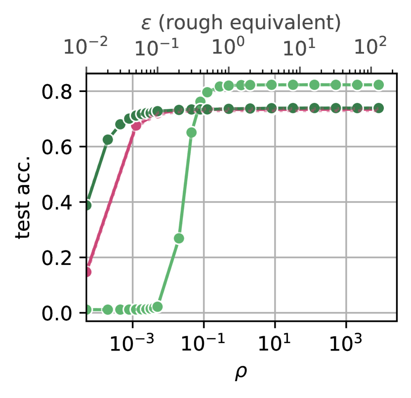
(a) IR=1.

(b) IR=10.

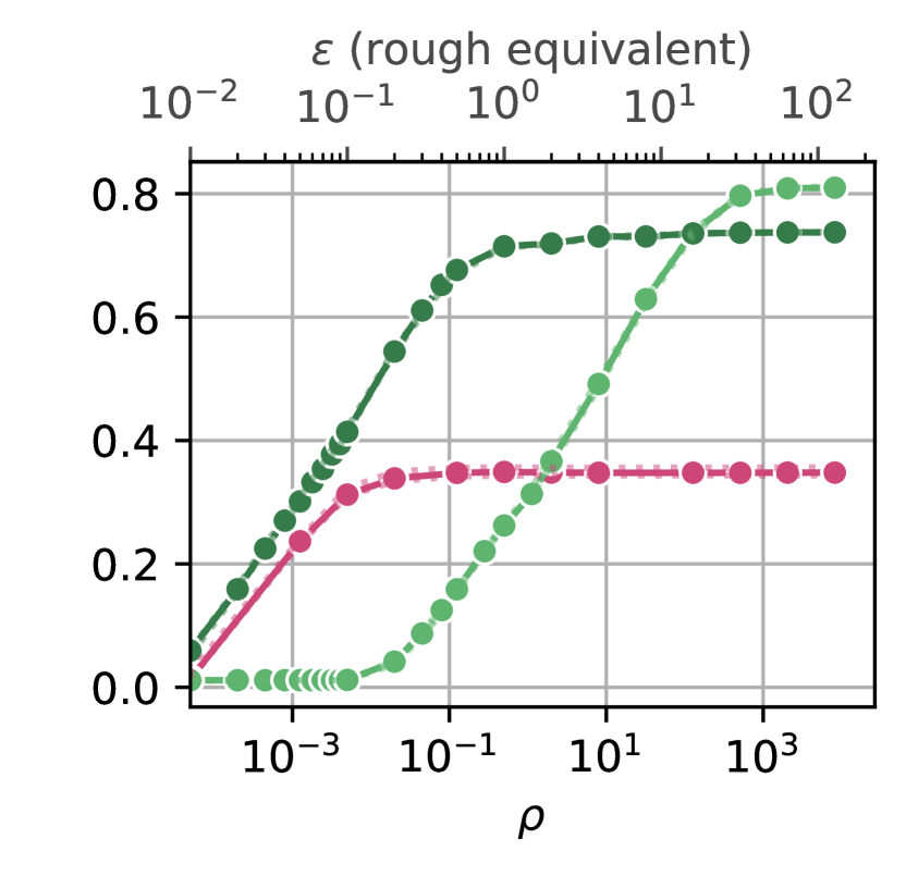
(c) IR=50.

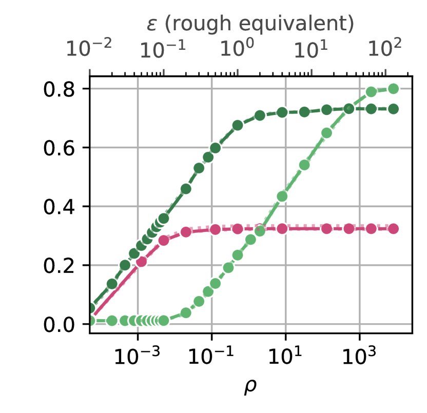
(d) IR=100.

Figure 2: DP Prototypes on CIFAR100. We present the balanced test accuracy of our methods vs. standard linear probing with DP-SGD on CIFAR100 and ViT-H-14 at different levels of imbalance rations (IR), using ImageNet as public data for DPPL-Public. We plot the mean test accuracy over multiple runs and represent the upper and lower quantiles for all methods by the dotted lines.

5.1 DP Prototypes Yield High Utility in High Privacy Regimes and under Extreme Imbalance

We evaluate our DP prototypes at different privacy regimes in the range corresponding to standard approximate DP [28] of $0.01<\varepsilon<100$ and under different IRs. In Figure 2, we benchmark our methods vs. standard DP linear probing on CIFAR100 with ViT-H-14. Our results highlight that over all levels of IRs larger than 1, our DPPL-Public significantly outperforms linear probing in all privacy regimes. Additionally DPPL-Public yields strong performance already at very low $\varepsilon$, such as $\varepsilon=0.1$ for IR=1. As data becomes more imbalanced, all methods require larger privacy budgets to yield similarly high performance. Further, our results indicate that our DPPL-Mean method underperforms DPPL-Public and DP linear probing for low $\varepsilon$. We find that this results from the noise added during the mean calculation leading diverging estimations. We provide further detail on the cause in Section C.2. Yet, we observe that at higher epsilon, DPPL-Mean outperforms DPPL-Public. This suggests that the most beneficial way for leveraging DP prototypes might be an adaptive method where DPPL-Public is chosen for high performance in the high privacy regimes and DPPL-Mean can further boost performance for larger $\varepsilon$.

We further assess whether the observed trend holds over different datasets. Therefore, we depict the results of our methods vs. standard DP linear probing for different datasets and the ViT-H-14 encoder under the most challenging setup with IR$=100$ in Figure 3. The observed trends are indeed consistent between all datasets. We provide full results over all datasets and IRs in Section E.1.

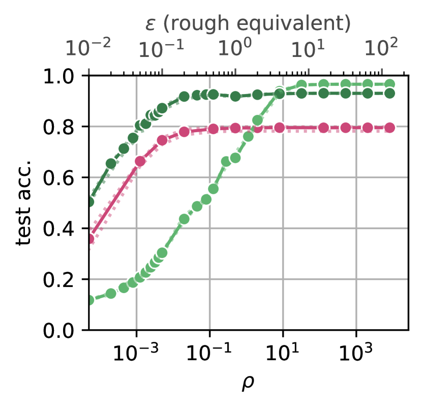
(a) CIFAR10

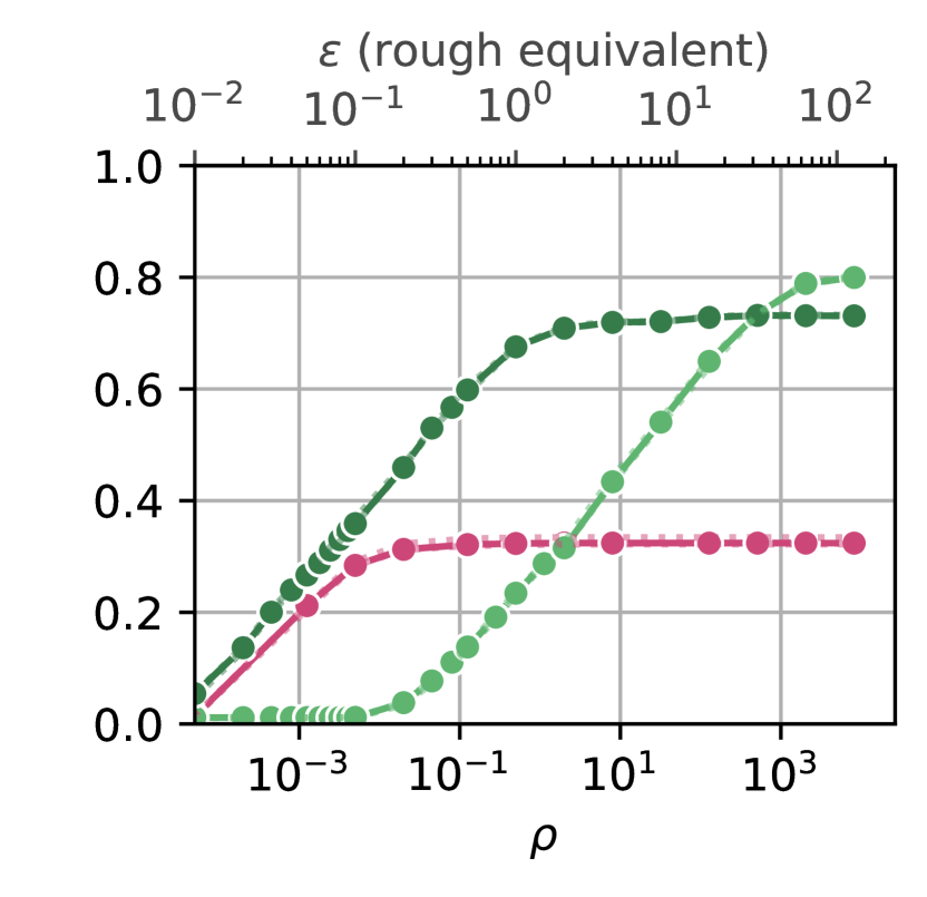
(b) CIFAR100.

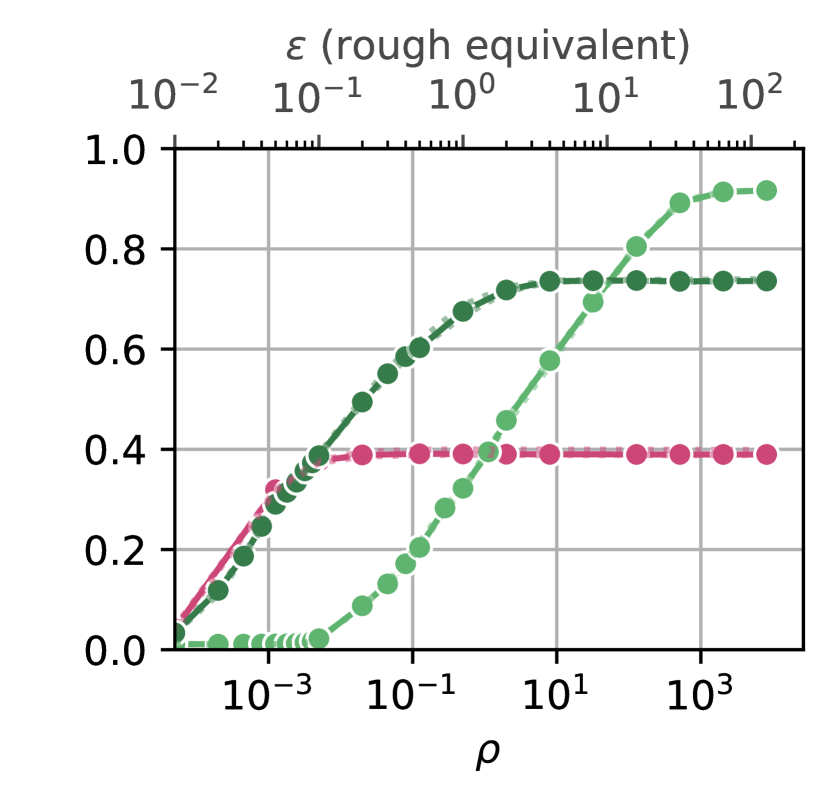
(c) FOOD101

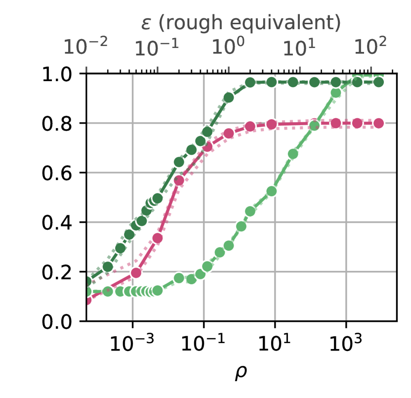
(d) STL10

Figure 3: DP Prototypes on various imbalanced datasets. We present the balanced test accuracy for CIFAR10, CIFAR100, FOOD101 and STL10 at an imbalance ratio of $100$ on ViT-H-14, using ImageNet as public data for DPPL-Public. We compare to standard Linear Probing with DP-SGD. We plot the mean test accuracy over multiple runs and represent the upper and lower quantiles for all methods by the dotted lines. See the full set of results in Section E.1.

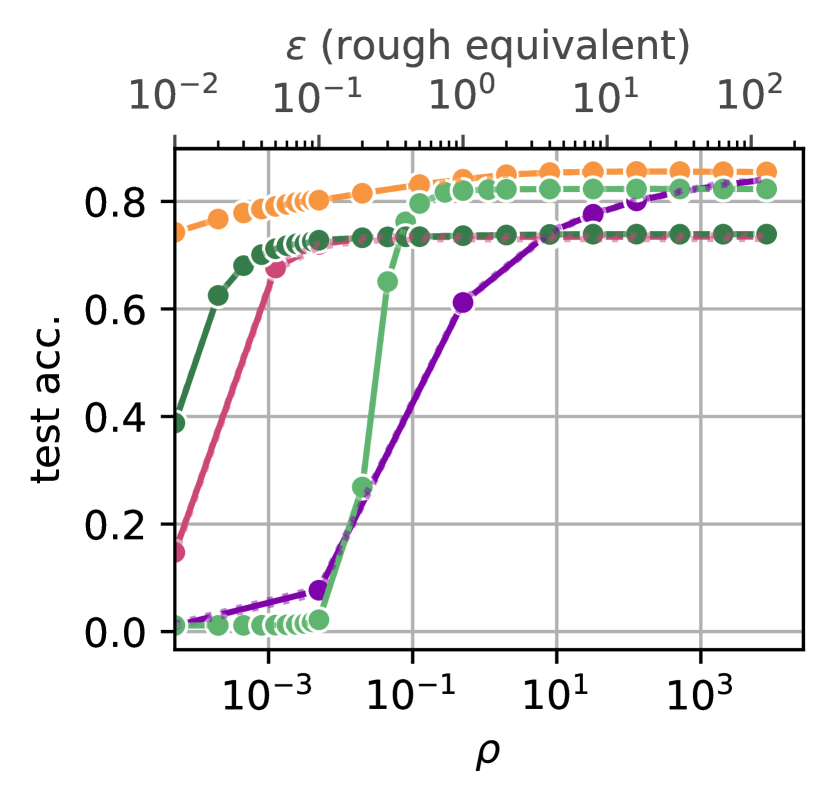
(a) IR=1.

(b) IR=10.

(c) IR=50.

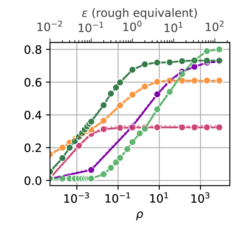
(d) IR=100.

Figure 4: Comparing against baselines on CIFAR100. We present the results of our methods vs. state-of-the-art methods (DP-LS by Mehta et al. [54] and DPSGD-Global-Adapt by Esipova et al. [29]) on the CIFAR100 dataset using ViT-H-14 under different IRs. DPPL-Public uses ImageNet as public data. Dotted lines represent the upper and lower quantiles for all methods. Similar results for CIFAR10, Food101, and STL10 can are presented in Appendix E.1.

5.2 DP Prototypes Improve over State-of-the-Art Baselines in Imbalanced Setups

We further benchmark our methods against DP-LS, the current state-of-the-art method for private transfer learning by Mehta et al. [54], and DPSGD-Global-Adapt by Esipova et al. [29], a DP method deliberately designed to achieve high utility under imbalancedness of the private data.

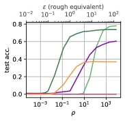
Figure 5: Minority Acc.

Our results in Figure 4 highlight that while in the balanced setup, Mehta et al. [54] outperforms the other methods, our DP prototypes outperform all other methods the more imbalanced the setup becomes. In particular DPPL-Public outperforms in high privacy regimes (i.e., for small $\varepsilon$), while DPPL-Mean is more suitable in lower privacy regimes where it matches or even outperforms DPSGD-Global-Adapt.

The advantage of our methods against the baselines become even more obvious as we do not consider the accuracy over the entire balanced test set (equivalent to balanced accuracy), but look specifically at accuracy on minority classes, see Figure 5. Therefore, we take the smallest $25\%$ of training classes in terms of number of their training data points and measure their accuracy on a balanced test set consisting of only those classes. Our results for CIFAR100 on ViT-H-14 under IR$=50$ in Figure 5 highlight that our DP prototypes significantly outperform all baselines. Full results for all datasets and minority classes are depicted in Section E.2.

5.3 Understanding the Success of DP Prototypes

To better understand the success of our DP prototypes, we perform various ablations. The full set of ablations and their results is presented in Appendix C.

(a) ViT-B-16.

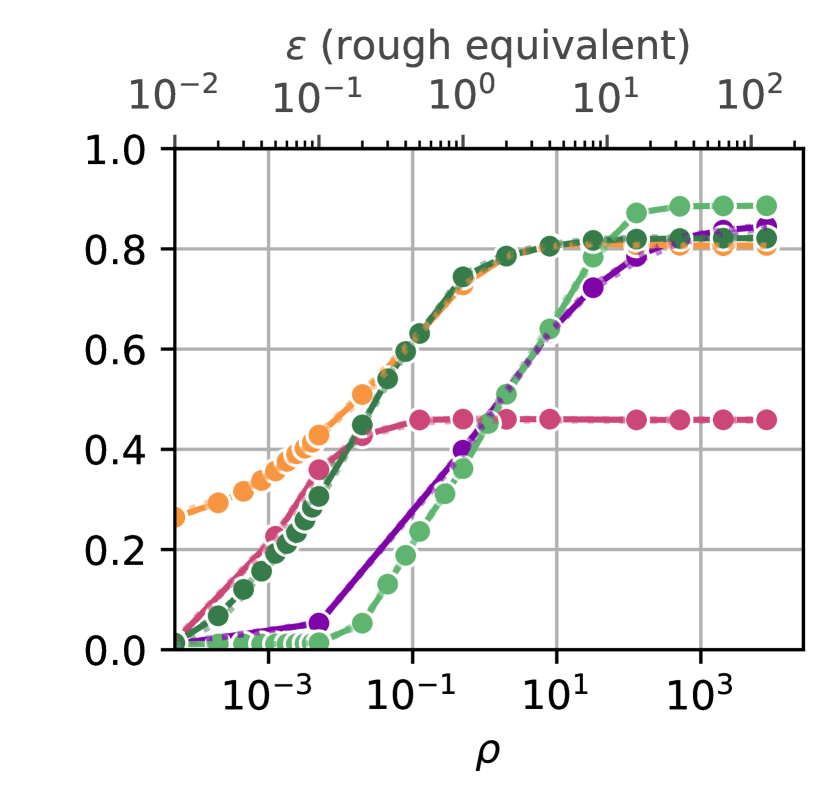
(b) ViT-L-16.

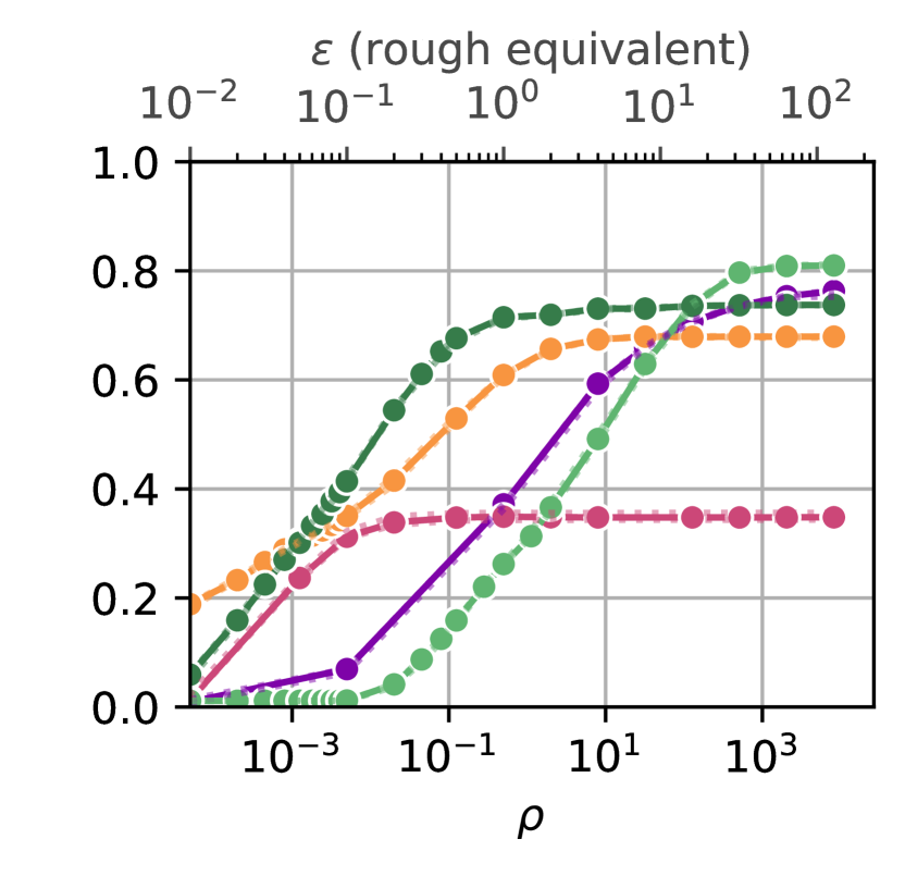
(c) ViT-H-14.

(d) ResNet-50.

Figure 6: Choice of Encoder. We report the test accuracy for our methods and the baselines for CIFAR100, using ImageNet as public data for DPPL-Public. We observe that the success of all methods depends on the quality of the underlying encoder.

Effect of the Publicly Pre-trained Encoder.

We first assess the impact of the encoder used as a feature extractor. Therefore, we apply our method and the baselines with different encoder architectures. Our results in Figure 6 highlight that the encoder performance impacts all methods alike. In particular, we observe that all methods obtain better results with stronger encoders. For example, the ViT-H-14 yields to significantly higher private prediction accuracy that the much smaller ViT-B-16. Additionally, none of the methods yields satisfactory results using the ResNet50.

Impact of the Projection Layer.

We evaluate whether a projection layer, usually part of a prototypical network, can increase the utility. We present our results in Figure 8 for CIFAR100 on ViT-H-14, using ImageNet as public for DPPL-Public. They highlight that DPPL-Public does not benefit from the projection. Even non-privately ($\epsilon=\infty$), the accuracy of DPPL-Public with projection is $72.6\%$ and without projection is $74.0\%$, showing that it is not just the decreased privacy budget for the sampling that reduces the utility, but a fundamental misalignment between how the projection is trained and the public prototyping. We observe the same effect for DPPL-Mean and conclude that with a strong enough pre-trained encoder, it is sufficient for DPPL to estimate prototypes without projection.

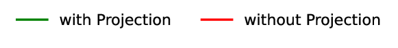
(a) DPPL-Public.

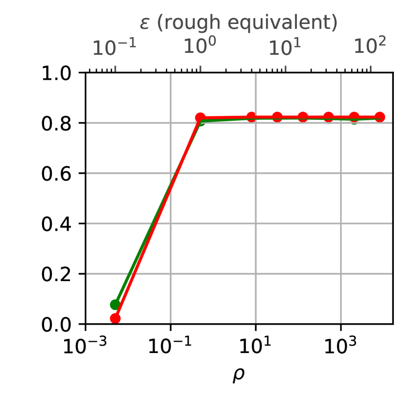
(b) DPPL-Mean.

Figure 7: Impact of the Projection Layer.

(c) Public Distribution.

(d) Public Data Size.

Figure 8: Impact of the Public Data.

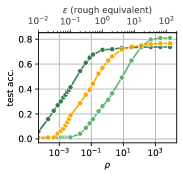
Figure 9: Top-K.

Improving through Multiple Per-Class Prototypes.

We experiment with extending our DPPL-Public beyond a single per-class prototype—the common standard for prototypical networks. Therefore, we introduce the variation DPPL-PublicK which selects the top-K public prototypes per class. For the private top-K selection, we extend the algorithm from Gillenwater et al. [33] to sample these multiple prototypes jointly using the exponential mechanism. Then, we classify based on the mean distance to each class’s prototype. Our results in Figure 9 show that DPPL-PublicK’s privacy-utility trade-offs are between DPPL-Mean and DPPL-Public. This shows that the private means can be approximated by multiple public prototypes. DPPL-PublicK could therefore replace DPPL-Mean in cases of high dimensionality, where a mean estimation is not feasible. We provide a detailed description of the method, privacy proof, and a full set of results in Section C.3.

Impact of the Public Data for Prototype Selection.

To assess whether the public data for prototype estimation needs to be from the same distribution as the one used to pre-train the encoder, we conduct experiments with a different public dataset. We evaluate DPPL-Public using 2,298,112 samples from CC3M introduced by Sharma et al. [65] as public data instead of ImageNet which is used to pre-train the encoder. We show the relation between the accuracy using ImageNet as public data and CC3M in Figure 7(c) for CIFAR100 on ViT-H-14. We find that DPPL-Public works well with both public datasets, highlighting the flexibility of our approach. Still, we observe that ImageNet yields slightly better results which suggests that it is particularly beneficial to levergae the public data already available for pre-training also in the private transfer learning step.

Size of the Public Dataset for DPPL-Public.

We also evaluate the success of DPPL-Public for different sizes of the public dataset that the public prototypes can be chosen from. Therefore, we randomly draw subsets of different sizes from ImageNet and apply DPPL-Public. Our results for CIFAR100 (100 classes) and ViT-H-14 in Figure 7(d) indicate that with growing public dataset size, our method’s success increases. Note that even for public dataset of more than one million images, the selection of our public prototypes for 100 classes (i.e., the "training") takes only 34.3 seconds on a single GPU as we depict in Table 2. For 10 classes (e.g., CIFAR10), it takes only 5 seconds. Hence, choosing a larger public dataset does not represent a practical limitation.

6 Conclusions and Future Work

We propose DPPL as a novel alternative to private fine-tuning with DP. DPPL builds DP prototypes on top of features extracted by a publicly pre-trained encoder, that can be later used as a classifier. The prototypes can be obtained without iterative noise addition and yield high utility even in high-privacy regimes, with few private training data points, and in unbalanced training setups. We show that we can further boost performance of our DP prototypes by leveraging the public data beyond training of the encoder and using them to draw the public prototypes from (DPPL-Public). Future work at improving utility of high-dimensional DP mean estimation will benefit our DPPL-Mean, which can, in the future, serve as an additional benchmark for private mean estimation algorithms.

Appendix A Extended Background

A.1 Differential Privacy

Definition 1 ($(\xi,\rho)$-zCDP from Bun and Steinke [13])

A randomised mechanism $M:\mathcal{X}^{n}\rightarrow\mathcal{Y}$ is $(\xi,\rho)$-zero-concentrated differentially private (henceforth $(\xi,\rho)$-zCDP) if, for all $x,x^{\prime}\in\mathcal{X}^{n}$ differing on a single entry and all $\alpha\in(1,\infty)$,

$$\mathrm{D}_{\alpha}\left(M(x)\|M\left(x^{\prime}\right)\right)\leq\xi+\rho\alpha,$$

where $\mathrm{D}_{\alpha}\left(M(x)\|M\left(x^{\prime}\right)\right)$ is the $\alpha$-Rényi divergence between the distribution of $M(x)$ and the distribution of $M\left(x^{\prime}\right)$.

$(0,\rho)$-zCDP can also be expressed simply as $\rho$-zCDP.

Definition 2 ($(\alpha,\epsilon)$-RDP from Mironov [55])

A randomized mechanism $f:\mathcal{D}\mapsto$ $\mathcal{R}$ is said to have $\epsilon$-Rényi differential privacy of order $\alpha$, or $(\alpha,\epsilon)$-RDP for short, if for any adjacent $D,D^{\prime}\in\mathcal{D}$ it holds that

$$D_{\alpha}\left(f(D)\|f\left(D^{\prime}\right)\right)\leq\epsilon.$$

Definition 3 ($\mu$-GDP from Dong et al. [24])

A randomized mechanism $M:\mathcal{D}\mapsto$ $\mathcal{R}$ is said to have $\mu$-Gaussian differential privacy, $\mu$-GDP for short, if it operates on a statistic $\Theta$ as

$$M(D)=\Theta(D)+\xi$$

where $\xi\sim\mathcal{N}(0,\text{sens}(\theta)^{2}/\mu^{2})$

A.2 The Gaussian Mechanism

Proposition 1 (Cesar and Rogers [17])

Let $q:\mathcal{X}^{n}\rightarrow\mathbb{R}$ be a sensitivity-$\Delta$ query. Consider the mechanism $M:\mathcal{X}^{n}\rightarrow\mathbb{R}$ that on input $\mathbf{x}$, releases a sample from $\mathcal{N}\left(q(\mathbf{x}),\sigma^{2}\right)$. Then $M$ satisfies $\left(\Delta^{2}/2\sigma^{2}\right)$-zCDP.

A.3 The Exponential Mechanism

The exponential mechanism [51] aims to give the best output $\hat{\mathbf{x}}\in\hat{\mathbf{X}}$ w.r.t. a utility function $u(\mathbf{X},\hat{\mathbf{x}}):\mathbf{X}\times\hat{\mathbf{X}}\rightarrow\mathbb{R}$ where $\mathbf{X}$ is a private dataset and $\hat{\mathbf{X}}$ a public dataset. It can be described as a randomized mapping $\text{EM}_{u}:\mathbf{X}\rightarrow\hat{\mathbf{X}}$ where

$$P[\text{EM}_{u}(\mathbf{X})=\hat{\mathbf{x}}]\propto\exp{\left(\frac{\epsilon}{\Delta u}u(\mathbf{X},\hat{\mathbf{x}})\right)}$$ (4)

Lemma 1 (McSherry and Talwar [51])

The exponential mechanism is $2\epsilon$-DP.

Definition 4

A utility function $U(D,\mathbf{x})$ is positively (negatively) monotonic if for any point $\mathbf{x}$ and any datasets $D$ and $D^{\prime}$, $U(D,\mathbf{x})\leq U(D\cup D^{\prime},\mathbf{x})$$\quad\left(U(D,\mathbf{x})\geq U(D\cup D^{\prime},\mathbf{x})\right)$.

Lemma 2 (McSherry and Talwar [51])

Given a monotonic utility function, the exponential mechanism is $\epsilon$-DP.

The exponential mechanism fulfils not only differential privacy, but also the stricter bounded range [27]. Using a monotonic utility function leads to an improved privacy bound because the sensitivity and range of monotonic functions are equal [25].

Lemma 3 (Cesar and Rogers [17])

The $\epsilon$-DP exponential mechanism is $\epsilon^{2}/8$-zCDP.

A.4 Mean Estimation

The CoinPress algorithm [25] aims to privately estimate the mean $\mathbf{\mu}=1/n\sum_{n}\mathbf{x}$ for some private $\mathbf{x}\in\mathbb{R}^{d}$. Each step is initiated with a center $\mathbf{c}_{i}$ and radius $r_{i}$ with $||\mu-c_{i}||_{2}\leq r_{i}$. Commonly used for $(r_{0},c_{0})$ are $(\sqrt{d},\mathbf{0})$. All points further away from $\mathbf{c}_{i}$ than $r_{i}+\gamma$, where $\gamma$ is chosen s.t. $\Pr[||\mathcal{N}(\mathbf{0},d)||_{2}<\gamma]\geq 0.99$ are $\ell_{2}$-clipped to $r_{i}+\gamma$. Finally, Gaussian noise is added to all points. Then $\mathbf{c}_{i+1}$ is the mean of the noised and clipped points and $r_{i+1}$ defined through the new Gaussian tailbounds of the points.

Appendix B Extended Experimental Setup

B.1 Computational Resources and Libraries

Our implementation is in Jax [9]. Private linear probing was conducted with PyTorch [61] and made private using the Opacus [78] privacy engine. We relied on Optuna [2] using the Tree-structured Parzen Estimator [5] for all algorithmic hyperparameter optimizations. Converting and visualizing privacy guarantees was done in part with AutoDP [75, 81]. Scaling the experiments has been aided by Ray [56] and Dask [64]. Configurations were handled by Hydra [77]. The experiments were conducted using NVIDIA A100 GPUs. In total, obtaining all results required approximately $300$ GPU hours, resulting in roughly $105$ kWh of electric energy usage.

B.2 Imbalanced Datasets

We present the distribution of the number of data points per class in Table 1 and Figure 10

Table 1: Number of data points over different rations of imbalance. Median and average number of samples per class for each dataset and imbalance ratio. We construct the imbalanced datasets as described in Cui et al. [20] and subsequently Cao et al. [14] (Exponential Long-Tailed).

Dataset	Imbalance Ratio
	1		10		50		100
	Median	Mean	Median	Mean	Median	Mean	Median	Mean
CIFAR10	5000		1594	2043	724	1340	517	1241
CIFAR100	500		158	196	71	127	50	109
FOOD101	750		237	297	106	190	75	163
STL10	500		160	204	73	140	52	124

(a) All IRs.

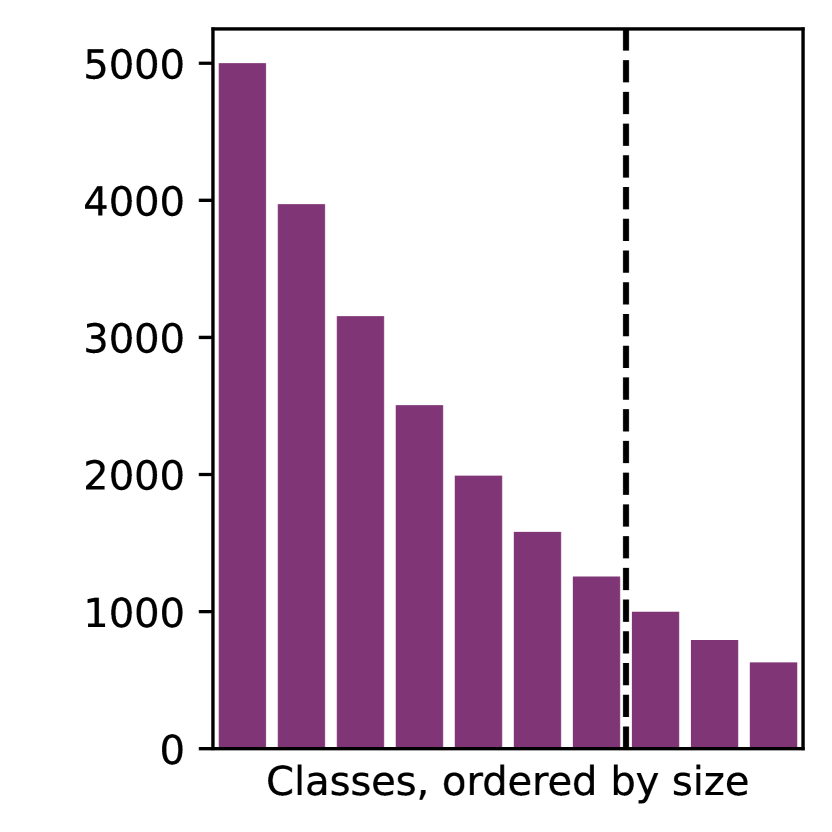
(b) IR=10.

(c) IR=100.

Figure 10: Visualizing the effect of the imbalance on CIFAR10. We order the classes by the number of corresponding samples and plot them. The classes right of the dotted line are considered to be the minority classes.

Appendix C Ablations

C.1 Public Dataset Size

The public data used for DPPL-Public, ImageNet, consists of 1,281,167 samples. We evalute the impact of using a smaller public dataset by randomly subsampling. Figure 11 shows the resulting accuracy. The accuracy and amount of public samples are positively correlated in all cases, but for some datasets, i.e., CIFAR10, STL10, the accuracy seemingly asymptotically approaches a maximum accuracy. For FOOD101 it seems ImageNet is not large enough. We note that the imbalance ratio doesn’t change the amount of public data required.

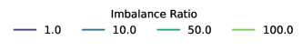
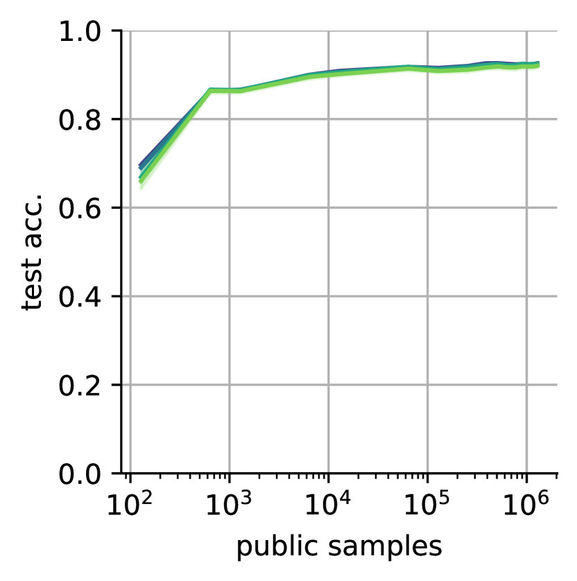
(a) CIFAR10.

(b) CIFAR100.

(c) STL10.

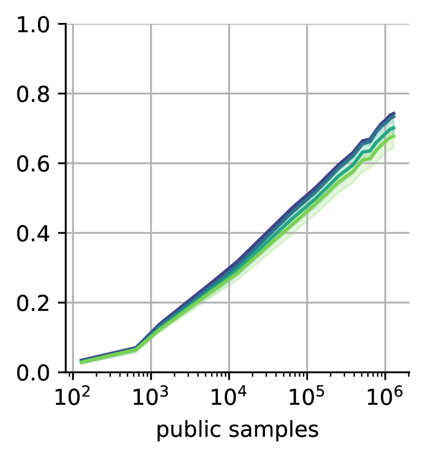
(d) FOOD101.

Figure 11: Varying public dataset sizes for DPPL-Public. We randomly subsample the public dataset, limiting DPPL-Public’s prototype selection to fewer samples, and evaluate the resulting changes in accuracy.

C.2 Mean Estimation

Figure 12 shows how the private means estimation behaves for reasonable and too low privacy levels. For too low privacy values, the mean estimation breaks down. We identify the underlying cause as the divergence of the bounding radius and visualize it in Figure 13. Each successive radius is supposed to be decreasing in size, successively bounding the estimated mean to a smaller space. This is achieved by taking the mean of clipped and noised samples. The clipping decreases the average norm and thus reduces the radius. For very low privacy budgets, the noising of the samples outweighs this effect, and the norms instead grow with each step, leading to a diverging radius. As we take the mean of increasingly diverging samples, the estimates of the mean diverge.

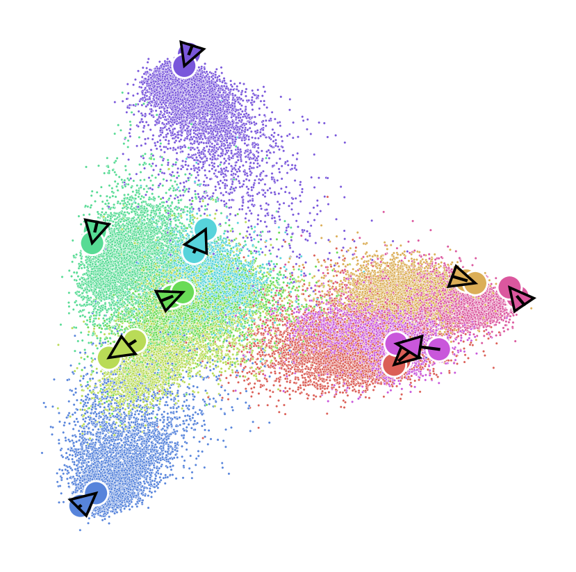
(a) $\rho=10^{-3}$: True vs. DP means.

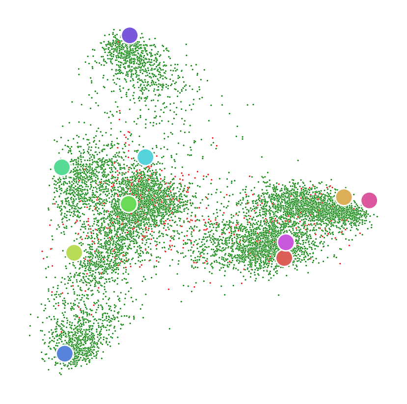
(b) $\rho=10^{-3}$: Classification results.

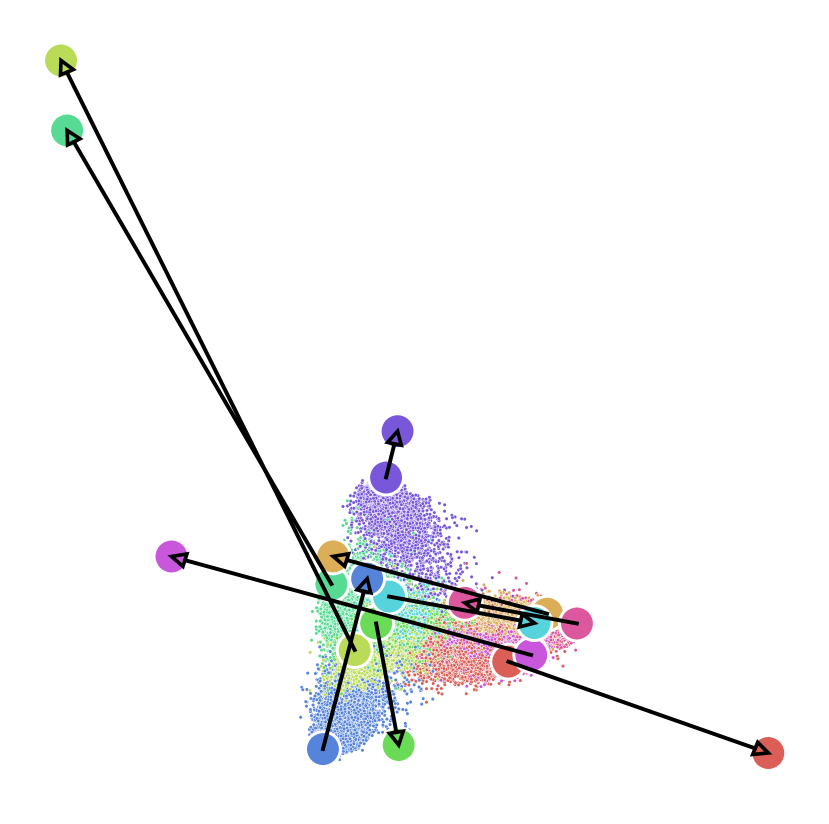
(c) $\rho=10^{-4}$: True vs. DP means.

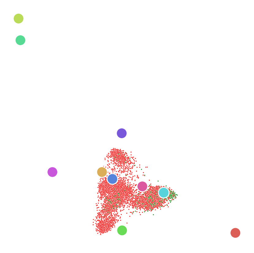
(d) $\rho=10^{-4}$: Classification results.

Figure 12: Visualizing the mean estimation on CIFAR10. We estimate the means using CoinPress [7] at $\rho\in\{10^{-3},10^{-4}\}$. On the left, we show the non-private means and connect them with arrows to the privately estimated ones on top of the train set. Colors indicate the classes. On the right, we show the privately estimated means and the test set. Green points represent correctly classified samples, red points misclassified ones.

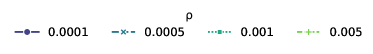
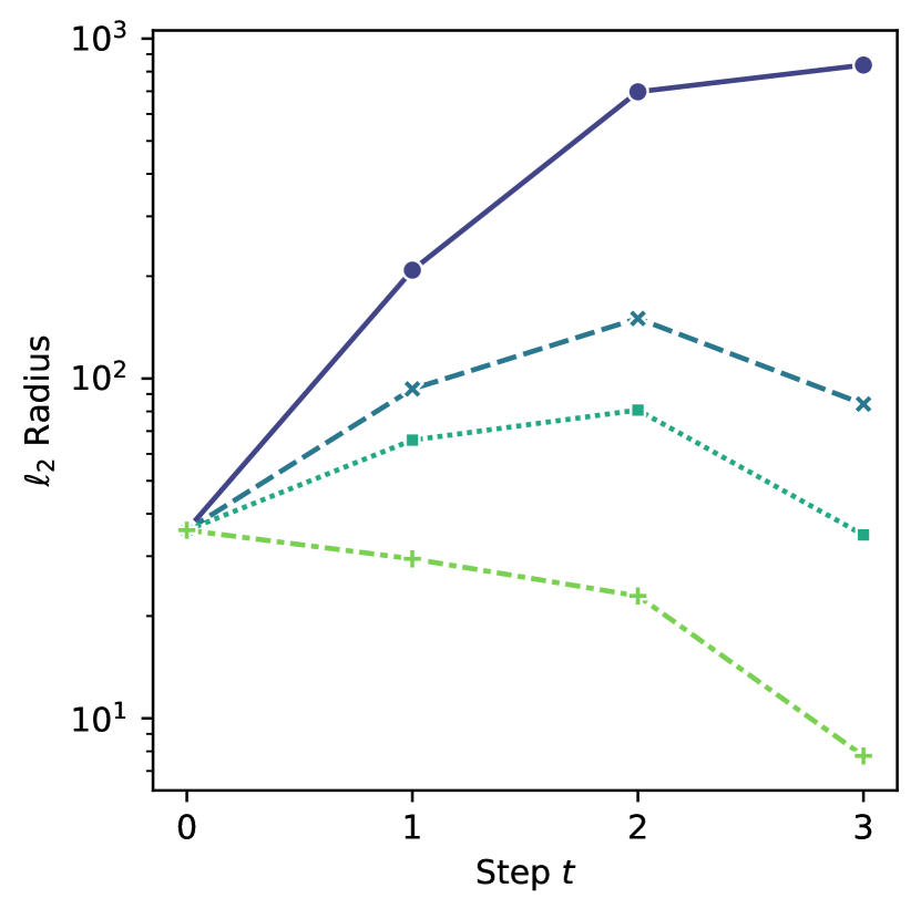
(a) Radius.

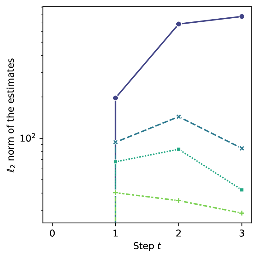
(b) Norm of the estimation.

Figure 13: Analyzing the steps of CoinPress. We estimate the means using CoinPress [7] for different $\rho$. We see that for low values of $\rho$, the radius and the estimates diverge.

C.3 Top-K Public Prototyping

Prototypical Networks have been extended to two prototypes per class, leading to increased generalization and robustness [69]. We generalize this concept to $K$ prototypes per class. We propose our Differentially Private Unordered Top-$K$ Selection as an adaption of the algorithm from Gillenwater et al. [33] to sample these multiple prototypes jointly using the exponential mechanism.

C.3.1 Differentially Private Unordered Top-$K$ Selection

Let $(u_{1},\dots,u_{n})$ be the utilities of the public samples in decreasing order and $K$ the number of prototypes to select. Since the order of the prototypes is not important in this context, we define the utility $U(\mathbf{X},S)$ of a set of prototypes $S=\{u_{S_{1}},\cdots,u_{S_{K}}\}$ w.r.t. the private datasets $\mathbf{X}$ as

$$U(\mathbf{X},S)=\begin{cases}-u_{K}+\min_{k\in[K]}u_{s_{k}}&\text{ if }s_{1},\ldots,s_{K}\\ &\text{ are distinct. }\\ -\infty&\text{ otherwise }\end{cases}$$ (5)

Lemma 4

$\Delta U=\Delta u$.

Proof. The choice of $-\infty$ for repeating sequences does not depend on the private data and therefore doesn’t affect the sensitivity. Furthermore, the utility of a set is only dependent on the lowest utility in the set $u_{\min{}}$ and the $K$th true best utility $u_{K}$. The utility of a set can thus be formulated as $U(\mathbf{X},S)=u_{K}-u_{\min}$. $u$ is monotonic and has sensitivity $\Delta u$, in other words, insertion of a private sample can only increase each utility $u$ by a maximum of $\Delta u$. It follows that insertion or removal of a private sample can only change $U$ by $\pm\Delta u$, i.e., $\Delta U=\Delta u$

Therefore, each set has the utility of its worst entry, unless two entries repeat, in which case the utility is $-\infty$ and such set therefore never selected. If we select the true $K$-best prototypes, the utility is $0$ and otherwise it’s negative. Each utility is not unique. Instead, a utility can occur as many times as the number of possible combinations of samples with a higher utility. Given a utility $u_{y}$, we can therefore obtain the number of possible sets with that utility

$$m(u_{y})={y\choose K}$$ (6)

The entire algorithm then consists of

1. privately sampling a utility $u_{y}$ with $P[EM(x)=y]\propto{y\choose K}\exp{\frac{\epsilon u_{y}}{2\Delta U}}$,

2. fixing the corresponding $\hat{\mathbf{x}}_{y}$ as part of the set, and

3. uniformly sampling the remaining $K-1$ prototypes without replacement, s.t. $\{\hat{\mathbf{x}}_{i}|u_{i}\geq u_{y}\}$.

Note that while Lemma 4 implies the sensitivity of $u$ and $U$ are the same, our effective privacy costs still double, since $U$ is no longer monotonic. We perform the sampling using Proposition 5 from Medina and Gillenwater [52].

C.4 Classification with Multiple Prototypes

Given $K$ multiple prototypes $\mathbf{P}_{c}\in\mathcal{R}^{K\times d}$ for each class $c\in[C]$, we classify $\mathbf{x}$ based on the minimum average distance

$$f(\mathbf{x})=\underset{c}{\arg\min}\frac{1}{K}\sum_{i=1}^{K}d(\mathbf{x},\mathbf{p}_{c,k})\text{.}$$ (7)

ViT-B-16

ViT-L-16

ViT-H-14

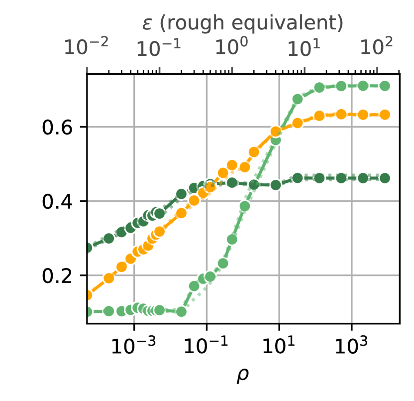
(b) IR=10.

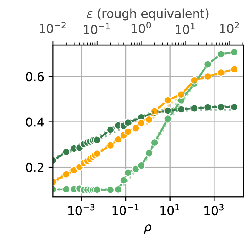
(c) IR=50.

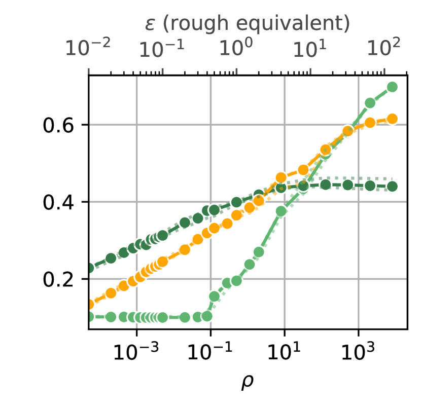
(d) IR=100.

Figure 14: DPPL-Public  with Top-$K$. We present the results including DPPL-Public Top-$K$ of CIFAR10 on ViT-B-16, ViT-H-14, ViT-L-16 and ResNet-50, using ImageNet as public data for DPPL-Public, at different levels of imbalance rations (IR).

ResNet-50

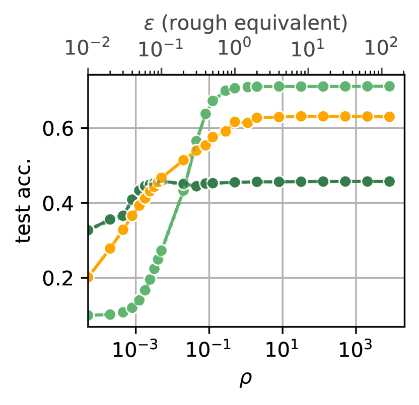
(a) IR=1.

ViT-B-16

ViT-L-16

ViT-H-14

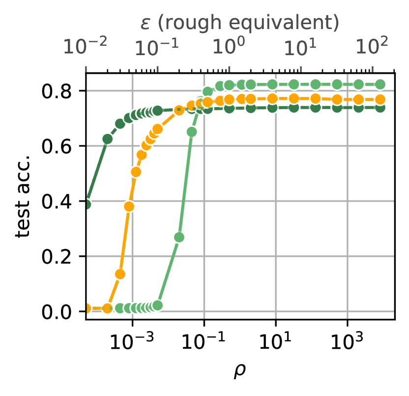
(b) IR=10.

(c) IR=50.

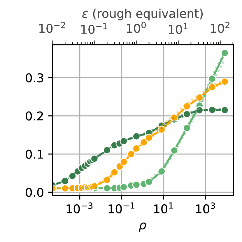
(d) IR=100.

Figure 15: DPPL-Public  with Top-$K$. We present the results including DPPL-Public Top-$K$ of CIFAR100 on ViT-B-16, ViT-H-14, ViT-L-16 and ResNet-50, using ImageNet as public data for DPPL-Public, at different levels of imbalance rations (IR).

ResNet-50

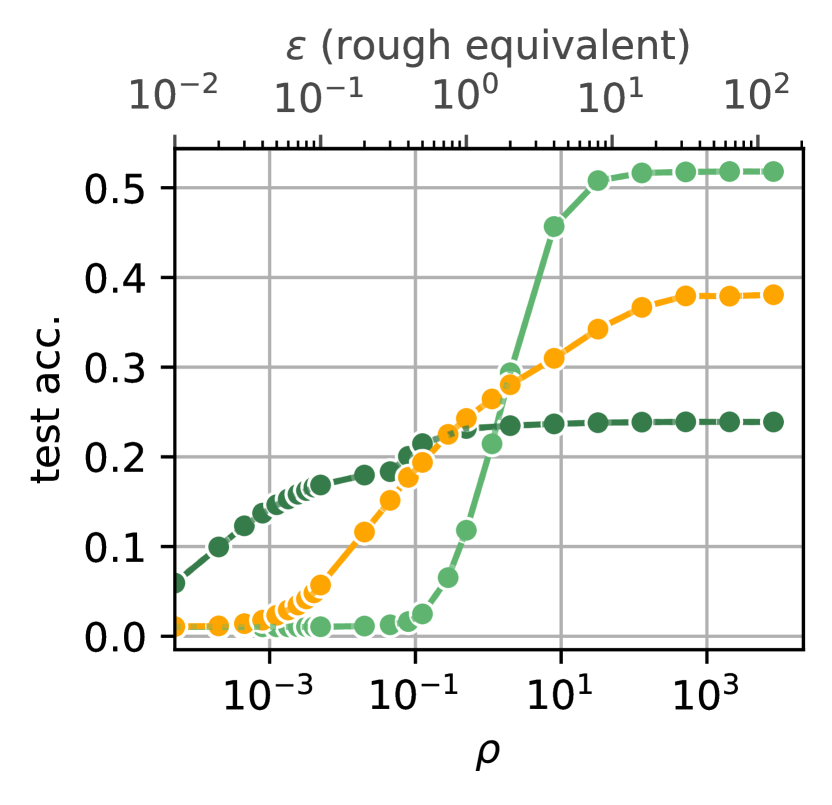
(a) IR=1.

ViT-B-16

ViT-L-16

ViT-H-14

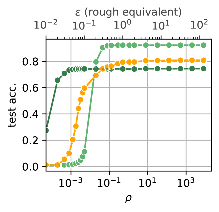
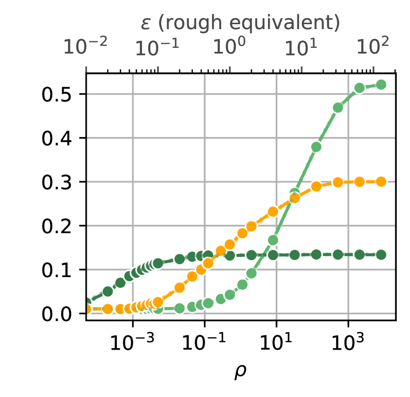
(b) IR=10.

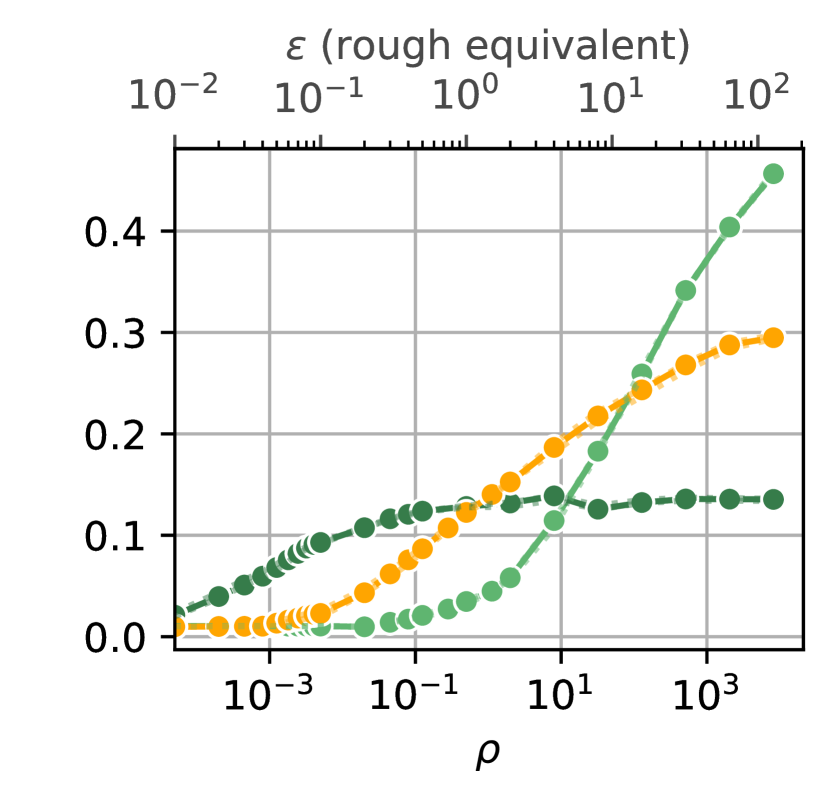
(c) IR=50.

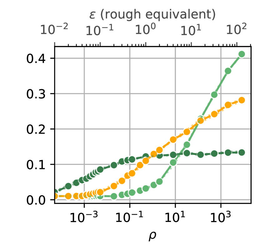
(d) IR=100.

Figure 16: DPPL-Public  with Top-$K$. We present the results including DPPL-Public Top-$K$ of FOOD101 on ViT-B-16, ViT-H-14, ViT-L-16 and ResNet-50, using ImageNet as public data for DPPL-Public, at different levels of imbalance rations (IR).

ResNet-50

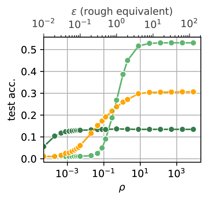
(a) IR=1.

ViT-B-16

ViT-L-16

ViT-H-14

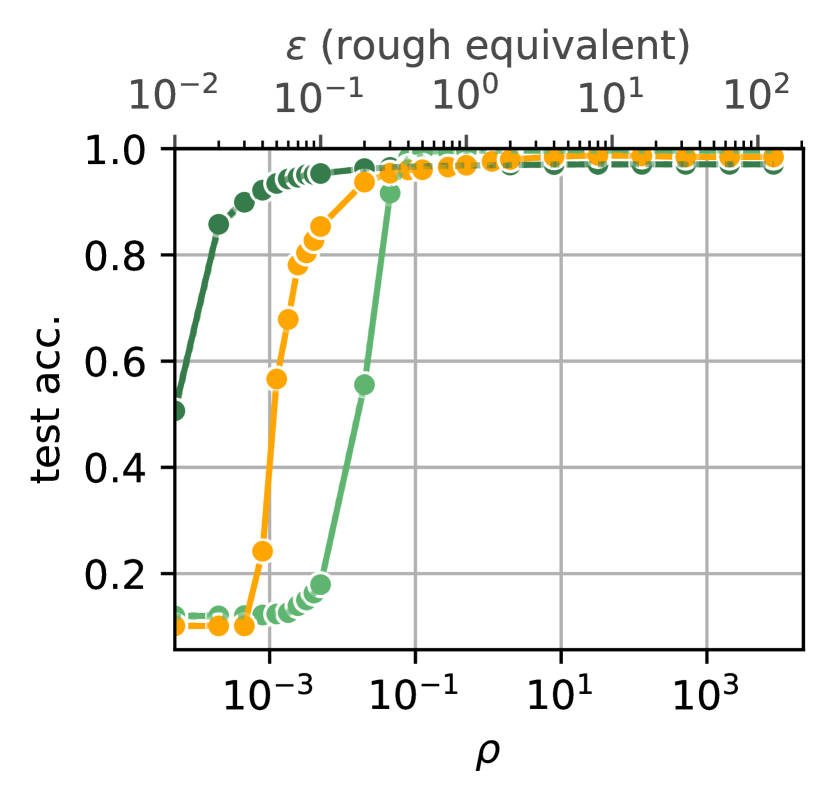
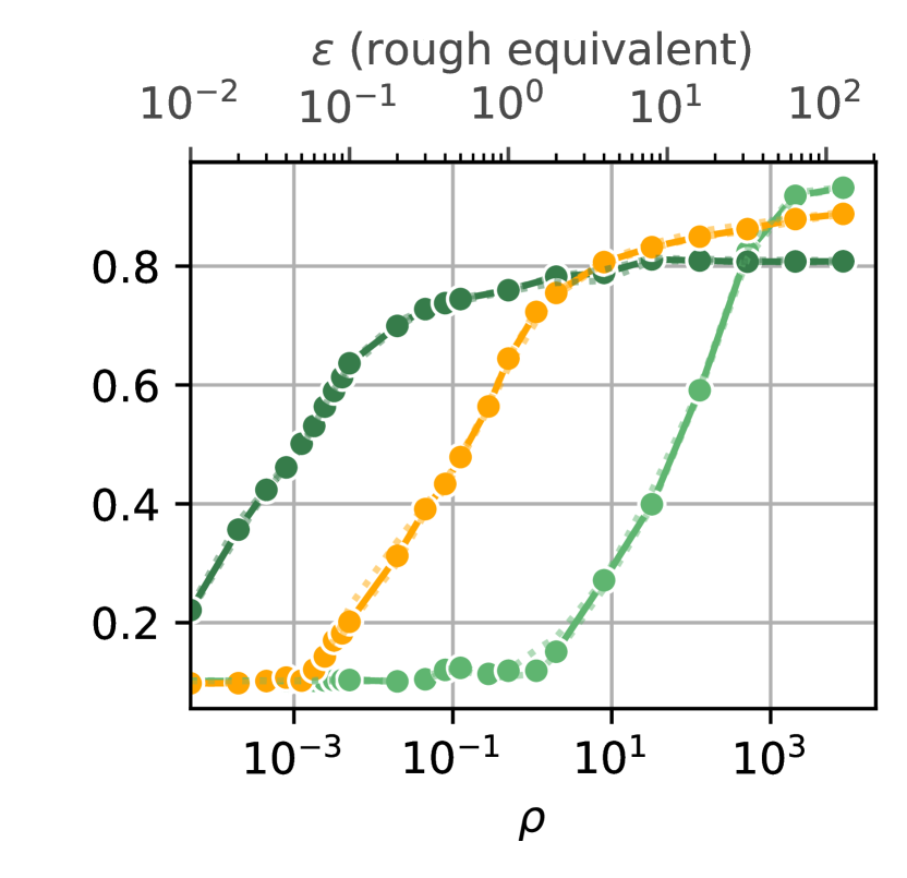
(b) IR=10.

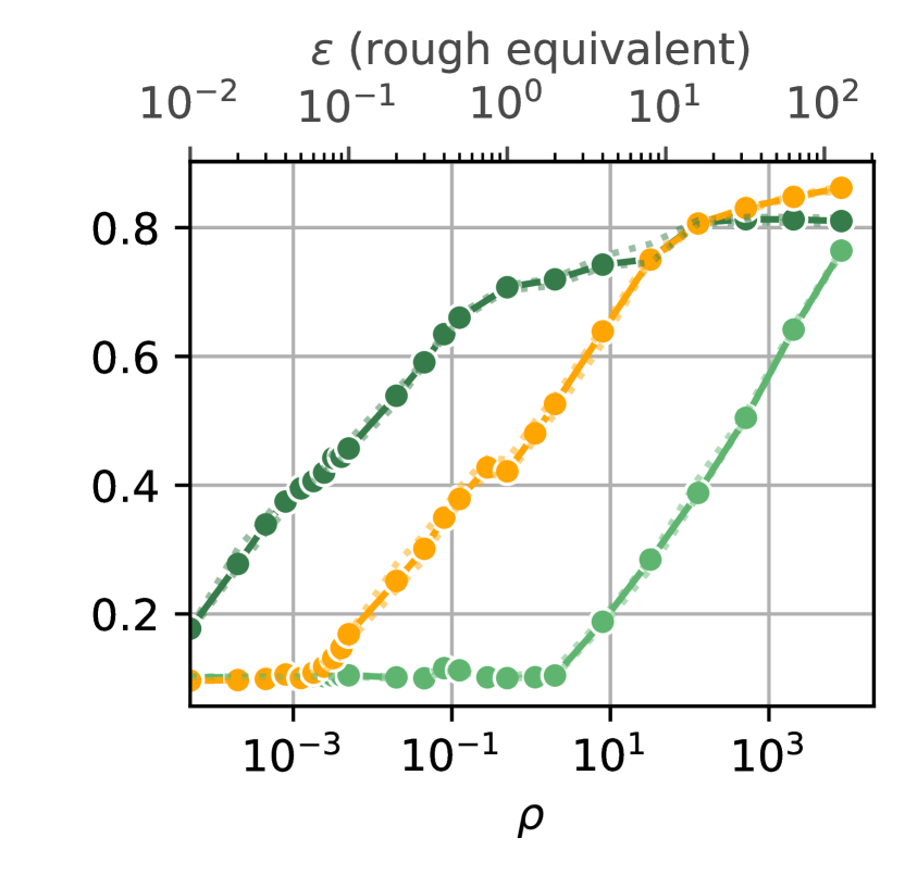
(c) IR=50.

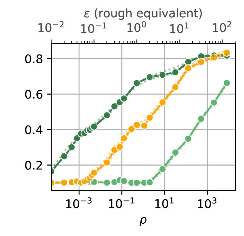
(d) IR=100.

Figure 17: DPPL-Public  with Top-$K$. We present the results including DPPL-Public Top-$K$ of STL10 on ViT-B-16, ViT-H-14, ViT-L-16 and ResNet-50, using ImageNet as public data for DPPL-Public, at different levels of imbalance rations (IR).

ResNet-50

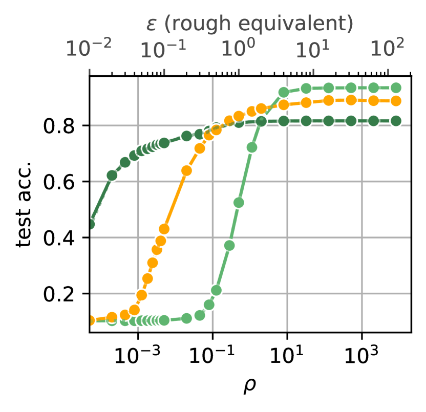
(a) IR=1.

C.4.1 Results

We sweep over $K\in[1,2,3,5,10,20]$ and sort by balanced train accuracy to find the optimal $K$ per privacy value, which Figure 18 shows. As we increase the privacy budget, the optimal accuracy is achieved at increasing $K$’s. For $\rho>100$ all $K_{\text{optimal}}$ converge to $K=10$. In this privacy regime, the Top-$K$ selection behaves essentially as it would non-privately. In this case, it seems to be detrimental to pick too many prototypes, although we note the accuracy of $K\in\{5,10,20\}$ is almost on par, being $76.7\%$, $77.1\%$ and $77.2\%$ respectively for $\rho=128$. Figure 9 shows the method requires a privacy budget somewhere between DPPL-Mean and DPPL-Public, while having a maximum accuracy also in between the maximum accuracy of those methods, closer to the higher accuracy of DPPL-Mean. We show the full set of results in Figures 14, 15, 16 and 17.

Figure 18: Optimal $K$ for Top-$K$

C.5 Projection

C.5.1 Setup

The projection consists of a single layer linear network $f:\mathbb{R}^{d_{\text{avg}}}\rightarrow\mathbb{R}^{d_{p}}$ with no activation function and an average pooling layer with kernel size $p_{\text{before}}\in[1,64]$ before the linear layer. As we leave the total privacy budget $\rho$ unchanged, we introduce a hyperparameter $s\in[0.1,0.9]$ which defines the privacy budget of the projection layer $\rho_{l}=s*\rho$ and of the prototype estimation $\rho_{p}=(1-s)*\rho$. In total, the hyperparameters are $s\in[0.1,0.9]$, $p_{\text{before}}\in[1,64]$, output dimension $d_{p}$, the number of augments per step $n$, batch-size, learning-rate, gradient clipping norm and number of training steps.

We train the projection with the original training rule from Snell et al. [68], with some adaptions for privacy. We perform Bernoulli sampling (often more generally referred to as Poisson sampling) to receive a batch $B=(\mathbf{X},\mathbf{y})$. We split $(\mathbf{X},\mathbf{y})$ evenly into support and query $(\mathbf{X}_{S},\mathbf{y}_{S}),(\mathbf{X}_{Q},\mathbf{y}_{Q})$, s.t. each part has the same number of samples per class. If a class has only one corresponding sample in $\mathbf{X}$, we drop it. The prototypes for each class $\mathbf{p}_{c}$ are estimated as the mean of samples in the support set $\mathbf{X}_{S}$ that have the corresponding class label in $\mathbf{y}_{S}$.

$$\mathbf{X}_{S,c}=\{\mathbf{x}_{i}\in\mathbf{X}_{S}|y_{i}=c\}$$ (8)

$$\mathbf{p}_{c}=\frac{1}{|\mathbf{X}_{S,c}|}\sum_{\mathbf{x}\in\mathbf{X}_{S,c}}\mathbf{x}$$ (9)

Then, prototypes and query samples are projected with the linear layer.

$$\mathbf{X}^{\prime}_{Q}=\{f(\mathbf{x})\ |\;\mathbf{x}\in\mathbf{X}_{Q}\}$$ (10)

$$\mathbf{p}^{\prime}_{c}=f(\mathbf{p}_{c})$$ (11)

Finally, the model aims to classify each sample in $\mathbf{X}^{\prime}_{Q}$ by assigning it the label of the closest prototype

$$\hat{\mathbf{y}}=\{\underset{c}{\arg\min}\;d(\mathbf{p}^{\prime}_{c},\mathbf{x}^{\prime})|\mathbf{x}^{\prime}\in\mathbf{X}^{\prime}_{Q}\}$$ (12)

We implement the classification training using a log-softmax over the distances to the prototypes and the negative log likelihood loss. This entire process, beginning with the split of $B$, is repeated $n$ times, before aggregating the loss and conducting the private gradient descent on the projection layer weights.

C.5.2 DPPL-Mean

For DPPL-Mean we expected the reduction in dimensionality to potentially improve to utlity-privacy-tradeoff, but instead higher dimensions were strictly better, leading to the removal of $p_{\text{before}}$ and $d_{p}$ as hyperparameters. We show in Figure 19 the distribution of accuracyies during the hyperparameter optimization and that no configuration reached the performance without projection.

C.5.3 DPPL-Public

For DPPL-Public, we additionally need to project the public data embeddings, to find the prototypes in the projected latent space. Furthermore, we found that the utility is strictly lower than without projection. It seems that what the projection layers learns is fundamentally misaligned with the actual task. An obvious mismatch between training and application of the model is that we take the means as prototypes $\mathbf{p}_{c}$ during training, but we later pick these prototypes from public data. Even after accounting for this, and using the actual prototypes during the projection training, utility didn’t improve.

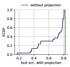
Figure 19: Results of the hyperparameter sweep of DPPL-Mean with projection.

For both methods, the utility with projection is always worse Figure 8 shows. The necessary accounting for the privacy costs of optimizing the additional hyperparameters [58] would further reduce the utility.

Appendix D Privacy Proofs and Privacy Conversion

D.1 Full Proof for Privacy Guarantees of DPPL-Public

We recall that our utility function is

$$u(\hat{\mathbf{x}},c)=\sum_{i=0}^{|\mathbf{X}_{c}|}1+\frac{\hat{M}(\mathbf{x}_{i})\cdot\hat{M}(\hat{\mathbf{x}})}{\lVert\hat{M}(\mathbf{x}_{i})\rVert\lVert\hat{M}(\hat{\mathbf{x}})\rVert}$$ (13)

where $\mathbf{X}_{c}\in\mathbf{X}$ are disjoint subsets of the private data $\mathbf{X}$ we want to keep private.

We choose $u$ to be the sum and not, for example, the mean of the cosine similarity, to make $u$ monotonic w.r.t. $\mathbf{X}$. It can be easily verified that the two different utility functions (mean and sum) lead to an identical mechanism, since the changes in $\Delta u$ and $u$ cancel each other out. As we exhaust the full range $[0,2]$ of the cosine similarities, we clip each similarity to $[d_{\text{min}},d_{\text{max}}]$ and then substract $d_{\text{min}}$. This gives us the adapted utility function

$$u(\hat{\mathbf{x}},c)=\sum_{i=0}^{|\mathbf{X}_{c}|}\text{clip}\left(1+\frac{\hat{M}(\mathbf{x}_{i})\cdot\hat{M}(\hat{\mathbf{x}})}{\lVert\hat{M}(\mathbf{x}_{i})\rVert\lVert\hat{M}(\hat{\mathbf{x}})\rVert},d_{\text{min}},d_{\text{max}}\right)-d_{\text{min}}$$ (14)

Lemma 5

$\Delta u=d_{\text{max}}-d_{\text{min}}$ and $u$ is positively monotonic w.r.t. to $\mathbf{X}$.

Proof. Since the cosine similarity’s range is bound to $[0,d_{\text{max}}-d_{\text{min}}]$, each private sample contributes one non-negative summand in $[0,d_{\text{max}}-d_{\text{min}}]$. It immediately follows that $\Delta u=d_{\text{max}}-d_{\text{min}}$ and $u$ is positively monotonic w.r.t. $\mathbf{X}$.

Theorem 2

DPPL-Public is $\varepsilon$-DP.

Proof. We sample the public prototypes independently for each class, using a utility function on disjoint sets $\mathbf{X}_{c}\in\mathbf{X}$ (each training data point only has one label), s.t. parallel composition applies. Each class prototype is sampled with the exponential mechanism, with probability $\Pr[\hat{\mathbf{x}}]\propto\exp{\left(\epsilon u_{(\hat{\mathbf{x}},c)}/\Delta u\right)}$ for outputting $\hat{\mathbf{x}}$ as the class prototype, with $\Delta u$ denoting the sensitivity of $u_{(\hat{\mathbf{x}},c)}$. Our utility function is monotonic (Lemma 5) and the described exponential mechanism is $\varepsilon$-DP for monotonic utility functions (Lemma 2). Since parallel composition applies and each parallel algorithm is $\varepsilon$-DP, the overall algorithm is $\varepsilon$-DP.

D.2 Comparing Between Different Notions of DP

Note that to fairly compare our developed method that yields pure DP guarantees against related work that yield zCDP, we convert our method using Lemma 3. To obtain a $\rho$-zCDP guarantee for the Linear Probing and DPSGD-Global-Adapt baselines, we perform full batch training and obtain the guarantee from Proposition 1.

Appendix E Additional Experimental Results

E.1 Imbalanced Experiments

ViT-B-16

ViT-L-16

ViT-H-14

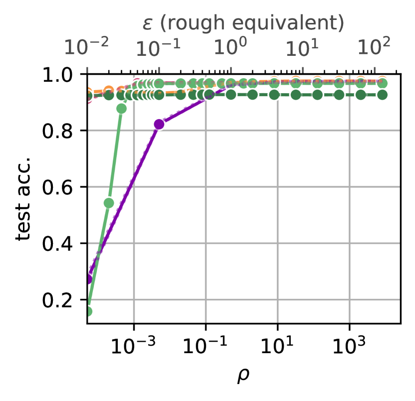
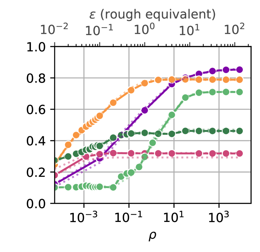
(b) IR=10.

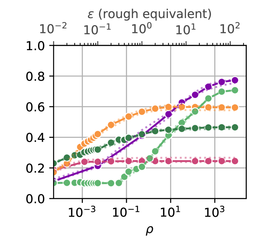
(c) IR=50.

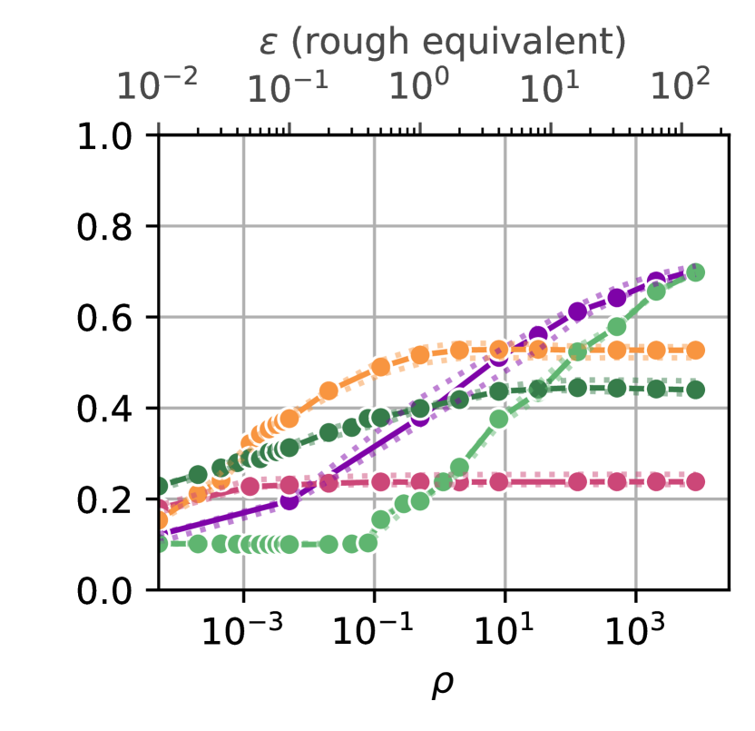
(d) IR=100.

Figure 20: DP Prototypes on CIFAR10. We present the results for CIFAR10 on ViT-B-16, ViT-H-14, ViT-L-16 and ResNet-50, using ImageNet as public data for DPPL-Public, at different levels of imbalance rations (IR). We compare to DP-LS by Mehta et al. [54] and DPSGD-Global-Adapt by Esipova et al. [29]. Plotted is the median over multiple runs and dotted lines represent the upper and lower quantiles for all methods.

ResNet-50

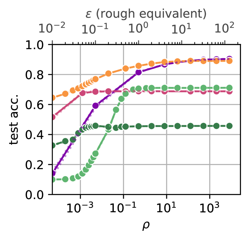
(a) IR=1.

ViT-B-16

ViT-L-16

ViT-H-14

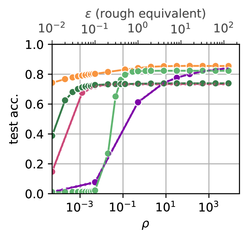
(b) IR=10.

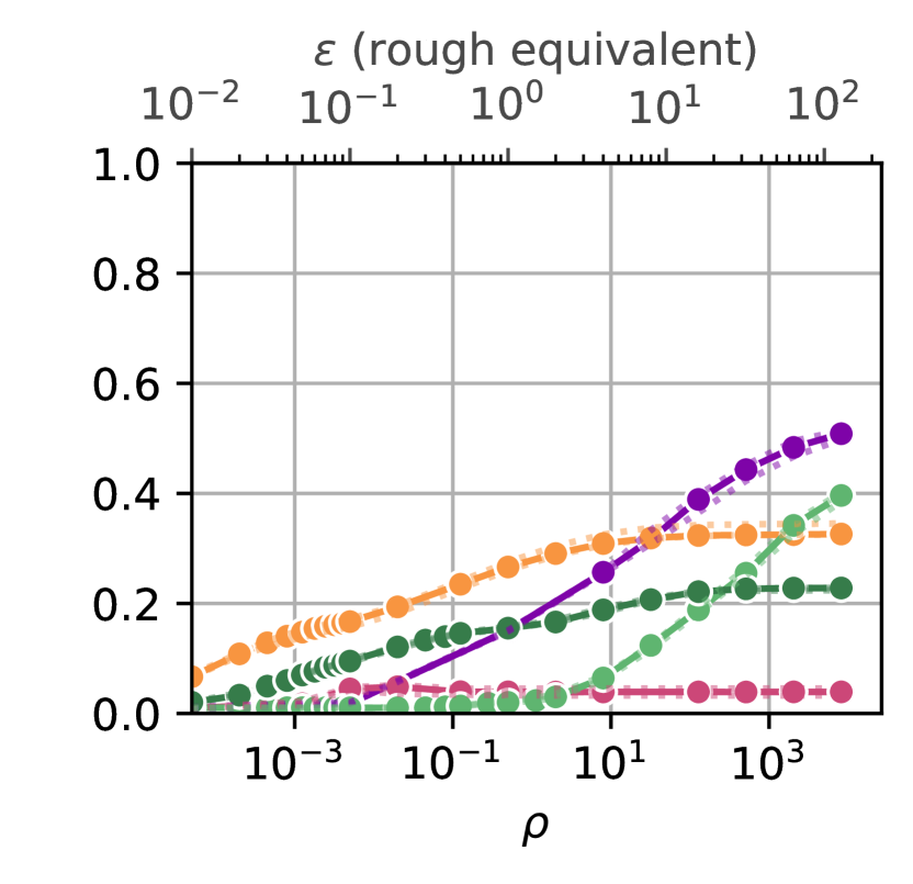
(c) IR=50.

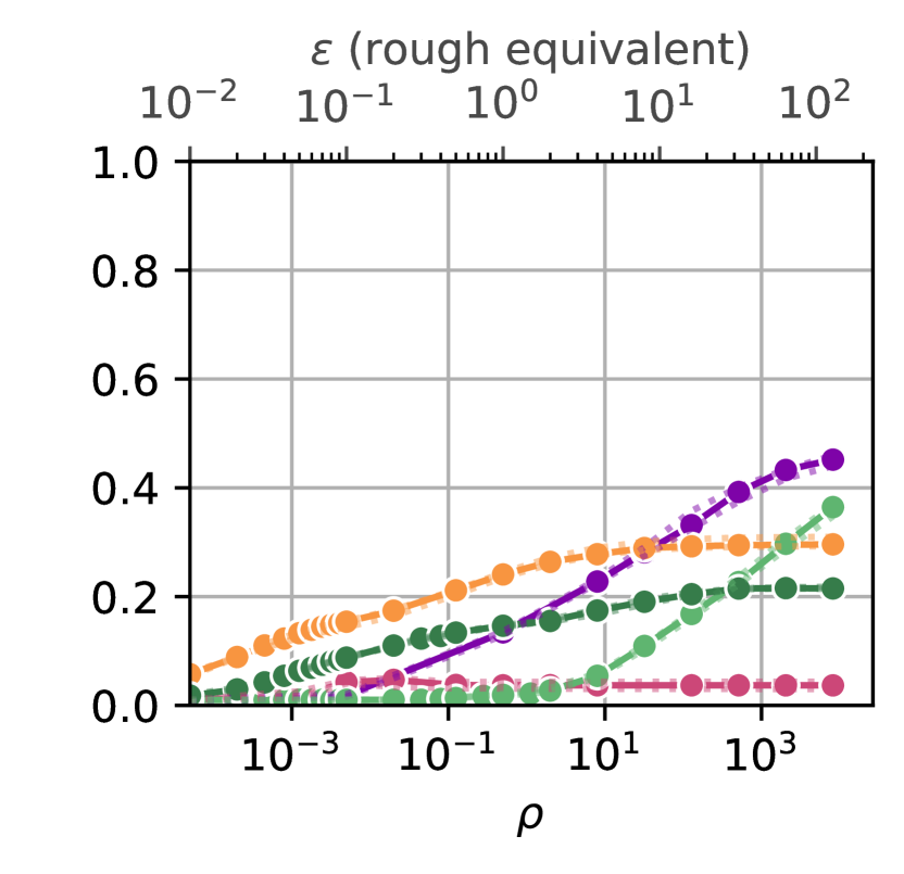
(d) IR=100.

Figure 21: DP Prototypes on CIFAR100. We present the results for CIFAR100 on ViT-B-16, ViT-H-14, ViT-L-16 and ResNet-50, using ImageNet as public data for DPPL-Public, at different levels of imbalance rations (IR). We compare to DP-LS by Mehta et al. [54] and DPSGD-Global-Adapt by Esipova et al. [29]. Plotted is the median over multiple runs and dotted lines represent the upper and lower quantiles for all methods.

ResNet-50

(a) IR=1.

ViT-B-16

ViT-L-16

ViT-H-14

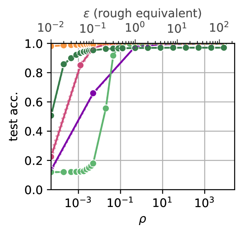
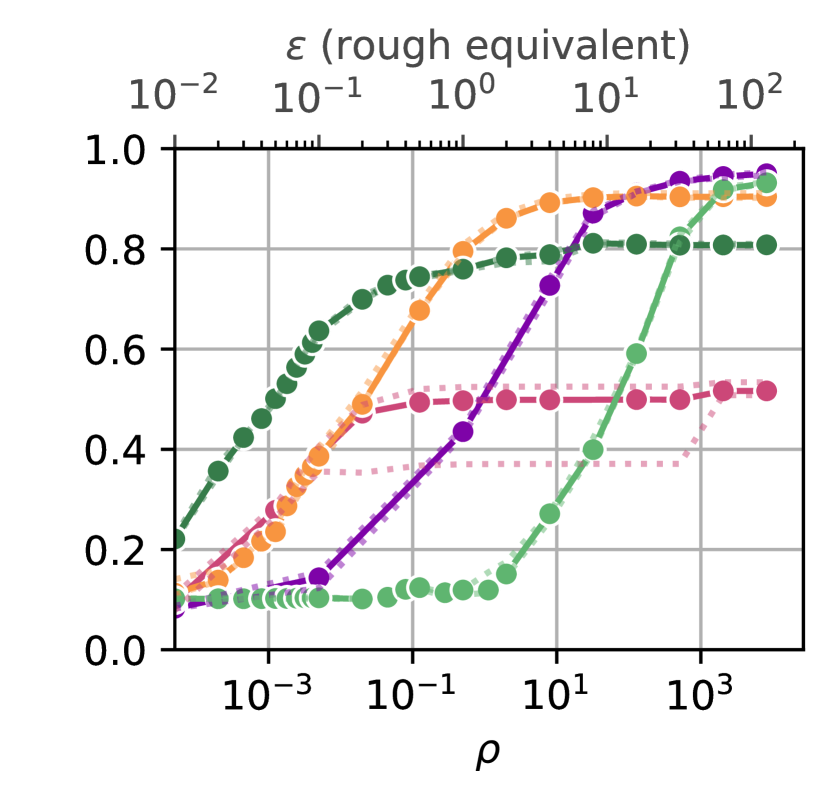
(b) IR=10.

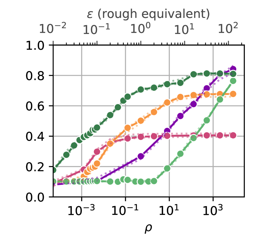
(c) IR=50.

(d) IR=100.

Figure 22: DP Prototypes on STL10. We present the results for STL10 on ViT-B-16, ViT-H-14, ViT-L-16 and ResNet-50, using ImageNet as public data for DPPL-Public, at different levels of imbalance rations (IR). We compare to DP-LS by Mehta et al. [54] and DPSGD-Global-Adapt by Esipova et al. [29]. Plotted is the median over multiple runs and dotted lines represent the upper and lower quantiles for all methods.

ResNet-50

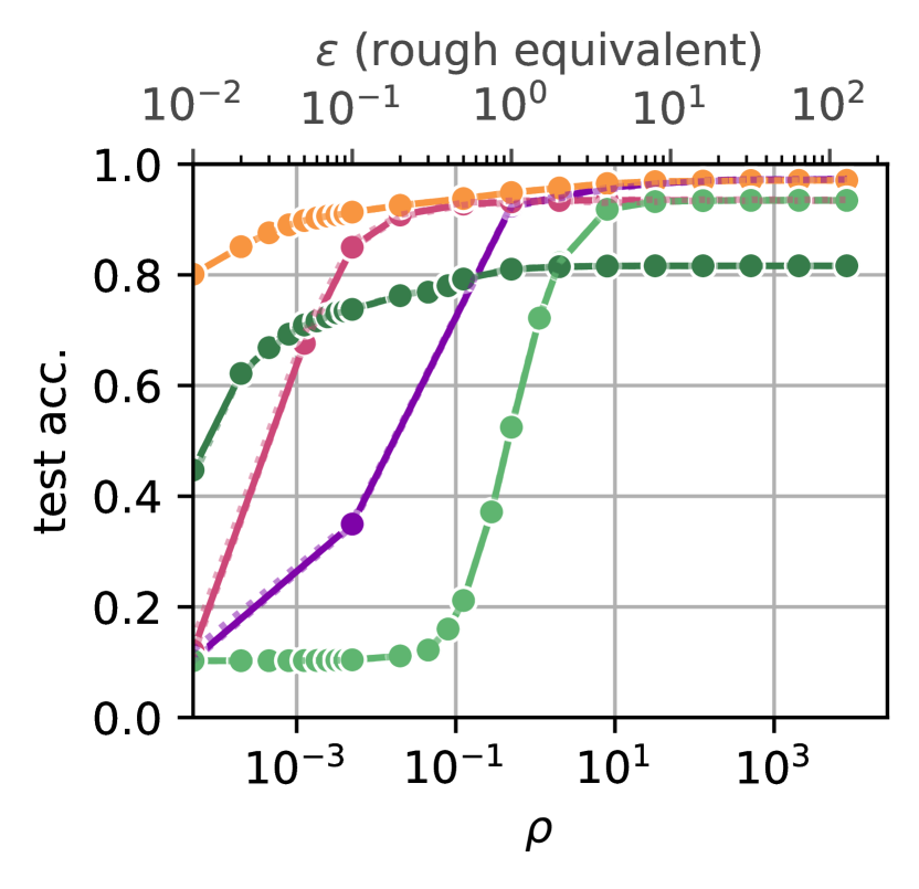
(a) IR=1.

ViT-B-16

ViT-L-16

ViT-H-14

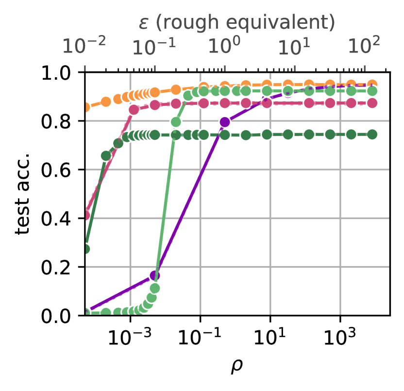
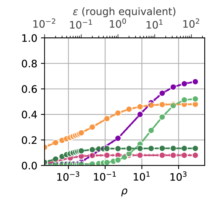
(b) IR=10.

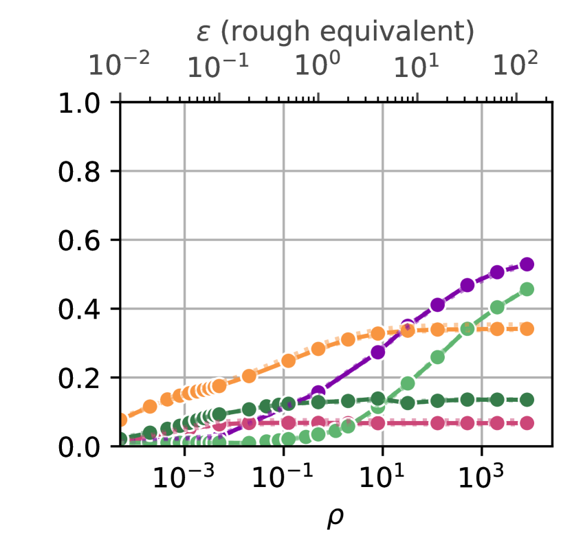
(c) IR=50.

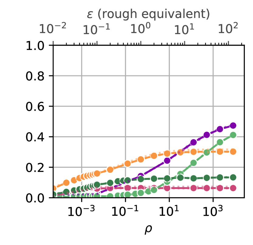
(d) IR=100.

Figure 23: DP Prototypes on FOOD101. We present the results for FOOD101 on ViT-B-16, ViT-H-14, ViT-L-16 and ResNet-50, using ImageNet as public data for DPPL-Public, at different levels of imbalance rations (IR). We compare to DP-LS by Mehta et al. [54] and DPSGD-Global-Adapt by Esipova et al. [29]. Plotted is the median over multiple runs and dotted lines represent the upper and lower quantiles for all methods.

ResNet-50

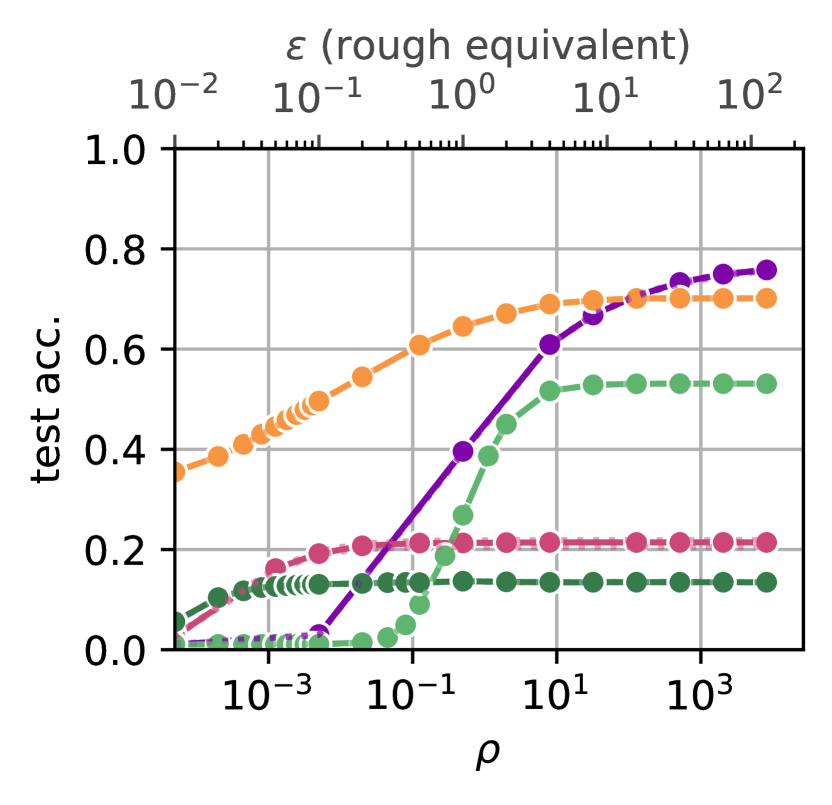
(a) IR=1.

We compare the accuracies for all methods, all encoders and imbalance ratios in $[1,10,50,100]$ in Figures 20, 22, 23 and 21.

E.2 Minority Class Accuracies

ViT-B-16

ViT-L-16

ViT-H-14

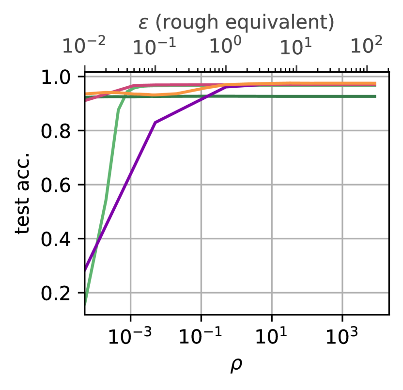
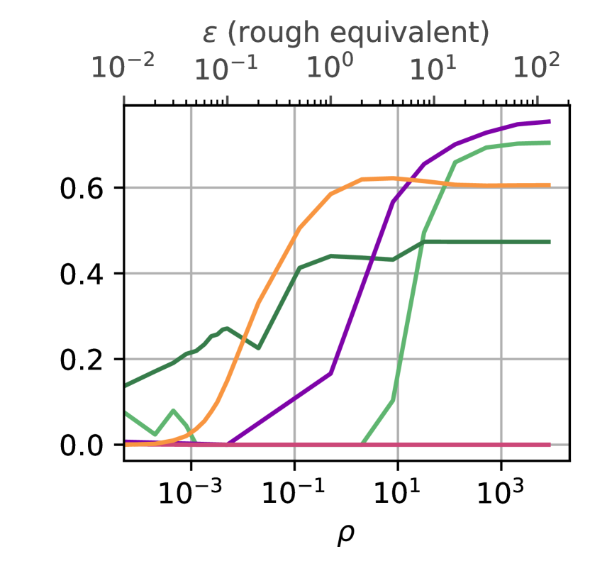
(b) IR=10.

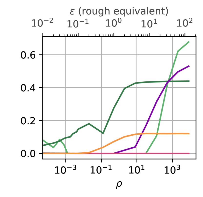
(c) IR=50.

(d) IR=100.

Figure 24: Minority class accuracies on CIFAR10. We present the results for the minority classes (lower 25% quantile) of CIFAR10 on ViT-B-16, ViT-H-14, ViT-L-16 and ResNet-50, using ImageNet as public data for DPPL-Public, at different levels of imbalance rations (IR). We compare to DP-LS by Mehta et al. [54] and DPSGD-Global-Adapt by Esipova et al. [29].

ResNet-50

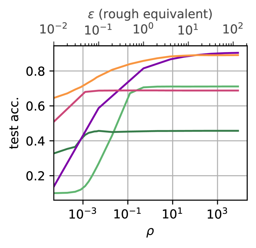
(a) IR=1.

ViT-B-16

ViT-L-16

ViT-H-14

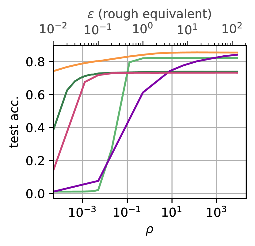
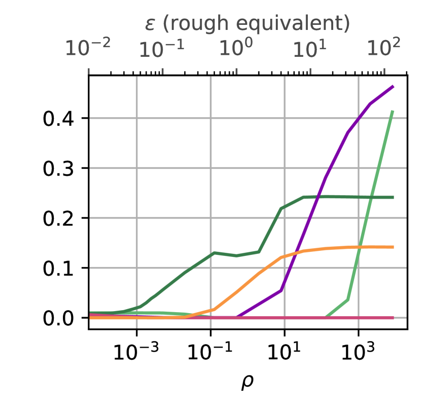
(b) IR=10.

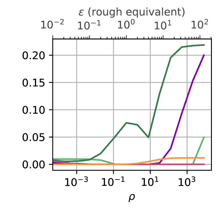
(c) IR=50.

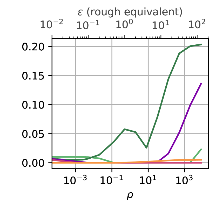
(d) IR=100.

Figure 25: Minority class accuracies on CIFAR100. We present the results for the minority classes (lower 25% quantile) of CIFAR100 on ViT-B-16, ViT-H-14, ViT-L-16 and ResNet-50, using ImageNet as public data for DPPL-Public, at different levels of imbalance rations (IR). We compare to DP-LS by Mehta et al. [54] and DPSGD-Global-Adapt by Esipova et al. [29].

ResNet-50

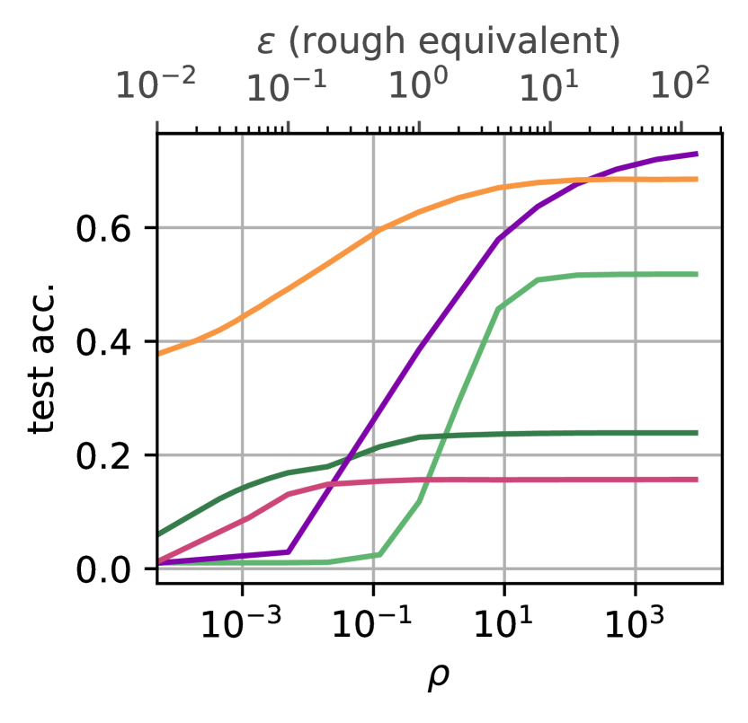
(a) IR=1.

ViT-B-16

ViT-L-16

ViT-H-14

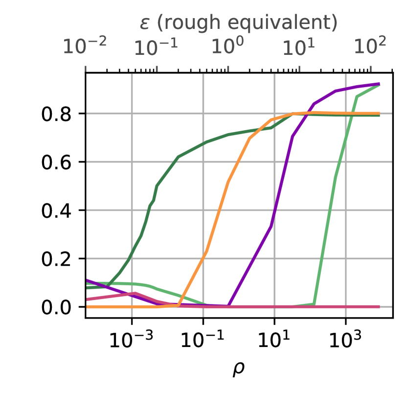
(b) IR=10.

(c) IR=50.

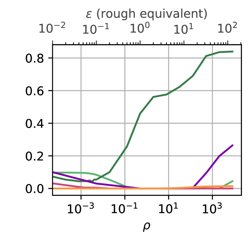
(d) IR=100.

Figure 26: Minority class accuracies on STL10. We present the results for the minority classes (lower 25% quantile) of STL10 on ViT-B-16, ViT-H-14, ViT-L-16 and ResNet-50, using ImageNet as public data for DPPL-Public, at different levels of imbalance rations (IR). We compare to DP-LS by Mehta et al. [54] and DPSGD-Global-Adapt by Esipova et al. [29].

ResNet-50

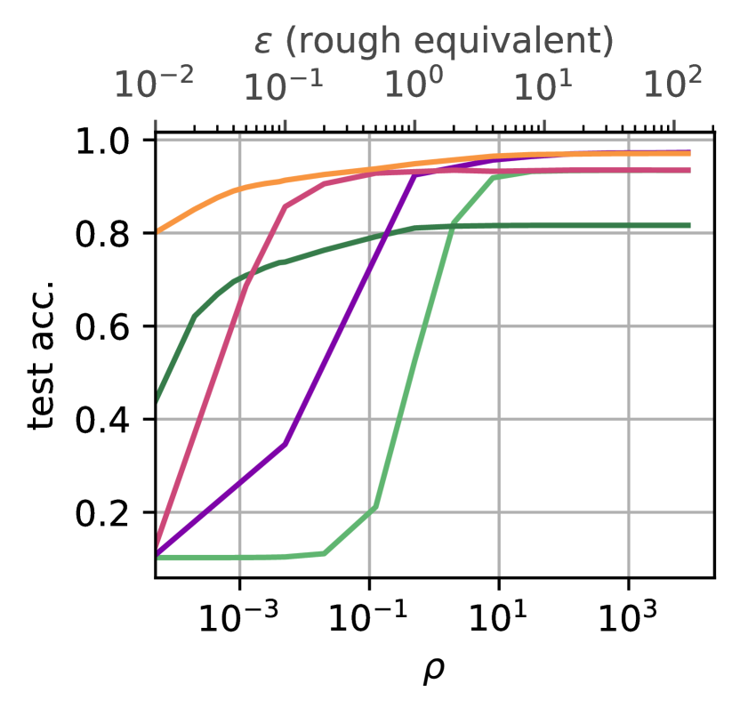
(a) IR=1.

ViT-B-16

ViT-L-16

ViT-H-14

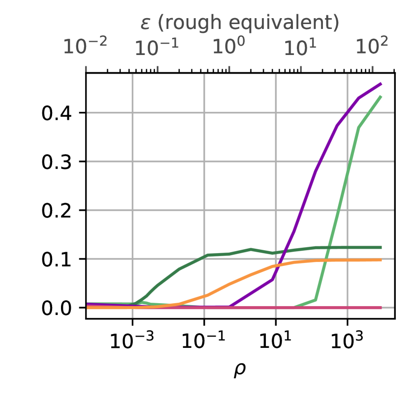
(b) IR=10.

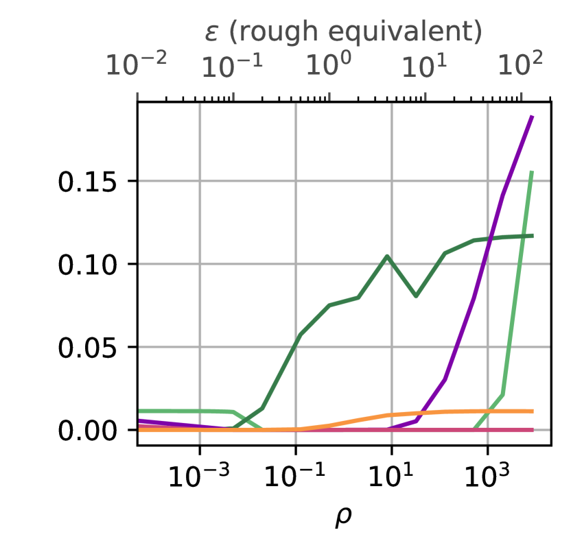
(c) IR=50.

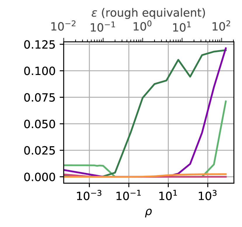
(d) IR=100.

Figure 27: Minority class accuracies on FOOD101. We present the results for the minority classes (lower 25% quantile) of FOOD101 on ViT-B-16, ViT-H-14, ViT-L-16 and ResNet-50, using ImageNet as public data for DPPL-Public, at different levels of imbalance rations (IR). We compare to DP-LS by Mehta et al. [54] and DPSGD-Global-Adapt by Esipova et al. [29].

ResNet-50

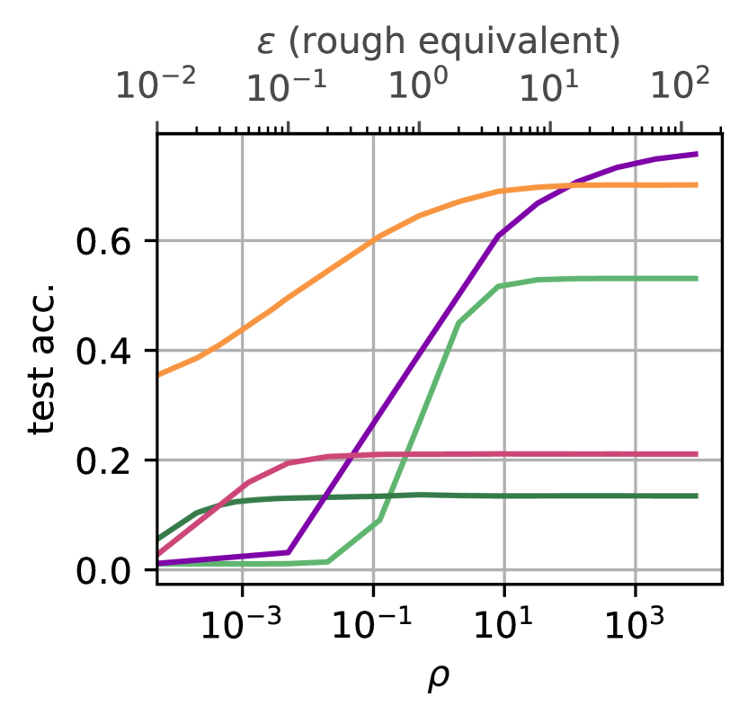
(a) IR=1.

We compare the accuracies of the minority classes for all methods, all encoders and imbalance ratios in $[1,10,50,100]$ in Figures 24, 26, 27 and 25.

E.3 Computational Runtimes

Table 2: Computational wall-time measurements of a single training on a single machine, limiting each method to a single GPU. Where applicable, iterative training was limited to 15 epochs. DPPL-Public’s score computation was conducted for 1,281,167 public samples.

	Step	Runtime [s]
		CIFAR10	CIFAR100
DPPL-Mean (Ours)	Mean Estimation	$0.079$	$0.168$
	Evaluation	$0.004$	$0.003$
DPPL-Public (Ours)	Utility Calculation	$5.0$	$34.3$
	Private Sampling	$0.0003$	$0.14$
	Evaluation	$0.010$	$0.013$
Linear Probing (DPSGD)	Iterative Training	$5.49$	$6.3$
	Evaluation	$0.060$	$0.066$
Esipova et al., 2023 (DPSGD-Global-Adapt)	Iterative Training	$174$	$242$
	Evaluation	$1.02$	$1.26$
Mehta et al., 2023 (DP-LS)	Setup	$0.49$	$2.2$
	Solving	$0.28$	$2.5$
	Evaluation	$0.058$	$0.11$

We compare the runtime for a single training in Table 2. We chose to compare CIFAR10 and CIFAR100 because the runtime of all methods scale with the number of classes on otherwise equally large training datasets.

Appendix F Discussion

F.1 Broader Impacts

We expect the prevalence of machine learning and it’s impact on society to ever increase. Our methods are especially useful at preserving the privacy of the training data, data that often consists of sensitive data from users. We consider contributing to an increase in the privacy of the training data and therefore protecting the users that contribute data to machine learning models to be a positive societal impact. Furthermore, our methods especially address the use case of imbalanced datasets. Real-world data is often long-tailed and models trained on unbalanced data can lead to unfair decisions w.r.t. to gender, ethnicity, disabilities, religion or social status, especially for minorities. We consider contributing to an improvement of the utility for minority classes as outlined in Figure 5 and Section E.2 to be a positive societal impact.

F.2 Limitations

We introduce DPPL as a novel approach to private transfer learning. Like all transfer learning methods, our method depends on a suitable base model. We’ve seen that especially ResNet-50 poses significant challenges, while the vision transformers worked well. The largest vision transformer ViT-H-14 yielded the best results of the compared models. We note that the combination of less suitable base models in addition to further out-of-distribution tasks, relative to the pre-training data, has a larger negative effect on the performance of our method compared to other methods. When evaluating the most out-of-distribution dataset, FOOD101, in combination with using embeddings from ResNet-50 or ViT-B-16, our methods are outperformed (see Figure 23. We can still claim the highest accuracy for minority classes in that case (see Figure 27), although the significance of that given the low utility is questionable. As we didn’t include the projection layer for our methods, the ability to adapt to these distribution shifts is limited and possibilities to include it need to be investigated further.

References

- Abadi et al. [2016] Martin Abadi, Andy Chu, Ian Goodfellow, H. Brendan McMahan, Ilya Mironov, Kunal Talwar, and Li Zhang. Deep Learning with Differential Privacy. In Proceedings of the 2016 ACM SIGSAC Conference on Computer and Communications Security, pages 308–318, Vienna Austria, October 2016. ACM. ISBN 978-1-4503-4139-4. doi: 10.1145/2976749.2978318. URL https://dl.acm.org/doi/10.1145/2976749.2978318.
- Akiba et al. [2019] Takuya Akiba, Shotaro Sano, Toshihiko Yanase, Takeru Ohta, and Masanori Koyama. Optuna: A Next-generation Hyperparameter Optimization Framework. In Proceedings of the 25th ACM SIGKDD International Conference on Knowledge Discovery & Data Mining, KDD ’19, pages 2623–2631, New York, NY, USA, July 2019. Association for Computing Machinery. ISBN 978-1-4503-6201-6. doi: 10.1145/3292500.3330701. URL https://doi.org/10.1145/3292500.3330701.
- Bagdasaryan et al. [2019] Eugene Bagdasaryan, Omid Poursaeed, and Vitaly Shmatikov. Differential Privacy Has Disparate Impact on Model Accuracy. Advances in Neural Information Processing Systems, 32, 2019. URL https://proceedings.neurips.cc/paper/2019/hash/fc0de4e0396fff257ea362983c2dda5a-Abstract.html?ref=https://githubhelp.com.
- Ben-David et al. [2024] Shai Ben-David, Alex Bie, Clément L Canonne, Gautam Kamath, and Vikrant Singhal. Private distribution learning with public data: The view from sample compression. Advances in Neural Information Processing Systems, 36, 2024.
- Bergstra et al. [2011] James Bergstra, Rémi Bardenet, Yoshua Bengio, and Balázs Kégl. Algorithms for Hyper-Parameter Optimization. In Advances in Neural Information Processing Systems, volume 24. Curran Associates, Inc., 2011. URL https://proceedings.neurips.cc/paper_files/paper/2011/hash/86e8f7ab32cfd12577bc2619bc635690-Abstract.html.
- Bie et al. [2022] Alex Bie, Gautam Kamath, and Vikrant Singhal. Private estimation with public data. Advances in neural information processing systems, 35:18653–18666, 2022.
- Biswas et al. [2020] Sourav Biswas, Yihe Dong, Gautam Kamath, and Jonathan Ullman. CoinPress: Practical Private Mean and Covariance Estimation. In Advances in Neural Information Processing Systems, volume 33, pages 14475–14485. Curran Associates, Inc., 2020. URL https://proceedings.neurips.cc/paper_files/paper/2020/hash/a684eceee76fc522773286a895bc8436-Abstract.html.
- Bossard et al. [2014] Lukas Bossard, Matthieu Guillaumin, and Luc Van Gool. Food-101 – Mining Discriminative Components with Random Forests. In David Fleet, Tomas Pajdla, Bernt Schiele, and Tinne Tuytelaars, editors, Computer Vision – ECCV 2014, pages 446–461, Cham, 2014. Springer International Publishing. ISBN 978-3-319-10599-4. doi: 10.1007/978-3-319-10599-4_29.
- Bradbury et al. [2018] James Bradbury, Roy Frostig, Peter Hawkins, Matthew James Johnson, Chris Leary, Dougal Maclaurin, George Necula, Adam Paszke, Jake VanderPlas, Skye Wanderman-Milne, and Qiao Zhang. JAX: composable transformations of Python+NumPy programs, 2018. URL http://github.com/google/jax.
- Bu et al. [2021] Zhiqi Bu, Sivakanth Gopi, Janardhan Kulkarni, Yin Tat Lee, Hanwen Shen, and Uthaipon Tantipongpipat. Fast and memory efficient differentially private-sgd via jl projections. Advances in Neural Information Processing Systems, 34:19680–19691, 2021.
- Bu et al. [2022] Zhiqi Bu, Jialin Mao, and Shiyun Xu. Scalable and efficient training of large convolutional neural networks with differential privacy. Advances in Neural Information Processing Systems, 35:38305–38318, 2022.
- Buda et al. [2018] Mateusz Buda, Atsuto Maki, and Maciej A Mazurowski. A systematic study of the class imbalance problem in convolutional neural networks. Neural networks, 106:249–259, 2018.
- Bun and Steinke [2016] Mark Bun and Thomas Steinke. Concentrated Differential Privacy: Simplifications, Extensions, and Lower Bounds. In Martin Hirt and Adam Smith, editors, Theory of Cryptography, Lecture Notes in Computer Science, pages 635–658, Berlin, Heidelberg, 2016. Springer. ISBN 978-3-662-53641-4. doi: 10.1007/978-3-662-53641-4_24.
- Cao et al. [2019] Kaidi Cao, Colin Wei, Adrien Gaidon, Nikos Arechiga, and Tengyu Ma. Learning Imbalanced Datasets with Label-Distribution-Aware Margin Loss. In Advances in Neural Information Processing Systems, volume 32. Curran Associates, Inc., 2019. URL https://proceedings.neurips.cc/paper/2019/hash/621461af90cadfdaf0e8d4cc25129f91-Abstract.html.
- Carlini et al. [2022] Nicholas Carlini, Steve Chien, Milad Nasr, Shuang Song, Andreas Terzis, and Florian Tramer. Membership inference attacks from first principles. In 2022 IEEE Symposium on Security and Privacy (SP), pages 1519–1519. IEEE Computer Society, 2022.
- Caron et al. [2021] Mathilde Caron, Hugo Touvron, Ishan Misra, Hervé Jégou, Julien Mairal, Piotr Bojanowski, and Armand Joulin. Emerging Properties in Self-Supervised Vision Transformers. In Proceedings of the IEEE/CVF International Conference on Computer Vision, pages 9650–9660, 2021. URL https://openaccess.thecvf.com/content/ICCV2021/html/Caron_Emerging_Properties_in_Self-Supervised_Vision_Transformers_ICCV_2021_paper.
- Cesar and Rogers [2021] Mark Cesar and Ryan Rogers. Bounding, Concentrating, and Truncating: Unifying Privacy Loss Composition for Data Analytics. In Proceedings of the 32nd International Conference on Algorithmic Learning Theory, pages 421–457. PMLR, March 2021. URL https://proceedings.mlr.press/v132/cesar21a.html. ISSN: 2640-3498.
- Chawla et al. [2002] N. V. Chawla, K. W. Bowyer, L. O. Hall, and W. P. Kegelmeyer. SMOTE: Synthetic Minority Over-sampling Technique. Journal of Artificial Intelligence Research, 16:321–357, June 2002. ISSN 1076-9757. doi: 10.1613/jair.953. URL https://www.jair.org/index.php/jair/article/view/10302.
- Coates et al. [2011] Adam Coates, Andrew Ng, and Honglak Lee. An Analysis of Single-Layer Networks in Unsupervised Feature Learning. In Proceedings of the Fourteenth International Conference on Artificial Intelligence and Statistics, pages 215–223. JMLR Workshop and Conference Proceedings, June 2011. URL https://proceedings.mlr.press/v15/coates11a.html. ISSN: 1938-7228.
- Cui et al. [2019] Yin Cui, Menglin Jia, Tsung-Yi Lin, Yang Song, and Serge Belongie. Class-Balanced Loss Based on Effective Number of Samples. pages 9268–9277, 2019. URL https://proceedings.neurips.cc/paper/2019/hash/621461af90cadfdaf0e8d4cc25129f91-Abstract.html.
- De et al. [2022] Soham De, Leonard Berrada, Jamie Hayes, Samuel L Smith, and Borja Balle. Unlocking high-accuracy differentially private image classification through scale. arXiv preprint arXiv:2204.13650, 2022.
- Deng et al. [2009] Jia Deng, Wei Dong, Richard Socher, Li-Jia Li, Kai Li, and Li Fei-Fei. ImageNet: A large-scale hierarchical image database. In 2009 IEEE Conference on Computer Vision and Pattern Recognition, pages 248–255, June 2009. doi: 10.1109/CVPR.2009.5206848. URL https://ieeexplore.ieee.org/abstract/document/5206848. ISSN: 1063-6919.
- [23] P Domingos. A general method for making classifiers cost-sensitive. Artificial Inelligence Group, Instituto Superior Técnico, Lisboa, pages 1049–001.
- Dong et al. [2019] Jinshuo Dong, Aaron Roth, and Weijie J. Su. Gaussian Differential Privacy, May 2019. URL http://arxiv.org/abs/1905.02383. arXiv:1905.02383 [cs, stat].
- Dong et al. [2020] Jinshuo Dong, David Durfee, and Ryan Rogers. Optimal Differential Privacy Composition for Exponential Mechanisms. In Proceedings of the 37th International Conference on Machine Learning, pages 2597–2606. PMLR, November 2020. URL https://proceedings.mlr.press/v119/dong20a.html. ISSN: 2640-3498.
- Dosovitskiy et al. [2020] Alexey Dosovitskiy, Lucas Beyer, Alexander Kolesnikov, Dirk Weissenborn, Xiaohua Zhai, Thomas Unterthiner, Mostafa Dehghani, Matthias Minderer, Georg Heigold, Sylvain Gelly, Jakob Uszkoreit, and Neil Houlsby. An Image is Worth 16x16 Words: Transformers for Image Recognition at Scale. In International Conference on Learning Representations, October 2020. URL https://openreview.net/forum?id=YicbFdNTTy&utm_campaign=f86497ed3a-EMAIL_CAMPAIGN_2019_04_24_03_18_COPY_01&utm_medium=email&utm_source=Deep%20Learning%20Weekly&utm_term=0_384567b42d-f86497ed3a-72965345.
- Durfee and Rogers [2019] David Durfee and Ryan M Rogers. Practical Differentially Private Top-k Selection with Pay-what-you-get Composition. In Advances in Neural Information Processing Systems, volume 32. Curran Associates, Inc., 2019. URL https://proceedings.neurips.cc/paper/2019/hash/b139e104214a08ae3f2ebcce149cdf6e-Abstract.html.
- Dwork et al. [2006] Cynthia Dwork, Frank McSherry, Kobbi Nissim, and Adam Smith. Calibrating Noise to Sensitivity in Private Data Analysis. In Shai Halevi and Tal Rabin, editors, Theory of Cryptography, Lecture Notes in Computer Science, pages 265–284, Berlin, Heidelberg, 2006. Springer. ISBN 978-3-540-32732-5. doi: 10.1007/11681878_14.
- Esipova et al. [2023] Maria S. Esipova, Atiyeh Ashari Ghomi, Yaqiao Luo, and Jesse C Cresswell. Disparate impact in differential privacy from gradient misalignment. In The eleventh international conference on learning representations, 2023. URL https://openreview.net/forum?id=qLOaeRvteqbx.
- Feldman [2020] Vitaly Feldman. Does learning require memorization? a short tale about a long tail. In Proceedings of the 52nd Annual ACM SIGACT Symposium on Theory of Computing, pages 954–959, Chicago IL USA, June 2020. ACM. ISBN 978-1-4503-6979-4. doi: 10.1145/3357713.3384290. URL https://dl.acm.org/doi/10.1145/3357713.3384290.
- Fredrikson et al. [2015] Matt Fredrikson, Somesh Jha, and Thomas Ristenpart. Model inversion attacks that exploit confidence information and basic countermeasures. In Proceedings of the 22nd ACM SIGSAC conference on computer and communications security, pages 1322–1333, 2015.
- Ganesh et al. [2023] Arun Ganesh, Mahdi Haghifam, Milad Nasr, Sewoong Oh, Thomas Steinke, Om Thakkar, Abhradeep Guha Thakurta, and Lun Wang. Why is public pretraining necessary for private model training? In International Conference on Machine Learning, pages 10611–10627. PMLR, 2023.
- Gillenwater et al. [2022] Jennifer Gillenwater, Matthew Joseph, Andres Munoz, and Monica Ribero Diaz. A Joint Exponential Mechanism For Differentially Private Top-$k$. In Proceedings of the 39th International Conference on Machine Learning, pages 7570–7582. PMLR, June 2022. URL https://proceedings.mlr.press/v162/gillenwater22a.html. ISSN: 2640-3498.
- Gu et al. [2022] Xin Gu, Gautam Kamath, and Steven Wu. Choosing public datasets for private machine learning via gradient subspace distance. In NeurIPS 2022 Workshop on Distribution Shifts: Connecting Methods and Applications, 2022.
- He et al. [2022a] Jiyan He, Xuechen Li, Da Yu, Huishuai Zhang, Janardhan Kulkarni, Yin Tat Lee, Arturs Backurs, Nenghai Yu, and Jiang Bian. Exploring the limits of differentially private deep learning with group-wise clipping. In The Eleventh International Conference on Learning Representations, 2022a.
- He et al. [2016] Kaiming He, Xiangyu Zhang, Shaoqing Ren, and Jian Sun. Deep Residual Learning for Image Recognition. pages 770–778, 2016. URL https://openaccess.thecvf.com/content_cvpr_2016/html/He_Deep_Residual_Learning_CVPR_2016_paper.html.
- He et al. [2022b] Kaiming He, Xinlei Chen, Saining Xie, Yanghao Li, Piotr Dollár, and Ross Girshick. Masked autoencoders are scalable vision learners. In Proceedings of the IEEE/CVF conference on computer vision and pattern recognition, pages 16000–16009, 2022b.
- Houlsby et al. [2019] Neil Houlsby, Andrei Giurgiu, Stanislaw Jastrzebski, Bruna Morrone, Quentin De Laroussilhe, Andrea Gesmundo, Mona Attariyan, and Sylvain Gelly. Parameter-efficient transfer learning for nlp. In International conference on machine learning, pages 2790–2799. PMLR, 2019.
- Hu et al. [2021] Edward J Hu, Phillip Wallis, Zeyuan Allen-Zhu, Yuanzhi Li, Shean Wang, Lu Wang, Weizhu Chen, et al. Lora: Low-rank adaptation of large language models. In International Conference on Learning Representations, 2021.
- Jagielski et al. [2019] Matthew Jagielski, Michael Kearns, Jieming Mao, Alina Oprea, Aaron Roth, Saeed Sharifi Malvajerdi, and Jonathan Ullman. Differentially Private Fair Learning. In Proceedings of the 36th International Conference on Machine Learning, pages 3000–3008. PMLR, May 2019. URL https://proceedings.mlr.press/v97/jagielski19a.html. ISSN: 2640-3498.
- [41] Nathalie Japkowicz. The Class Imbalance Problem: Signi cance and Strategies.
- Kamath and Ullman [2020] Gautam Kamath and Jonathan Ullman. A Primer on Private Statistics, April 2020. URL http://arxiv.org/abs/2005.00010. arXiv:2005.00010 [cs, math, stat].
- Krizhevsky [2009] Alex Krizhevsky. Learning Multiple Layers of Features from Tiny Images. 2009.
- Kubat et al. [1997] Miroslav Kubat, Stan Matwin, et al. Addressing the curse of imbalanced training sets: one-sided selection. In Icml, volume 97, page 179. Citeseer, 1997.
- Lee and Kifer [2021] Jaewoo Lee and Daniel Kifer. Scaling up differentially private deep learning with fast per-example gradient clipping. Proceedings on Privacy Enhancing Technologies, 2021.
- Lewis and Catlett [1994] David D. Lewis and Jason Catlett. Heterogeneous Uncertainty Sampling for Supervised Learning. In William W. Cohen and Haym Hirsh, editors, Machine Learning Proceedings 1994, pages 148–156. Morgan Kaufmann, San Francisco (CA), January 1994. ISBN 978-1-55860-335-6. doi: 10.1016/B978-1-55860-335-6.50026-X. URL https://www.sciencedirect.com/science/article/pii/B978155860335650026X.
- Li et al. [2021] Xuechen Li, Florian Tramer, Percy Liang, and Tatsunori Hashimoto. Large language models can be strong differentially private learners. arXiv preprint arXiv:2110.05679, 2021.
- Li et al. [2023] Yizhe Li, Yu-Lin Tsai, Chia-Mu Yu, Pin-Yu Chen, and Xuebin Ren. Exploring the benefits of visual prompting in differential privacy. In Proceedings of the IEEE/CVF International Conference on Computer Vision, pages 5158–5167, 2023.
- Ling and Li [1998] Charles X Ling and Chenghui Li. Data mining for direct marketing: Problems and solutions. In Kdd, volume 98, pages 73–79, 1998.
- Liu et al. [2019] Ziwei Liu, Zhongqi Miao, Xiaohang Zhan, Jiayun Wang, Boqing Gong, and Stella X Yu. Large-scale long-tailed recognition in an open world. In Proceedings of the IEEE/CVF conference on computer vision and pattern recognition, pages 2537–2546, 2019.
- McSherry and Talwar [2007] Frank McSherry and Kunal Talwar. Mechanism design via differential privacy. In 48th Annual IEEE Symposium on Foundations of Computer Science (FOCS’07), pages 94–103. IEEE, 2007.
- Medina and Gillenwater [2021] Andrés Muñoz Medina and Jenny Gillenwater. Duff: A Dataset-Distance-Based Utility Function Family for the Exponential Mechanism, January 2021. URL http://arxiv.org/abs/2010.04235. arXiv:2010.04235 [cs].
- Mehta et al. [2022] Harsh Mehta, Abhradeep Thakurta, Alexey Kurakin, and Ashok Cutkosky. Large Scale Transfer Learning for Differentially Private Image Classification, May 2022. URL http://arxiv.org/abs/2205.02973. arXiv:2205.02973 [cs].
- Mehta et al. [2023] Harsh Mehta, Walid Krichene, Abhradeep Guha Thakurta, Alexey Kurakin, and Ashok Cutkosky. Differentially private image classification from features. Transactions on Machine Learning Research, 2023. ISSN 2835-8856. URL https://openreview.net/forum?id=Cj6pLclmwT.
- Mironov [2017] Ilya Mironov. Rényi Differential Privacy. In 2017 IEEE 30th Computer Security Foundations Symposium (CSF), pages 263–275, Santa Barbara, CA, August 2017. IEEE. ISBN 978-1-5386-3217-8. doi: 10.1109/CSF.2017.11. URL https://ieeexplore.ieee.org/document/8049725/.
- Moritz et al. [2018] Philipp Moritz, Robert Nishihara, Stephanie Wang, Alexey Tumanov, Richard Liaw, Eric Liang, Melih Elibol, Zongheng Yang, William Paul, Michael I. Jordan, and Ion Stoica. Ray: A Distributed Framework for Emerging {AI} Applications. pages 561–577, 2018. ISBN 978-1-939133-08-3. URL https://www.usenix.org/conference/osdi18/presentation/moritz.
- Oquab et al. [2023] Maxime Oquab, Timothée Darcet, Théo Moutakanni, Huy Vo, Marc Szafraniec, Vasil Khalidov, Pierre Fernandez, Daniel Haziza, Francisco Massa, Alaaeldin El-Nouby, Mahmoud Assran, Nicolas Ballas, Wojciech Galuba, Russell Howes, Po-Yao Huang, Shang-Wen Li, Ishan Misra, Michael Rabbat, Vasu Sharma, Gabriel Synnaeve, Hu Xu, Hervé Jegou, Julien Mairal, Patrick Labatut, Armand Joulin, and Piotr Bojanowski. DINOv2: Learning Robust Visual Features without Supervision, April 2023. URL http://arxiv.org/abs/2304.07193. arXiv:2304.07193 [cs].
- Papernot and Steinke [2021] Nicolas Papernot and Thomas Steinke. Hyperparameter tuning with renyi differential privacy. arXiv preprint arXiv:2110.03620, 2021.
- Papernot et al. [2017] Nicolas Papernot, Martín Abadi, Úlfar Erlingsson, Ian Goodfellow, and Kunal Talwar. Semi-supervised knowledge transfer for deep learning from private training data. In Proceedings of the International Conference on Learning Representations, 2017. URL https://arxiv.org/abs/1610.05755.
- Papernot et al. [2018] Nicolas Papernot, Shuang Song, Ilya Mironov, Ananth Raghunathan, Kunal Talwar, and Úlfar Erlingsson. Scalable private learning with pate. In International Conference on Learning Representations (ICLR), 2018. URL https://arxiv.org/abs/1802.08908.
- Paszke et al. [2019] Adam Paszke, Sam Gross, Francisco Massa, Adam Lerer, James Bradbury, Gregory Chanan, Trevor Killeen, Zeming Lin, Natalia Gimelshein, Luca Antiga, Alban Desmaison, Andreas Kopf, Edward Yang, Zachary DeVito, Martin Raison, Alykhan Tejani, Sasank Chilamkurthy, Benoit Steiner, Lu Fang, Junjie Bai, and Soumith Chintala. PyTorch: An Imperative Style, High-Performance Deep Learning Library. In Advances in Neural Information Processing Systems, volume 32. Curran Associates, Inc., 2019. URL https://proceedings.neurips.cc/paper/2019/hash/bdbca288fee7f92f2bfa9f7012727740-Abstract.html.
- Radford et al. [2021] Alec Radford, Jong Wook Kim, Chris Hallacy, Aditya Ramesh, Gabriel Goh, Sandhini Agarwal, Girish Sastry, Amanda Askell, Pamela Mishkin, Jack Clark, et al. Learning transferable visual models from natural language supervision. In International conference on machine learning, pages 8748–8763. PMLR, 2021.
- Reed [2001] William J Reed. The pareto, zipf and other power laws. Economics letters, 74(1):15–19, 2001.
- Rocklin [2015] Matthew Rocklin. Dask: Parallel Computation with Blocked algorithms and Task Scheduling. In SciPy, pages 126–132, Austin, Texas, 2015. doi: 10.25080/Majora-7b98e3ed-013. URL https://conference.scipy.org/proceedings/scipy2015/matthew_rocklin.html.
- Sharma et al. [2018] Piyush Sharma, Nan Ding, Sebastian Goodman, and Radu Soricut. Conceptual Captions: A Cleaned, Hypernymed, Image Alt-text Dataset For Automatic Image Captioning. In Iryna Gurevych and Yusuke Miyao, editors, Proceedings of the 56th Annual Meeting of the Association for Computational Linguistics (Volume 1: Long Papers), pages 2556–2565, Melbourne, Australia, July 2018. Association for Computational Linguistics. doi: 10.18653/v1/P18-1238. URL https://aclanthology.org/P18-1238.
- Shokri et al. [2017] Reza Shokri, Marco Stronati, Congzheng Song, and Vitaly Shmatikov. Membership inference attacks against machine learning models. In 2017 IEEE symposium on security and privacy (SP), pages 3–18. IEEE, 2017.
- Singh et al. [2022] Mannat Singh, Laura Gustafson, Aaron Adcock, Vinicius de Freitas Reis, Bugra Gedik, Raj Prateek Kosaraju, Dhruv Mahajan, Ross Girshick, Piotr Dollár, and Laurens van der Maaten. Revisiting Weakly Supervised Pre-Training of Visual Perception Models. In Proceedings of the IEEE/CVF Conference on Computer Vision and Pattern Recognition, pages 804–814, 2022. URL https://openaccess.thecvf.com/content/CVPR2022/html/Singh_Revisiting_Weakly_Supervised_Pre-Training_of_Visual_Perception_Models_CVPR_2022_paper.html.
- Snell et al. [2017] Jake Snell, Kevin Swersky, and Richard Zemel. Prototypical Networks for Few-shot Learning. In Advances in Neural Information Processing Systems, volume 30. Curran Associates, Inc., 2017. URL https://proceedings.neurips.cc/paper_files/paper/2017/hash/cb8da6767461f2812ae4290eac7cbc42-Abstract.html.
- Song et al. [2022] Qi Song, Zebin Peng, Luchen Ji, Xiaochen Yang, and Xiaoxu Li. Dual Prototypical Network for Robust Few-shot Image Classification. In 2022 Asia-Pacific Signal and Information Processing Association Annual Summit and Conference (APSIPA ASC), pages 533–537, Chiang Mai, Thailand, November 2022. IEEE. ISBN 978-616-590-477-3. doi: 10.23919/APSIPAASC55919.2022.9979898. URL https://ieeexplore.ieee.org/document/9979898/.
- Song et al. [2013] Shuang Song, Kamalika Chaudhuri, and Anand D Sarwate. Stochastic gradient descent with differentially private updates. In 2013 IEEE global conference on signal and information processing, pages 245–248. IEEE, 2013.
- Subramani et al. [2021] Pranav Subramani, Nicholas Vadivelu, and Gautam Kamath. Enabling fast differentially private sgd via just-in-time compilation and vectorization. Advances in Neural Information Processing Systems, 34:26409–26421, 2021.
- Suriyakumar et al. [2021] Vinith M Suriyakumar, Nicolas Papernot, Anna Goldenberg, and Marzyeh Ghassemi. Chasing your long tails: Differentially private prediction in health care settings. In Proceedings of the 2021 ACM Conference on Fairness, Accountability, and Transparency, pages 723–734, 2021.
- Tramèr et al. [2022] Florian Tramèr, Gautam Kamath, and Nicholas Carlini. Considerations for differentially private learning with large-scale public pretraining. arXiv preprint arXiv:2212.06470, 2022.
- Tsfadia et al. [2022] Eliad Tsfadia, Edith Cohen, Haim Kaplan, Yishay Mansour, and Uri Stemmer. FriendlyCore: Practical Differentially Private Aggregation. In Proceedings of the 39th International Conference on Machine Learning, pages 21828–21863. PMLR, June 2022. URL https://proceedings.mlr.press/v162/tsfadia22a.html. ISSN: 2640-3498.
- Wang et al. [2019] Yu-Xiang Wang, Borja Balle, and Shiva Prasad Kasiviswanathan. Subsampled Renyi Differential Privacy and Analytical Moments Accountant. In Proceedings of the Twenty-Second International Conference on Artificial Intelligence and Statistics, pages 1226–1235. PMLR, April 2019. URL https://proceedings.mlr.press/v89/wang19b.html. ISSN: 2640-3498.
- Wang et al. [2018] Yu-Xiong Wang, Ross Girshick, Martial Hebert, and Bharath Hariharan. Low-Shot Learning from Imaginary Data. In 2018 IEEE/CVF Conference on Computer Vision and Pattern Recognition, pages 7278–7286, June 2018. doi: 10.1109/CVPR.2018.00760. URL https://ieeexplore.ieee.org/abstract/document/8578858. ISSN: 2575-7075.
- Yadan [2019] Omry Yadan. Hydra - a framework for elegantly configuring complex applications. Github, 2019. URL https://github.com/facebookresearch/hydra.
- Yousefpour et al. [2021] Ashkan Yousefpour, Igor Shilov, Alexandre Sablayrolles, Davide Testuggine, Karthik Prasad, Mani Malek, John Nguyen, Sayan Ghosh, Akash Bharadwaj, Jessica Zhao, Graham Cormode, and Ilya Mironov. Opacus: User-Friendly differential privacy library in PyTorch. arXiv preprint arXiv:2109.12298, 2021.
- Yu et al. [2021] Da Yu, Saurabh Naik, Arturs Backurs, Sivakanth Gopi, Huseyin A Inan, Gautam Kamath, Janardhan Kulkarni, Yin Tat Lee, Andre Manoel, Lukas Wutschitz, et al. Differentially private fine-tuning of language models. arXiv preprint arXiv:2110.06500, 2021.
- [80] Shiran Zada, Itay Benou, and Michal Irani. Pure Noise to the Rescue of Insufficient Data: Improving Imbalanced Classification by Training on Random Noise Images.
- Zhu and Wang [2019] Yuqing Zhu and Yu-Xiang Wang. Poission Subsampled Rényi Differential Privacy. In Proceedings of the 36th International Conference on Machine Learning, pages 7634–7642. PMLR, May 2019. URL https://proceedings.mlr.press/v97/zhu19c.html. ISSN: 2640-3498.