Quantifying the Uncertainty of Uncertainty - Extending Greenwood’s Formula to Variances
Biostatistics and Medical Biometry, Medical School OWL
Bielefeld University
Universitätsstr. 25
33615 Bielefeld
Germany &
Biostatistics and Medical Biometry, Medical School OWL
Bielefeld University
Universitätsstr. 25
33615 Bielefeld
Germany
Abstract
In this article, we introduce an estimator for the asymptotic variance of the Greenwood variance estimator, where the latter is crucial for assessing the accuracy of the Kaplan–Meier survival estimator. The result indicates that the asymptotic variance of the Greenwood variance estimator is considerably smaller than that of the Kaplan–Meier variance estimator. This finding emphasizes the robustness of the Greenwood estimator.
Keywords Asymptotic variance Delta method Greenwood estimator Kaplan–Meier estimator
1 Introduction
Quantifying uncertainty is one of the central tasks of statistics. But, quantification of uncertainty itself is subject to uncertainty. For example, the estimate of a variance naturally also has a variance, and an estimator of this variance provides information on the robustness of the original variance estimator. For non-parametric estimators of the survival function, research (Reid (1981)) has focused on estimating the asymptotic variance (denoted as A.Var in the following) of functionals (e.g. moments such as expected value and variance) of the Kaplan–Meier estimator. These results are derived using the functional delta method, leading to Riemann–Stieltjes integrals which are challenging to evaluate directly. Interpretation using Dirac delta distributions as generalized functions is necessary, and even then, the resulting integrals generally can only be resolved using numerical methods. Furthermore, the calculation requires knowledge of the influence function (Hampel (1974), Lambert (1981)) of the functional under consideration.
In this article, we focus on estimating the asymptotic variance of the asymptotic variance of the Kaplan–Meier estimator using the classical, i.e. function based, delta method rather than the functional delta method. The method is combined with a recursive estimation process applied to the Greenwood variance estimator. This approach allows us to derive a closed, directly computable estimator for the asymptotic variance of the asymptotic variance of the Kaplan–Meier estimator, which nicely resembles the original Greenwood estimator structurally.
The article is organized as follows.
We start with introducing the Kaplan–Meier estimator, denoted as .
The variance of , estimated using the Greenwood estimator, serves to quantify variability. This measure, defined as the asymptotic variance of , is of order . We then examine the asymptotic variance of the Greenwood estimator itself, which turns out to be of order .
After proving our main result, we apply our estimator to the LEADER Type 2 Diabetes Study (Marso et al., 2016) for demonstration purposes. We conclude with a discussion of our findings, including the limitations of our work and suggestions for future research in this field.
2 Kaplan–Meier Estimator and Greenwood Estimator
In the following, we will give some definitions used throughout the article.
Definition 1
Let denote the Kaplan–Meier estimator,
| (1) |
where are observation times (), the number of events and the number of people at risk immediately before time . Further,
| (2) |
denotes the corresponding hazard rate. Additionally, we let A.Var() denote the asymptotic variance of an estimator .
The variance of the Kaplan–Meier estimator can be asymptotically estimated and is known as Greenwood’s formula, denoted by (Greenwood (1926)).
Theorem 1
(Greenwood’s formula)
Let be the Kaplan–Meier estimator (1). Then the variance of can be asymptotically estimated by
| (3) |
3 Main Result: Variance of the the Greenwood Estimator
Consider the estimated asymptotic variance of the Kaplan–Meier estimator (1) given by the Greenwood estimator (3). Our aim is to to derive an asymptotic estimator
| (4) |
for the variance of the estimator . Our main result is:
Theorem 2
Corollary 1
Pointwise Wald-type confidence intervals at confidence level can be calculated using equation (5) by
| (6) |
where denotes the quantile function of the standard normal distribution.
Equation (6) holds true if is asymptotically normally distributed, which can be reasonably assumed because is normally distributed and equation
4 Proof of Main Result
Our proof of Theorem 2 comprises five steps. In Step 1, we constitute a fundamental initial estimate using the delta method, which describes a relationship between , the variance of , and the variance of . Steps 2 to 4 again use the delta method for further refinements of the fundamental estimate. These steps recursively ensure that only known quantities are included in the estimates. In the final step, the intermediate results are combined to obtain the desired final estimate (5). In the appendices, we provide the necessary auxiliary results for the estimates, along with their respective proofs.
4.1 Initial Estimate for the Asymptotic Variance of
From Equation (3) it follows that is a sum of random variables, which we assume to be (pointwise) independent and identically distributed (i.i.d.). Furthermore, we assume that these random variables have a common expected value and a common variance. Then, we can apply the central limit theorem (Appendix 1, Theorem 3) and conclude that is (pointwise) asymptotically normally distributed. Thus, the delta method (Appendix 1, Theorem 4) is applicable to with . This yields
and thus
| (7) |
We let
| (8) |
and estimate (8) in the next section.
4.2 Estimate for
Based on the representation given in Equation (3) for , it follows
where denotes the covariance term
Now, we can apply equation (25) from Lemma 1 (Appendix 2) to the second argument of . From this we obtain
Given that the asymptotic variance of is the variance of the asymptotic distribution of , we have
where is not a random variable, but a fixed real value. Consequently, we can conclude that asymptotically. Then, by using Equation (25) from Lemma 1 (Appendix 2) once more, we can further infer that
| (9) |
asymptotically. Now, we rewrite Equation (9) by
| (10) |
and estimate
| (11) |
in the next section.
4.3 Estimate for
The term
is a sum of random variables, which we again assume to be (pointwise) i.i.d. and to have a common expected value and variance. Then, according to the central limit theorem, it can be assumed that is (pointwise) asymptotically normally distributed. Consequently, the delta method can be applied to with transformation function :
It follows that
with covariance term
due to Lemma 1 (ii) (Appendix 2). Thus, we let
| (12) |
and estimate
| (13) |
for with in the next section.
4.4 Estimates for
For with we let
using (2). Assuming that are i.i.d. and have a common expected value and variance, we can apply the central limit theorem and subsequently employ the delta method to with . With we find:
| (14) | ||||
| (15) |
where equality (14) follows from Corollary 2 (iii) (Appendix 2) and equality (15) follows from Corollary 2 (i) (Appendix 2).
Finally, applying again, we conclude
| (16) |
4.5 Final Estimate for the Asymptotic Variance of
5 Application
In this section, we use the data set of the LEADER trial to demonstrate the computation of the asymptotic variance of the asymptocic variance of the corresponding Kaplan–Meier survival estimator (Marso et al., 2016). The dataset used here is a subset of the LEADER-study dataset describing the survival in patients with type 2 diabetes, providing information from the 9344 patients in the placebo group. Table 1 displays an extract of the dataset containing the pertinent variables for our analysis, where time denotes the survival time in years, and status indicates whether an observation was censored (status = 0) or not (status = 1).
| time | status | |
|---|---|---|
| 1 | 0.7276761 | 1 |
| 2 | 1.1432777 | 1 |
| 3 | 1.4698922 | 1 |
| 4 | 1.4698922 | 1 |
| 5 | 1.4698922 | 1 |
| 9344 | 54 | 0 |
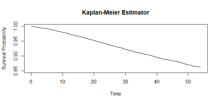
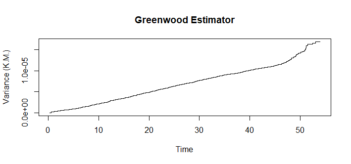
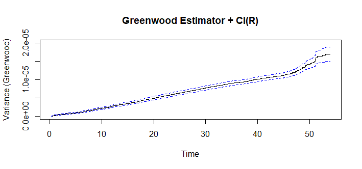
Based on the LEADER study data subset, figures 1 - 3 depict the Kaplan–Meier estimator (Fig. 1), the Greenwood estimator (Fig. 2) and the asymptotic variance estimator of the Greenwood estimator (Fig. 3). It becomes obvious that the survival probability decreases approximately linear over time. The corresponding variance calculated using the Greenwood estimator increases over time, but the order of magnitude is close to zero. The same applies to the estimator.
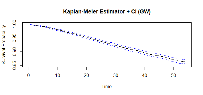
Figures 4 and 5 show the Kaplan–Meier estimator with pointwise 95% Wald-type confidence intervals (Fig. 4) and the Greenwood estimator with corresponding 95% pointwise Wald-type confidence intervals (6) (Fig. 5).

6 Discussion
In this article, we showed how the variance of the Greenwood estimator can be derived to quantify its uncertainty and to calculate corresponding Wald-type confidence intervals. Our starting point was the Kaplan–Meier estimator (Kaplan and Meier, 1958).
To assess the precision of the Kaplan–Meier estimator, it is essential to estimate its variance. The Greenwood estimator is commonly employed for this purpose. The Greenwood variance, denoted as , quantifies the variability of the Kaplan–Meier estimator by estimating it’s asymptotic variance. The asymptotic variance of is of order .
In addition to estimating the variance of the Kaplan–Meier estimator, it is also of interest to estimate the variance of the Greenwood estimator itself. This variance, denoted as , is of the order and consequently of the order . This estimator structurally resembles the Greenwood estimator: whereas the Greenwood estimator is a product of and a sum, the estimator similarly is a product of and a funtion of that sum.
Although our proof of Theorem 2 frequently utilizes the delta method, it is not a priori always clear in all estimates whether the data are such that the method is applicable. Moreover, verifying its applicability for given data generally proves to be quite challenging. In this context, our findings have limitations, which should be carefully considered when interpreting the results.
A promising focus for future research is the determination of the asymptotic variance of the Kaplan–Meier estimator’s variance. This can be achieved by rigorously applying the functional delta method approach, which would provide deeper insights into the estimator’s long-term behavior and potential applications. While the method introduced in this article estimates the asymptotic variance estimator of the asymptotic variance of the Kaplan–Meier estimator based on the Greenwood estimator, the functional delta method would estimate the asymptotic variance of the variance - rather than the asymptotic variance of the asymptotic variance - which theoretically yields a more precise variance estimator. Linking these theoretical insights with the practical application, the functional delta method approach could possibly refine our analytical capabilities.
References
- Reid [1981] N Reid. Influence functions for censored data. the annals of statistics 1981, vol 9, no 1, 78–92. 1981.
- Hampel [1974] Frank R Hampel. The influence curve and its role in robust estimation. Journal of the american statistical association, 69(346):383–393, 1974.
- Lambert [1981] Diane Lambert. Influence functions for testing. Journal of the American Statistical Association, 76(375):649–657, 1981.
- Marso et al. [2016] Steven P Marso, Gilbert H Daniels, Kirstine Brown-Frandsen, Peter Kristensen, Johannes FE Mann, Michael A Nauck, Steven E Nissen, Stuart Pocock, Neil R Poulter, Lasse S Ravn, et al. Liraglutide and cardiovascular outcomes in type 2 diabetes. New England Journal of Medicine, 375(4):311–322, 2016.
- Greenwood [1926] Major Greenwood. The natural duration of cancer (report on public health and medical subjects no 33). London: Stationery Office, 1926.
- Kaplan and Meier [1958] Edward L Kaplan and Paul Meier. Nonparametric estimation from incomplete observations. Journal of the American statistical association, 53(282):457–481, 1958.
- Rao [1973] C R Rao. Linear statistical inference and its applications, volume 2. Wiley New York, 1973.
- Schervish [2012] Mark J Schervish. Theory of statistics. Springer Science & Business Media, 2012.
- Witting [1995] U Witting, H Müller-Funk. Mathematische Statistik II. Teubner-Verlag, 1995.
- Cox and Oakes [1984] DR Cox and D Oakes. Analysis of survival data. Chapman and Hall, London, 1984.
- Hafner [2001] Robert Hafner. Nichtparametrische Verfahren der Statistik. Springer-Verlag, 2001.
Appendix 1
Fundamental theorems
We present two fundamental theorems of statistics that serve as the theoretical foundation required for the derivation of our main result.
Theorem 3
(Central limit theorem)
Let be a sequence of independent and identically distributed (i.i.d.) random variables with a common mean () and a common finite variance (). Then, as approaches infinity, the distribution of the sample mean () approaches a normal distribution with mean and variance ,
where is the cumulative distribution function of the standard normal distribution.
This theorem essentially states that the sum (or average) of a large number of independent and identically distributed random variables, regardless of their original distribution, approaches a normal distribution as the sample size () becomes sufficiently large. Details can be found in [Rao, 1973], Section 2c.5, pp. 126.
Theorem 4
(Delta method)
Let be a sequence of asymptotically normally distributed random variables with
where the convergence is to be understood as convergence in distribution. If is a differentiable function with , it follows that is also asymptotically normally distributed and
The delta method is therefore a statistical technique that permits the approximation of the distribution of a function of a random variable, facilitating the estimate of its variance without explicitly knowing its distribution. For more Details cf Rao [1973], Section 6a.2, pp. 385.
Appendix 2
Technical propositions
In the following, let , , and denote the number of individuals under risk, the number of events, and the hazard rates, respectively, as defined in Section 2, Definition 1. We begin with a composition of well known facts on these quantities:
Corollary 2
For the hazard rate , the following statements apply:
-
(i)
are asymptotically normally distributed.
-
(ii)
are asymptotically independent.
-
(iii)
.
Proof.
- (i)
-
(ii)
We let where . Then
(20) represents the Likelihood function and
(21) represents the log Likelihood function for (cf Cox and Oakes [1984], Section 3 and p.48 - 50), Hafner [2001], p. 103 - 107). Now, let denote the Fisher Matrix (expected information matrix). Then, the Variance-Covariance matrix is given by . The Fisher matrix, in turn, can be estimated using the Observed Information matrix
(22) because for . Therefore, the estimated Variance-Covariance matrix is given by
(24) from which asymptotically for follows.
-
(iii)
is a direct consequence of (24).
In particular, for the estimates in Section 4, we require the following technical lemma.
Lemma 1
-
(i)
(25) -
(ii)
(26) for every with and .
Proof.
-
(i)
By Definition (1) of , we have
-
(ii)
Evidently,
(27) for almost all and is almost always monotonically decreasing. We, let
(28) and
(29) Then
and consequently can be interpreted as the hazard rate of a (unknown) sample. Thus, the estimate of the Observed Information matrix for can then be carried out analogously to the procedure outlined in the proof of Corollary 2 (ii) (Appendix 2) (Appendix 2), leading to the estimated Variance-Covariance matrix with
(30) resulting in asymptotically for , which is (26).