How social reinforcement learning can lead to metastable polarisation and the voter model

Abstract.

Previous explanations for the persistence of polarization of opinions have typically included modelling assumptions that predispose the possibility of polarization (e.g. repulsive interactions). An exception is recent research showing that polarization is stable when agents form their opinions using reinforcement learning. We show that the polarization observed in this model is not stable, but exhibits consensus asymptotically with probability one. By constructing a link between the reinforcement learning model and the voter model, we argue that the observed polarization is metastable. Finally, we show that a slight modification in the learning process of the agents changes the model from being non-ergodic to being ergodic. Our results show that reinforcement learning may be a powerful method for modelling polarization in opinion dynamics, but that the tools appropriate for analysing such models crucially depend on the properties of the resulting systems. Properties which are determined by the details of the learning process.

AMS Subject Classification (MSC2020). Primary: 91-10 (Mathematical modeling or simulation for problems pertaining to game theory, economics, and finance), 91A22 (Evolutionary games); Secondary: 91D15 (Social learning)

PACS number(s). 02.50.Le (Decision theory and game theory), 87.23.Ge (Dynamics of social system), 89.75.Fb (Structures and organization in complex systems)

Affiliations. BV Meylahn is affiliated with: Korteweg-de Vries Institute for Mathematics, University of Amsterdam; Science Park 904, 1098 XH Amsterdam; The Netherlands (contact: b.v.meylahn[at]uva.nl). JM Meylahn is affiliated with: Department of Applied Mathematics, University of Twente; Enschede, The Netherlands

Acknowledgments. This research was supported by the European Union’s Horizon 2020 research and innovation programme under the Marie Skłodowska-Curie grant agreement no. 945045, and by the NWO Gravitation project NETWORKS under grant no. 024.002.003. The authors would like to express their gratitude to Sven Banisch, and Michel Mandjes for their thoughtful comments and feedback on initial drafts of this paper. Version: July 5, 2024.

1. Introduction

Since at least 1964 scientists have been trying to answer the question “what on earth must one assume to generate the bimodal outcome of community cleavage studies” [1, p. 153]. Possible answers to this question have been presented; bounded confidence [2, 3, 4, 5] whereby agents stop listening to others if their opinion is too different from their own, repulsive forces between agents [6, 7, 8, 9, 10] based on possible negative connections within a network or messages eliciting the opposite effect within a recipient, stubbornness of an agent toward changing their opinion [11, 12, 13], distinguishing between an agent’s expressed opinion and their internal opinion [14, 15]. What unifies these explanations is that the resulting models all include some element from which one might infer the possibility of polarization.

In contrast, the influential model put forth by Banisch and Olbrich [16] (BO) includes no such element. It proposes modelling the evolution of opinions using multiagent reinforcement learning, where agents interact via a coordination game. They find, using simulations, that simply allowing agents to learn their opinion through trial and error gives rise to the emergence of stable polarization. This is surprising, as the learning dynamics suggest that interactions bring agents’ opinions closer together. Törnberg et al. [18] build on the ideas of the BO model by incorporating the role of agent identity. Törnberg [19], similarly looking for drivers of polarisation without the assumption of negative influences but dissatisfied with BO’s assumption of selective exposure (fixed and constant network), analysed a model which includes non-local interaction to model the effect of media. A variant of the reinforcement learning model with multiple opinions and synchronous updating has been studied in [20]. Their results highlight the difficulty of reaching consensus in complex networks using reinforcement learning. The idea of modelling opinion dynamics by reinforcement learning has been built on since (cf. [21, 22, 23, 24]).

We show analytically that consensus is reached in the model by BO with probability one in the long run. Any polarisation (such as that found in [16]) necessarily gives way to consensus eventually. To elucidate this result, we run simulations to estimate the tail probabilities for the time to consensus. We find that these exhibit heavy tails, indicating that there may be metastable states (corresponding to polarization) in which the model resides for a long time before reaching consensus.

The phenomenon of metastable polarization together with eventual consensus has previously been observed in the context of the voter model, first introduced in [25]. Specifically, consensus is reached eventually if the state space of the model is finite, and it has been shown that polarisation is metastable in certain network topologies [26, 27, 28, 29]. Recently metastable opinion polarisation has been identified in [30] where it is shown to arise from biased information processing.

The dynamics of the voter model on networks consists of agents adopting one of their neighbours’ opinions at random. At first sight, dynamics of this kind seem rudimentary in comparison to the sophisticated dynamics of reinforcement learning. However, we show that, under a separation of time scales, the model of BO [16] converges in distribution to the voter model. This relationship highlights that the polarisation observed in the Q-learning model may indeed be metastable depending on the network structure. It also bridges the seemingly disparate approaches to modelling opinions: sociophysics and computational sociology.

In designing their model, BO [16] make seemingly inconsequential decisions regarding the nature of the interactions between agents and the learning dynamics. In particular, the interaction-learning relationship is taken to be asymmetric in the sense that only one of the agents partaking in the interaction is allowed to explore and learn from the experience. We show that adapting the model to be symmetric fundamentally changes the nature of the opinion dynamics from being non-ergodic to being ergodic. Under this model, consensus is no longer absorbing so that the tools appropriate for studying polarization and consensus differ from those required in the case of the model by BO [16].

2. Results

In this section, we present the asymptotic analysis of the asymmetric reinforcement learning for opinion dynamics (ARLOD) model presented by Banisch and Olbrich [16] in the long-time limit, its relation to the voter model and the asymptotic analysis of a symmetric modification of the model.

All three analyses consider the same reinforcement learning method, namely, Q-learning. By using Q-learning, agents assign an estimate of the “quality” of expressing each opinion to a randomly selected neighbour called a Q-value. We present the ARLOD model for completeness of the current text. We refer to this model as the asymmetric model because in the interaction between two agents the roles are distinguishable. One agent is chosen to express their opinion to another, who merely responds. Only the first agent updates their Q-values, and only the first agent can explore.

This model of learning through social feedback considers $N\in\mathbb{N}$ agents on a random (connected) geometric network topology [31]. In particular, the network is given by $G=(V,E)$ where $V$ are the vertices representing agents, and $E$ are the connections between agents. The graph is constructed according to the random geometric graph model with radius $r_{g}$ (for details, see §4.5 and Appendix E). Initially, all agents $i\in\{1,\ldots,N\}$ assign a (possibly random) quality $Q^{i}_{o}\in[-1,1]$ to each opinion $o\in\{-1,1\}$. An agent holds the opinion which they assign the higher quality. In each discrete time step $t$, an agent $i$ is chosen uniformly at random to express their opinion $o_{i}(t)$ to a randomly selected neighbour $j$. This neighbour responds by either punishing them if the expressed opinion differs from their own ($R_{j}=-1$), or rewards them if the expressed opinion is shared ($R_{j}=1$).

Agents thus learn the value of each of the two possible opinions $\{-1,1\}$ from their experiences using stateless Q-learning. Each opinion $o$ is assigned a Q-value $Q_{o}$, measuring its “quality”, which is updated as follows for the opinion $o_{i}(t)$ expressed in round $t$:

$$Q^{i}_{o_{i}(t)}(t+1)=Q^{i}_{o_{i}(t)}(t)(1-\alpha)+R_{j}\alpha.$$ (1)

Here $\alpha\in(0,1)$ is called the learning rate. The Q-value of the opinion they did not express is not altered so that

$$Q^{i}_{-o_{i}(t)}(t+1)=Q^{i}_{-o_{i}(t)}(t).$$ (2)

We assume that the agent chosen to express their opinion exploits their favoured opinion (the one with the greater Q-value) with probability $1-\epsilon$ and explores by expressing their disfavoured opinion with probability $\epsilon>0.1$

The dynamics per round are depicted in a schematic in Figure 1. Note that only agent $i$ adjusts their Q-values after such an interaction, and that agent $j$’s response is deterministic (honest).

Figure 1. A schematic of the procedure followed by the two agents selected to interact in one round of the ARLOD model, as originally described in [16]. Agent $i$ expresses an opinion $O_{i}$ to their neighbour $j$, who responds by punishing or rewarding agent $i$. Agent $i$ updates the Q-value for the opinion they expressed accordingly.

2.1. Asymptotic consensus and non-ergodicity

We now prove that in the ARLOD model the long-time limit of the dynamics necessarily result in consensus and do not allow for polarization. The proof is inspired by the proof of an analogous result for agents who learn by simple exponential smoothing in [32]. We explore the time to consensus by means of simulation. For the details on the simulation, see §4.1.

Analytical results

Our first result states that consensus is an absorbing state. In this regard, we define consensus as the state of the model in which the Q-values each agent assigns to the opinions have the same ordering. Note that we use a slightly different notation to that used by BO. We define $Q_{o}^{i}(t)$ as the Q-value that agent $i\in\{1,2,\ldots,N\}$ assigns to opinion $o\in\{-1,1\}$ at time $t\in\mathbb{N}$.

Lemma 1 (Consensus is absorbing).

If there exists a time $t_{0}$ such that $Q_{o}^{i}(t_{0})>Q_{-o}^{i}(t_{0})$ for some opinion $o\in\{-1,1\}$, and each agent $i\in\{1,2,\ldots,N\}$, then $Q_{o}^{i}(t)>Q_{-o}^{i}(t)$ for all $t\geq t_{0}$ and for all agents $i\in\{1,2,\ldots,N\}$.

We prove Lemma 1 in Appendix A. The proof follows from the fact that agents respond honestly, so that once all agents have the same ordering of Q-values, each exploration is punished while each exploitation is rewarded. This preserves the Q-value ordering.

The next result required to prove that consensus is reached with probability one in the long-time limit, is that consensus is reachable from any state that is not consensus.

Lemma 2 (Consensus is reachable from all other states).

If the learning rate $\alpha>0$ and the exploration rate $\epsilon>0$, then the probability of reaching consensus in finite time is positive, i.e.,

$$\mathbb{P}(\exists t_{1}<\infty:Q_{o}^{i}(t_{1})>Q_{-o}^{i}(t_{1}),\forall i\in\{1,\ldots,N\})>0,$$ (3)

for some $o\in\{-1,1\}$.

Lemma2 is proved in Appendix B and hinges on the realisation that the ordering of an agent’s Q-values may switch in a finite number of rounds as long as they have a neighbour whose Q-value ordering differs from theirs. The number of rounds required for this switch to occur is bounded from above by $2r+2$ with

$$r=\bigg{\lceil}\frac{\log(\xi)}{\log(1-\alpha)}\bigg{\rceil},$$ (4)

for some $\xi\in(0,\alpha)$. Note that Lemma 2 is true for all connected graphs on $N<\infty$ agents and all starting states (Q-values of agents) that are not in consensus. Furthermore, consensus on either of the two opinions is reachable in this way.

We now state the first main theorem of the paper, which states that consensus is reached with probability one in the long run in the ARLOD model.

Theorem 1 (Consensus is guaranteed).

If the learning rate $\alpha\in(0,1)$ and the exploration rate $\epsilon\in(0,1)$, then the probability of consensus in the long run is one, i.e.,

$$\mathbb{P}(\exists t_{0}<\infty:Q_{o}^{i}(t)>Q_{-o}^{i}(t),o\in\{-1,1\},\forall i\in\{1,\ldots,N\},\forall t\geq t_{0})=1.$$ (5)

Proof.

By Lemma 1 consensus is absorbing and so once it is reached it persists. By Lemma 2 the probability of reaching consensus from not consensus in $R=(N-1)(2r+2)$ rounds is bounded from below by $p>0$. Thus, the probability of not reaching consensus in $kR$ rounds is bounded from above by

$$\mathbb{P}(\nexists t_{0}\leq kR:Q_{o}^{i}(t)>Q_{-o}^{i}(t),o\in\{-1,1\},\forall i\in\{1,\ldots,N\},\forall t\geq t_{0})\leq(1-p)^{k}.$$ (6)

The probability of never being absorbed is then bounded from above by the limit of (6) as $k\to\infty$ which is zero. Therefore, the probability of the complement is one. ∎

This implies that the polarisation observed as ‘stable’ in the presentation of the original model’s simulation is not asymptotically stable. In particular, the probability reported in Figure 5 of BO should be reinterpreted from ‘probability of consensus’ to ‘probability of consensus before time $N\times 20\,000$.’ Furthermore, this implies that the probability of the system being in a polarised state tends to zero as $t\to\infty.$

Simulations

In light of Theorem 1, we investigate the time to consensus as a function of the radius of the geometric network structure by simulation. The parameter settings are stated and motivated in §4.1. We define the time to consensus $\tau$ as

$$\tau:=\min\{t:Q_{o}^{i}(t)>Q_{-o}^{i}(t),o\in\{-1,1\},\forall i\in\{1,\ldots,N\}\}.$$ (7)

In Figure 2a, we show the tail probabilities of the time to consensus $\mathbb{P}(\tau\geq t)$ for different radii of the random geometric graph model on a logarithmic scale. A clear pattern emerges; the more connected the graph, i.e., the bigger the radius, the sooner consensus is reached. We also note that the distributions exhibit heavy tails, especially for the smallest three settings of the radius: $r_{g}\in\{0.25,0.3,0.35\}$. This can be seen by the near linear lines (on the log-log scale) which are representative of power-law and log-normal distributions.

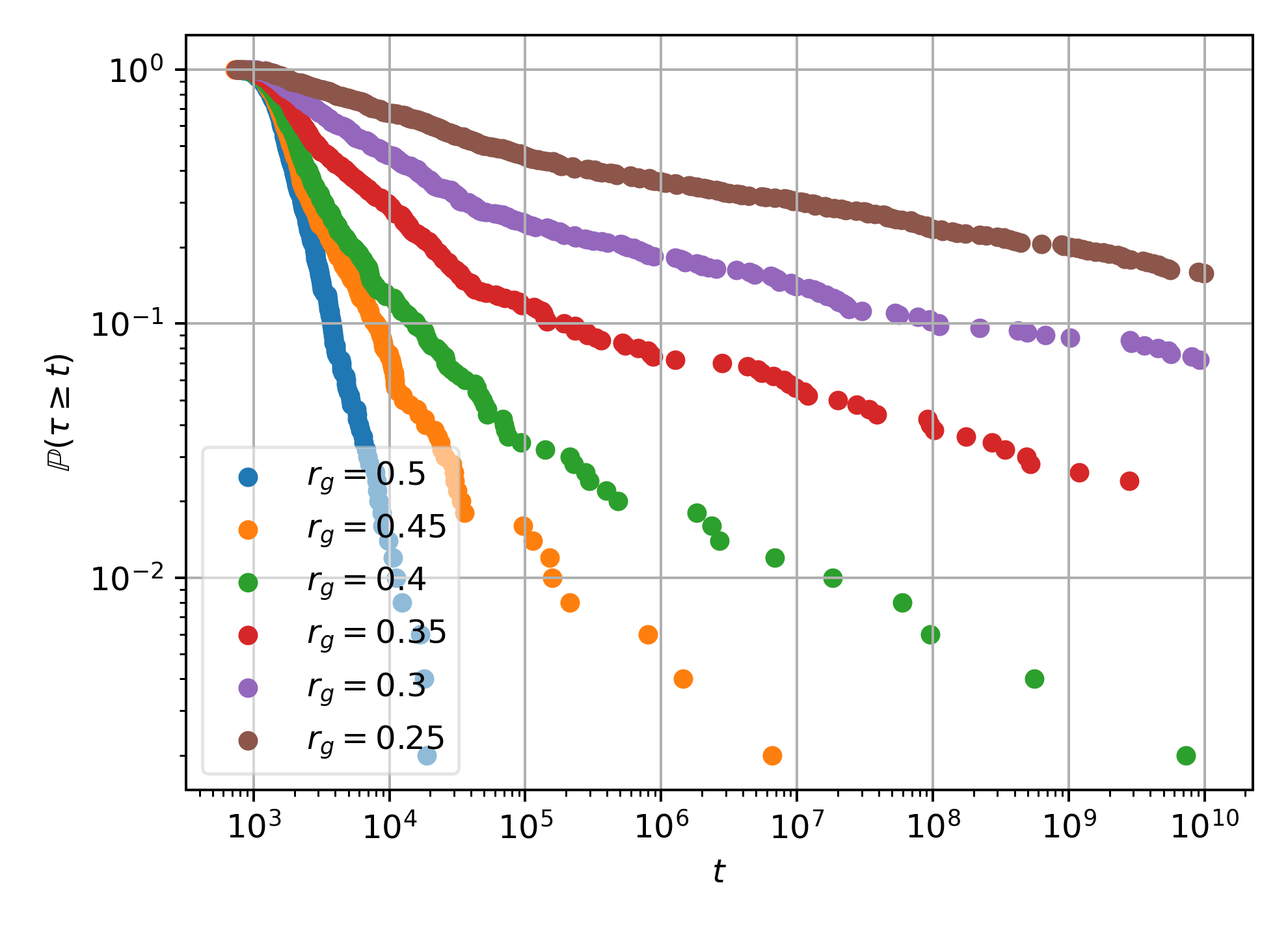
(a) Tail probabilities

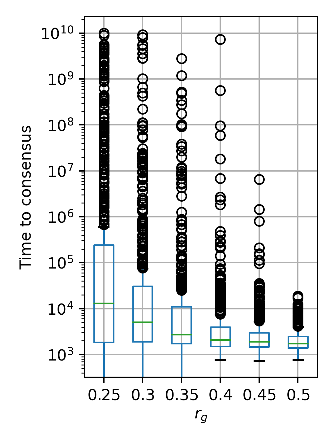
(b) Box and whisker

Figure 2. Tail probabilities ($\mathbb{P}(\tau>t)$) (on a log-log scale) and a box and whisker diagram for the time to consensus for different values of the radius $r_{g}$ used in the random geometric graph model to sample networks. The linear nature of these plots are indicative of a heavy tailed distribution. The high number of outliers on the upper end of the time to consensus is indicative of a heavy-tailed distribution. The parameter settings are detailed in §4.1.

In Figure 2b, we show box and whisker diagrams of the simulated time to consensus (conditioned on $\tau<t_{\text{max}}=10^{10}$). This representation of the simulated data clearly shows that there are many runs which might be identified as ‘outliers.’ This indicates that the time to consensus has a high skewness and like the tail probabilities points toward a heavy-tailed distribution. A possible explanation for the heavy-tails is metastable states, which the system may spend a lot of time in before eventually ‘jumping’ out to consensus. Indeed, similar heavy-tailed survival probabilities were observed for the voter model on small-world networks, which exhibit metastable polarisation [28]. We see that as the radius $r_{g}$ decreases, the probability that consensus is reached after time $t\in\mathbb{R}$ increases. This shows how quantitatively the dynamics do depend on the realisation of the network structure.

To illustrate this phenomenon of metastability, we plot the state of the system at different points in time for a single trajectory. In Figure 3 we show the total number of agents holding opinion $o=1$ over time in this trajectory, which illustrates the metastable behaviour. In Figure 4 we show the network of agents coloured according to their opinion at different time steps. We see that by $t=10^{4}$ two groups emerge; just less than 20 agents holding opinion $o=-1$ and the rest holding opinion $o=1$. This remains the case until shortly after time step $5.82\times 10^{6}$ when the opinions all quickly converge to $o=1.$ The long time spent around one state with many small fluctuations followed by a quick exit to a truly stable state is typical of metastability.

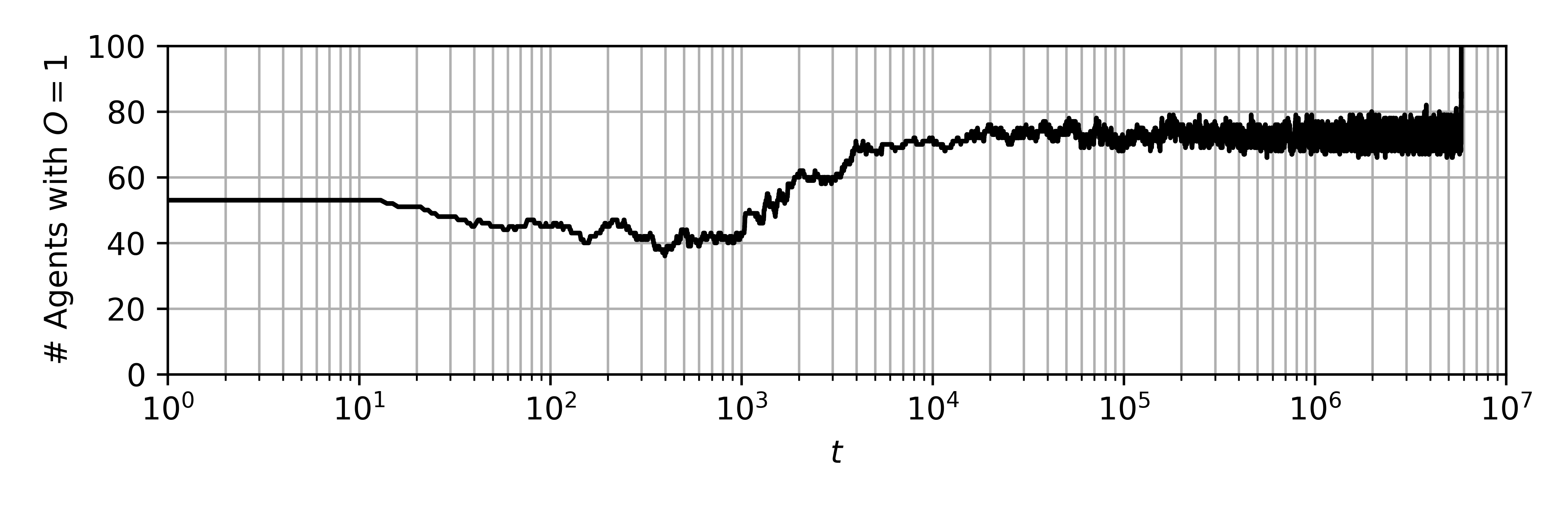
Figure 3. Number of agents holding opinion $o=1$ in a simulation run exhibiting metastable behaviour plotted with time on a logarithmic scale. The state of the network is plotted for telling timestamps of this simulation run in Figure 4. In this simulation run $r_{g}=0.25$, while the rest of the parameters are as described in §4.1.

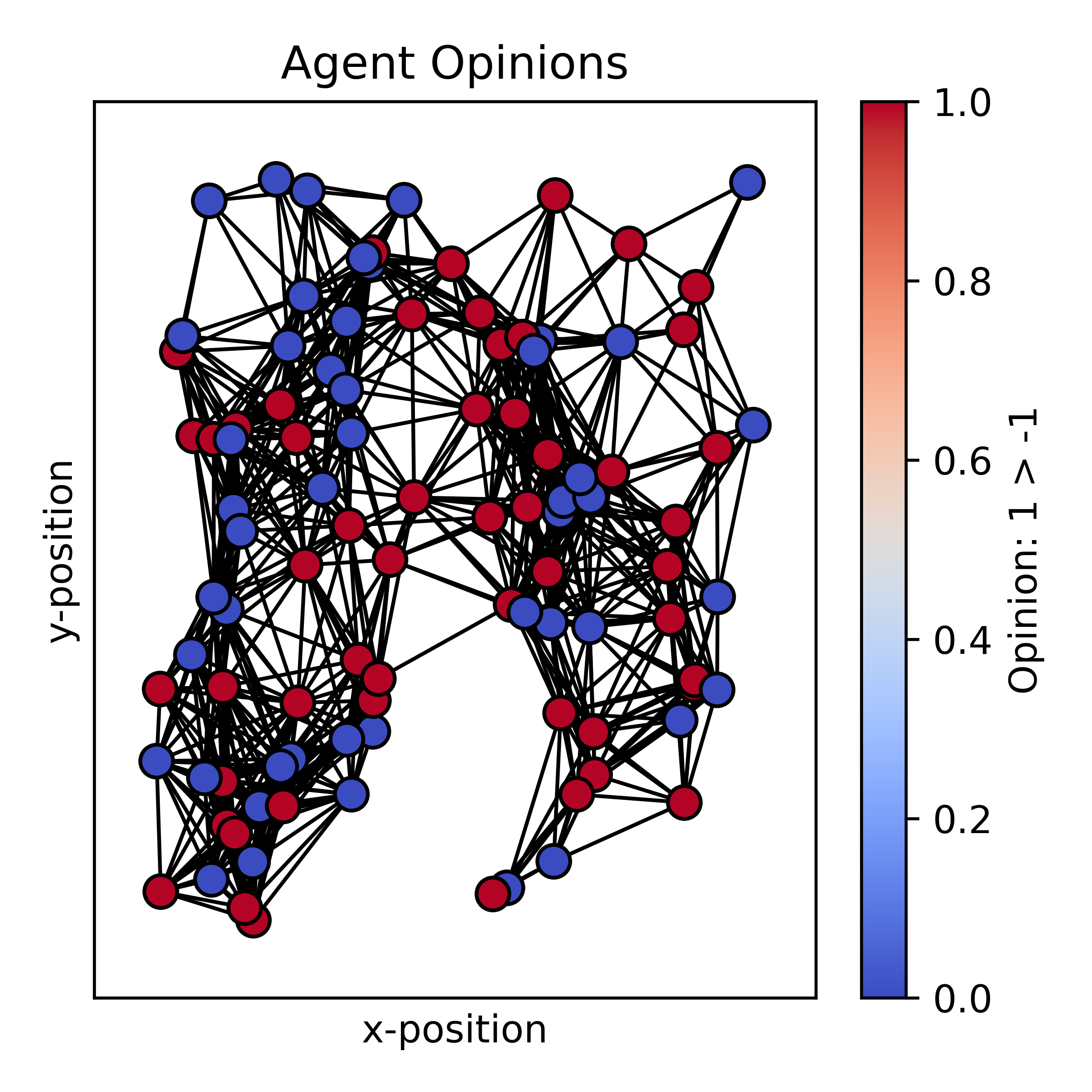
(a) $t=1$

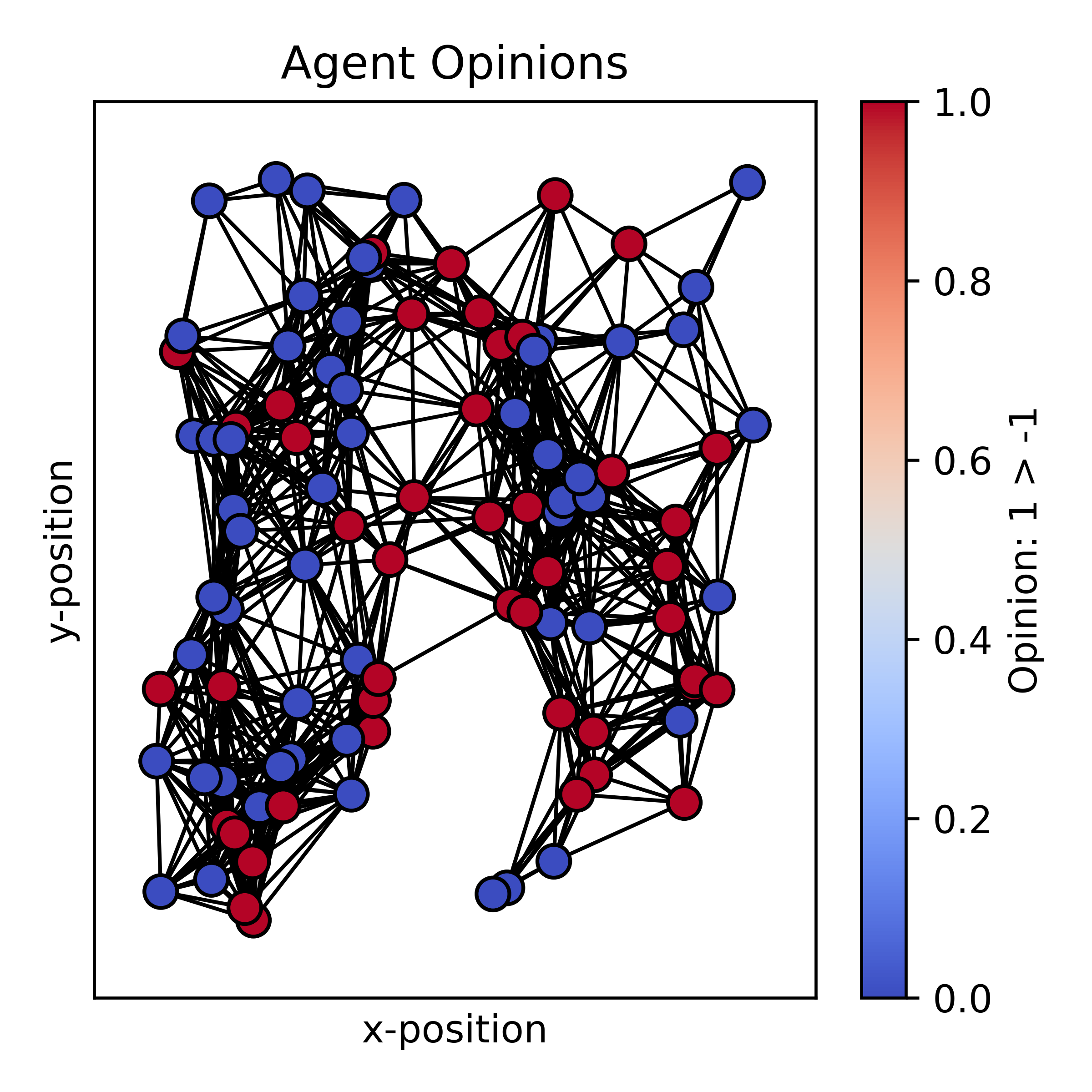
(b) $t=100$

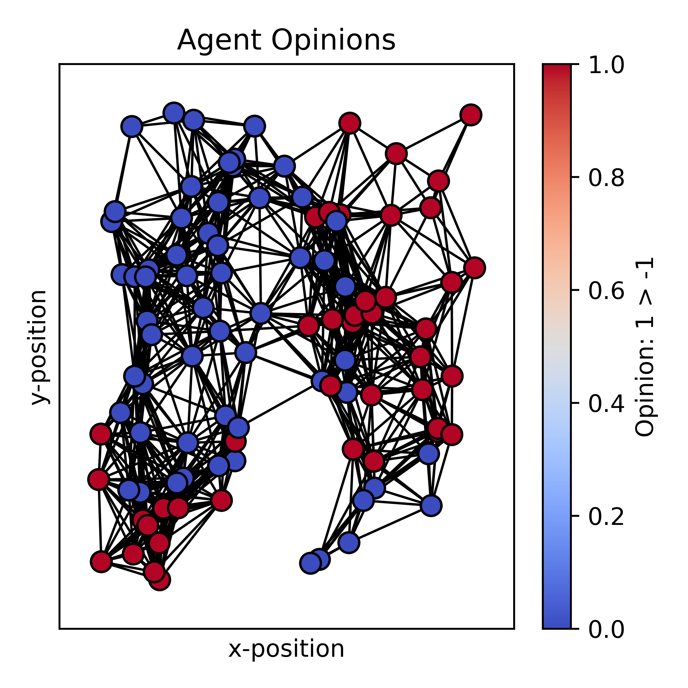
(c) $t=10^{3}$

(d) $t=10^{4}$

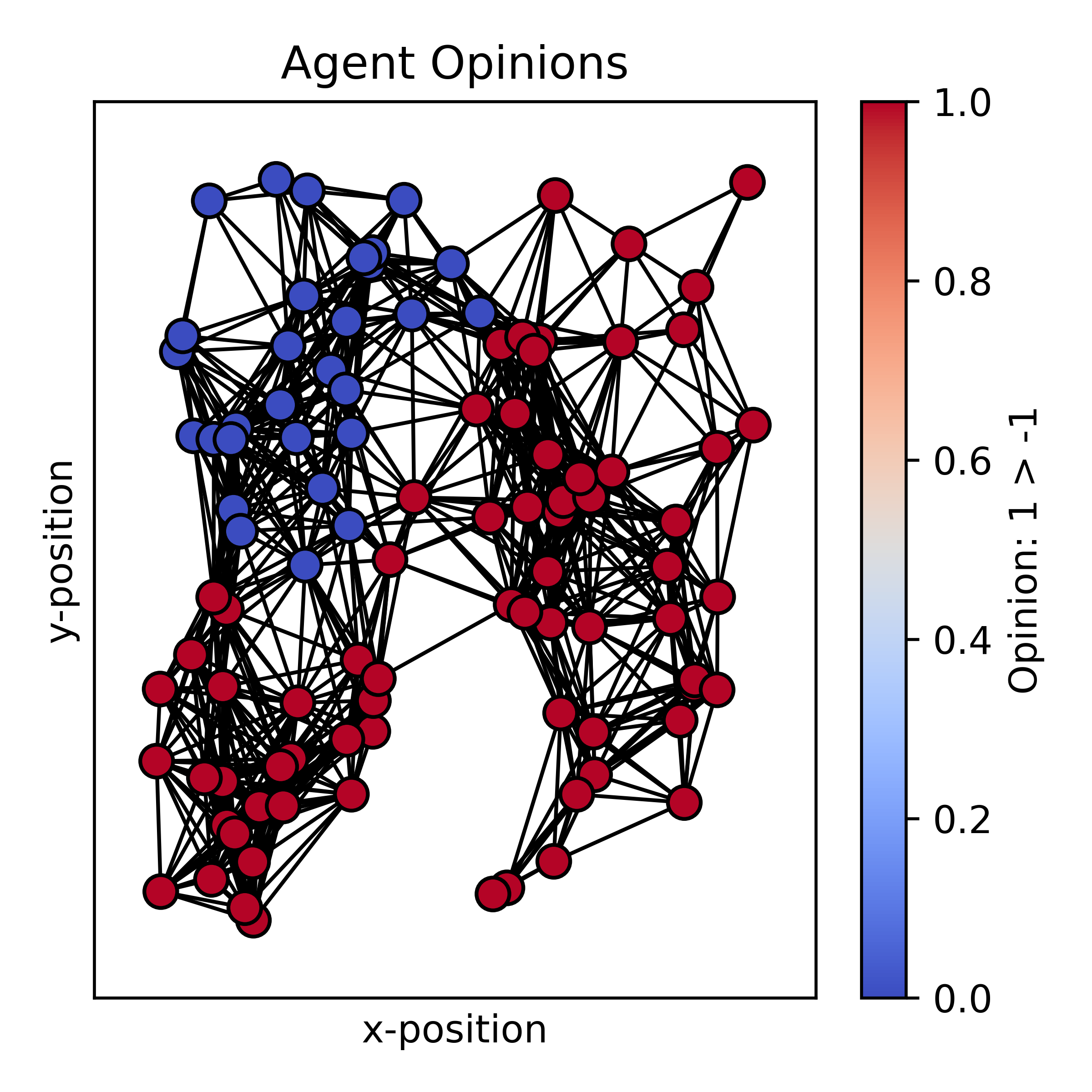
(e) $t=10^{6}$

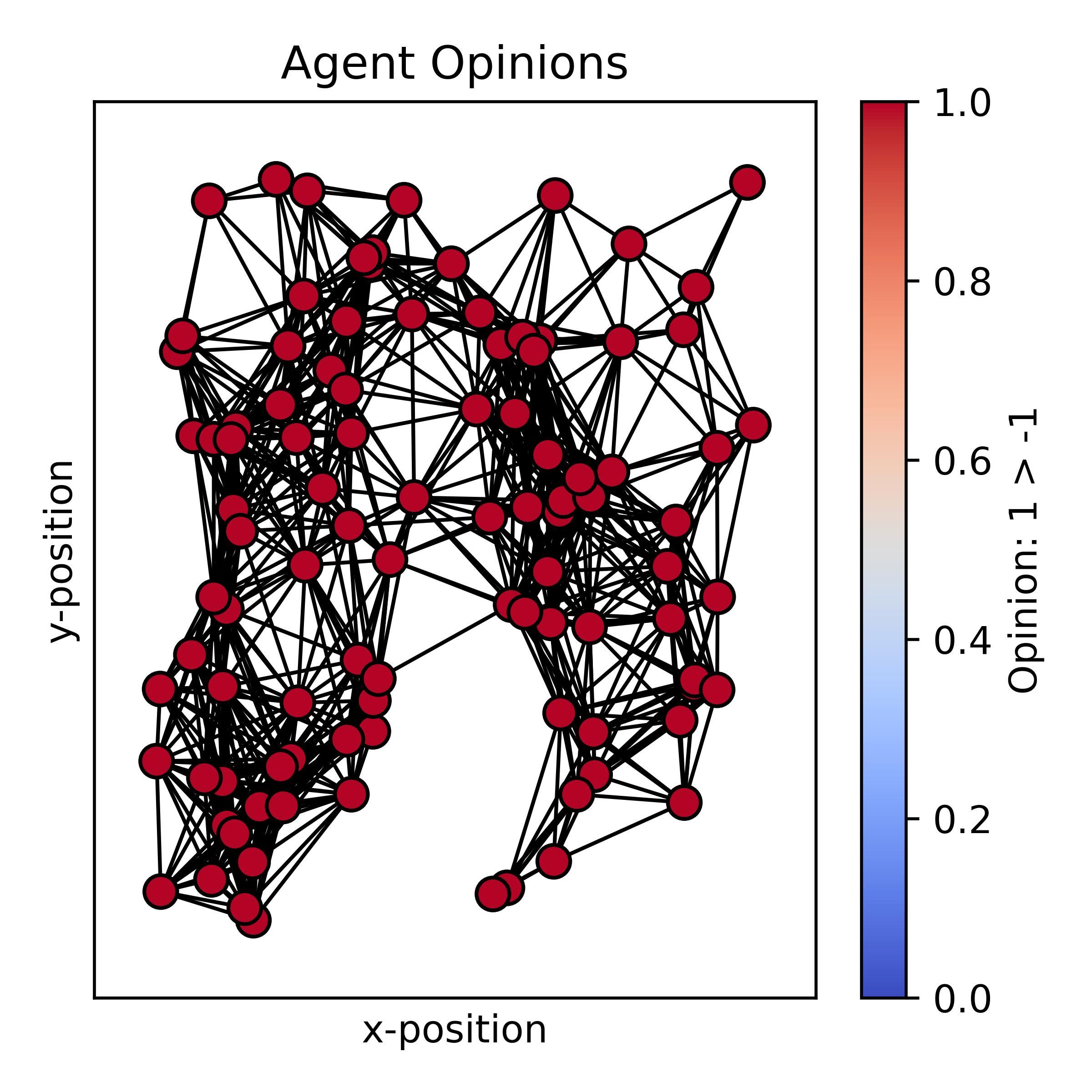
(f) $t\approx 5.82\times 10^{6}$

Figure 4. Opinions in simulation run with metastable behaviour at various timestamps. In particular, note that the group holding opinion $o=-1$ forms around $t=10^{4}$ retains this view until after $t=10^{6}$. Corresponding to this run is the total number of agents holding opinion $o=1$ plotted on a logarithmic timescale in Figure 3. In this simulation run $r_{g}=0.25$, while the rest of the parameters are as described in §4.1.

2.2. Relationship to voter model

It is not clear from the simulations presented by BO or the simulations we have executed that consensus occurs with probability one. Indeed, polarisation may seem stable because many simulation runs ended in a state of polarisation in both sets of numerical simulations. We know that consensus will be reached asymptotically, but how long the process may be in a state of polarisation is not addressed by Theorem 1. To explore the stability of polarisation, we employ a separation of time scales argument which relates the ARLOD model to a different Markov chain, namely, the voter model.

It is well known [33, 34, 35, 36, 37, 38] that reinforcement learning dynamics can be described by the replicator dynamics in the continuous time limit, using a separation of times scales between agent learning and strategy adjustment. We now present a similar relationship between the ARLOD model and the jump chain (discrete time version) of the voter model [25] on a finite topology and in the case of two opinions. It is known that the voter model on scale-free networks [26, 27], and small-world networks [29, 28] exhibits metastable polarisation and truly stable consensus.

To establish the link between Q-learning and the voter model, we define the preference vector at time $t\in\mathbb{N}$: $Y_{t}$ whose elements are:

$$Y_{t}(i)=\begin{cases}1\quad&\text{if }Q_{1}^{i}(t)\geq Q_{-1}^{i}(t),\\ -1&\text{otherwise.}\end{cases}$$ (8)

It takes values in the state space $\mathcal{S}:=\{-1,1\}^{N}$.

Note that we use the weak inequality in (8), though in the limit of interest, equality occurs with probability zero. We define the preference vector for the batched model as $(Y_{t}^{b})_{t\geq 0}$. In essence, the batched model is a biased realisation of ARLOD; in the batch at time $t$ an agent is chosen to express their opinion to a neighbour as often ($b_{t}\in\mathbb{N}$ times) as is needed for them to have the same opinion preference. This occurs in the ARLOD model at probability $(1/N)^{b_{t}}$. For details, see §4.3.

We now state the main result of this section, which relates a batch learning version of the ARLOD model to the discrete time version of the voter model. The details of the voter model and the batch learning version of the reinforcement model are given in §4.2 and §4.3 respectively.

Theorem 2.

For any initial assignment of Q-values resulting in preference vector $Y_{0}=\eta_{0}\in\mathcal{S}$, the random process tracking the change of the preference vector $(Y^{b}_{t})_{t\geq 0}$ in the batch version of the Q-learning model on graph $G$ converges in distribution to the voter model on the same graph:

$$\mathbb{P}(Y^{b}_{t}=\eta)=\mathbb{P}(X_{t}=\eta),\quad\forall\eta\in\mathcal{S},$$ (9)

with $(X_{t})_{t\geq 0}$ Markov($\delta_{\eta_{0}},P$) with $P$ as defined in (14).

The proof is provided in Appendix C and relies on the fact that an agent will receive enough feedback to make the ordering of their Q-values match that of their neighbour in finite time. Thus, we have shown that under a particular separation of time scales, the ARLOD model behaves like the discrete time voter model on a finite graph with two opinions. The construction of the batched ARLOD model and its relation to the voter model ensures that any state that is metastable in the voter model will also be metastable in the ARLOD model.

2.3. Instability of consensus and ergodicity of symmetric reinforcement learning

We now introduce a new model based closely on the ARLOD model, with a subtle difference: both agents involved in an interaction express their opinion in the same way and update their Q-values as a result of what they observe. Because now the roles of the two agents are indistinguishable, we call this the symmetric reinforcement learning for opinion dynamics (SRLOD) model. We show that consensus is no longer absorbing in this model. To differentiate it from the ARLOD model, let $q_{o}^{i}(t)$ denote the Q-value agent $i\in\{1,\ldots,N\}$ has for opinion $o\in\{-1,1\}$ at time $t\in\mathbb{N}$. For the details see §4.4.

Lemma 3 (Consensus is not stable).

If there exists a time $t_{0}\in\mathbb{N}$ such that $q_{o}^{i}(t_{0})>q_{-o}^{i}(t_{0})$ for some opinion $o\in\{-1,1\}$ and each agent $i\in\{1,2,\ldots,N\}$, then

$$\mathbb{P}(q_{o}^{i}(t)>q_{-o}^{i}(t),\forall t\geq t_{0})=0.$$ (10)

The proof of Lemma 3 is presented in Appendix D. This and the next result depend on the fact that any sequence of actions has positive probability in this model because both agents learn from an interaction and explore with probability $\epsilon>0$. In particular, the probability of any finite sequence of actions of length $l<\infty$ occurs with a probability bounded from below by $p(l)$:

$$p(l)=\left(\frac{1}{|E|}\right)^{l}(\epsilon^{2})^{l}>0.$$ (11)

Consensus not being an absorbing state is a fundamental difference between the symmetric and the asymmetric model. To elucidate this difference, we introduce the preference vector, $y_{t}$, of length $N$, whose $i$-th element takes the value:

$$y_{t}(i)=\begin{cases}1\quad&\text{if }q_{1}^{i}(t)\geq q_{-1}^{i}(t)\\ -1&\text{otherwise.}\end{cases}$$ (12)

The preference vector describes which opinion ($1$ or $-1$) each agent $i\in\{1,2,\ldots,N\}$ favours. The dynamics of the preference vector are ergodic in the symmetric model.

Proposition 1 (Time-evolution of the preference vector is ergodic).

The probability of the preference vector transitioning in finite time between any two states $\eta,\zeta\in\mathcal{S}$ is positive, i.e.,

$$\mathbb{P}(y_{t_{0}+k}=\zeta\mid y_{t_{0}}=\eta)>0,\quad\text{for all }\eta,\zeta\in\mathcal{S},\text{and some }k<\infty.$$ (13)

To prove this, one first delineates a finite sequence between any two states $\eta,\zeta\in\mathcal{S}$ and observes that the probability of these sequences is positive by (11). For any two states there is a finite sequence of events which leads from one to the other as all agents take both actions with positive probability, and can always switch their belief in a finite number of rounds. Thus, all states communicate with one another. The ergodicity of the SRLOD model is illustrated in Appendix F.

3. Discussion

We have analysed the ARLOD model of social learning put forth by Banisch and Olbrich [16]. We have shown that consensus is reached asymptotically with probability one for any finite population structure. In particular, this is in contrast with the stability of polarisation originally reported for that model. A small modification of that model, based on symmetrizing the interaction-learning relation between the agents, results instead in ergodic dynamics, which thus destabilizes consensus somewhat. This result mirrors the difference between the voter model and the noisy voter model, in which a random probability of switching one’s opinion is introduced [39, 40].

The highlighted importance of network structure in the original article [16] warrants attention. The theoretical arguments we present here to show that consensus is the only asymptotically stable state in the original model and that the symmetrized model is ergodic required only that the network is connected. Thus, qualitatively, the assumption of network structure is not very important. We do, however, see that it plays a role quantitatively in the time taken for consensus to be reached. Many studies on polarisation and other social dynamics focus on the importance of network structure. It is important to disentangle which outcomes of the model are truly caused by networks structure and which are outcomes based on other — more implicit — modelling decisions.

Having proved that the polarisation observed in the ARLOD model is not asymptotically stable and that consensus is guaranteed, we turn to the original research question. What causes stable polarisation? We provide conditions (a systematic biasing) for which the ARLOD model converges to the voter model. Polarisation can be metastable in the voter model, and, by their relation, also in the reinforcement learning model. This bridges multiagent learning models and models well studied in sociophysics and theoretical biology.

Our results raise questions regarding the possibility of finding a model of opinion dynamics excluding repulsive forces and allowing for stable polarisation. Can we say that a reasonable model of opinion dynamics should exhibit truly stable polarisation? Is the polarisation we observe around us stable or metastable? Future research is required to give an example of such a model or a proof that it does not exist. These questions might be explored by investigating learning in the ‘real world’ (to identify appropriate $\alpha$ and $\epsilon$) as well as the influence of parameter values $\alpha$ and $\epsilon$ in the ARLOD model. It could be that ‘real world’ learning is such that consensus would be reached quickly under the ARLOD model, indicating that a more realistic model requires additional elements. Alternatively, it may be that the parameters of the ‘real world’ are such that the time it takes to exit the metastable polarised state is so long that differentiating between metastable and stable polarisation in the real world is difficult.

4. Methods

4.1. ARLOD simulation settings

We have chosen the parameter settings based on the following considerations. A greater number of agents means that more rounds are required to select each agent sufficiently often to reach consensus. On the other hand, a smaller learning rate increases what ‘sufficiently often’ means per agent, as indicated in (4). To strike a balance between these effects, we set $N=100$ and $\alpha=0.25$. Following BO, we set $\epsilon=0.1$ and initialise the Q-values uniformly in $[-0.5,0.5]$. The radius for the random geometric graph model $r_{g}\in[0.25,0.5]$ is selected to exhibit a range of behaviour, focusing on connected graphs. We have chosen the maximum time to simulate ($10\times 10^{9}$ rounds) and the number of simulation iterations (500 iterations) to be significantly greater than those used by BO ($2\times 10^{6}$ rounds and 100 iterations). This allows the simulation to reach consensus more frequently, which we know occurs eventually with probability one (by Theorem 1).

4.2. Discrete time voter model

In the voter model, nodes on a graph have an opinion, which may take one of two values ${-1,1}$. Repeatedly, a node is selected at random from the set of all nodes. This node performs an update in which it selects one of its neighbours and copies whichever opinion they have. Time may be indexed by each such round, or by a collection of rounds in which on average each node is selected once (on the order of the population size).

We define the discrete time voter model as a Markov chain $(X_{t})_{t\geq 0}$ with $t\in\mathbb{N}$. As such, we define the graph on which the voter model is to take place $G=(V,E)$, with $V$ the set of vertices (voters) and $E$ the set of edges (connections between voters). The number of voters is $|V|=N$ and we endow each vertex $i$ with an opinion $o_{i}\in\{-1,1\}$ for $i\in\{1,\ldots,N\}$. As a result, the state space of the system is all possible assignments of each vertex to an opinion: $\mathcal{S}:=\{-1,1\}^{N}$.

We denote the unit vector of length $N$ with a one at the $l$-th entry and zeros everywhere else as $\bm{e}_{l}$ for $l\in\{1,2,\ldots,N\}$. The transition probability from state $\eta\in\mathcal{S}$ to state $\zeta\in\mathcal{S}$ is denoted $P_{\eta,\zeta}:=\mathbb{P}(X_{t+1}=\zeta\mid X_{t}=\eta)$ and is given by

$$P_{\eta,\zeta}=\begin{cases}0\quad&\text{if }\lVert\eta-\zeta\rVert_{1}>2,\\ \frac{1}{N}\left(\frac{1}{2}-\frac{o_{l}}{2d_{l}}\sum_{k\in N(l)}o_{k}\right)&\text{if }\lVert\eta-\zeta\rVert_{1}=2,\text{and }\zeta=i-2o_{l}\bm{e}_{l},\\ 1-\sum_{\zeta\neq\eta}P_{\eta,\zeta}&\text{if }\zeta=\eta.\end{cases}$$ (14)

Here $d_{l}$ is the degree of voter $l\in V$ and $N(l)$ is their neighbourhood in the graph $G$.

Informally, the transition probability in (14) is simply the uniform probability of agent $i\in\{1,\ldots,N\}$ being chosen, multiplied by the probability of them selecting a neighbour (uniformly at random) holding opinion $-o_{j}$. All transitions from $\eta\in\mathcal{S}$ to $\zeta\in\mathcal{S}$ in which the two states $\eta$ and $\zeta$ differ in more than one position occur with probability zero.

Given a starting assignment of opinions to voters $\eta\in\mathcal{S}$, the voter model is the Markov process $(X_{t})_{t\geq 0}$ that is Markov($\delta_{\eta},P$), taking values in $\mathcal{S}$. Here $\delta_{\eta}$ is the delta function. Alternatively, given a distribution of the possible starting assignments of opinions to voters $\lambda$ such that $\mathbb{P}(X_{0}=\eta)=\lambda_{\eta}$ for each $\eta\in\mathcal{S}$, the voter model is Markov($\lambda,P$).

The dynamics of the voter model are illustrated in Figure 5. In this example, we consider $5$ voters, $V=\{1,\ldots,5\}$ with connections $E=\{(1,2),(1,3),(1,4),(2,3),(2,5),(3,5),(4,5)\}$ and initial opinions $X_{0}=[-1,1,1,-1,1]$. We show the transitions conditioned on voter $1$ being selected to copy the opinion of one of their neighbours. In particular, if voter $1$ selects voters $2$ or $3$ they switch their opinion and if they select voter $4$ they keep their current opinion. These transitions occur with probability $2/3$ and $1/3$, respectively.

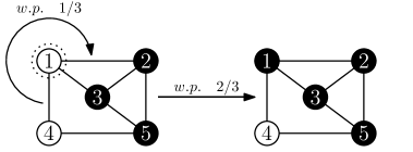
Figure 5. Illustration of the voter model dynamics. We show the transition probabilities conditioned on voter $1$ being selected to copy the opinion of one of their neighbours at random.

4.3. Asymmetric Q-learning in batches

The concept of multi-agent learning in batches has been explored in its own right [41, 42, 43]. It may be interpreted as a separation of time scales. That is, the rate at which agents learn about the behaviour of the environment or the other agents is faster than the rate at which they adjust their behaviour. Practically, it may be implemented by defining a batch size $b\in\mathbb{N}$ which constitutes a number of rounds in which the agent keeps their behaviour fixed and collects samples from their environment. At the end of this batch, the belief of the agent is updated using all the observations made during the batch.

Now we define the batch learning version of the ARLOD model. In particular, agent $i$ chosen to express their opinion in batch $t\in\mathbb{N}$ will express their opinion to their chosen neighbour $j$ in a batch of size $b_{t}\in\mathbb{N}$.

That is, the dynamics follow the steps:

1. At time $t$, an agent $i\in\{1,2,\ldots,N\}$ is selected uniformly at random from the population.

2. This agent $i$ chooses a neighbour $j$ from their neighbourhood $N(i)$ uniformly at random.

3. Then follow a sequence of subrounds indexed $s=1,\ldots,b_{t}$. Because agent $i$ is the only agent who can adjust their belief in this batch, we denote agent $i$’s Q-values in the subround $s$ by $Q^{\prime}(s)$ and their opinion preference $Y_{s}^{\prime}$ (with $Q^{\prime}(0)=Q^{i}(t)$ and $Y_{0}^{\prime}=Y^{b}_{t}(i)$). In each subround, agent $i$ expresses an opinion to agent $j$, following the rules of the ARLOD model:

   • expressing their preferred opinion $o_{i}(s)=Y_{s}^{\prime}$ at probability $1-\epsilon$,

   • expressing their disfavoured opinion $o_{i}(s)=-Y_{s}^{\prime}$ at probability $\epsilon$, and

   • incorporating agent $j$’s honest response $R_{j}(s)$ into their $Q^{\prime}$ value $Q_{o_{s}}^{\prime}.$

   Now we define the random batch size $b_{t}=\min\{s:Y_{s}^{\prime}=Y_{t}(j)\}$, i.e., the number of subrounds required until agent $i$’s preference matches that of agent $j$.

4. Agent $i$ updates their Q-values: $Q^{i}(t+1)\leftarrow Q^{\prime}(t+b_{t})$.

We use this perhaps unconventional construction because the techniques in [44] are not applicable here, as the states are not lumpable.

On a high level, the procedure of one such time step is depicted in Figure 6.

Figure 6. The dynamics in one time step of the batched version of the ARLOD model at a high level of abstraction. Agent $i$ expresses an opinion $b_{t}$ times to their neighbour agent $j$ who responds each time. Thereafter, agent $i$ updates their Q-values with all the feedback they received.

4.4. Symmetric reinforcement learning

A population of $n\in\mathbb{N}$ agents is embedded in a random (connected) geometric network topology. In each discrete time step $t\in\mathbb{N}_{\geq 0}$ an edge $(i,j)\in E$ is selected uniformly at random. The two agents on either end of this edge $i$ and $j$ express an opinion to one another $o_{i}(t),o_{j}(t)\in\{-1,1\}$. Subsequently, both agents update the Q-value of their expressed opinion as follows:

$$q_{o_{i}(t)}^{i}(t+1) =q_{o_{i}(t)}^{i}(t)(1-\alpha)+\alpha o_{i}(t)o_{j}(t)$$ (15)

$$q_{o_{j}(t)}^{j}(t+1) =q_{o_{j}(t)}^{j}(t)(1-\alpha)+\alpha o_{i}(t)o_{j}(t),$$ (16)

where $\alpha\in(0,1)$ is the learning rate. The Q-value of the opinion the agents did not express is not updated. We call the opinion $o$ such that $q_{o}^{i}(t)>q_{-o}^{i}(t)$ agent $i$’s preferred opinion. We assume that both agents express their preferred opinion with probability $1-\epsilon$ (called exploitation) and express their disfavoured opinion with probability $\epsilon$ (called exploration).

The difference thus between this model and the original model is only that instead of a one-sided interaction, both agents may explore and learn from the interaction each round.

4.5. Random connected geometric graphs

The algorithm to generate a connected random graph is provided in Appendix E. We use the subroutine for the generation of a random geometric network from the Python NetworkX package [45]. For a detailed discussion on random geometric graphs and their properties, the interested reader is referred to [31, 46]. The random geometric graph model is popular in the context of social dynamics because it mimics the homophily of real social networks [47].

The general idea of the random geometric graph is to distribute the desired number of nodes randomly in Euclidean space (we use $[0,1]^{2}$) and fixes a radius $r_{g}$. Subsequently, any nodes $u,v$ that are distance $d(u,v)<r_{g}$ from one another are connected by an edge $(u,v)$. Because we are interested in connected networks, we simply repeat the standard procedure until a connected graph is sampled. We take care to only use $r_{g}$ for which the probability of sampling a connected graph is sufficiently high (as described in §4.1).

Appendix A Proof of Lemma 1

Proof.

We proceed by induction on time. Suppose that $Q_{o}^{i}(t_{0})>Q_{-o}^{i}(t_{0})$ at time $t_{0}\geq 0$, for some opinion $o\in\{-1,1\}$, and each agent $i\in\{1,2,\ldots,N\}$.

The base case is that in round $t_{0}+1$, the ordering of all the Q-values will remain the same.

In round $t_{0}$, any agent $i\in\{1,2,\ldots,N\}$ may be chosen to express their opinion to one of their neighbours.

Case 1. Suppose they exploit their preferred opinion (the one with greater Q-value). Any agent they express their opinion to, has the same ordering among their Q-values by the conditions of the lemma, and so responds with an action that leads to a positive reward. Thus,

$$Q_{o}^{i}(t_{0}+1)\geq Q_{o}^{i}(t_{0}),$$ (17)

the Q-value of the preferred opinion in round $t_{0}+1$ is at least as great as in $t_{0}.$

Case 2. Suppose they explore by taking the action with lesser Q-value. Any neighbour they express this opinion to responds honestly. By the assumption, all agents have the same Q-value ordering, so the honest response to exploration is an action that leads to a punishment. Thus,

$$Q_{-1}^{i}(t_{0}+1)\leq Q_{-1}^{i}(t_{0}),$$ (18)

the Q-value of the disfavoured action in round $t_{0}+1$ is lower than or equal to what it was in round $t_{0}$. This is true because the Q-values are initialised to be in $[-1,1]$ and will stay therein indefinitely by the updating prescribed.

This proves the base case (as this holds for all agents that could have been chosen in round $t_{0}$): $Q_{o}^{i}(t_{0}+1)>Q_{-o}^{i}(t_{0}+1)$ for all agents $i\in\{1,2,\ldots,N\}$.

In the induction step we assume it is true until rounds $t_{0}+n$ for $n>0.$ To show that it is true for all rounds up until $t_{0}+n+1$, we simply follow the same procedure as in the base case but for the game in round $t_{0}+n$ which determines the Q-values in round $t_{0}+n+1$. ∎

Appendix B Proof of Lemma 2

Proof.

First, we delineate a sequence of events of finite length which may lead from any state to consensus. Secondly, we will show that this sequence of events has positive probability.

Suppose agent $i$ favours opinion $o$ and has a neighbour $j$ who prefers opinion $-o$, all at time $t_{0}$. If agent $i$ is drawn to express their opinion to agent $j$ every round for $L\in\mathbb{N}$ rounds and always exploits their preferred opinion, the Q-value for this opinion is given by:

$$Q_{o}^{i}(t_{0}+l)=Q_{o}^{i}(t_{0}+l-1)(1-\alpha)-\alpha,$$ (19)

for all $l=1,2,\ldots,L$. A term by term comparison shows that this is bounded from above by

$$Q_{o}^{i}(t_{0}+l)\leq Q_{o}^{i}(t_{0}+l-1)(1-\alpha),$$ (20)

since $\alpha\in(0,1)$. Thus, an upper bound of the Q-value in round $t_{0}+l$ is given by $Q_{o}^{i}(t_{0})(1-\alpha)^{l}$ for all $l=1,2,\ldots,L$ as long as $Q_{o}^{i}(t_{0})>0$.

Subsequently, if agent $i$ is drawn to express their opinion to agent $j$ another $M\in\mathbb{N}$ times and explores their disfavoured action in each of these rounds, this opinion’s Q-value follows:

$$Q_{-o}^{i}(t_{0}+L+m)=Q_{-o}^{i}(t_{0}+L+m-1)(1-\alpha)+\alpha,$$ (21)

for all $m=1,2,\ldots,M$. A term by term comparison shows that this is bounded from below by

$$Q_{-o}^{i}(t_{0}+L+m)\geq Q_{-o}^{i}(t_{0}+L+m-1)(1-\alpha).$$ (22)

Again a lower bound to this Q-value in round $t+0+L+m$ is given by $Q_{-o}^{i}(t_{0}+L)(1-\alpha)^{m}$ as long as $Q_{-o}^{i}(t_{0}+L)<0$.

We bound from above the number of rounds needed for any agent’s opinion to be switched, by the number of rounds needed should they start as far away from one another as possible, $\bm{Q}=(-1,1),$ or $(1,-1)$ and be set to cross at zero. The Q-value of the originally preferred opinion reaches $\xi\in(0,\alpha)$ at least by the lowest integer $r$ which satisfies:

$$Q_{o}^{i}(t_{0})(1-\alpha)^{r}\leq\epsilon,$$ (23)

if they express this preferred opinion in each round. Dividing by $Q_{o}^{i}(t_{0})$, taking the logarithm on both sides and rearranging we get

$$r=\bigg{\lceil}\frac{\log(\xi/Q_{o}^{i}(t_{0}))}{\log(1-\alpha)}\bigg{\rceil}.$$ (24)

By a similar procedure we see that the Q-value of the originally disfavoured opinion reaches $-\epsilon$ after a further $r$ interactions (of exploring in each subsequent round). After two more interactions in which the agent expresses each opinion once, the Q-value ordering has switched:

$$Q_{-o}^{i}(t_{0}+2r+2)\geq-\xi(1-\alpha)+\alpha>\xi(1-\alpha)-\alpha\geq Q_{o}^{i}(t_{0}+2r+2),$$ (25)

as long as $\alpha>\xi$, which is satisfied by an appropriate choice of $\xi$.

The number of rounds this takes is $2r+2$. The probability that this happens is bounded by the probability of the agent $j$ being drawn to express their opinion to agent $k$ $2r+2$ times, multiplied by the probability that they take the required action in each round. This is a lower bound because it does not matter whether agent $i$ first exploits $r+1$ times and then explores $r+1$ times in that order. It only matters that there is a total of $r+1$ explorations and exploitations in the $2r+2$ rounds. Thus, the probability $p_{\text{switch}}$ of one agent switching their opinion (if they have at least one neighbour that disagrees with them) is lower bounded by

$$p_{\text{switch}}>(1-\epsilon)^{r+1}\epsilon^{r+1}\left(\frac{1}{N(N-1)}\right)^{2r+2}>0.$$ (26)

Here, agent $i$ is drawn to express their opinion with probability $1/N$ and we bound the probability that they express this opinion to agent $k$ from below by $1/(N-1)$ as that is the maximum possible degree for any agent in the network. This probability is greater than zero simply because it is a finite product of positive numbers.

In a connected population of $N$ agents which is not yet in consensus, there is always at least one edge which has an agent who prefers opinion $o$ on one side and opinion $-o$ on the other side. Furthermore, in the initial state there are at most $N-1$ agents who prefer the ‘wrong’ opinion at time $t_{0}$. So with probability $p>p_{\text{switch}}^{N-1}>0$, in $(N-1)(2r+2)<\infty$ rounds all $N$ agents hold the same opinion. ∎

Appendix C Proof of Theorem 2, Alternative batch definition

Proof.

At time $t=0$, by definition, we have that $\mathbb{P}(Y_{0}=\eta_{0})=1$ which is also true for $X_{t}$ under $\delta_{\eta_{0}}$: $\mathbb{P}(X_{0}=\eta_{0})=1.$

Next we show that for $t\in\mathbb{N}$,

$$\mathbb{P}(Y_{t+1}=\eta\mid Y_{t}=\eta_{t},\ldots,Y_{0}=\eta_{0})=\mathbb{P}(Y_{t+1}=\eta\mid Y_{t}=\eta_{t})=P_{\eta_{t},\eta}.$$ (27)

The $Y_{t+1}$’s independence on $Y_{t-1},\ldots,Y_{0}$ follows from the fact that in the batch at time $t\in\mathbb{N}$ the agents determine their behaviour entirely from the state $Y_{t}$. Expressing agents express their favoured opinion with probability $1-\epsilon$ and express their disfavoured opinion with probability $\epsilon.$ Responding agents always do so honestly, rewarding their favoured opinion and punishing their disfavoured opinion.

Note that $\mathbb{P}(Y_{t+1}=\eta\mid Y_{t}=\eta_{t})=0$ whenever $\lVert\eta-\eta_{t}\rVert_{1}>2$, just as in (14). This is because as soon as $\lVert\eta-\eta_{t}\rVert_{1}>2$ we have that more than one agent has switched their opinion after the batch at time $t$. This is impossible because only one agent updates their Q-values during a batch.

We proceed in two cases, one when $\lVert\eta-\eta_{t}\rVert_{1}=2$ and the other when $\lVert\eta-\eta_{t}\rVert_{1}=0$. Note that $\lVert\eta-\eta_{t}\rVert_{1}\neq 1$ because $\eta,\eta_{t}\in\mathcal{S}=\{-1,1\}^{N}$.

Case 1. $\lVert\eta-\eta_{t}\rVert_{1}=2$: In this case states $\eta$ and $\eta_{t}$ differ in exactly one position which, without loss of generality, we label $l$. In order for agent $l$ to switch their favoured opinion in batch $t$, they must be selected uniformly at random to express their opinion to one of their neighbours. This happens at probability $1/N$.

If an agent expresses their opinion to an agent who favours opinion $-o_{l}$, agent $l$, gets punished for each time they express their favoured opinion and rewarded for each time they express their disfavoured opinion. Thus, if agent $l$ expresses their favoured opinion at least $r+1$ times and their disfavoured opinion at least $r+1$ times, where

$$r=\bigg{\lceil}\frac{\log(\epsilon)}{\log(1-\alpha)}\bigg{\rceil},$$ (28)

then their opinion will have switched (see the proof of Lemma 2). Thus, we can lower bound the probability of the agent switching their opinion after $2r+2$ rounds by

$$p_{\text{switch}}\geq\epsilon^{r+1}(1-\epsilon)^{r+1}.$$ (29)

Then the probability that the agent does not switch their opinion in finite time is upper bounded by $\lim_{k\to\infty}(1-p_{\text{switch}})^{k}=0$. This means that if the agent has selected to express their opinion to an agent who favours opinion $-o_{l}$, they will switch their opinion, and this will happen in finite time.

The probability of agent $l$ switching their opinion is given by the probability that they select a neighbour favouring the opposite opinion to theirs. As before, we denote $d_{l}$ as the degree of agent $l$. Furthermore, we denote with $a(l)$ and $c(l)$ the number of agents in $l$’s neighbourhood who are in agreement and contradiction with $l$ respectively. Then, because agents select a neighbour uniformly at random, the probability of $l$ switching their opinion is

$$\mathbb{P}(o_{l}\to-o_{l})=\frac{c(l)}{d_{l}}.$$ (30)

This may be rewritten and rearranged as follows:

$$\mathbb{P}(o_{l}\to-o_{l}) =\frac{c(l)}{2d_{l}}+\frac{c(l)}{2d_{l}}$$ (31)

$$=\frac{c(l)}{2d_{l}}+\frac{d_{l}-a(l)}{2d_{l}}$$ (32)

$$=\frac{1}{2}\left(1+\frac{c(l)-a(l)}{d_{l}}\right).$$ (33)

To extract this from $Y_{t}$, notice that it can be rewritten as

$$\mathbb{P}(o_{l}\to-o_{l})=\frac{1}{2}\left(1-\frac{Y_{t}(l)}{d_{l}}\sum_{k\in N(l)}Y_{t}(k)\right),$$ (34)

where $N(l)$ is the neighbourhood of agent $l$ in the graph $G$. Multiplying this by $1/N$, the probability that agent $l$ is selected to express their opinion in the first place, we get precisely $P_{\eta_{t},\eta}$ as required.

Case 2. $\lVert\eta-\eta_{t}\rVert_{1}=0$: In this case, an agent is selected to express their opinion, and they do so to a neighbour who is in agreement with them (in which case $b_{t}=1$). Given that agent $l$ is selected, this happens with probability

$$\mathbb{P}(o_{l}\to o_{l})=1-\frac{1}{2}\left(1-\frac{Y_{t}(l)}{d_{l}}\sum_{k\in N(l)}Y_{t}(k)\right).$$ (35)

This is exactly $1-NP_{\eta_{t},\eta}$ for $\eta=\eta_{t}-2Y_{t}(l)\bm{e_{l}}$. Summing over all agents that might be selected and multiplying by the probability of selecting those agents, we get the required probability of transitioning to the same state, $P_{\eta_{t},\eta_{t}}=1-\sum_{\eta\neq\eta_{t}}P_{\eta_{t},\eta}$. ∎

Appendix D Proof of Lemma 3

Proof.

We show that a sequence of events which leads from consensus to not-consensus is of finite length and positive probability.

Observe that each agent explores (expresses and reinforces the disfavoured opinion) at probability $\epsilon>0$. Observe also that if this disfavoured opinion is reinforced maximally $\kappa+1$ times with

$$\kappa=\bigg{\lceil}\frac{\log(\epsilon)}{\log(1-\alpha)}\bigg{\rceil},$$ (36)

which is finite, and similarly if their preferred opinion is punished $\kappa+1$ times, that they switch ordering of opinion Q-values .

Given a sequence of agent actions, the probability that they take the action in some round required by the sequence, is always bounded from below by $\epsilon>0$. This is because they express their disfavoured opinion at probability $\epsilon$ and their favoured opinion at probability $1-\epsilon>\epsilon$.

This means that the probability of any finite sequence of actions of length $l<\infty$ occurs at a probability bounded from below by $p(l)$ defined in (11). Thus, the probability of an agent exploring and being rewarded $\kappa+1$ times and exploiting and being punished $\kappa+1$ times is positive because this is a sequence of events with length $2\kappa+2$. This is the maximal length sequence which leads to one agent changing the ordering of their Q-values. So we have that the probability that such a switch never happens (the probability of consensus for all $t\geq t_{0}$):

$$\mathbb{P}(q_{o}^{i}(t)>q_{-o}^{i}(t),\forall t\geq t_{0})\leq\lim_{k\to\infty}(1-p(2\kappa+2))^{k}=0.$$ (37)

Therefore consensus is not absorbing (and not a stable state). ∎

Appendix E Algorithm to generate a geometric random graph

1

Input : $N$: number of nodes, $r_{g}$: radius

Output : $G$: connected random geometric graph

2

3$Check\leftarrow$ True;

4 while $Check$ do

5       $G\leftarrow$ empty graph;

6       for $i\leftarrow 1$ to $N$ do

7             Add node $i$ with random coordinates in $[0,1]^{2}$ to $G$;

8            

9       end for

10      for each pair of nodes $(u,v)$ in $G$ do

11             if distance($u$, $v$) $\leq r_{g}$ then

12                   Add edge $(u,v)$ to $G$;

13                  

14             end if

15            

16       end for

17      if $G$ is connected then

18             $Check\leftarrow$ False

19       end if

20      

21 end while

Algorithm 1 Generate Random Geometric Graph with $N$ nodes and radius $r_{g}.$

Appendix F Illustration of the ergodicity in the SRLOD model

The dynamics of the SRLOD model are ergodic by Proposition 1, meaning that the process can reach all states from all other states. In the ergodic setting on a finite state space, one can look for a stationary distribution. That is a probability distribution over the states reporting the probability of observing each state as $t\to\infty$. Thus, the questions one might ask of the model changes from ‘What is the probability of consensus?’ to ‘What proportion of time does the system spend in each state?’ To illustrate the ergodicity of the SRLOD model, we show a simulation run in which consensus was reached on both opinions in Figures 7 and 8.

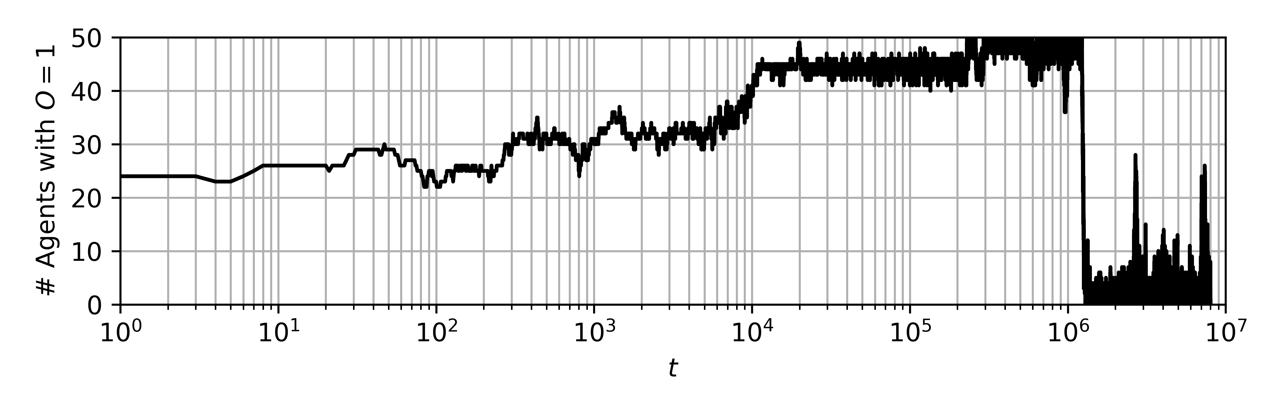
Figure 7. The number of agents holding opinion $o=1$ in a simulation run of the SRLOD model plotted with time on a logarithmic scale. Notice the switch from consensus on opinion $o=1$ to opinion $o=-1$ shortly after $t=10^{6}$.

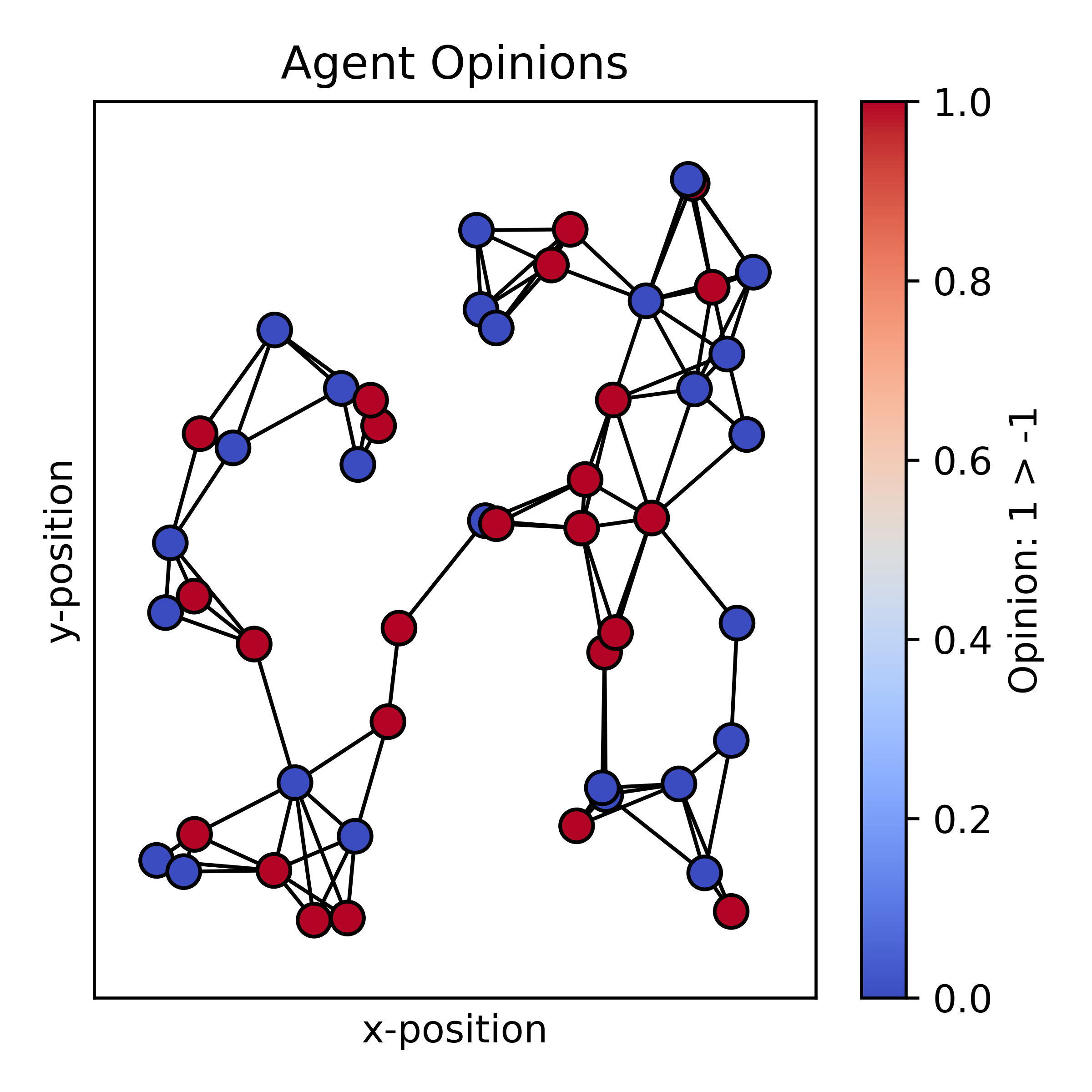
(a) $t=1$

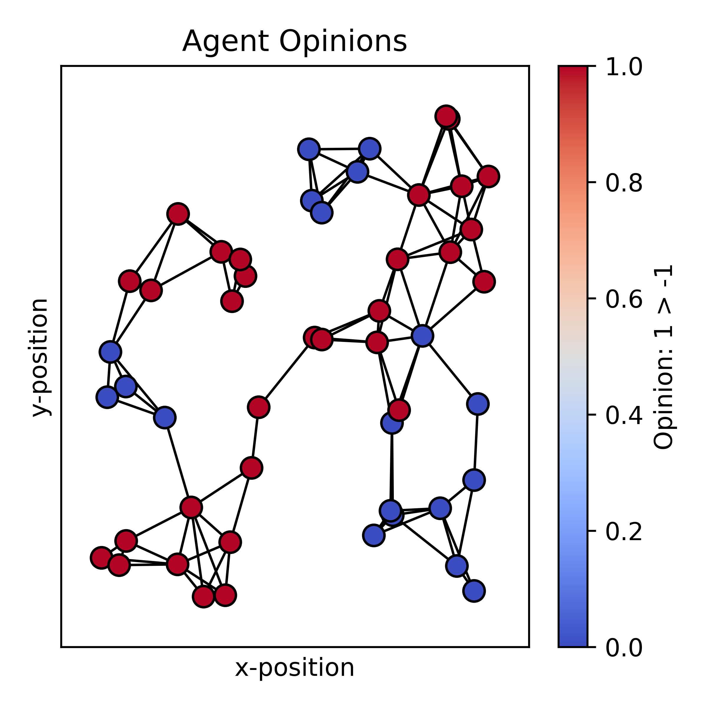
(b) $t=100$

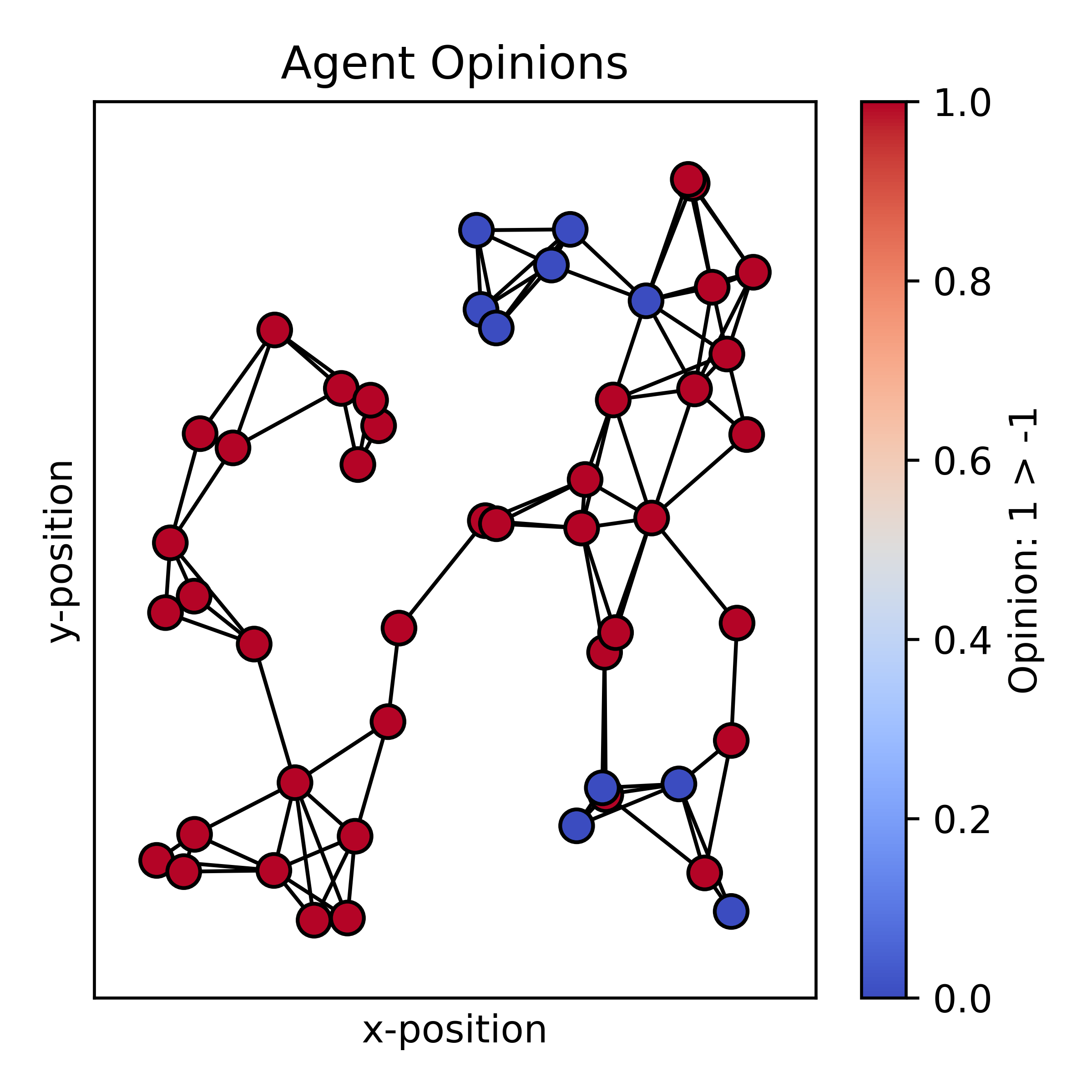
(c) $t=10^{3}$

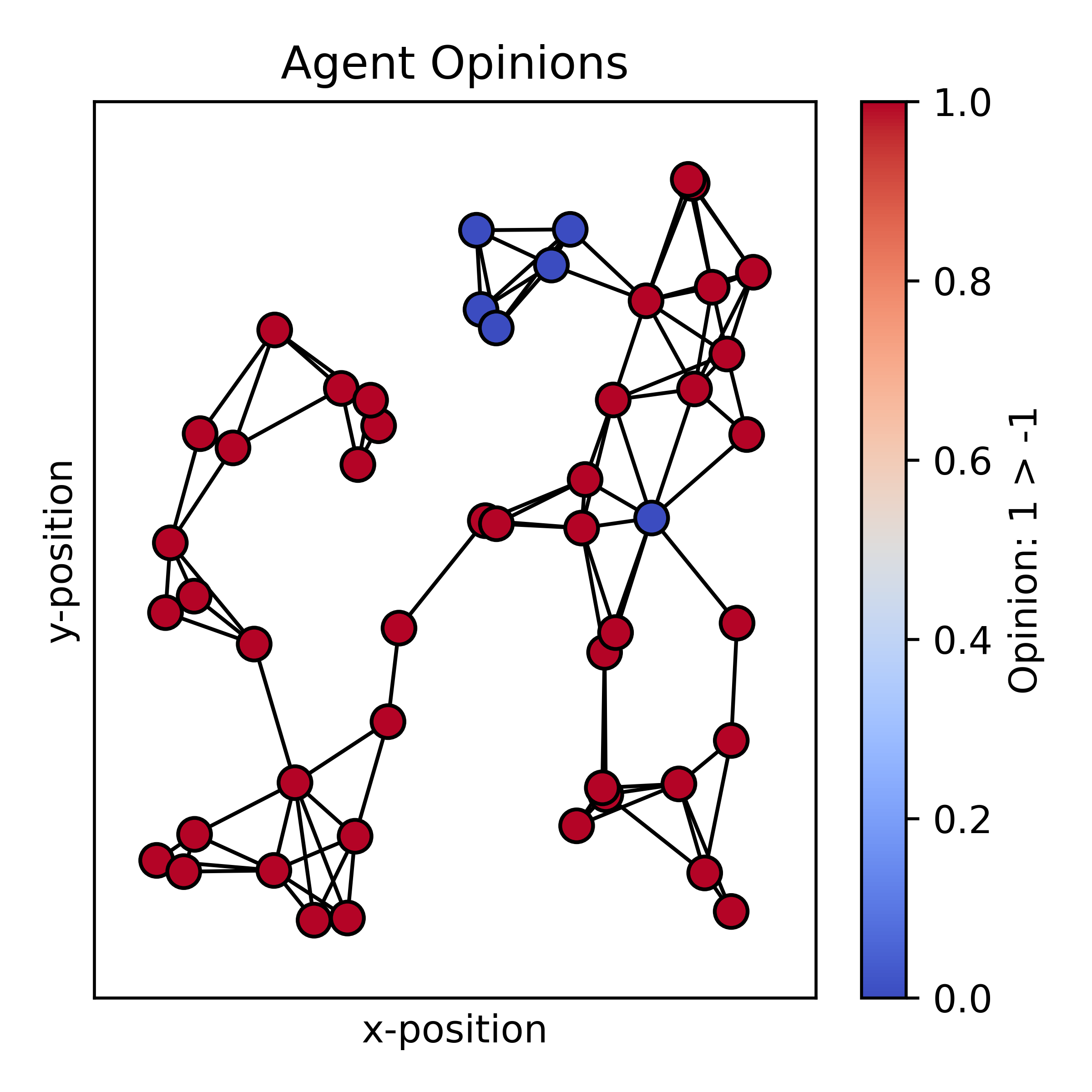
(d) $t=2\times 10^{5}$

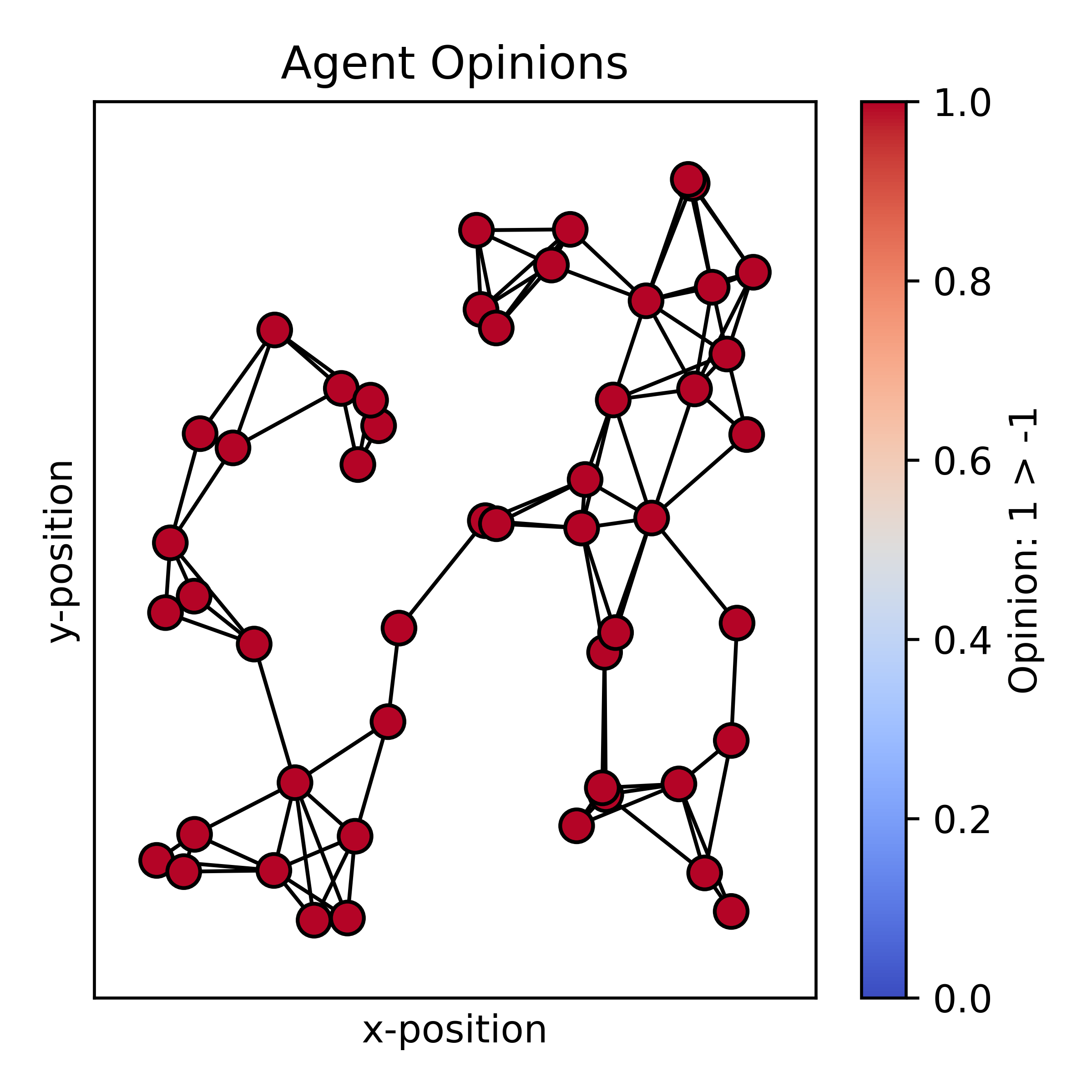
(e) $t=3\times 10^{5}$

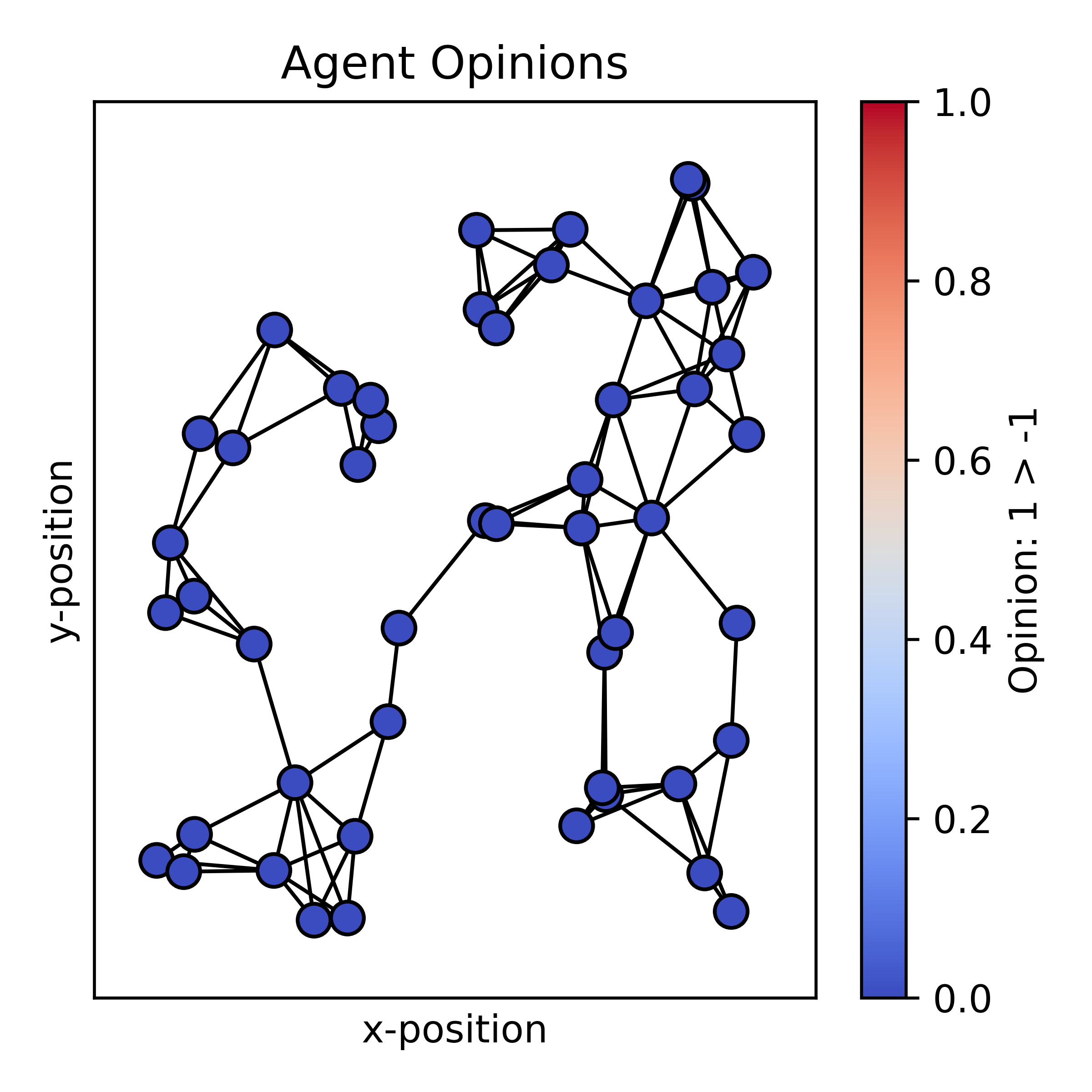
(f) $t=2\times 10^{6}$

Figure 8. Opinions in simulation run of the SRLOD model at specific rounds. Notice the switch from consensus on opinion $o=1$ to opinion $o=-1$ between $t=3\times 10^{5}$ and $t=2\times 10^{6}$.

In this simulation we set $\alpha=0.25$, $\epsilon=0.2$, $N=50$ and $r_{g}=0.2$. Because consensus is no longer absorbing, we stop the simulation manually at $t=8\times 10^{6}$. The number of agents holding opinion $o=1$ is plotted on a logarithmic timescale in Figure 7 while the state of the network is shown for telling rounds in Figure 8.

References

- [1] R. P. Abelson, “Mathematical models of the distribution of attitudes under controversy,” Contributions to Mathematical Psychology, vol. 14, pp. 1–160, 1964.
- [2] G. Deffuant, D. Neau, F. Amblard, and G. Weisbuch, “Mixing beliefs among interacting agents,” Advances in Complex Systems, vol. 3, pp. 87–98, 2000.
- [3] R. Hegselmann and U. Krause, “Opinion dynamics and bounded confidence models, analysis and simulation,” Journal of Artificial Societies and Social Simulation, vol. 5, no. 3, 2000.
- [4] G. Weisbuch, “Bounded confidence and social networks,” The European Physics Journal B, vol. 38, pp. 339–343, 2004.
- [5] J. Gómez-Serrano, C. Graham, and J.-Y. Le Boudec, “The bounded confidence model of opinion dynamics,” Mathematical Models and Methods in Applied Sciences, vol. 22, no. 2, 2012.
- [6] A. Flache and M. W. Macy, “Small worlds and cultural polarization,” The Journal of Mathematical Sociology, vol. 35, no. 1-3, pp. 146–176, 2011.
- [7] P. Sobkowicz, “Discrete model of opinion changes using knowledge and emotions as control variables,” PLOS ONE, vol. 7, pp. 1–16, 09 2012.
- [8] C. Altafini, “Consensus problems on networks with antagonistic interactions,” IEEE Transactions on Automatic Control, vol. 58, no. 4, pp. 935–946, 2013.
- [9] K. M. D. Chan, R. Duivenvoorden, A. Flache, and M. Mandjes, “A relative approach to opinion formation,” The Journal of Mathematical Sociology, vol. 48, no. 1, pp. 1–41, 2022.
- [10] M. F. Burke and C. Searle, “Quantitatively modelling opinion dynamics during elections,” ORiON, vol. 38, no. 2, pp. 123–146, 2022.
- [11] A. Flache and R. Torenvlied, “When will they ever make up their minds? The social structure of unstable decision making,” The Journal of Mathematical Sociology, vol. 28, no. 3, pp. 171–196, 2004.
- [12] S. Galam, “Collective beliefs versus individual inflexibility: The unavoidable biases of a public debate,” Physica A: Statistical Mechanics and its Applications, vol. 390, no. 17, pp. 3036–3054, 2011.
- [13] E. Yildiz, A. Ozdaglar, D. Acemoglu, A. Saberi, and A. Scaglione, “Binary opinion dynamics with stubborn agents,” ACM Transactions on Economics and Computation, vol. 1, no. 4, pp. 19:1–19:30, 2013.
- [14] F. Gaisbauer, E. Olbrich, and S. Banisch, “Dynamics of opinion expression,” Physical Review E, vol. 102, p. 042303, Oct 2020.
- [15] B. V. Meylahn and C. Searle, “Opinion dynamics beyond social influence,” 2023. arXiv:2305.09398.
- [16] S. Banisch and E. Olbrich, “Opinion polarization by learning from social feedback,” The Journal of Mathematical Sociology, vol. 43, no. 2, pp. 76–103, 2019.
- [17] A. Flache, M. Mäs, T. Feliciani, E. Chattoe-Brown, G. Deffuant, S. Huet, and J. Lorenz, “Models of social influence: Towards the next frontiers,” Journal of Artificial Societies and Social Simulation, vol. 20, no. 4, 2017. article no. 2.
- [18] P. Törnberg, C. Andersson, K. Lindgren, and S. Banisch, “Modeling the emergence of affective polarization in the social media society,” PLOS ONE, vol. 16, pp. 1–17, 10 2021.
- [19] P. Törnberg, “How digital media drive affective polarization through partisan sorting,” Proceedings of the National Academy of Sciences, vol. 119, no. 42, p. e2207159119, 2022.
- [20] C. Yu, G. Tan, H. Lv, Z. Wang, J. Meng, J. Hao, and F. Ren, “Modelling adaptive learning behaviours for consensus formation in human societies,” Scientific Reports, vol. 6, no. 1, 2016.
- [21] T. Chen, Q. Li, P. Fu, J. Yang, C. Xu, G. Cong, and G. Li, “Public opinion polarization by individual revenue from the social preference theory,” International Journal of Environmental Research and Public Health, vol. 17, no. 3, 2020.
- [22] J. Lorenz, M. Neumann, and T. Schröder, “Individual attitude change and societal dynamics: Computational experiments with psychological theories,” Psychological Review, vol. 128, no. 4, pp. 623–642, 2021.
- [23] N. Botte, J. Ryckebusch, and L. E. C. Rocha, “Clustering and stubbornness regulate the formation of echo chambers in personalised opinion dynamics,” Physica A: Statistical Mechanics and its Applications, vol. 599, p. 127423, 2022.
- [24] G. Lefebvre, O. Deroy, and B. Bahrami, “The roots of polarization in the individual reward system,” Proceedings of the Royal Society B: Biological Sciences, vol. 291, p. 20232011, 2024.
- [25] R. A. Holley and T. M. Liggett, “Ergodic theorems for weakly interacting infinite systems and the voter model,” The Annals of Probability, vol. 3, no. 4, pp. 643 – 663, 1975.
- [26] K. Suchecki, V. M. Eguíluz, and M. San Miguel, “Voter model dynamics in complex networks: Role of dimensionality, disorder, and degree distribution,” Physical Review E, vol. 72, p. 036132, Sep 2005.
- [27] K. Suchecki, V. M. Eguíluz, and M. San Miguel, “Conservation laws for the voter model in complex networks,” Europhysics Letters, vol. 62, pp. 228––234, 2005.
- [28] C. Castellano, D. Vilone, and A. Vespignani, “Incomplete ordering of the voter model on small-world networks,” Europhysics Letters, vol. 63, no. 1, p. 153, 2003.
- [29] D. Vilone and C. Castellano, “Solution of voter model dynamics on annealed small-world networks,” Physical Review E, vol. 69, p. 016109, 2004.
- [30] S. Banisch and H. Shamon, “Biased processing and opinion polarization: Experimental refinement of argument communication theory in the context of the energy debate,” Sociological Methods & Research, p. 00491241231186658, 2023. OnlineFirst.
- [31] J. Dall and M. Christensen, “Random geometric graphs,” Physical Review E, vol. 66, p. 016121, 2002.
- [32] B. V. Meylahn, A. V. den Boer, and M. R. H. Mandjes, “Interpersonal trust: Asymptotic analysis of a stochastic coordination game with multi-agent learning,” Chaos, vol. 34, no. 6, p. 063119, 2024.
- [33] V. V. Phansalkar, P. S. Sastry, and M. A. L. Thathachar, “Absolutely expedient algorithms for learning Nash equilibria,” Proceedings of the Indian Academy of Sciences: Mathematical Sciences, vol. 104, no. 1, pp. 279–194, 1994.
- [34] P. S. Sastry, V. V. Phansalkar, and M. A. L. Thathachar, “Decentralized learning of Nash equilibria in multi-person stochastic games with incomplete information,” IEEE Transactions on Systems, Man, and Cybernetics, vol. 24, no. 5, 1994.
- [35] T. Börgers and R. Sarin, “Learning through reinforcement and replicator dynamics,” Journal of Economic Theory, vol. 77, no. 1, pp. 1–14, 1997.
- [36] Y. Sato, E. Akiyama, and J. D. Farmer, “Chaos in learning a simple two-person game,” Proceedings of the National Academy of Sciences, vol. 99, no. 7, pp. 4748–4751, 2002.
- [37] Y. Sato and J. P. Crutchfield, “Coupled replicator equations for the dynamics of learning in multiagent systems,” Physical Review E, vol. 67, p. 015206, Jan 2003.
- [38] Y. Sato, E. Akiyama, and J. P. Crutchfield, “Stability and diversity in collective adaptation,” Physica D: Nonlinear Phenomena, vol. 210, no. 1, pp. 21–57, 2005.
- [39] B. L. Granovsky and N. Madras, “The noisy voter model,” Stochastic Processes and their Applications, vol. 55, no. 1, pp. 23–43, 1995.
- [40] A. Carro, R. Toral, and M. San Miguel, “The noisy voter model on complex networks,” Scientific Reports, vol. 6, no. 1, p. 24775, 2016.
- [41] W. Barfuss, J. F. Donges, and J. Kurths, “Deterministic limit of temporal difference reinforcement learning for stochastic games,” Physical Review E, vol. 99, p. 043305, Apr 2019.
- [42] W. Barfuss and J. M. Meylahn, “Intrinsic fluctuations of reinforcement learning promote cooperation,” Scientific Reports, vol. 13, no. 1, 2023.
- [43] J. M. Meylahn and L. Janssen, “Limiting dynamics for q-learning with memory one in symmetric two-player, two-action games,” Complexity, vol. 2022, no. 4830491, 2022.
- [44] S. Banisch, R. Lima, and T. Araújo, “Agent based models and opinion dynamics as markov chains,” Social Networks, vol. 34, no. 4, pp. 549–561, 2012.
- [45] A. A. Hagberg, D. A. Schult, and P. J. Swart, “Exploring network structure, dynamics, and function using networkx,” in Proceedings of the 7th Python in Science Conference (G. Varoquaux, T. Vaught, and J. Millman, eds.), (Pasadena, (CA) USA), pp. 11–15, 2008.
- [46] M. Penrose, Random Geometric Graphs. Oxford University Press, 2003.
- [47] M. McPherson, L. Smith-Lovin, and J. M. Cook, “Birds of a feather: Homophily in social networks,” Annual Review of Sociology, vol. 27, pp. 415–444, 2001.