Boosted Conformal Prediction Intervals

Abstract

This paper introduces a boosted conformal procedure designed to tailor conformalized prediction intervals toward specific desired properties, such as enhanced conditional coverage or reduced interval length. We employ machine learning techniques, notably gradient boosting, to systematically improve upon a predefined conformity score function. This process is guided by carefully constructed loss functions that measure the deviation of prediction intervals from the targeted properties. The procedure operates post-training, relying solely on model predictions and without modifying the trained model (e.g., the deep network). Systematic experiments demonstrate that starting from conventional conformal methods, our boosted procedure achieves substantial improvements in reducing interval length and decreasing deviation from target conditional coverage.

1 Introduction

Black-box machine learning algorithms have been increasingly employed to inform decision-making in sensitive applications. For instance, deep convolutional neural networks have been applied to diagnose skin cancer [14], and AlphaFold has been utilized in the development of malaria vaccines [24, 25]; here, scientists have employed AlphaFold to predict the structure of a key protein in the malaria parasite, facilitating the identification of potential binding sites for antibodies that could prevent the transmission of the parasite [25]. These instances highlight the critical need for understanding prediction accuracy, and one popular approach to quantify the uncertainty associated with general predictions relies on the construction of prediction sets guaranteed to contain the target label or response with high probability. Ideally, we would like the coverage to be valid conditional on the values taken by the features of the predictive model (e.g., patient demographics).

Conformal prediction [3] stands out as a flexible calibration procedure that provides a wrapper around any black-box prediction model to produce valid prediction intervals. Imagine we have a data set $\{(X_{i},Y_{i})\}_{i=1}^{n}$ and a test point $(X_{n+1},Y_{n+1})$ drawn exchangeably from an unknown, arbitrary distribution $P$ (e.g. the pairs $(X_{i},Y_{i})$ may be i.i.d.). Taking the data set and the observed features $X_{n+1}$ as inputs, conformal prediction forms a prediction interval ${C_{n}}(X_{n+1})$ for $Y_{n+1}$ with valid marginal coverage, i.e. such that $\mathbbm{P}(Y_{n+1}\in{C_{n}}(X_{n+1}))=0.95$ or any nominal level specified by the user ahead of time. This is achieved by means of a conformity score $E(x,y;f)$, where $(x,y)$ represents a data point while $f$ represents any aspects of the distribution that we have estimated. For instance, the score may be given by the magnitude of the prediction error $|y-\hat{\mu}(x)|$, where $\hat{\mu}(x)$ represents the model prediction of the expected outcome, in which case $f$ is simply $\hat{\mu}$. Roughly, we would include $y$ in the prediction interval if $E(X_{n+1},y{;f})$ does not take on an atypical value when compared with $\{E(X_{i},Y_{i}{;f})\}$, $i=1,\ldots,n$. Selecting an appropriate conformity score is akin to choosing a test statistic in statistical testing, where two statistics may yield the same Type I error rate yet differ substantially in other aspects of performance.

One central issue is that while the conformal procedure guarantees marginal coverage, it does not extend similar guarantees to other desirable inferential properties without additional assumptions. In response, researchers have introduced a variety of conformity scores, including the locally adaptive (Local) conformity score [16], the conformalized quantile regression (CQR) conformity score [18], and its variants, CQR-m [22] and CQR-r [23]. Among these, CQR has often demonstrated superior empirical performance in terms of both interval length and conditional coverage [18].

This paper introduces a boosting procedure aimed at enhancing an arbitrary score function. By employing machine learning techniques, namely, gradient boosting, our objective is to modify the Local or CQR score functions (or other baselines) to reduce the average length of prediction intervals or improve conditional coverage while maintaining marginal coverage. While this paper focuses primarily on length and conditional coverage, our methods can be tuned to optimize other criteria; we elaborate on this in Section 7.

Our boosted conformal procedure searches within a family of generalized scores for a score achieving a low value of a loss function adapted to the task at hand. Specifically, to evaluate the conditional coverage of prediction intervals, we build a loss function that maximizes deviation from the target coverage rate in the leaves of a shallow contrast tree [21]. Searching within a strategically designed family of score functions, rather than directly retraining or fine-tuning the fitted model under the task-specific loss function, yields greater flexibility and avoids the costs associated with retraining or fine-tuning. Further, this boosting process is executed post-model training, requiring only the model predictions and no direct access to the training algorithm.

Source code for implementing the boosted conformal procedure is available online at https://github.com/ran-xie/boosted-conformal. Details regarding the acquisition and preprocessing of the real datasets are also provided in the GitHub repository.

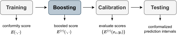
Figure 1: Illustration of the boosted conformal prediction procedure. We introduce a boosting stage between training and calibration, where we boost $\tau$ rounds on the conformity score function $E(\cdot,\cdot)$ and obtain the boosted score $E^{(\tau)}(\cdot,\cdot)$. The number of boosting rounds $\tau$ is selected via cross validation. A detailed description of the procedure is presented in Algorithm 1.

2 The split conformal procedure

We begin by outlining the key steps of the split conformal procedure applied to a family $\{(X_{i},Y_{i})\}_{i=1}^{n}$ of exchangeable samples (e.g., i.i.d.).

• Training. Randomly partition $[n]$ into a training set $I_{1}$ and a calibration set $I_{2}$. On the training set, train a model by means of an algorithm $\mathbbm{A}$ to produce a conformity score function $E(\cdot,\cdot;f)$. The structure of this score function is predetermined, whereas the model $f$ is learned from $\mathbbm{A}$. An example of a conformity score is $E(x,y;f)=|y-\hat{\mu}(x)|$, where $\hat{\mu}(x)$ is a learned regression function so that $f$ is here simply $\hat{\mu}$.

• Calibration. Evaluate the function $E(\cdot,\cdot;f)$ on each instance in the calibration set and obtain scores $\{E_{i}\}_{i\in I_{2}}$, with each $E_{i}=E(X_{i},Y_{i};f)$. The $(1-\alpha)$th empirical quantile of the score, $Q_{1-\alpha}(E,I_{2})$, is calculated as

  $$Q_{1-\alpha}(E,I_{2})=\inf\{z:\mathbbm{P}\left(Z\leq z\right)\geq 1-\alpha\},$$

  where $Z$ follows the distribution $\frac{1}{|I_{2}|+1}(\delta_{\infty}+\sum\delta_{E_{i}})$, and $\delta_{a}$ is a point mass at $a$.

• Testing. For a new observation $X_{n+1}$, output the conformalized prediction interval

  $${C_{n}}(X_{n+1})=\{y\in\mathbbm{R}:E(X_{n+1},y;f)\leq Q_{1-\alpha}(E,I_{2})\}.$$ (1)

If ties between $\{E_{i}\}_{i\in I_{2}}$ occur with probability zero, it holds that

$$1-\alpha\leq\mathbbm{P}(Y_{n+1}\in{C_{n}}(X_{n+1}))\leq 1-\alpha+\frac{2}{|I_{2}|+2},$$

see [16]. By introducing additional randomization during the calibration step, the prediction interval can be tuned to obey $\mathbbm{P}(Y_{n+1}\in{C_{n}}(X_{n+1}))=1-\alpha$, see [4]. This adjustment is not critical here and we omit the details.

Locally adaptive conformal prediction (Local for short) [16] introduces a score function that aims to make conformal prediction adapt to situations where the spread of the distribution of $Y$ varies significantly with the observed features $X$. On the training set, run an algorithm $\mathbbm{A}$ to fit two functions $\mu_{0}(\cdot)$ and $\sigma_{0}(\cdot)$, where $\mu_{0}(X)$ estimates the conditional mean $\mathbb{E}[Y\mid X]$, and $\sigma_{0}(X)$ the dispersion around the conditional mean, frequently chosen as the conditional mean absolute deviation (MAD), $\mathbb{E}[|Y-\mu_{0}(X)|\mid X]$. With $f=(\mu_{0},\sigma_{0})$, the locally adaptive (Local) score function is:

$$E(x,y;f)=|y-\mu_{0}(x)|/\sigma_{0}(x).$$ (2)

For a new observation $X_{n+1}$, the conformalized prediction interval (1) takes on the simplified expression $[{\mu}_{0}(X_{n+1})-{Q}_{1-\alpha}(E,I_{2}){\sigma}_{0}(X_{n+1}),{\mu}_{0}(X_{n+1})+{Q}_{1-\alpha}(E,I_{2}){\sigma}_{0}(X_{n+1})]$.

Conformalized quantile regression (CQR) [17] also aims to adapt to heteroskedasticity by calibrating conditional quantiles, which often results in shorter prediction intervals. Apply quantile regression to produce a pair of estimated quantiles $(\hat{q}_{\alpha/2}(x),\hat{q}_{1-\alpha/2}(x))$, where $\hat{q}_{\beta}(X)$ is the estimated $\beta$th quantile of the conditional distribution of $Y$. The CQR score function is defined as

$$E(x,y;f)=\max\{\hat{q}_{\alpha/2}(x)-y,y-\hat{q}_{1-\alpha/2}(x)\},$$ (3)

where $f=(\hat{q}_{\alpha/2},\hat{q}_{1-\alpha/2})$. For a new observation $X_{n+1}$, following (1) yields the prediction interval

$$\left[\hat{q}_{\alpha/2}(X_{n+1})-{Q}_{1-\alpha}(E,I_{2}),\hat{q}_{1-\alpha/2}(X_{n+1})+{Q}_{1-\alpha}(E,I_{2})\right].$$ (4)

Generalized conformity score families. To construct a Local conformity score, we estimate two functions $\mu_{0}(\cdot)$ and $\sigma_{0}(\cdot)$ to plug into (2). Since these components are constructed without looking at performance downstream, it is reasonable to imagine that other choices may enjoy enhanced properties. How then should we systematically select $\mu(\cdot)$ and $\sigma(\cdot)$? To address this, we define a generalized Local score family $\mathcal{F}$ containing all potential score functions of the form

$$\mathcal{F}:=\{E(\cdot,\cdot{;f}):E(x,y;f)=|y-\mu{(x)}|/\sigma(x),\sigma(\cdot)>0\},$$ (5)

where $f=(\mu,\sigma)$. For each $E(\cdot,\cdot{;f})\in\mathcal{F}$, the conformalized prediction interval is given by

$$\left[{\mu}(X)-{Q}_{1-\alpha}(E,I_{2}){\sigma}(X),{\mu}(X)+{Q}_{1-\alpha}(E,I_{2}){\sigma}(X)\right].$$ (6)

Turning to CQR, one notable limitation is the uniform adjustment of prediction intervals by the constant factor ${Q}_{1-\alpha}(E,I_{2})$, as shown in (4). This approach is suboptimal in the presence of heteroskedasticity, as it applies an identical correction to prediction intervals of varying widths for each $X=x$. Thus, simply updating the fitted quantiles $(\hat{q}_{\alpha},\hat{q}_{1-\alpha/2})$ and plugging them into the original score function would be inadequate, as the structure of the original score imposes significant limitations on the effectiveness of conformalized prediction intervals. To address this, several variants including CQR-m [22] and CQR-r [23] have been proposed. Focusing on CQR-r, it employs a flexible score function, defined as $E(x,y;f)=\max\{\hat{q}_{\alpha/2}(x)-y,y-\hat{q}_{1-\alpha/2}(x)\}/(\hat{q}_{1-\alpha/2}(x)-\hat{q}_{\alpha/2}(x))$, with $f=(\hat{q}_{\alpha/2},\hat{q}_{1-\alpha/2},\hat{q}_{1-\alpha/2}-\hat{q}_{\alpha/2})$. Following (1), conformalized prediction intervals become

$$\left[\hat{q}_{\alpha/2}(X)-\hat{\sigma}(X){Q}_{1-\alpha}(E,I_{2}),\hat{q}_{1-\alpha/2}(X)+\hat{\sigma}(X){Q}_{1-\alpha}(E,I_{2})\right],$$ (7)

where $\hat{\sigma}=\hat{q}_{1-\alpha/2}-\hat{q}_{\alpha/2}$. Intuitively, the adjusted score function allows prediction bands to adjust in proportion to their width, instead of adding a constant shift as in CQR. However, despite the intuitive appeal of adjusted scores as a seemingly more reasonable “allocation” of the conformal correction, empirical studies reveal that they do not result in narrower prediction intervals when compared to CQR [23]. This phenomenon is largely due to the uniform direction of the conformal adjustment, represented by ${Q}_{1-\alpha}(E,I_{2})$, across all observations. In particular, if ${Q}_{1-\alpha}(E,I_{2})<0$, indicating that the true target $y$ predominantly lies within the estimated quantile range $[\hat{q}_{\alpha/2},\hat{q}_{1-\alpha/2}]$, there is a uniform narrowing of the predicted interval across all samples.

In light of these insights, we propose a novel score family, $\mathcal{H}$, designed to augment the flexibility of the conformity score functions:

$$\mathcal{H}:=\bigl{\{}E(\cdot,\cdot{;f}):E(x,y{;f})=\max\left\{{\mu_{1}}(x)-y,y-\mu_{2}(x)\right\}/{\sigma}(x),\mu_{1}(\cdot)\leq\mu_{2}(\cdot),\sigma(\cdot)>0\bigr{\}},$$ (8)

where $f=(\mu_{1},\mu_{2},\sigma)$, which leads to conformalized prediction intervals of the form

$$[{\mu_{1}}(X) -{\sigma}(X){Q}_{1-\alpha}(E,I_{2}),{\mu_{2}}(X)+{\sigma}(X){Q}_{1-\alpha}(E,I_{2})].$$ (9)

Notably, $\mathcal{H}$ includes the Local, CQR, and CQR-r scores as special cases.

3 Boosted conformal procedure

It is clear from above that a model is trained to produce a conformity score $E(\cdot,\cdot;f)$; e.g., we may learn a regression function $\hat{\mu}(\cdot)$ to plug it into a score function $|y-\hat{\mu}(x)|$. To overcome the limitation of working with an arbitrarily selected score function, we introduce a boosting step before calibration, see Figure 1. In a nutshell, we use gradient boosting to iteratively improve upon a predefined score $E(\cdot,\cdot;f)$ now denoted as $E^{(0)}(\cdot,\cdot)$, where the superscript indicates the $0$th iteration.

To achieve this, we construct a task-specific loss function $\ell$, which takes a dataset $\mathcal{D}$ and a score function $E(\cdot,\cdot{;f})$ as inputs, and outputs $\ell(E(\cdot,\cdot{;f});\mathcal{D})$ measuring how closely the conformalized prediction interval aligns with the analyst’s objective. This loss function $\ell$ is designed to be differentiable with respect to each of the model components produced by the training algorithm. Importantly, it does not require knowledge of the gradient of $f(x)$ with respect to $x$. In the example above, taking the labels as fixed, this means that for each feature $x_{i}\in\mathcal{D}$, $i=1,\ldots,n$, if we set $\hat{y}_{i}=\hat{\mu}(x_{i})$, then the loss $\ell(E(\cdot,\cdot);\mathcal{D})$ is a function of $\{\hat{y}_{i}\}_{i=1}^{n}$, and the derivative $\partial\ell(E(\cdot,\cdot);\mathcal{D})/\partial\hat{y}_{i}$ is well defined. In Sections 5.1 and 6.1, we present examples of such derivatives.

Each boosting iteration updates the score function sequentially, employing a gradient boosting algorithm such as XGBoost [12] or LightGBM [15]. These algorithms accept as input a dataset $\mathcal{D}$, a base score function $E(\cdot,\cdot;f)$, a custom loss function $\ell$, gradients of $\ell$ with respect to $f$ (denoted $\nabla_{f}\ell$), and a number of boosting rounds $\tau$. We may write the boosting procedure as

$$(E^{(0)}(\cdot,\cdot),\ldots,E^{(\tau)}(\cdot,\cdot))=\text{GradientBoosting}(\mathcal{D},E(\cdot,\cdot;f),\ell,\nabla_{f}\ell,\tau).$$ (10)

This yields a boosted score function $E^{(\tau)}(\cdot,\cdot)$, which is then used for calibration and for constructing prediction intervals. The number $\tau$ is calculated using $k$-fold cross-validation on the training dataset, selecting $\tau$ from potential values up to a predefined maximum $T$ (e.g., 500). We partition the dataset into $k$ folds and for each $j=1,\ldots,k$, we hold out fold $j$ for sub-calibration and the remaining $k-1$ folds for sub-training. We apply $T$ rounds of gradient boosting (10) on the sub-training data, generating $T+1$ candidate score functions $E_{j}^{(0)}(\cdot,\cdot),\ldots,E_{j}^{(T)}(\cdot,\cdot)$. Each score function is then evaluated on sub-calibration data, using the loss function $\ell$ to compute losses at all epochs, i.e., for each fold $j=1,\ldots k$,

$$\{L_{j}^{(t)}\}_{t=0}^{T}=\{\ell(E_{j}^{(t)};\text{fold}_{j})\}_{t=0}^{T}.$$

Last, $\tau$ is selected as the round that minimizes the average loss across all $k$ folds:

$$\tau=\arg{\textstyle\min}_{0\leq t\leq T}{\textstyle\sum}_{j=1}^{k}L_{j}^{(t)},$$ (11)

see Figure 2. This cross-validation step simulates the calibration step in conformal prediction and effectively prevents the overfitting of the score function.

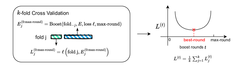
Figure 2: Schematic drawing showing the selection of the number of boosting rounds via cross-validation. Left: we hold out fold $j$, and use the remaining $k-1$ folds to generate candidate scores $E_{j}^{(t)}$, $t=0,\ldots,\text{max-round}$. The performance of each score is evaluated on fold $j$ using the loss function $\ell$. Right: best-round minimizes the average loss across all $k$ folds. A detailed description of the procedure is presented in Algorithm 1.

Searching within generalized conformity score families. To update the Local score function (2), we search within the generalized score family $\mathcal{F}$ (5). First, we initialize $\mu^{(0)}=\mu_{0}$ and $\sigma^{(0)}=\sigma_{0}$. After completing $\tau$ iterations of boosting on the training set, we obtain the boosted score function $E^{(\tau)}(x,y)=|y-\mu^{(\tau)}(x)|/\sigma^{(\tau)}(x)$. Notably, we can update any score function within $\mathcal{F}$. For instance, to update $E(x,y;f)=|y-\hat{\mu}(x)|$, we simply initialize $\mu^{(0)}=\hat{\mu}$, and take $\sigma^{(0)}$ to be the constant function equal to one. Similarly, to update the CQR score function (3), we search within the score family $\mathcal{H}$ (8). First, we initialize a triple $\mu_{1}^{(0)}=\hat{q}_{\alpha/2}$, $\mu_{2}^{(0)}=\hat{q}_{1-\alpha/2}$, $\sigma^{(0)}=\hat{q}_{1-\alpha/2}-\hat{q}_{\alpha/2}$. After $\tau$ boosting rounds, we obtain the boosted score function $E^{(\tau)}(x,y)=\max\{{\mu_{1}^{(\tau)}}(x)-y,y-{\mu_{2}}^{(\tau)}(x)\}/{\sigma}^{(\tau)}(x)$.

Algorithm 1 Boosting stage

Input:

$\text{Training data }(X_{i},Y_{i})\in\mathbbm{R}^{p}\times\mathbbm{R}$, $i=1,...,n$; base conformity score function $E^{(0)}(\cdot,\cdot)$

Loss function $\ell$; target mis-coverage level $\alpha\in(0,1)$

Number $k$ of cross-validation folds; maximum boosting rounds $T$

Procedure:

Randomly divide $\{1,...,n\}$ into $k$ folds

for $j\leftarrow 1$ to $k$ do

     Set fold $j$ as sub-calibration set, and the remaining $k-1$ folds as sub-training set

     On the sub-training set, call GradientBoosting (10) to obtain candidate scores $\{E_{j}^{(t)}\}_{t=0}^{T}$

     On the sub-calibration set, evaluate $L_{j}^{(t)}=\ell(E_{j}^{(t)})$, $t=0,\ldots,T$

end for

Set boosting rounds $\tau\leftarrow\arg\min_{t}\frac{1}{k}\sum_{j=1}^{k}L_{j}^{(t)}$ as in (11)

On the training set, call GradientBoosting (10) to obtain boosted functions $\{E_{j}^{(t)}\}_{t=0}^{\tau}$

Output:

Boosted conformity score function $E^{(\tau)}(\cdot,\cdot)$

4 Related Works

Adapting the classical conformal procedure to improve properties of the conformalized intervals has been one of the primary focuses of recent literature. Noteworthy contributions—including CF-GNN [28] and ConTr [26]—approach this problem by introducing modifications to the training stage of the procedure. As outlined in Section 2, a model is trained to produce a score function $E(\cdot,\cdot;f)$. The model $f$ usually depends on a set of model parameters, e.g., neural network parameters $\theta$. Denote the trained model $f$ by $f_{\theta}$. CF-GNN and ConTr retrain or fine-tune the model by using a carefully constructed loss function, which may aim to produce narrower prediction intervals or prediction sets of reduced cardinality in classification problems. This process generates a new set of model parameters $\theta^{\prime}$. The new model $f_{\theta^{\prime}}$ is then plugged into the same predefined conformity score function—namely CQR [28] or the adaptive prediction set score (APS) [26]—to produce $E(\cdot,\cdot,f_{\theta^{\prime}})$.

There are two primary limitations. First, the score function imposes constraints on the properties of conformalized intervals as explained in Section 2. Our approach introduces more flexibility by constructing a family of generalized score functions that is a superset of $\{E(\cdot,\cdot;f_{\theta}):\theta\in\Theta\}$, where $\Theta$ is the parameter space of the training model. This family is strategically designed to contain an oracle conformity score ideally suited to the task at hand, e.g., achieving exact conditional coverage. Second, current methodologies necessitate fine-tuning or retraining models from scratch, requiring both access to the training model and significant computational resources. In contrast, our boosted conformal method operates directly on model predictions and circumvents these issues.

Conditional coverage of conformalized prediction intervals has also attracted significant interest, characterized by efforts to establish theoretical guarantees and achieve numerical improvements. Prior work established an impossibility result [8, 20], which states that exact conditional coverage in finite samples cannot be guaranteed without making assumptions about the data distribution. Subsequently, Gibbs et al. [27] developed a modified conformal procedure that guarantees conditional coverage for predefined protected sub-groups, i.e. subsets of the feature space. Our approach differs from the previous works by introducing a numerical method directly aimed at improving the conditional coverage, $\mathbbm{P}(Y\in{C_{n}(}X)|X=x)$, across all potential values of $x$.

5 Boosting for conditional coverage

Maintaining valid marginal coverage, our goal is to produce a prediction interval ${C_{n}}$ obeying

$$\mathbbm{P}(Y\in{C_{n}}(X_{n+1})|X_{n+1}=x)\approx 1-\alpha$$ (12)

for all possible values of $x$. To this end, we present a loss function that quantifies the conditional coverage rate of any prediction interval. Requiring merely a dataset $\mathcal{D}$ and a prediction interval ${C_{n}(\cdot)}$ as inputs, it also serves as an effective evaluation metric, which may be of independent interest.

5.1 A measure for deviation from target conditional coverage

From now on, we let $E$ be the score function $E(\cdot,\cdot;f)$. Set $\mathcal{D}=\{(X_{i},Y_{i})\}_{i=1}^{n}$ and denote by ${C_{n}(\cdot)}$ the conformalized prediction interval constructed from ${E}$. We shall assess the deviation of ${C_{n}(\cdot)}$ from the target conditional coverage by means of Contrast Trees [21]. As background, a contrast tree iteratively identifies splits within the feature space $\mathcal{X}$ in a greedy fashion, aiming to maximize absolute within-group deviations from the target conditional coverage rate $(1-\alpha)$. For a subset $R$ of the data point indices $[n]$, let $\mathcal{D}_{R}=\{X_{j},Y_{j}\}_{j\in{R}}$. The absolute within-group deviation is computed as

$$d\left({C_{n}(\cdot)};\mathcal{D}_{{R}}\right)=\left|{|{R}|}^{-1}{\textstyle\sum}_{j\in{R}}\mathbbm{1}(Y_{j}\in{C_{n}(}X_{j}))-(1-\alpha)\right|.$$ (13)

The overall empirical maximum deviation is then defined as

$$\ell_{M}\left({E};\mathcal{D}\right)={\textstyle\max}_{1\leq m\leq M}{d\left({C_{n}(\cdot)};\mathcal{D}_{\hat{R}_{m}}\right)},$$ (14)

where $\hat{R}_{1}\cup\dots\cup\hat{R}_{M}$ is a partition of $[n]$, which itself depends on $E$ and $\mathcal{D}$. Specifically, it is computed by running a contrast tree for $M$ iterations. At each iteration, the algorithm not only seeks to isolate regions with large deviations but also discourages splits where any subset $\hat{R}_{m}$ is too small.

To update score functions via gradient boosting as described in (10), we would need a differentiable approximation of the maximum deviation. To this end, we construct approximations for the following three components of the loss function. With an abuse of notation, in subsequent discussions, we shall employ the same notations to denote these differentiable approximations.

1. Approximation for the prediction interval ${C_{n}(\cdot)}$ in (13): the prediction interval is formulated as (6) for the generalized Local score, and as (9) for the generalized CQR score. Denote the upper and lower limits of ${C_{n}(\cdot)}$ by $u(\cdot)$ and $l(\cdot)$. We approximate the empirical quantile $Q_{1-\alpha}(E,I_{2})$ in $u(\cdot)$ and $l(\cdot)$ with a smooth quantile estimator $Q^{s}_{1-\alpha}$. Given $r$ scalars $\{z_{i}\}_{i=1}^{r}$, ${Q^{s}_{1-\alpha}}$ is constructed as:

   $${Q^{s}_{1-\alpha}}(\{z_{i}\}_{i=1}^{r}):=\langle\text{HD}(r),s(\mathbf{z})\rangle,$$ (15)

   where $\langle\cdot,\cdot\rangle$ represents the dot product. Here, $\text{HD}(r)=[W_{r,1},...,W_{r,r}]$ is the weight vector corresponding to the Harrel-Davis distribution-free empirical quantile estimator [1], and $s(\mathbf{z})$ is a differentiable ordering $\{\tilde{z}_{(i)}\}_{i=1}^{r}$, arranged in the ascending order. In practice, the derivative of $s(\textbf{z})$ with respect to each $z_{i}$ is given by the package developed in [19]. This approach is a smooth approximation of the Harrel-Davis quantile estimator $Q^{\text{HD}}_{1-\alpha}$, constructed as a linear combination of the order statistics, $Q^{\text{HD}}_{1-\alpha}=\langle\text{HD}(r),\{z_{(i)}\})\rangle={\textstyle\sum}_{i=1}^{r}W_{r,i}z_{(i)}$, where $W_{r,i}$ takes the value $I_{(1-\alpha)(r+1),\alpha(r+1)}(i/r)-I_{(1-\alpha)(r+1),\alpha(r+1)}((i-1)/r)$ and $I_{a,b}(x)$ represents the incomplete beta function.

2. Approximation for absolute deviation $d_{i}$ (13): the indicator function in (13) can be approximated by the product of two sigmoid functions,

   $$\mathbbm{1}(Y_{j}\in{C_{n}}(X_{j})) =\mathbbm{1}({u}(X_{j})-Y_{j}\geq 0)\mathbbm{1}(Y_{j}-{l}(X_{j})\geq 0)$$

   $$\approx S_{\tau_{1}}({u}(X_{j})-Y_{j})S_{\tau_{1}}(Y_{j}-{l}(X_{j})),$$

   where $\tau_{1}$ is a parameter, trading off smoothness and quality of the approximation. The sigmoid function $S_{\tau_{1}}(x)$ is defined as $S_{\tau_{1}}(x)=(1+e^{-\tau_{1}x})^{-1}$.

3. Approximation for maximum deviation: we employ a log-sum-exp function [2] to derive the differentiable approximation of $\ell_{M}$ as

   $${\ell}_{M}\left({E};\mathcal{D}\right):={\tau_{2}}^{-1}\log{\textstyle\sum}_{m=1}^{M}\exp{\left(\tau_{2}{d}_{m}({C_{n}}(\cdot);\mathcal{D}_{m})\right)},$$ (16)

   where $\tau_{2}$ is a parameter, serving the same purpose as $\tau_{1}$.

Here, we demonstrate calculating the derivative of the smooth approximation (16) with respect to each component of the generalized Local score, expanding it as follows:

$${\ell}_{M}\left({E};\mathcal{D}\right)={\tau_{2}}^{-1}\log\sum_{m=1}^{M}\exp{\left(\tau_{2}\left|{|R_{m}|}^{-1}{\textstyle\sum}_{j\in R_{m}}S_{\tau_{1}}({u}(X_{j})-Y_{j})S_{\tau_{1}}(Y_{j}-{l}(X_{j}))-(1-\alpha)\right|\right)},$$

where

$$S_{\tau_{1}}({u}(X_{j})-Y_{j})=\left(1+\exp\left[-\tau_{1}(\mu_{j}+{Q}_{1-\alpha}^{s}(\{E_{i}\}_{i=1}^{n})\sigma_{j}-Y_{j})\right]\right)^{-1},$$

$$S_{\tau_{1}}(Y_{j}-{l}(X_{j}))=\left(1+\exp\left[-\tau_{1}(Y_{j}-\mu_{j}+{Q}_{1-\alpha}^{s}(\{E_{i}\}_{i=1}^{n})\sigma_{j})\right]\right)^{-1},$$

with $\mu_{i}=\mu(X_{i})$, $\sigma_{i}=\sigma(X_{i})$, $E_{i}=|Y_{i}-\mu_{i}|/\sigma_{i}$. As a result, for each feature $X_{i}$ within $\mathcal{D}$, we can evaluate $\partial{\ell}_{M}\left({E};\mathcal{D}\right)/\partial\mu_{i}$ and $\partial{\ell}_{M}\left({E};\mathcal{D}\right)/\partial\sigma_{i}$ via the chain rule.

5.2 Boosting score functions for conditional coverage

Since the empirical maximum deviation $\ell_{M}$ (14) is non-differentiable, we opt for the differentiable approximation during the gradient boosting step (10). Nonetheless, we utilize the original $\ell_{M}$ to select the number of boosting rounds as in step (11) and to evaluate the conditional coverage of the conformalized prediction interval on the test set.

5.2.1 Theoretical guarantees

The oracle score function achieving conditional coverage as defined in (12) belongs to both proposed generalized score families.

Theorem 5.1 (Asymptotic expressiveness).

Let $\{X_{i},Y_{i}\}_{i=1}^{n}$ be i.i.d. with continuous joint probability density distribution. Under the split conformal procedure, for any target coverage rate $1-\alpha$, as $n\rightarrow\infty$, there exists $(\mu^{*},\sigma^{*})$ and $(\mu_{1}^{*},\mu_{2}^{*},\sigma^{*})$ such that the corresponding generalized Local (5) and CQR (8) score functions recover conditional coverage at rate $1-\alpha$, as defined in (12).

It goes without saying that there is no reason to assume that the optimal $\mu^{*}$ corresponds to the conditional mean, median or any quantile of $Y$ given $X$, or that the optimal $\sigma^{*}$ corresponds to the standard deviation or the mean absolute deviation of $Y$ given $X$, as in the original Local score (2). That said, our greedy strategy has no guarantee on global optimality and this is why the choice of the starting point—whether it is the Local or CQR score function—plays a role in the performance.

5.2.2 Empirical results on real data

We apply our boosted conformal procedure to the 11 datasets previously analyzed in [23, 18, 22]. Details on the datasets are provided in Section A.6 in the Appendix. In each dataset, we randomly hold out $20\%$ as test data. All experiments are repeated 10 times, starting from the data splitting. We refer to Section A.7 for details on the models and hyper-parameters we employ for the training and boosting stages.

We evaluate the conditional coverage of the prediction intervals as the maximum within-group deviations across a partitioned test set (14). This partition is obtained through a contrast tree algorithm described in Section 5.1. Figure 3 illustrates the comparison between miscoverage rates of prediction intervals at each leaf of the contrast tree. These intervals are derived under the classical Local conformal procedure and our boosted conformal procedure. Notably, the conditional coverage of the boosted prediction interval more closely aligns with the target rate $1-\alpha$.

The experiment results summarized in Table 1 indicate that applying boosting significantly enhances the performance of the baseline Local procedure. In contrast, boosting on CQR does not yield significant improvements—a sign that CQR already targets conditional coverage. (Before boosting, the prediction intervals generated by the baseline Local procedure exhibit conditional coverage deviations up to three times greater than those of the baseline CQR procedure.) It is noteworthy, however, that after boosting, the conditional coverage of the Local procedure improves to a level comparable to that of the boosted CQR procedure. While generally slightly less effective, nevertheless surpasses the performance of the boosted CQR procedure in two cases. Results on the remaining datasets are deferred to Table A2.

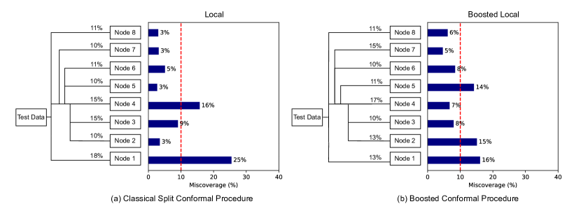
Figure 3: Comparison of test set conditional coverage evaluated on the dataset meps-19: (a) shows the classical Local-type conformal procedure and (b) our boosted Local-type conformal procedure. The target miscoverage rate is set to $\alpha=10\%$ (red). Miscoverage rate is computed at each leaf of the contrast tree, constructed to detect deviation from the target rate. Each leaf node is labeled with its size, namely, the fraction of the test set it represents.

Table 1: Test set maximum deviation loss $\ell_{M}$ evaluated on various conformalized intervals. The best result achieved for each dataset is highlighted in bold.

Max. Conditional Coverage Deviation ($\%$), target miscoverage $\alpha=10\%$
Dataset	Method		Improvement	Method		Improvement
	Local	Boosted		CQR	Boosted
bike	$10.979\,432$	5.638	$\text{-48.65}\%$	$4.933\,807$	4.925	-0.17%
bio	$5.303\,131$	4.862	$\text{-8.31}\%$	$5.068\,905$	4.700	-7.29%
community	$25.754\,902$	13.466	$\text{-47.71}\%$	$12.687\,841$	12.105	-4.59%
concrete	$10.739\,634$	8.763	$\text{-18.40}\%$	$9.038\,694$	8.265	-8.56%
meps-19	$15.357\,278$	5.656	$\text{-63.17}\%$	$5.506\,775$	5.507	-0.00%
meps-20	$16.938\,720$	6.998	$\text{-58.69}\%$	$7.614\,116$	7.184	-5.65%
meps-21	$17.627\,239$	7.832	$\text{-55.57}\%$	$8.164\,735$	8.067	-1.2%

6 Boosting for length/power

We begin by specifying the oracle prediction interval with minimum length. For a random variable $Z$, the High Density Region (HDR) at a specified significance level $\alpha$, denoted as $\text{HDR}_{\alpha}(Z)$, is defined as the shortest deterministic interval that covers $Z$ with probability at least $1-\alpha$. The boundaries of $\text{HDR}_{\alpha}(Z)$, the lower limit $Q_{l(\alpha)}$ and the upper limit $Q_{u(\alpha)}$, obey the condition $\mathbbm{P}(Z\in[Q_{l(\alpha)},Q_{u(\alpha)}])\geq 1-\alpha$. For a pair of $(X,Y)$ drawn from $P$, for every value of $x\in\mathbb{R}^{p}$, the most powerful oracle prediction interval at that point is expressed as

$$\text{HDR}_{\alpha}(Y|X=x)=\left[Q_{l(\alpha)}(Y|X=x),Q_{u(\alpha)}(Y|X=x)\right].$$ (17)

Before introducing the strategy to boost power, we present a word of caution against optimizing exclusively for this objective. Importantly, to maintain valid marginal coverage, the most powerful prediction interval is prone to overcover when the spread of $Y|X$ (the conditional distribution of $Y$ given $X$) is small, and undercover when the spread of $Y|X$ is large. This may be undesirable.

Similar to Theorem 5.1, we can show that the generalized score families exhibit the necessary expressiveness to contain the oracle conformity score, achieving optimal length while ensuring valid marginal coverage. The formal theorem is deferred to Section A.3.

6.1 A measure for length/power

Consider a dataset $\mathcal{D}=\{(X_{i},Y_{i})\}_{i=1}^{n}$ and a score function ${E}$. Denote the corresponding conformalized prediction interval by ${C_{n}(\cdot)}$, with its quality measured by the average length:

$$\ell_{P}({E};\mathcal{D})=n^{-1}{\textstyle\sum}_{i=1}^{n}|{C_{n}(}X_{i})|.$$ (18)

To derive a differentiable approximation of ${\ell}_{P}$, we approximate the empirical quantile $Q_{1-\alpha}$ in the conformalized intervals (6) and (9) with the smooth quantile estimator ${Q^{s}_{1-\alpha}}$ constructed in (15). Here, we demonstrate calculating the derivative of the smooth approximation of ${\ell}_{P}$ with respect to each component of the generalized Local score, expanding it as follows based on the previously outlined approximation steps:

$${\ell}_{P}\left({E};\mathcal{D}\right)=2\bar{\sigma}{Q}_{1-\alpha}^{s}(\{E_{i}\}_{i=1}^{n}),\qquad E_{i}=|Y_{i}-\mu_{i}|/\sigma_{i},$$

with $\mu_{i}=\mu(X_{i})$, $\sigma_{i}=\sigma(X_{i})$, $\bar{\sigma}=n^{-1}\sum_{i=1}^{n}\sigma_{i}$. As a result, for each feature $X_{i}$ within $\mathcal{D}$, we can evaluate $\partial{\ell}_{P}\left({E};\mathcal{D}\right)/\partial\mu_{i}$ and $\partial{\ell}_{P}\left({E};\mathcal{D}\right)/\partial\sigma_{i}$ via the chain rule. For instance,

$${\partial{\ell}_{P}\left({E};\mathcal{D}\right)}/{\partial\mu_{i}}=-2\bar{\sigma}[{\partial{Q}_{1-\alpha}^{s}(\{E_{j}\}_{j=1}^{n})}/{\partial E_{i}}]\cdot[{\text{sign}(Y_{i}-\mu_{i})}/{\sigma_{i}}].$$

6.2 Empirical results on real data

We apply our boosted conformal procedure to the same datasets described in Section 5.2.2. Detailed information on the models and hyperparameters used during the training and boosting stages can be found in Section A.7. Partial experiment results are summarized in Table 2. Notably, the boosting performance highlighted in bold exhibits significant improvement compared to previously documented results [17, 23]. We see a pronounced enhancement with the blog dataset; before boosting, the Local prediction intervals are on average $47\%$ longer than those generated by CQR. After boosting, these intervals outperform the boosted CQR intervals by $20\%$. Using CQR as the baseline also yields substantial improvements, a decrease in averaged length exceeding $10\%$ in six out of the eleven datasets. The meps-21 dataset, in particular, shows an improvement of up to $17\%$ relative to the baseline. Results on the remaining datasets can be found in Table A3. Figure 4 compares the conformalized prediction intervals derived from baseline Local and CQR scores with those obtained from the boosted scores. To effectively visualize the impact of boosting, we conduct a regression tree analysis on the training set to predict the label $Y$, setting the maximum number of tree nodes to four. This regression tree is then applied to the test set, allowing for a detailed comparison of the prediction intervals across each of the four distinct leaves.

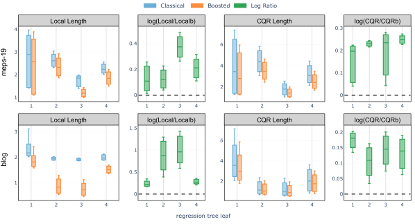
Figure 4: Comparison of test set power (averaged interval length) evaluated on the meps-19 and blog datasets: classical Local and CQR conformal procedure versus the boosted procedures (abbreviated as ‘Localb’ and ‘CQRb’) compared in each of the 4 leaves of a regression tree trained on the training set to predict the label $Y$. A positive log ratio value between the regular and boosted interval lengths indicates improvement from boosting. The target miscoverage rate is set at $\alpha=10\%$.

Table 2: Test set power $\ell_{P}$ evaluated on various conformalized prediction intervals. The best result achieved for each dataset is highlighted in bold.

Power Loss (Average Length), target miscoverage $\alpha=10\%$
Dataset	Method		Improvement	Method		Improvement
	Local	Boosted		CQR	Boosted
blog	$2.056\,256$	1.068	$\text{-48.08}\%$	$1.395\,251$	1.382	$\text{-0.93}\%$
facebook-1	$1.896\,465$	1.443	$\text{-18.76}\%$	$1.184\,559$	1.056	$\text{-10.85}\%$
facebook-2	$1.854\,089$	1.319	$\text{-28.87}\%$	$1.220\,906$	1.055	$\text{-13.57}\%$
meps-19	$2.070\,403$	1.695	$\text{-18.15}\%$	$2.553\,117$	2.205	$\text{-13.64}\%$
meps-20	$2.081\,153$	1.836	$\text{-12.26}\%$	$2.668\,877$	2.346	$\text{-12.09}\%$
meps-21	$2.062\,927$	1.805	$\text{-12.49}\%$	$2.620\,299$	2.173	$\text{-17.06}\%$

7 Discussion

We introduced a post-training conformity score boosting scheme aiming to optimize for conditional coverage and power of the conformalized prediction interval. An intriguing avenue for future exploration involves simultaneously optimizing both power and conditional coverage, potentially incorporating user-specified weights for these objectives. Additionally, we can readily adapt our procedure to meet various application-specific objectives. For instance, we can optimize for conditional coverage on predefined feature groups, a common task in enhancing fairness in distributing social resources across different demographic groups [27]. Similarly, we can modify our procedure to reduce the length of prediction intervals for predefined label groups, which can be seen as reallocating resources to decrease uncertainty for certain groups at the expense of higher uncertainty for other groups [26]. Candidate loss functions tailored to these objectives are detailed in Section A.1. Lastly, the primary emphasis of this paper centers on the design of the conformity score boosting scheme and formalizing the optimization of conditional coverage in mathematical terms, leaving room for computational optimization to enhance performance and runtime efficiency.

Appendix A Appendix

A.1 Candidate loss functions for additional application-specific objectives

Conditional coverage on predefined feature groups: this task can be viewed as a specialized application within our broader strategy of boosting for conditional coverage, as detailed in Section 5. There, the primary challenge was to develop a loss function that accurately measures deviations from the target conditional coverage rate. We achieved this by using contrast trees to identify partitions in the feature space that maximize these deviations, effectively identifying subgroups in need of protection. This process is simplified when the partitions correspond to prespecified groups, allowing us to continue using the empirical maximum deviation as a candidate loss function.

Consider a dataset $\mathcal{D}=\{(X_{i},Y_{i})\}_{i=1}^{n}$ and a score function ${E}$. Denote by ${C_{n}(}\cdot)$ the conformalized prediction interval constructed from ${E}$. Let $G_{1},\ldots,G_{M}$ be prespecified feature index groups. Within each set $\mathcal{D}_{i}=\{(X_{j},Y_{j})\}_{j\in G_{i}}$, compute the absolute deviation $d_{i}$ as

$$d_{i}\left({C_{n}(}\cdot);\mathcal{D}_{i}\right)=\left|\frac{1}{|G_{i}|}{\textstyle\sum}_{j\in G_{i}}\mathbbm{1}(Y_{j}\in{C_{n}(}X_{j}))-(1-\alpha)\right|.$$ (19)

The overall empirical maximum deviation is then defined as

$$\ell\left({E};\mathcal{D}\right)={\textstyle\max}_{1\leq i\leq M}{d_{i}\left({C_{n}(}\cdot);\mathcal{D}_{i}\right)}.$$ (20)

Interval length conditional on predefined label groups: for a dataset $\mathcal{D}=\{(X_{i},Y_{i})\}_{i=1}^{n}$ and a score function ${E}$, let $\mathcal{Y}_{1},\ldots,\mathcal{Y}_{M}$ be the prespecified label groups. A natural minimization objective for balancing uncertainty among these groups is defined as:

$$\ell({E};\mathcal{D})=\sum_{i=1}^{M}w_{i}\frac{1}{\sum_{j=1}^{n}\mathbbm{1}(Y_{j}\in\mathcal{Y}_{i})}\sum_{j=1}^{n}\mathbbm{1}(Y_{j}\in\mathcal{Y}_{i})|{C_{n}(}X_{j})|,$$

where $(w_{1},\ldots,w_{M})$ represents a set of user-specified weights.

A.2 Proof of Theorem 5.1

Our proof relies on the following lemma.

Lemma A.1 (Expressiveness).

Given any sample pair $X$ and $Y$ with a continuous joint probability density distribution, and a prediction interval $[c_{l}(\cdot),c_{u}(\cdot)]$ with marginal coverage equal to $1-\alpha$, there exist specific function sets: ($\mu(\cdot)$,$\sigma(\cdot)$) for the Local type, and ($\mu_{1}(\cdot)$,$\mu_{2}(\cdot)$,$\tilde{\sigma}(\cdot)$) for the CQR type, such that asymptotically:

1. The conformalized prediction interval (6), derived using the generalized Local type conformity score $f_{\mu,\sigma}$, accurately recovers $[c_{l}(\cdot),c_{u}(\cdot)]$.

2. Similarly, the conformalized prediction interval (9), based on the generalized CQR type conformity score $E_{\mu_{1},\mu_{2},\tilde{\sigma}}$, also recovers $[c_{l}(\cdot),c_{u}(\cdot)]$.

Proof of Lemma A.1.

Recall that the generalized Local score (5) characterized by $(\mu,\sigma)$ takes the form

$$E_{\mu,\sigma}(x,y)=\frac{|y-\mu{(x)}|}{\sigma(x)}.$$ (21)

Asymptotically, the conformalized prediction interval is given by

$$\left[{\mu}(X)-{Q}_{1-\alpha}(E_{\mu,\sigma}){\sigma}(X),{\mu}(X)+{Q}_{1-\alpha}(E_{\mu,\sigma}){\sigma}(X)\right].$$ (22)

Here, ${Q}_{1-\alpha}$ represents the population quantile. Set

$$\mu(x) =\frac{c_{l}(x)+c_{u}(x)}{2},\quad\sigma(x)=\frac{c_{u}(x)-c_{l}(x)}{2}.$$

By assumption, we have

$$\mathbbm{P}(Y\in[c_{l}(X),c_{u}(X)])=1-\alpha.$$

With a simple change of variables, the above inequality is equivalent to

$$\mathbbm{P}\left(\left|\frac{Y-\mu(X)}{\sigma(X)}\right|\leq 1\right)=1-\alpha.$$

In other words, this is equivalent to

$$Q_{1-\alpha}(E_{\mu,\sigma})=1.$$

We have thus proved the result for the generalized Local type conformity score $E_{\mu,\sigma}$. In the same spirit, we can prove the result for the generalized CQR type conformity score $E_{\mu_{1},\mu_{2},\tilde{\sigma}}$ by taking

$$\mu_{1}=c_{l}+\frac{c_{u}(x)-c_{l}(x)}{2},\quad\mu_{2}=c_{u}-\frac{c_{u}(x)-c_{l}(x)}{2},\quad\tilde{\sigma} =\frac{c_{u}(x)-c_{l}(x)}{2}.$$

Recall that a generalized CQR score function (8) characterized by ($\mu_{1}$, $\mu_{2}$, $\sigma$) is defined as:

$$E_{\mu_{1},\mu_{2},{\sigma}}(x,y)=\max\left\{{\mu_{1}}(x)-y,y-\mu_{2}(x)\right\}/{\sigma}(x),$$ (23)

which leads to the asymptotic conformalized prediction intervals of the form

$$[{\mu_{1}}(X) -{\sigma}(X){Q}_{1-\alpha}(E_{\mu_{1},\mu_{2},{\sigma}}),{\mu_{2}}(X)+{\sigma}(X){Q}_{1-\alpha}(E_{\mu_{1},\mu_{2},{\sigma}})].$$ (24)

Plugging in $\mu_{1}$, $\mu_{2}$, $\tilde{\sigma}$ defined above, we immediately have

$$\mathbbm{P}(Y\in[c_{l}(X),c_{u}(X)])=1-\alpha$$

$$\Longleftrightarrow\hskip 5.0pt \mathbbm{P}(c_{l}(X)-Y\leq 0,Y-c_{u}(X)\leq 0)=1-\alpha$$

$$\Longleftrightarrow\hskip 5.0pt \mathbbm{P}\left(\frac{c_{l}(X)-Y+\tilde{\sigma}(X)}{\tilde{\sigma}(X)}\leq 1,\frac{Y-c_{u}(X)+\tilde{\sigma}(X)}{\tilde{\sigma}(X)}\leq 1\right)=1-\alpha$$

$$\Longleftrightarrow\hskip 5.0pt Q_{1-\alpha}(E_{\mu_{1},\mu_{2},{\sigma}}(x,y))=1.$$

∎

Proof of Theorem 5.1.

It suffices to take $c_{l}(x)=Q_{\alpha/2}(Y|X=x)$, $c_{u}(x)=Q_{1-\alpha/2}(Y|X=x)$ and apply Lemma A.1. ∎

A.3 Boosting for length: theoretical guarantees

Similar to Theorem 5.1, we show in Theorem A.2 below that the generalized Local and CQR score families exhibit the necessary expressiveness to contain the oracle score, achieving optimal length while ensuring valid marginal coverage.

Theorem A.2 (Asymptotic expressiveness).

Under the assumptions of Theorem 5.1, for any target coverage rate $1-\alpha$, as $n\rightarrow\infty$, the following statements hold true:

1. There exists $(\mu^{*},\sigma^{*})$ such that the corresponding generalized Local score function (5) recovers the most powerful oracle prediction interval (17).

2. There exists $(\mu_{1}^{*},\mu_{2}^{*},\sigma^{*})$ such that the corresponding generalized CQR score function (8) recovers the most powerful oracle prediction interval (17).

Proof of Theorem A.2.

It suffices to take $c_{l}(x)=Q_{l(\alpha)}(Y|X=x)$, $c_{u}(x)=Q_{u(\alpha)}(Y|X=x)$ and apply Lemma A.1, where $Q_{l(\alpha)}$ and $Q_{u(\alpha)}$ are the lower and upper limits of the High Density Region defined in (17). ∎

A.4 CQR type conformity score boosting

A generalized CQR score function (8) is uniquely defined by a triple ($\mu_{1}(\cdot),\mu_{2}(\cdot),\sigma(\cdot)$). We will show how searching for a generalized CQR score can be reduced to searching for a Local generalized score. To begin with, we shall say that score functions are equivalent if they recover identical conformalized prediction intervals.

Definition A.3.

Let $\{X_{i},Y_{i}\}_{i=1}^{n}$, $(X_{n+1},Y_{n+1})$ be i.i.d. with continuous joint probability density distribution, and let $[n]$ be partitioned into a training set $I_{1}$ and a calibration set $I_{2}$. Consider two conformity score functions, $E_{1}$ and $E_{2}$, which produce conformalized prediction intervals $C_{1}(\cdot)$ and $C_{2}(\cdot)$, respectively. For any target coverage rate $1-\alpha$, $E_{1}$ and $E_{2}$ are equivalent if $C_{1}(\cdot)=C_{2}(\cdot)$ when marginal coverage rates $\mathbbm{P}(Y_{n+1}\in C_{1}(X_{n+1}))$ and $\mathbbm{P}(Y_{n+1}\in C_{2}(X_{n+1}))$ match.

Building on this definition, we are now equipped to establish the following equivalences:

Lemma A.4.

Under the assumptions of Definition A.3, the following statements hold:

1. For the CQR-r score function defined in Section 2, there is an equivalent generalized Local score function characterized by a pair $(\mu(\cdot),\sigma(\cdot))$, where $\mu=(\mu_{1}+\mu_{2})/2$, $\sigma=(\mu_{2}-\mu_{1})/2$.

2. For any generalized Local score function characterized by the pair $(\mu(\cdot),\sigma(\cdot))$, there is an equivalent generalized CQR score function characterized by a triple $(\mu(\cdot),\mu(\cdot),\sigma(\cdot))$.

The proof of the above Lemma is deferred to Section A.5. Leveraging these equivalences, we carry out the boosted conformal procedure as follows: first, we initialize a triple $\mu_{1}^{(0)}=\hat{q}_{\alpha/2}$, $\mu_{2}^{(0)}=\hat{q}_{1-\alpha/2}$, $\sigma_{1}^{(0)}=\hat{q}_{1-\alpha/2}-\hat{q}_{\alpha/2}$, which characterizes the CQR-r score function. Next, we find an equivalent generalized Local score function characterized by a pair $(\mu^{(0)},\sigma^{(0)})$ chosen according to Lemma A.4. After $\tau$ boosting rounds, we obtain the boosted pair $(\mu^{(\tau)},\sigma^{(\tau)})$ and the corresponding score function. Finally, we recover an equivalent generalized CQR score function

$$E^{(\tau)}(x,y)=\max\left\{{\mu_{1}^{(\tau)}}(x)-y,y-{\mu_{2}}^{(\tau)}(x)\right\}/{\sigma}_{1}^{(\tau)}(x),$$

characterized by the triple $({\mu_{1}}^{(\tau)},{\mu_{2}}^{(\tau)},{\sigma_{1}}^{(\tau)})$ chosen according to Lemma A.4.

A.5 Proof of Lemma A.4

Recall that the generalized Local score (5) characterized by $(\mu,\sigma)$ takes the form

$$E_{\mu,\sigma}(x,y)=\frac{|y-\mu{(x)}|}{\sigma(x)}.$$ (25)

The conformalized prediction interval is given by

$$\left[{\mu}(X)-{Q}_{1-\alpha}(E_{\mu,\sigma},I_{2}){\sigma}(X),{\mu}(X)+{Q}_{1-\alpha}(E_{\mu,\sigma},I_{2}){\sigma}(X)\right].$$ (26)

A generalized CQR score function (8) characterized by ($\mu_{1}$, $\mu_{2}$, $\sigma$) is defined as:

$$E_{\mu_{1},\mu_{2},{\sigma}}(x,y)=\max\left\{{\mu_{1}}(x)-y,y-\mu_{2}(x)\right\}/{\sigma}(x),$$

which leads to conformalized prediction intervals of the form

$$[{\mu_{1}}(X) -{\sigma}(X){Q}_{1-\alpha}(E_{\mu_{1},\mu_{2},{\sigma}},I_{2}),{\mu_{2}}(X)+{\sigma}(X){Q}_{1-\alpha}(E_{\mu_{1},\mu_{2},{\sigma}},I_{2})].$$

1. Plugging in the triple $\mu_{1}(x)=\hat{q}_{\alpha/2}$, $\mu_{2}(x)=\hat{q}_{1-\alpha/2}$, $\sigma_{1}(x)=\hat{q}_{1-\alpha/2}-\hat{q}_{\alpha/2}$, which characterize the CQR-r score function, we have the conformalized prediction interval

   $$[\mu_{1}(X)-\sigma_{1}(X){Q}_{1-\alpha}(E_{\mu_{1},\mu_{2},\sigma_{1}},I_{2}),\mu_{2}(X)+\sigma_{1}(X){Q}_{1-\alpha}(E_{\mu_{1},\mu_{2},\sigma_{1}},I_{2})].$$

   Set

   $$\mu(X)=\frac{\mu_{1}(X)+\mu_{2}(X)}{2},\sigma(X)=\frac{\mu_{2}(X)-\mu_{1}(X)}{2},$$

   then the generalized Local conformity score $E_{\mu,\sigma}(x,y)={|y-\mu(x)|}/{\sigma(x)}$ recovers conformalized prediction intervals of the form

   $$[\mu(X)-\sigma(X)Q(E_{\mu,\sigma},I_{2}),\mu(X)+\sigma(X)Q(E_{\mu,\sigma},I_{2})]$$

   $$= \left[\frac{\mu_{1}(X)+\mu_{2}(X)}{2}-\frac{\mu_{2}(X)-\mu_{1}(X)}{2}Q(E_{\mu,\sigma},I_{2}),\right.$$

   $$\left.\quad\quad\quad\quad\quad\quad\quad\quad\quad\quad\quad\quad\frac{\mu_{1}(X)+\mu_{2}(X)}{2}+\frac{\mu_{2}(X)-\mu_{1}(X)}{2}Q(E_{\mu,\sigma},I_{2})\right]$$

   $$= \left[\mu_{2}(X)-(\mu_{2}(X)-\mu_{1}(X))\frac{Q(E_{\mu,\sigma},I_{2})-1}{2},\right.$$

   $$\left.\quad\quad\quad\quad\quad\quad\quad\quad\quad\quad\quad\quad\mu_{1}(X)+(\mu_{2}(X)-\mu_{1}(X))\frac{Q(E_{\mu,\sigma},I_{2})-1}{2}\right]$$

   $$= \left[\mu_{1}(X)-\sigma_{1}(X)\frac{Q(E_{\mu,\sigma},I_{2})-1}{2},\mu_{2}(X)+\sigma_{1}(X)\frac{Q(E_{\mu,\sigma},I_{2})-1}{2}\right].$$

   From the monotonicity of the interval lengths with respect to the empirical quantiles, we have that the two score functions are equivalent by Definition A.3.

2. Let a generalized Local score function be $E_{\mu,\sigma}(x,y)=|y-\mu(x)|/\sigma(x)$. Then it suffices to observe that

   $$|y-\mu(x)|=\max\{y-\mu(z),\mu(x)-y\}.$$

A.6 Additional information on real datasets

In Table A1, we provide the predicted label, dimensions, and source for each dataset. Data cleaning and preprocessing are in accordance with the methods described by Romano et al. [17].

Table A1: Datasets for our empirical analyses, with the predicted label, number of samples ($n$), and features ($d$).

Name	Label	$n$	$d$	Source
bike	bike rental counts	10886	18	[9]
bio	deviation of predicted from native protein structure	45730	9	[10]
blog	number of comments in the next 24 hours	52397	280	[11]
community	crime rate per community	1994	100	[7]
concrete	concrete compressive strength	1030	8	[5]
facebook-1	Facebook comment volume	40948	53	[5]
facebook-2	Facebook comment volume	81311	53	[13]
meps-19	utilization of medical services	15785	139	[29]
meps-20	utilization of medical services	17541	139	[30]
meps-21	utilization of medical services	15656	139	[31]
star	total student test scores up to the third grade	2161	39	[6]

All datasets, except for the meps and star data sets, are licensed under CC-BY 4.0. The Medical Expenditure Panel Survey (meps) data is subject to copyright and usage rules. The licensing status of the star dataset could not be determined.

A.7 Experimental Setup

In each dataset, we randomly hold out $20\%$ as test data. The remaining data is divided into a training set and a calibration set, each taking up a proportion of $\gamma$ and $1-\gamma$. We explore training ratios $\gamma$ ranging from $10\%$ to $90\%$. Results corresponding to the optimal value of the hyperparameter $\gamma$ are recorded in Table 1, following the practice of Sesia er al. [23].

In the training stage, we employ the random forest regressor from Python’s scikit-learn package to learn the baseline Local score function. The hyperparameters are the package defaults, except for the total number of trees, which we set to 1000, and the minimum number of samples required at a leaf node, which we set to 40, as recommended by Romano et al. [17]. For the baseline CQR score function, we adopt a black-box neural network quantile regressor with three fully connected layers and ReLU non-linearities, following the practice of Sesia et al. [23]. In the boosting stage, we set the hyper-parameters $\tau_{1}$, $\tau_{2}$ in the approximated loss (16) to 50. The approximated loss is then passed to the Gradient Boosting Machine from Python’s XGBoost package along with a base conformity score. We set the maximum tree depth to 1 to avoid overfitting and perform cross-validation for the number of boosting rounds, as outlined in Section 3. All other hyperparameters are set to package defaults.

All experiments were conducted on a dual-socket AMD EPYC 7502 32-Core Processor system, utilizing 8 of its 128 CPUs each time. The runtime for each dataset and random seed varies by dataset size, ranging from 10 minutes to 5 hours.

A.8 Additional results and error bars

In Tables A2 and A3, we report additional experiment results for the datasets not included in Tables 1 and 2.

Table A2: Test set maximum deviation loss $\ell_{M}$ evaluated on various conformalized intervals.

Max. Conditional Coverage Deviation ($\%$), target miscoverage $\alpha=10\%$
Dataset	Method		Improvement	Method		Improvement
	Local	Boosted		CQR	Boosted
blog	$51.352\,656$	$48.591\,082$	$\text{-5.38}\%$	$27.759\,665$	$26.836\,192$	-3.33%
facebook-1	$26.020\,339$	$25.917\,052$	$\text{-0.40}\%$	$13.407\,336$	$13.255\,369$	-1.13%
facebook-2	$42.807\,427$	$42.436\,501$	$\text{-0.87}\%$	$18.256\,851$	$18.002\,428$	-1.39%
star	$9.658\,368$	$9.348\,428$	$\text{-3.21}\%$	$9.727\,937$	$9.630\,342$	-1.0%

Table A3: Test set power $\ell_{P}$ evaluated on various conformalized prediction intervals.

Power Loss (Average Length), target miscoverage $\alpha=10\%$
Dataset	Method		Improvement	Method		Improvement
	Local	Boosted		CQR	Boosted
bike	$1.774\,809$	$1.402\,538$	$\text{-20.98}\%$	$0.554\,573$	$0.497\,902$	$\text{-10.22}\%$
bio	$1.561\,880$	$1.520\,015$	$\text{-2.68}\%$	$1.517\,360$	$1.471\,053$	$\text{-3.05}\%$
community	$1.727\,838$	$1.718\,423$	$\text{-0.54}\%$	$1.710\,039$	$1.694\,155$	$\text{-0.93}\%$
concrete	$1.010\,362$	$0.680\,717$	$\text{-32.63}\%$	$0.391\,931$	$0.386\,506$	$\text{-1.38}\%$
star	$0.178\,914$	$0.176\,880$	$\text{-1.14}\%$	$0.194\,960$	$0.194\,516$	$\text{-0.23}\%$

We have previously reported the evaluated losses $\ell_{M}$ and $\ell_{P}$ for each dataset, averaged over ten random seeds. Tables A4 and A5 below detail the distribution of these evaluations, providing the mean, $10\%$ quantile, and $90\%$ quantile for the test set deviations in conditional coverage ($\ell_{M}$) and power loss ($\ell_{P}$). These statistics are derived from 110 test set evaluations across 11 datasets and 10 random training-test splits. We opt to report empirical quantiles instead of standard deviations due to the asymmetric and non-Gaussian nature of the data.

Table A4: Distribution of the test set conditional coverage deviation $\ell_{M}$ evaluated on various conformalized prediction intervals across 11 datasets and 10 random training-test splits.

Max. Conditional Coverage Deviation ($\%$), target miscoverage $\alpha=10\%$
Statistics	Method		Method
	Local	Boosted	CQR	Boosted
mean	$21.139\,920\,528\,346\,673$$\%$	$16.319\,050\,912\,454\,394$$\%$	$11.106\,060\,165\,822\,42$$\%$	$10.770\,604\,958\,169\,429$$\%$
$\text{10}\%\text{ quantile}$	$7.267\,063\,921\,993\,501$$\%$	$4.604\,106\,587\,687\,164$$\%$	$4.890\,353\,796\,944\,252$$\%$	$4.909\,938\,138\,939\,401$$\%$
$\text{90}\%\text{ quantile}$	$47.832\,351\,089\,570\,047$$\%$	$44.712\,387\,042\,223\,756$$\%$	$22.585\,248\,360\,171\,437$$\%$	$18.696\,733\,067\,729\,06$$\%$

Table A5: Distribution of the test set power loss $\ell_{P}$ evaluated on various conformalized prediction intervals across 11 datasets and 10 random training-test splits.

Power Loss (Average Length), target miscoverage $\alpha=10\%$
Statistics	Method		Method
	Local	Boosted	CQR	Boosted
mean	$1.677\,432\,151\,111\,118\,8$	$1.316\,757\,167\,350\,021\,4$	$1.482\,689\,137\,889\,908\,3$	$1.319\,455\,365\,909\,090\,6$
$\text{10}\%\text{ quantile}$	$0.950\,276\,840\,449\,935\,7$	$0.512\,631\,367\,843\,484\,2$	$0.345\,673\,884$	$0.350\,588\,561$
$\text{90}\%\text{ quantile}$	$2.082\,462\,692\,842\,749\,4$	$1.828\,819\,608\,709\,518\,3$	$2.654\,822\,640\,000\,000\,3$	$2.210\,059\,27$

A.9 Additional figures on individual datasets

In this section, we present a series of supplementary figures. First, we showcase the improvements in conditional coverage achieved through the boosted procedure for each benchmark dataset. Figure A1 details results for datasets meps-20 and meps-21. Figure A2 details results for datasets community, bike, and concrete.

Next, we illustrate enhanced interval lengths. Figure A3 details results for datasets meps-20, meps-21, and bike. Figure A4 details results for datasets facebook-1, facebook-2, and concrete. Finally, we demonstrate in Figure A5 how cross-validating the number of boosting rounds effectively prevents the gradient boosting algorithm from overfitting.

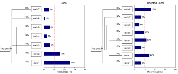
(a) meps-20 dataset.

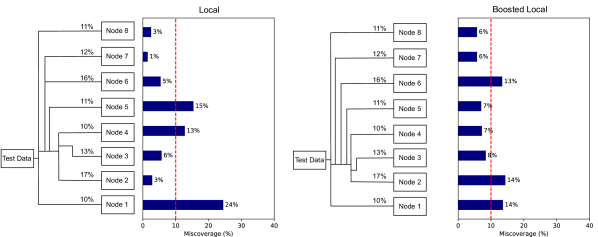
(b) meps-21 dataset.

Figure A1: See the caption of Figure 3 for details.

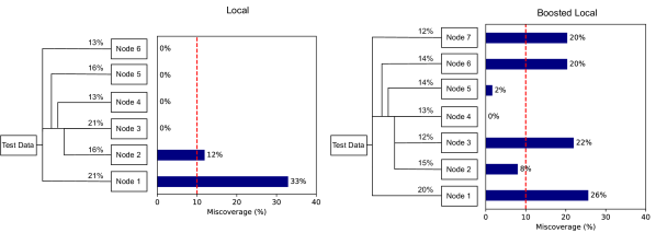
(a) community dataset.

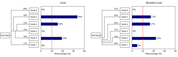
(b) bike dataset.

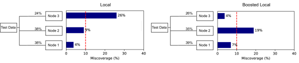
(c) concrete dataset.

Figure A2: See the caption of Figure 3 for details.

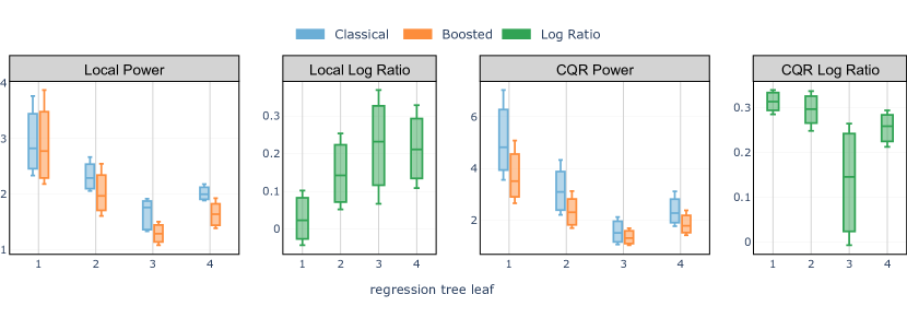
(a) meps-20 dateset.

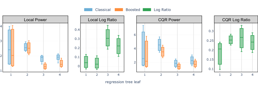
(b) meps-21 dateset.

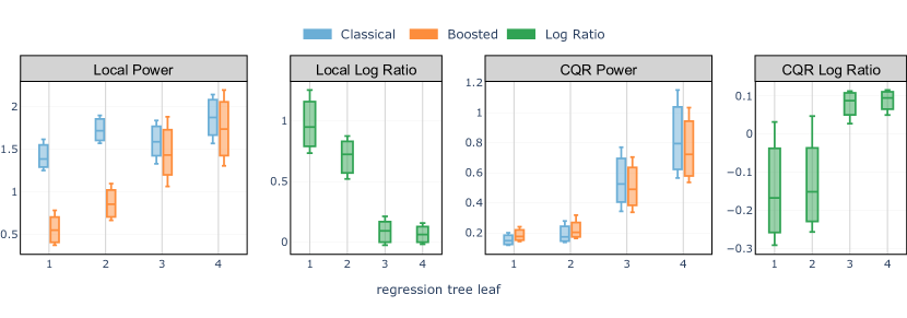
(c) bike dateset.

Figure A3: See the caption of Figure 4 for details.

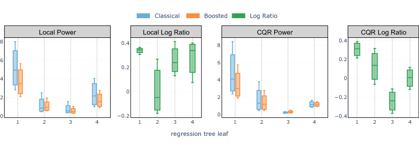
(a) facebook-1 dateset.

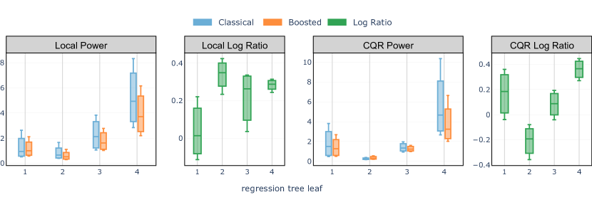
(b) facebook-2 dateset.

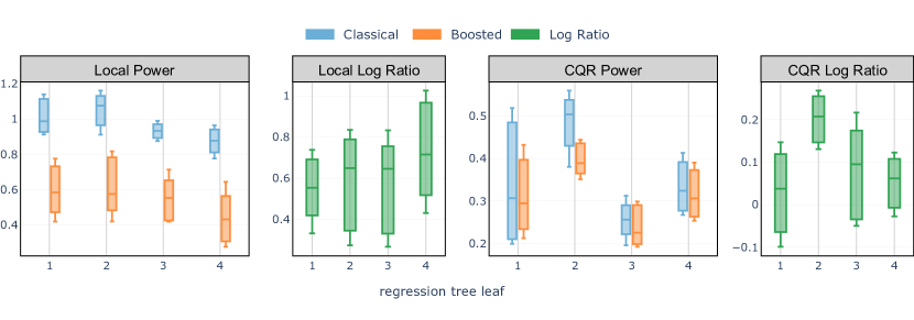
(c) concrete dateset.

Figure A4: See the caption of Figure 4 for details.

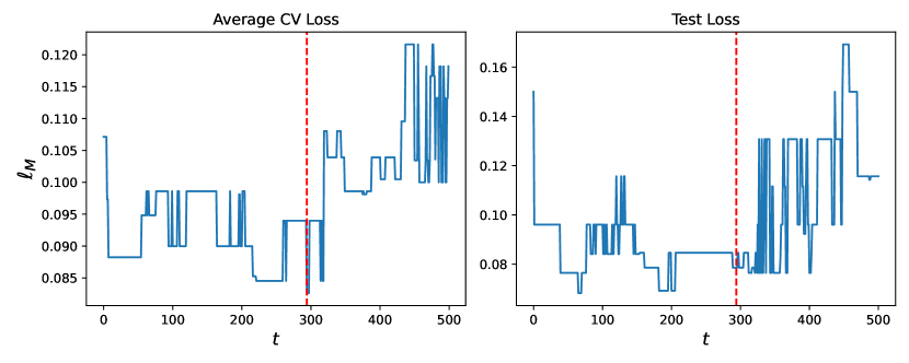
(a) seed 9.

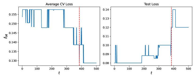
(b) seed 8.

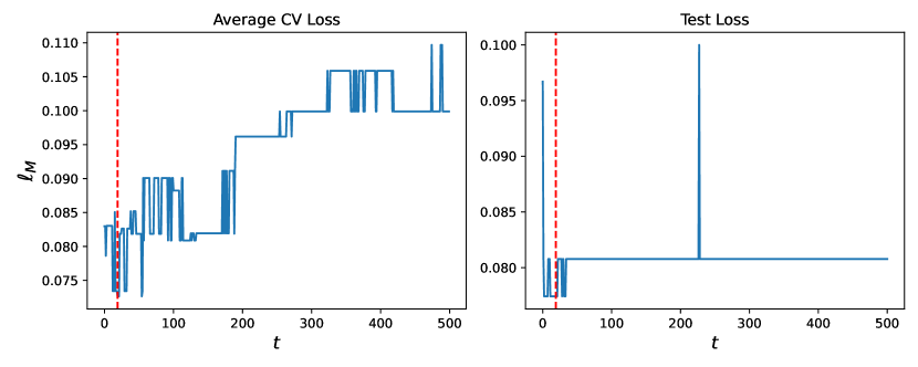
(c) seed 7.

Figure A5: Empirical maximum deviation $\ell_{M}$ across $T=500$ boosting rounds evaluated on dataset concrete under random seeds 7, 8, 9, train-calibration ratio $60\%$ : The left panel illustrates the cross-validated loss, computed as the average across $k=3$ sub-calibration folds. The right panel displays the test loss. The optimal number of boosting rounds $\tau$, determined through cross-validation as specified in (11), is highlighted in red.

References

- [1] Frank E. Harrell and C.. Davis “A New Distribution-Free Quantile Estimator” In Biometrika 69.3 [Oxford University Press, Biometrika Trust], 1982, pp. 635–640 URL: http://www.jstor.org/stable/2335999
- [2] Stephen P Boyd and Lieven Vandenberghe “Convex optimization” Cambridge university press, 2004
- [3] “Classification with conformal predictors” In Algorithmic Learning in a Random World Boston, MA: Springer US, 2005, pp. 53–96 DOI: 10.1007/0-387-25061-1˙3
- [4] Vladimir Vovk, Alexander Gammerman and Glenn Shafer “Algorithmic learning in a random world” Springer, 2005
- [5] I-Cheng Yeh “Concrete Compressive Strength” DOI: https://doi.org/10.24432/C5PK67, UCI Machine Learning Repository, 2007
- [6] C.M. Achilles et al. “Tennessee’s student teacher achievement ratio (STAR) project”, 2008
- [7] Michael Redmond “Communities and Crime” DOI: https://doi.org/10.24432/C53W3X, UCI Machine Learning Repository, 2009
- [8] Vladimir Vovk “Conditional validity of inductive conformal predictors” In Asian conference on machine learning, 2012, pp. 475–490 PMLR
- [9] Hadi Fanaee-T “Bike Sharing Dataset” DOI: https://doi.org/10.24432/C5W894, UCI Machine Learning Repository, 2013
- [10] Prashant Rana “Physicochemical Properties of Protein Tertiary Structure” DOI: https://doi.org/10.24432/C5QW3H, UCI Machine Learning Repository, 2013
- [11] Krisztian Buza “BlogFeedback” DOI: https://doi.org/10.24432/C58S3F, UCI Machine Learning Repository, 2014
- [12] Tianqi Chen and Carlos Guestrin “Xgboost: A scalable tree boosting system” In Proceedings of the 22nd acm sigkdd international conference on knowledge discovery and data mining, 2016, pp. 785–794
- [13] Kamaljot Singh “Facebook Comment Volume Dataset” DOI: https://doi.org/10.24432/C5Q886, UCI Machine Learning Repository, 2016
- [14] Andre Esteva et al. “Dermatologist-level classification of skin cancer with deep neural networks” In nature 542.7639 Nature Publishing Group, 2017, pp. 115–118
- [15] Guolin Ke et al. “Lightgbm: A highly efficient gradient boosting decision tree” In Advances in neural information processing systems 30, 2017
- [16] Jing Lei et al. “Distribution-Free Predictive Inference for Regression” In Journal of the American Statistical Association 113.523 Taylor & Francis, 2018, pp. 1094–1111 DOI: 10.1080/01621459.2017.1307116
- [17] Yaniv Romano, Evan Patterson and Emmanuel Candes “Conformalized quantile regression” In Advances in neural information processing systems 32, 2019
- [18] Yaniv Romano, Evan Patterson and Emmanuel J. Candès “Conformalized Quantile Regression” In Proceedings of the 33rd International Conference on Neural Information Processing Systems Red Hook, NY, USA: Curran Associates Inc., 2019
- [19] Mathieu Blondel, Olivier Teboul, Quentin Berthet and Josip Djolonga “Fast differentiable sorting and ranking” In International Conference on Machine Learning, 2020, pp. 950–959 PMLR
- [20] Rina Foygel Barber, Emmanuel J Candès, Aaditya Ramdas and Ryan J Tibshirani “The limits of distribution-free conditional predictive inference” In Information and Inference: A Journal of the IMA 10.2, 2020, pp. 455–482 DOI: 10.1093/imaiai/iaaa017
- [21] Jerome H. Friedman “Contrast trees and distribution boosting” In Proceedings of the National Academy of Sciences 117.35, 2020, pp. 21175–21184 DOI: 10.1073/pnas.1921562117
- [22] Danijel Kivaranovic, Kory D. Johnson and Hannes Leeb “Adaptive, Distribution-Free Prediction Intervals for Deep Networks”, 2020 arXiv:1905.10634 [stat.ML]
- [23] Matteo Sesia and Emmanuel J Candès “A comparison of some conformal quantile regression methods” In Stat 9.1 Wiley Online Library, 2020, pp. e261
- [24] John Jumper et al. “Highly accurate protein structure prediction with AlphaFold” In Nature 596.7873 Nature Publishing Group, 2021, pp. 583–589
- [25] Kuang-Ting Ko et al. “Structure of the malaria vaccine candidate Pfs48/45 and its recognition by transmission blocking antibodies” In Nature Communications 13.1 Nature Publishing Group UK London, 2022, pp. 5603
- [26] David Stutz, Krishnamurthy Dj Dvijotham, Ali Taylan Cemgil and Arnaud Doucet “Learning Optimal Conformal Classifiers” In International Conference on Learning Representations, 2022 URL: https://openreview.net/forum?id=t8O-4LKFVx
- [27] Isaac Gibbs, John J. Cherian and Emmanuel J. Candès “Conformal Prediction With Conditional Guarantees”, 2023 arXiv:2305.12616 [stat.ME]
- [28] Kexin Huang, Ying Jin, Emmanuel Candès and Jure Leskovec “Uncertainty Quantification over Graph with Conformalized Graph Neural Networks”, 2023 arXiv:2305.14535 [cs.LG]
- [29] “Medical expenditure panel survey, panel 19” URL: https://meps.ahrq.gov/mepsweb/data_stats/download_data_files_detail.jsp?cboPufNumber=HC-181
- [30] “Medical expenditure panel survey, panel 20” URL: https://meps.ahrq.gov/mepsweb/data_stats/download_data_files_detail.jsp?cboPufNumber=HC-181
- [31] “Medical expenditure panel survey, panel 21” URL: https://meps.ahrq.gov/mepsweb/data_stats/download_data_files_detail.jsp?cboPufNumber=HC-192