Accuracy and limitations of the bond polarizability model in modeling of Raman scattering from molecular dynamics simulations

Abstract

Calculation of Raman scattering from molecular dynamics (MD) simulations requires accurate modeling of the evolution of the electronic polarizability of the system along its MD trajectory. For large systems, this necessitates the use of atomistic models to represent the dependence of electronic polarizability on atomic coordinates. The bond polarizability model (BPM) is the simplest such model and has been used for modeling the Raman spectra of molecular systems but has not been applied to solid-state systems. Here, we systematically investigate the accuracy and limitations of the BPM parameterized from density functional theory (DFT) results for a series of simple molecules such as CO₂, SO₂, H₂S, H₂O, NH₃, and CH₄, the more complex CH₂O, CH₃OH and CH₃CH₂OH and thiophene molecules and the BaTiO₃ and CsPbBr₃ perovskite solids. We find that BPM can reliably reproduce the overall features of the Raman spectra such as shifts of peak positions. However, with the exception of highly symmetric systems, the assumption of non-interacting bonds limits the quantitative accuracy of the BPM; this assumption also leads to qualitatively inaccurate polarizability evolution and Raman spectra for systems where large deviations from the ground state structure are present.

I INTRODUCTION

Spectroscopy is as a powerful tool that has been widely applied to various inorganic and organic systems to obtain the characteristic vibrations and other related properties Orlando et al. (2021); Long (2002). The application of molecular dynamics (MD) simulations for the interpretation of infrared (IR) spectra has provided a powerful method for detailed understanding of experimental IR spectroscopy results, significantly enhancing the value provided by IR spectra Gastegger et al. (2017); Gaigeot and Sprik (2003). By contrast, obtaining a similar level of microscopic insight from Raman scattering with the help of MD simulations has not been possible due to the difficulties in the evaluation of the electronic polarizability trajectory.

The Raman spectrum of a system owing to its lattice dynamics can be calculated from the changes in the electronic polarizability of the system due to its atomic (or ionic) vibrations. Therefore, to model the Raman spectra using MD simulations, electronic polarizability along the trajectory of the system dynamics must be calculated, and then the Raman spectrum can be obtained from the auto-correlation function of the time-dependent electronic polarizability trajectory Thomas et al. (2013); Putrino and Parrinello (2002); Luber et al. (2014). Electronic polarizability is an observable related to the electronic response of the system to the perturbation by an applied electric field, and ideally should be obtained by quantum-mechanical (QM) calculations Mattiat and Luber (2021); Lazzeri and Mauri (2003). However, such QM calculation of electronic polarizability at each time step has a very high computational cost. While atomistic models using neural networks for estimation of electronic polarizability trajectories have been developed, due to their complexity they still have a high computational cost, albeit much smaller one than that of direct QM calculations, and require large amount of QM data for model training Lussier et al. (2020); Sommers et al. (2020); Berger et al. (2024); Raimbault et al. (2019). Therefore, modeling the electronic polarizability dynamics for large systems is still challenging.

Among the atomistic approaches for electronic polarizability evaluation, the bond polarizability model (BPM) Montero and del Rio (1976); Cardona et al. ; 199 (1996), is the simplest and the most computationally efficient. This simple model is based on the assumption that the total polarizability of the system is the sum of the polarizability contributions of the individual bonds. The model also assumes that the polarizability contribution of each bond is a function of the length of that bond only, i.e. independent bond approximation. Despite these simplistic assumptions, BPM has been applied and found to be accurate for obtaining Raman spectra in various systems Liang et al. (2017); Wirtz et al. (2005); Luo et al. (2015); Umari et al. (2001). However, it was also found to be inaccurate for some molecular and solid state systems Hermet et al. (2006); Berger and Komsa (2023). Therefore, it is important to analyze the BPM as the simplest possible electronic polarizability model to systematically evaluate the limits of its applicability to the study of molecular and solid-state systems and to provide a baseline reference for the development of more sophisticated electronic polarizablity models.

In this paper, we first applied the BPM to simple molecules such as the linear molecule CO₂, and several two-element non-linear molecules SO₂, H₂S, H₂O, NH₃ and CH₄ with different bond angles; these molecules are used as model systems to understand the effect of bond angles on the BPM accuracy. We then examined the more complicated multielement CH₂O and CH₃OH and CH₃CH₂OH and thiophene molecules to understand the impact of various degrees of freedom of molecular structures on larger molecules in the application of BPM. Finally, we applied the BPM to perovskites as model solid state systems due to their broad range of functional properties and rich physics. In particular, we focused on the classic oxide ferroelectric (FE) BaTiO₃ (BTO) and halide perovskite CsPbBr₃ (CPB). For all of these systems, we compare the BPM results for the polarizability and Raman spectra with those obtained by direct density functional theory (DFT) calculations for small systems. Our results show that despite its simplicity, BPM can be useful and accurate for capturing the overall features of the Raman spectra; however, BPM fails to reproduce fine polarizability changes and some features of Raman spectra when encountering strong asymmetric vibrations and strong anharmonicity. Our results thus demonstrate the limits of accuracy of the BPM approach, providing guidance for modeling of Raman spectroscopy results and also providing a baseline for the development of more accurate atomistic and neural network models of polarizability dynamics.

II Methods

II.1 Bond Polarizability Model and computational methods

In this work, the total polarizability tensor ($\alpha_{ij}$) is defined as

$$\alpha_{ij}=\frac{1}{\Omega}\sum_{n}\alpha_{ij}^{n}$$

where $\Omega$ is the volume and $\alpha_{ij}^{n}$ is the polarizability tensor for the $n^{th}$ bond. Furthermore, $\alpha_{ij}^{n}$ is defined as

$$\alpha_{ij}^{n}=\frac{1}{3}(\alpha_{l}+2\alpha_{p})\delta_{ij}+(\alpha_{l}-\alpha_{p})(\frac{R_{i}R_{j}}{R^{2}}-\frac{1}{3}\delta_{ij})$$

where $i$, $j$ denote $x$, $y$ or $z$ axes. $R$ is the vector between two atoms forming the $n^{th}$ bond, and $\alpha_{l}$ and $\alpha_{p}$ are the longitudinal and perpendicular bond polarizabilities, respectively for a particular bond type. According to BPM, these parameters are functions of the bond length $R$ only. Therefore, the bond polarizabilities can be expanded in a Taylor series with respect to the bond length around the equilibrium structure denoted by superscript 0, as given by

$$\alpha_{t}=\alpha_{t}^{0}+\alpha_{t}^{1}.(R-R^{0})+\alpha_{t}^{2}.(R-R^{0})^{2}+..$$

where $\alpha_{t}$ is either longitudinal ($t$ = $l$) or perpendicular ($t$ = $p$) component of the bond polarizability.

In order to extract the unknown parameters of the BPM, we calculated polarizability trajectory using density functional perturbation theory (DFPT) Baroni et al. (2001) as implemented in Quantum ESPRESSO code Giannozzi et al. (2009). For all of the systems considered here, $ab$ $initio$ molecular dynamics were also performed using Quantum ESPRESSO. The Perdew-Burke-Ernzerhof exchange-correlation functional for solids (PBEsol) was employed for all systems Perdew et al. (2008). All the unknown parameters in the BPM then were extracted by minimizing the difference between the model results and the training data set along the DFPT-calculated polarizability trajectory.

For CO₂, SO₂, H₂S, H₂O and NH₃, $ab$ $initio$ molecular dynamics simulations were performed at 300 K. First, we calculated polarizability trajectory directly using DFT for 30, 24, 24, 25 and 24 ps with a time step of 0.0015 ps for the CO₂, SO₂, H₂S, H₂O and NH₃ molecules, respectively. However, due to computational cost, we considered the DFT-calculated polarizability trajectory for 23, 24, 23, 20 and 20 ps with a time step of 0.0058, 0.0058, 0.0058, 0.0072 and 0.0072 ps in case of CH₄, CH₂O, CH₃OH, CH₃CH₂OH and thiophene, respectively. We then extracted the BPM parameters for 1^st- and 2^nd-order models using the DFT-calculated polarizability trajectory data.

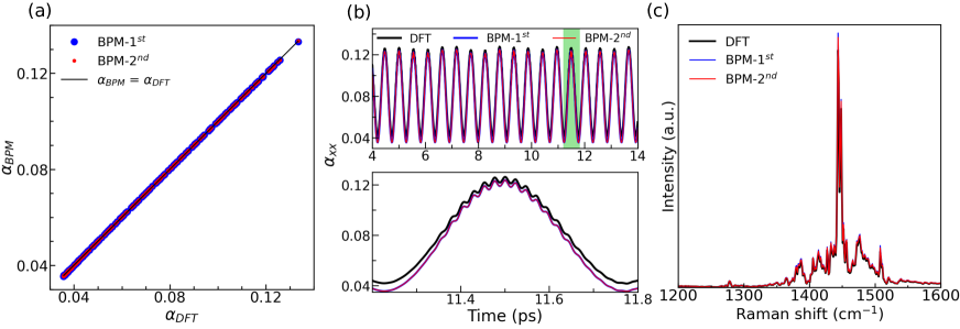
Figure 1: (Color online) CO₂: (a) The $xx$ component of $\alpha_{BPM}$ (1^st and 2^nd order are shown by blue and red circles, respectively) vs $\alpha_{DFT}$. The linear fit of BPM-2^nd order data is shown by the black line.. (b) Top panel: Comparison of time-dependent trajectory of $\alpha_{xx}$. Bottom panel: Magnified view of the region in first panel marked in filled green color. (c) Raman spectra from DFT (black), BPM-1^st (blue) and BPM-2^nd (red).

For BTO and CPB, we found that the polarizability is dominated by the contributions from the motions of the TiO₆ and PbBr₆ octahedra (see Supplementary Material (SM)). Therefore, BPM parameters are extracted after fitting to the Ti-O and Pb-Br bonds, respectively, for these systems. We considered a 10-atom unit cell and performed molecular dynamics for 30 ps with a time step of 0.0015 ps while keeping the cell volume fixed at four temperatures of 300 K, 600 K, 800 K and 1000 K, respectively. For the DFT-calculated polarizability trajectory, we considered the full trajectory of 30 ps with a time step of 0.073 ps. The DFT-calculated polarizability trajectories for all temperatures were used for the extraction of the BPM parameters.

For classical molecular dynamics of BTO, we used a 10$\times$10$\times$10 supercell for 300 ps with a time step of 0.001 ps with the LAMMPS code Thompson et al. (2022) using the bond-valence model atomistic potential (BVMD) Qi et al. (2016). Then, BPM parameters as extracted from the polarizability calculations for the 10-atom unit cell were used to calculate the Raman spectra of bulk and thin film of BTO for various temperatures.

II.2 Experimental details

Raman scattering was collected in the backscattering configuration ($Z(X,X)\bar{Z}$, X$\parallel$(100)), with a 5 mW 385 nm laser excitation source focused to a surface intensity of 1 W/cm². Light was dispersed by a triple spectrometer operated in a double-dispersive single-subtractive mode (Horiba Jobin-Yvon, model T64000), and collected using a thermoelectrically-cooled CCD (Andor). The (001)-oriented BaTiO₃ bulk single crystal was grown by top seeded solution growth (MTI Corp.).

Raman spectra were collected between 123 K and 423 K at 5 K intervals, and each individual spectrum is the average of 3 acquisitions for 10 s each. Experimental observations of abrupt structural phase transitions at 183 K (rhombohedral (R) to orthorhombic (O)), 278 K (O to tetragonal (T)), and 393 K (T to cubic (C)) are in agreement with the BTO results reported in the literatureDeluca et al. (2018). Additionally, the intensity of the collapsing soft mode (160 cm^-1 in the R-phase, and the broad feature at 35 cm^-1 in the O-phase) are an indication of structural homogeneity and a low population of domain walls, showing that these are effectively single-domain measurementsYuzyuk (2012).

III RESULTS AND DISCUSSION

III.1 Linear CO₂ molecule

Fig. 1 (a) compares the polarizabilities calculated using BPM and DFT along the polarizability trajectory of the $xx$ component at 300 K for CO₂. Both 1^st- and 2^nd-order BPM reproduce the DFT polarizability very accurately (see the linear fit of the 2^nd order BPM data). We also compare polarizability trajectory ($\alpha_{xx}$) as calculated from DFT and BPM (1^st and 2^nd) in Fig. 1 (b). The top panel of Fig. 1 (b), which presents the overall polarizability trajectory, shows perfect agreement between the overall trajectories from BPM and DFT, corresponding to low-frequency vibrations. The bottom panel of Fig. 1 (b), which presents a magnified view of a small region of the trajectory also shows good agreement between the model and DFT results for the high-frequency polarizability oscillations. This demonstrates the accuracy of BPM on simple linear molecule such as CO₂. Therefore, it is expected that the Raman spectrum calculated using BPM will capture the main peaks of the DFT Raman spectrum. Fig. 1 (c) shows the perfect overlap of peak positions and intensities of the Raman spectra obtained by these two methods. These results show that the polarizability fluctuations are well-reproduced by the BPM.

III.2 Nonlinear molecules

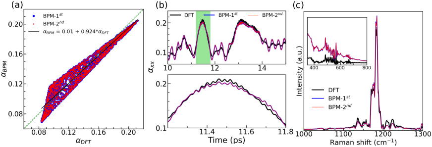
Figure 2: (Color online) SO₂ (a) The $xx$ component of $\alpha_{BPM}$ (1^st and 2^nd order are shown by blue and red circles, respectively) vs $\alpha_{DFT}$. The linear fit of the BPM-2^nd order data is shown by solid black line. The green dotted line represents $\alpha_{BPM}$ = $\alpha_{DFT}$. (b) Top panel: Comparison of the trajectory of $\alpha_{xx}$. Bottom panel: Magnified view of the region shaded in green in the first panel. (c) Raman spectra from DFT (black), BPM-1^st (blue) and BPM-2^nd (red) results. Inset shows the results in the lower-wavenumber region.

Then, we considered the SO₂, H₂S, H₂O, NH₃ and CH₄ nonlinear molecules in order to examine the effect of angular geometry on the BPM accuracy. Fig. 2 (a) compares the calculated values of the the $xx$ component of $\alpha_{BPM}$ for 1^st and 2^nd order BPM with $\alpha_{DFT}$ for SO₂. The scatter of the data around the $y$ = $x$ line ($\alpha_{BPM}$ = $\alpha_{DFT}$) shows that the 1^st-order BPM cannot fully capture the DFT values. These results are not improved even after the application of the 2^nd-order BPM. However, an overall linear dependence of $\alpha_{BPM}$ plotted versus $\alpha_{DFT}$ is observed (the equation of the linear fit of the 2^nd order BPM $\alpha$ values plotted versus DFT $\alpha$ values is $\alpha_{BPM}$ = 0.01 + 0.924*$\alpha_{DFT}$) with an increase of the deviation of the value of $\alpha_{BPM}$ from $\alpha_{DFT}$ when going from larger to smaller values of $\alpha_{DFT}$, forming a triangular-like data distribution. We also plotted the polarizability trajectories at 300 K of SO₂ from these different methods in Fig. 2 (b). The gross features of the DFT trajectory are reproduced well by the 1^st and 2^nd order BPM. Even though the low-frequency (top panel of Fig. 2 (b)) and high-frequency (bottom panel of Fig. 2 (b)) polarizability fluctuations are well-captured by the BPM, the amplitude of the low- and high-frequency fluctuations from the BPM results shows some differences from the DFT results. These discrepancies are reflected in the calculated Raman spectra for the high-frequency region (see Fig. 2 (c)), where the spectral positions of the DFT-generated spectra are reproduced well by the BPM-generated spectra. However, unlike for CO₂, the peak intensities from BPM do not agree with the DFT results. Additionally, differences between the Raman intensities of the DFT and BPM spectra are also observed for the low-frequency peaks (see inset Fig. 2 (c)).

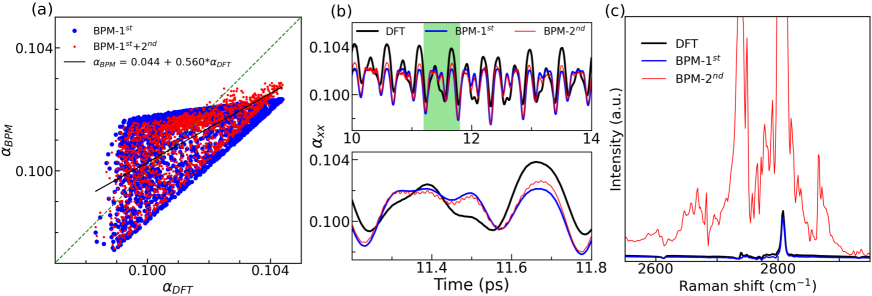
Figure 3: (Color online) H₂S: (Color online) (a) The results for the $xx$ component of $\alpha_{BPM}$ (1^st and 2^nd order BPM are shown by blue and red circles, respectively) plotted vs $\alpha_{DFT}$. The linear fit of BPM-2^nd order data is shown by the black line. The green dotted line represents $\alpha_{BPM}$ = $\alpha_{DFT}$. (b) Top panel: Comparison of the trajectory of $\alpha_{xx}$. Bottom panel: Magnified view of the region in the first panel shaded in green. (c) Raman spectra generated using DFT (black), BPM-1^st (blue) and BPM-2^nd (red).

Next, we examined the BPM results for H₂S. Fig. 3 (a), presents the results for BPM-calculated $\alpha$ plotted versus DFT-calculated $\alpha$ for the $xx$ component. Similar to SO₂, the 1^st order $\alpha_{BPM}$ values show high scatter in comparison to $\alpha_{DFT}$ forming a triangular data distribution where the deviation of the BPM-generated $\alpha$ values from the DFT-generated $\alpha$ increases drastically while moving from higher to lower values of DFT-generated $\alpha$. Inclusion of 2^nd order in the BPM improves the results slightly so that only a small decrease in the size of the triangular data distribution is obtained. The inclusion of higher-order (3^rd and 4^th order) terms in the BPM did not eliminate this error, indicating that it is due to the lack of consideration of the effects of the H-S-H angle on the polarizability. The $\alpha_{xx}$ polarizability trajectories from different methods are shown in Fig. 3 (b), revealing poor agreement between the BPM- and DFT-calculated polarizability trajectories. A small improvement by the 2^nd-order model compared to the 1^st-order model is observed for the overall variation of $\alpha_{xx}$ (Top panel of Fig. 3 (b)). However, a magnified view of the $\alpha_{xx}$ trajectories shows that the 2^nd-order model trajectory exhibits much stronger high-frequency fluctuations compared to both the DFT or 1^st-order model trajectories.

These much stronger high-frequency fluctuations lead to a dramatically higher Raman intensity for the high-frequency peaks predicted by the 2^nd-order model compared to the DFT and 1^st order model spectra (Fig. 3 (c)). Both BPM-1^st and BPM-2^nd order models predict peak positions similar to those of DFT in the high-frequency spectrum. However, comparison of the obtained peak intensities shows that the BPM-1^st spectrum is closer to the DFT spectrum than the BPM-2^nd spectrum. The unphysicallly high intensity of the high-frequency fluctuations in the BPM-2^nd order model is likely due to the fact that the model parameterization procedure seeks to minimize the overall error; since the high-frequency oscillations are much weaker than the low-frequency oscillations, an overestimation of high-frequency amplitude will be acceptable in the parameterization if it is balanced by better agreement with the overall trajectory. However, this will lead to unphysically high intensity in the physically relevant part of the spectrum.

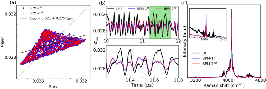
Figure 4: (Color online) H₂O: (Color online) (a) The results for the $xx$ component of $\alpha_{BPM}$ (1^st and 2^nd order BPM are shown by blue and red circles, respectively) plotted vs $\alpha_{DFT}$. The linear fit of BPM-2^nd order data is shown by the black line. The green dotted line represents $\alpha_{BPM}$ = $\alpha_{DFT}$. (b) Top panel: Comparison of the trajectory of $\alpha_{xx}$. Bottom panel: Magnified view of the region in the first panel shaded in green. (c) Raman spectra generated using DFT (black), BPM-1^st (blue) and BPM-2^nd (red).

We then examine the performance of BPM for H₂O, perhaps the most important molecule in chemistry and biology. Fig. 4 (a) shows $\alpha_{xx}$ calculated using BPM-1^st and BPM-2^nd for different H₂O geometries plotted versus the corresponding DFT $\alpha_{xx}$ values. Similar to other nonlinear molecules, a triangular data distribution is observed for both BPM-1^st and BPM-2^nd. However, unlike for H₂S, the inclusion of 2^nd order does not improve the BPM results. The calculated slope (0.275) of the linear fit of the BPM-2^nd vs DFT data is even worse than that for H₂S (0.560). We also plot the polarizability trajectories as calculated from BPM-1^st, BPM-2^nd and DFT methods in Fig. 4 (b). The low-frequency polarizability trajectory (see top panel of Fig. 4 (b)) is not well-captured by BPM. However, the high-frequency oscillations of the polarizability trajectory are well-reproduced by BPM (see bottom panel of Fig. 4 (b)). This implies that the BPM-calculated Raman spectrum will be in good agreement with the DFT spectrum in the high-frequency region but not in the low-frequency region. The Raman spectra (Fig. 4 (c)) calculated from the polarizability trajectory show that the peak position in the high-frequency range is well-reproduced by the BPM-1^st and BPM-2^nd. However, a small disagreement between the peak intensities between BPM and DFT spectra is observed in this region. By contrast, the spectra in the low-frequency region (inset of Fig. 4 (c)) do not show good agreement with the DFT results.

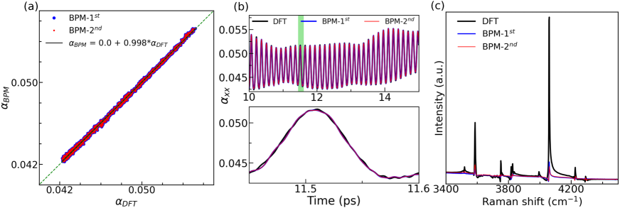
Figure 5: (Color online) NH₃: (Color online) (a) The results for the $xx$ component of $\alpha_{BPM}$ (1^st and 2^nd order BPM are shown by blue and red circles, respectively) plotted vs $\alpha_{DFT}$. The linear fit of BPM-2^nd order data is shown by the black line. The green dotted line represents $\alpha_{BPM}$ = $\alpha_{DFT}$. (b) Top panel: Comparison of the trajectory of $\alpha_{xx}$. Bottom Panel: Magnified view of the region in the top panel shaded in green. (c) Raman spectra generated using DFT (black), BPM-1^st (blue) and BPM-2^nd (red).

Next, we consider NH₃ and CH₄ which are nonlinear molecules with multiple equal bond angles. While naively, one may expect the BPM polarizability to show stronger disagreement with DFT results for NH₃ compared to H₂O due to a greater number of bond angles, in contrast to the results for H₂S, H₂O and SO₂, the plot of BPM polarizability versus DFT polarizability shows a good linear trend Fig. 5 (a). The overall $\alpha_{xx}$ trajectory is also reproduced well (top panel of Fig. 5 (b)). However, a magnified view of the trajectory shows significant differences between the high-frequency $\alpha_{xx}$ oscillations predicted by BPM and those obtained by DFT calculations, with much larger amplitude of oscillations for the DFT trajectory (bottom panel of Fig. 5 (b)). Correspondingly, examination of the Raman spectra presented in Fig. 5 (c) shows that the high-frequency peaks of the DFT spectrum have much higher intensity than the corresponding BPM peaks. While BPM and DFT obtain the same frequencies for the peaks, the relative intensities of the peaks are somewhat different. Thus, similar to H₂S, H₂O and SO₂, BPM correctly reproduces the peak positions but does not accurately reproduce the fine features of the DFT spectra.

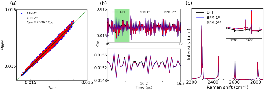
Figure 6: (Color online) CH₄: (Color online) (a) The results for the $xx$ component of $\alpha_{BPM}$ (1^st and 2^nd order BPM are shown by blue and red circles, respectively) plotted vs $\alpha_{DFT}$. The linear fit of BPM-2^nd order data is shown by the black line. The green dotted line represents $\alpha_{BPM}$ = $\alpha_{DFT}$. (b) Top panel: Comparison of the trajectory of $\alpha_{xx}$. Bottom panel: Magnified view of the region in the first panel shaded in green. (c) Raman spectra generated using DFT (black), BPM-1^st (blue) and BPM-2^nd (red).

Next, examination of the CH₄ results in Fig. 6 reveals good agreement between BPM and DFT results with only a small deviation from $y$ = $x$ line. A close examination of the polarizability trajectory and the Raman spectrum reveals small but noticeable differences. Thus, while accurate, the BPM for CH₄ does not show perfect agreement such as that found for CO₂, indicating that the lack of a bond-angle-dependent term in the BPM does affect the accuracy of model polarizability, even though the effect is weak.

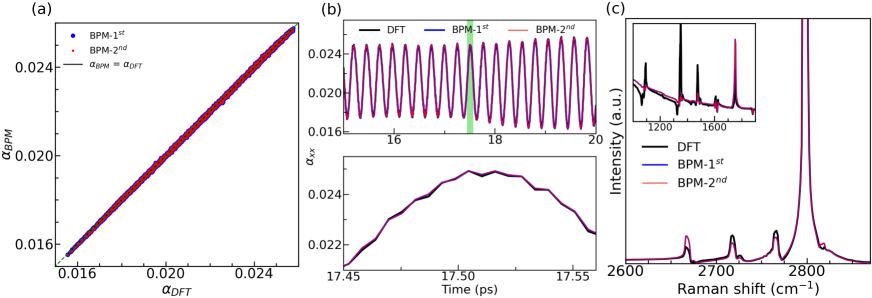
Figure 7: (Color online) CH₂O: (Color online) (a) The results for the $xx$ component of $\alpha_{BPM}$ (1^st and 2^nd order BPM are shown by blue and red circles, respectively) plotted vs $\alpha_{DFT}$. The linear fit of BPM-2^nd order data is shown by the black line. The green dotted line represents $\alpha_{BPM}$ = $\alpha_{DFT}$. (b) Top panel: Comparison of the trajectory of $\alpha_{xx}$. Bottom panel: Magnified view of the region in the first panel shaded in green. (c) Raman spectra generated using DFT (black), BPM-1^st (blue) and BPM-2^nd (red).

We now discuss the origin of the polarizability errors of the BPM in the angular molecules. The BPM is a Taylor expansion of the polarizability around the ground state structure, where rather than carrying out the Taylor expansion in terms of the Cartesian coordinates of the atoms, the Taylor expansion is carried out in terms of the deviations of the bond lengths from their ground state values. However, for tri-atomic molecules, in addition to the bond lengths, the bond angle can also affect the polarizability and a full Taylor expansion should involve angle-dependent terms such a $a_{\theta}\Delta\theta$ + $b_{\theta}(\Delta\theta)^{2}$ +.. as well as cross-terms describing the interplay of the effects of the bond length and bond angle, such as $a_{r,\theta}\Delta\theta\Delta r$ + … . Clearly, these terms are absent in the BPM that only takes into account the changes in the bond lengths and ignores the effect of the angle.

For a Taylor expansion, we expect that higher-order terms are weaker than the lower-order terms. Thus, the linear effect of the change in $\theta$ given by $a_{\theta}\Delta\theta$ is larger than the quadratic effect given by $b_{\theta}(\Delta\theta)^{2}$. In a tri-atomic angular molecule such as water, a vibration that changes the bond angle will change the polarizability by $a_{\theta}\Delta\theta$ + $b_{\theta}\Delta\theta^{2}$ + $a_{r,\theta}\Delta\theta\Delta r$. For the water molecule with only one bond angle, any motion of the O-H bonds that changes the bond angle is uncompensated by an equal and opposite change in a different bond angle, so that the error is of the order $a_{\theta}\Delta\theta$ + $b_{\theta}(\Delta\theta)^{2}$ + $a_{r,\theta}\Delta\theta\Delta r$. However, for a molecule such as CH₄, any movement of the C-H bond that leads to a change in the bond angle makes one bond angle smaller and another bond angle greater. This leads to the cancellation of the first-order effects of both the $\theta$ and the $\theta r$ terms, so that the error is given by $b_{\theta}(\Delta\theta)^{2}$ only and is much smaller than that for water. For NH₃, the size of the error depends on the direction of vibration. For a vibration by an N-H bond toward another N-H bonds, the linear effects will be canceled out and the error due to ignoring the angular effect will be only second order in $\Delta\theta$ and small. However for a vibration by an N-H bond toward the N lone pair, the linear angular effect will be present and the error will be large. Therefore, we observe very larger deviation of BPM results for polarizability in the $\alpha_{BPM}$ vs $\alpha_{DFT}$ plot for angular tri-atomic molecules H₂O, H₂S and SO₂, a much smaller deviation for NH₃ and an even smaller deviation for CH₄.

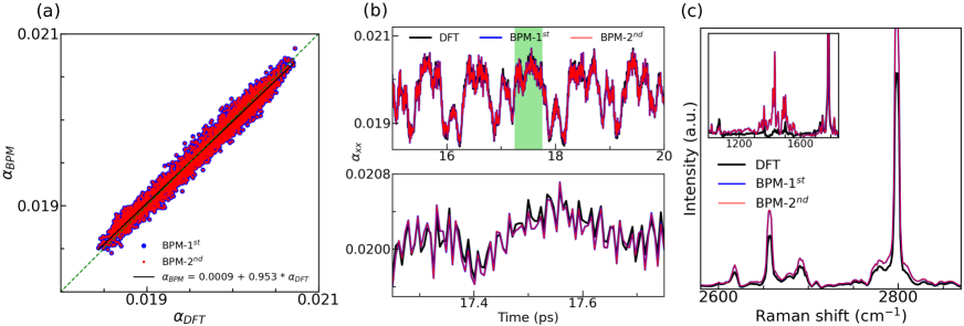
Figure 8: (Color online) CH₃OH: (Color online) (a) The results for the $xx$ component of $\alpha_{BPM}$ (1^st and 2^nd order BPM are shown by blue and red circles, respectively) plotted vs $\alpha_{DFT}$. The linear fit of BPM-2^nd order data is shown by the black line. The green dotted line represents $\alpha_{BPM}$ = $\alpha_{DFT}$. (b) Top panel: Comparison of the trajectory of $\alpha_{xx}$. Bottom panel: Magnified view of the region in the first panel shaded in green. (c) Raman spectra generated using DFT (black), BPM-1^st (blue) and BPM-2^nd (red).

To further test the performance of BPM, we examine the more complicated tri-element molecules CH₂O (see Fig. 7) and CH₃OH (see Fig. 8). We find that despite the strong asymmetry of CH₂O, BMP shows small deviations from the DFT results. This is likely due to the high stiffness of the 120^∘ H-C-O and the H-C-H angles that only allow small vibrations (considerably smaller than those for water) and therefore lead to only small deviations of BPM polarizability from the DFT polarizability even in the presence of error linear in $\theta$. For CH₃OH, we find significant differences between BPM and DFT polarizability values, due to the larger fluctuations of the C-O-H bond angle for which the terms linear in $\theta$ are not canceled out. These results suggest that BPM will be accurate in the case where linear dependence of the polarizability on the bond angle is either zero due to the presence of multiple bonds such that the bond motion makes one bond angle greater and the other bond angle smaller, or is small due to the stiff double bonds. On the other hand, for highly asymmetric molecules with single bonds, and in particular for O atoms where only a single bond angle centered at O is possible, BPM errors due to ignoring the effect of $\theta$ will be significant. Comparison of the BPM results for polarizability and Raman spectra of thiophene (C₄H₄S) and CH₃CH₂OH with the corresponding DFT results confirm the above conclusions. For the aromatic thiophene molecule, small errors are obtained for the BPM polarizability results as shown in Figs. 9, with good agreement obtained for the Raman spectra except for the peak at 1450 cm^-1. This is due to the stiffness of the aromatic structure with 120^∘ bond angles, similar to CH₂O. For CH₃CH₂OH, the agreement between the BPM and DFT polarizability values is similar to that for CH₃OH (see Figs. 10) and the Raman spectrum shows a similar poor agreement with the DFT spectrum for the 1200-1600 cm^-1 region. These results suggest that spectral features related to asymmetric bonds will be reproduced relatively poorly by BPM for large molecule, even while the overall spectrum will show good agreement with DFT results due to the dominance of the functional groups for which the BPM model performs well (e.g. CH₃ and CH₂ in ethanol).

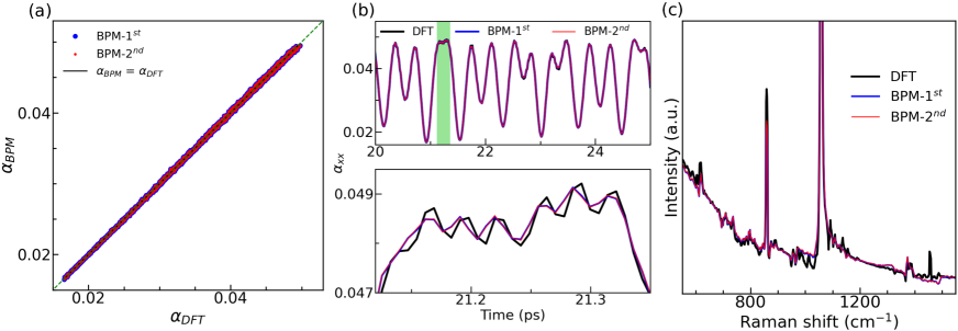
Figure 9: (Color online) Thiophene: (Color online) (a) The results for the $xx$ component of $\alpha_{BPM}$ (1^st and 2^nd order BPM are shown by blue and red circles, respectively) plotted vs $\alpha_{DFT}$. The linear fit of BPM-2^nd order data is shown by the black line. The green dotted line represents $\alpha_{BPM}$ = $\alpha_{DFT}$. (b) Top panel: comparison of the trajectory of $\alpha_{xx}$. Bottom panel: Magnified view of the region in the first panel shaded in green. (c) Raman spectra generated using DFT (black), BPM-1^st (blue) and BPM-2^nd (red).

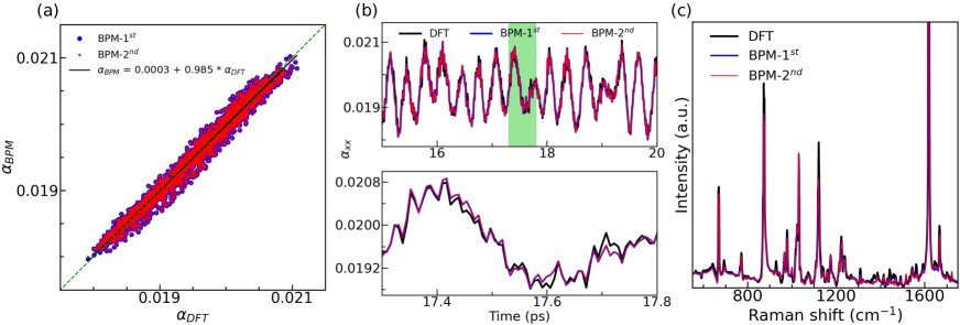
Figure 10: (Color online) CH₃CH₂OH: (Color online) (a) The results for the $xx$ component of $\alpha_{BPM}$ (1^st and 2^nd order BPM are shown by blue and red circles, respectively) plotted vs $\alpha_{DFT}$. The linear fit of BPM-2^nd order data is shown by the black line. The green dotted line represents $\alpha_{BPM}$ = $\alpha_{DFT}$. (b) Top panel: Comparison of the trajectory of $\alpha_{xx}$. Bottom panel: Magnified view of the region in the first panel shaded in green. (c) Raman spectra generated using DFT (black), BPM-1^st (blue) and BPM-2^nd (red).

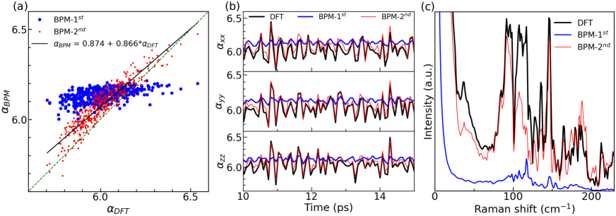
Figure 11: (Color online) BaTiO₃ at 300 K: (Color online) (a) The results for the $xx$ component of $\alpha_{BPM}$ (1^st and 2^nd order BPM are shown by blue and red circles, respectively) plotted vs $\alpha_{DFT}$. The linear fit of BPM-2^nd order data is shown by the black line. The green dotted line represents $\alpha_{BPM}$ = $\alpha_{DFT}$. (b) Comparison of the trajectory of $\alpha_{xx}$ (top panel), $\alpha_{yy}$ (middle panel) and $\alpha_{zz}$ (bottom panel) calculated from DFT (black), BPM-1^st (blue) and BPM-2^nd (red), (c) Raman spectra generated using DFT (black), BPM-1^st (blue) and BPM-2^nd (red).

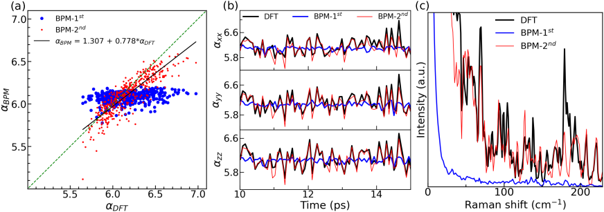
Figure 12: (Color online) BaTiO₃ at 1000 K: (Color online) (a) The results for the $xx$ component of $\alpha_{BPM}$ (1^st and 2^nd order BPM are shown by blue and red circles, respectively) plotted vs $\alpha_{DFT}$. The linear fit of BPM-2^nd order data is shown by the black line. The green dotted line represents $\alpha_{BPM}$ = $\alpha_{DFT}$. (b) Comparison of the trajectory of $\alpha_{xx}$ (top panel), $\alpha_{yy}$ (middle panel) and $\alpha_{zz}$ (bottom panel) calculated from DFT (black), BPM-1^st (blue) and BPM-2^nd (red), (c) Raman spectra generated using DFT (black), BPM-1^st (blue) and BPM-2^nd (red).

III.3 Perovskites

Multicenter bonding is important for solid-state materials and we therefore examine two perovskites, the classic ferroelectric BTO and the CPB halide perovskite, which are representative materials of the important oxide and halide perovskites in order to understand the effectiveness of the BPM for representing solid-state polarizability and Raman spectra. The perovskite structure enables a variety of different distortions that provide a good test of atomistic polarizability models. For example, BTO can assume four different phases generated by different directions of average Ti displacements from the center of the O₆ octahedra that show different Raman spectra. Additionally, the presence of vibrational modes related to O₆ rotations also contributes to the Raman spectra of BTO. The soft bonds and strong distortions of CPB make it a particularly stringent test case for atomistic polarizability models Berger and Komsa (2023).

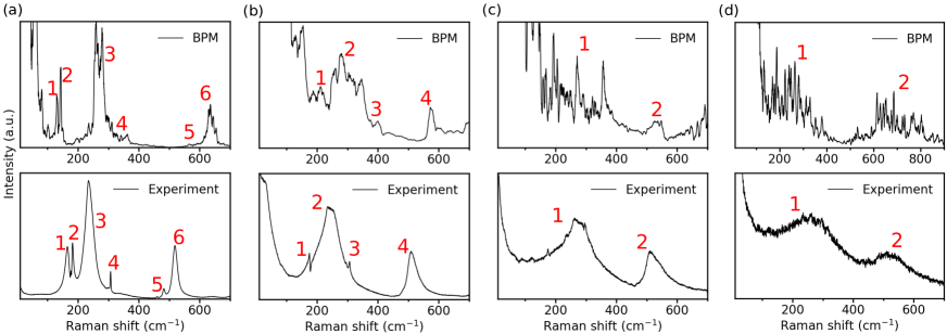
Figure 13: (Color online) Raman spectra of different phases ((a) rhombohedral, (b) orthorhombic), (c) tetragonal, and (d) cubic) of BTO single crystal from bond polarizability model (top panel) and experiment (bottom panel). The temperatures for (a), (b), (c) and (d) are 60 K, 88 K, 110 K and 160 K, respectively (top panel), and 123 K, 233 K, 333 K, 423 K, respectively (bottom panel). Peaks from BPM and experiment are marked by number for comparison.

Fig. 11 (a) plots the $\alpha_{xx}$ values for both 1^st and 2^nd order BPM versus the DFT-calculated polarizability for ten-atom supercell of BTO at 300 K. It is observed that the BPM-1^st order completely fails to reproduce the DFT-calculated polarizability data, whereas the inclusion of 2^nd order term in the BPM strongly improves the model predictions. For example, the slope of the line fit to the BPM-2 data plotted versus DFT data is 0.874, which is relatively close to the $\alpha_{BPM}$ = $\alpha_{DFT}$ straight line. Nevertheless, large scatter is observed in the plot of DFT versus BPM-2^nd polarizability. Inclusion of higher-order dependence of bond polarizability on bond length does not strongly improve the agreement of BPM with DFT (see SM), suggesting that the BPM error is due to the fundamental approximation of independent bond contributions to the polarizability of the BPM.

We then compare the polarizability trajectories ($\alpha_{xx}$, $\alpha_{yy}$, $\alpha_{zz}$) calculated from BPM (1^st and 2^nd) and DFT methods as shown in Fig. 11 (b). The improvement of BPM results can be observed clearly after the inclusion of BPM-2^nd order, which reproduces the overall trajectory well but shows local deviations from the DFT values. Here, we only compare the low-frequency region due to the large time step used to evaluate the polarizability trajectory.

The Raman spectra calculated using the polarizability trajectory with large time steps are shown in Fig. 11 (c). The BPM-2^nd spectrum reproduces all of the peaks of the DFT spectrum, but shows strong differences in intensity for four peaks (at 110, 130, 170 and 215 cm^-1), indicating that BPM-2^nd cannot reliably reproduce the lineshapes of the peaks in the Raman spectrum.

We then applied the same BPM parameters for the structures obtained in the DFT MD simulation of BTO performed at 1000 K in order to check the applicability of the BPM parameters at higher temperatures. Fig. 12 (a) shows the comparison of the BPM-calculated polarizability with the DFT-calculated polarizability. Similar to the 300 K results (Fig. 11 (a)), the BPM-1^st order fail to reproduce the DFT-results. However, the BPM-2^nd improved the value of polarizability so that the data points are more aligned along the $\alpha_{BPM}$ = $\alpha_{DFT}$ straight line. The scatter of the data is greater than that for 300 K, most likely due to the more anharmonic vibrations, greater impact of the changes in the Ti-O-Ti and O-Ti-O bond angles, and greater coupling between the bonds. This can also be seen by comparing the calculated slope from the linear fitting, where the calculated value of the slopes are 0.866 and 0.778 at 300 K and 1000 K, respectively.

The direct comparison of the polarizability trajectories at 1000 K is shown in Fig. 12 (b). Similar to the results for the simulation at 300 K, the BPM-2^nd captures the overall fluctuation of the polarizability very well. These results are also reflected in the calculated Raman spectra plot for the low-frequency region as shown in Fig. 12 (c). Interestingly, despite the stronger deviation of the BPM-2^nd polarizabilities from DFT polarizability for 1000 K than 300 K, the Raman spectrum at 1000 K shows better agreement between DFT and BPM-2^nd with only the peak at 180 cm^-1 showing strong underestimation of the intensity by BPM-2^nd compared to DFT. This is likely either due to error cancellation or because the high errors of BPM-2^nd are relevant for non-Raman-active modes that do not contribute to the error in the Raman spectrum. The lack of reliability of BPM-2^nd for the peak intensity means that the temperature evolution of the Raman peaks is reproduced well for some peaks but is only qualitatively reproduced for other peaks. For example, DFT results for the ten-atom cell dynamics show that the intensity of the peak at 180 cm^-1 is weaker than that at 100 cm^-1 at 300 K and then increases with higher temperature so that at 1000 K the peak at 180 cm^-1 has much higher intensity than the peak at 100 cm^-1. By contrast, BPM-2^nd spectra show that the peak at 180 cm^-1 changes from weaker intensity to same intensity as the peak at 100 cm^-1 when the temperature is changed from 300 to 1000 K. Thus, while the BPM qualitatively reproduces the overall trend of the changes in the relative intensities of the two peaks, it does not provide quantitative agreement with DFT.

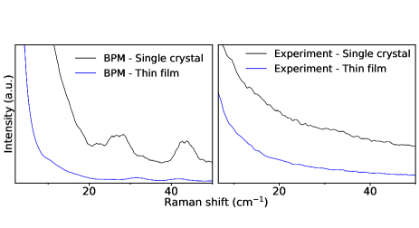
Figure 14: (Color online) Central peak intensity of single crystal (black) and thin film (blue) of BTO (tetragonal phase) from BPM (left panel) and experiment (right panel). The temperature for left panel and right panel are 130 K and 333 K, respectively.

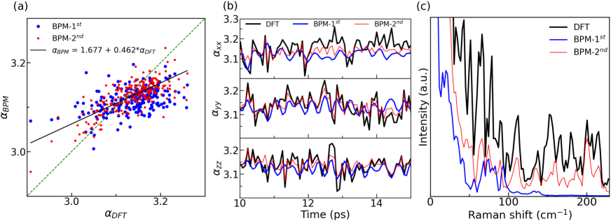
Figure 15: (Color online) CsPbBr₃ at 300 K: (Color online) (a) The results for the $xx$ component of $\alpha_{BPM}$ (1^st and 2^nd order BPM are shown by blue and red circles, respectively) plotted vs $\alpha_{DFT}$. The linear fit of BPM-2^nd order data is shown by the black line. The green dotted line represents $\alpha_{BPM}$ = $\alpha_{DFT}$. (b) Comparison of the trajectory of $\alpha_{xx}$ (top panel), $\alpha_{yy}$ (middle panel) and $\alpha_{zz}$ (bottom panel) calculated from DFT (black), BPM-1^st (blue) and BPM-2^nd (red), (c) Raman spectra generated using DFT (black), BPM-1^st (blue) and BPM-2^nd (red).

The above BTO results are calculated for a large time step and a short trajectory because of the large computational cost of DFT-calculated polarizability. Therefore, to examine the performance of the BPM for obtaining Raman spectra of realistic model BTO, we performed classical molecular dynamics at different temperature for a longer trajectory of 220 ps and using the standard time step of 1 fs. The different phases of BTO were obtained by the classical molecular dynamics simulations at different temperatures, namely rhombohedral for T < 80 K, orthorhombic for 85 K < T < 90 K, tetragonal for 95 K < T < 150 K, and cubic for 155 K < T. These correspond to the experimentally observed phases of BTO, namely rhombohedral for T < 183 K, orthorhombic for 183 K < T < 278 K, tetragonal for 278 K < T < 393 K, and cubic for 393 K < T. As noted in previous studies, the lower temperatures of the simulated phase transitions compared to the experimental values are due to fundamental inaccuracies of DFT calculations for BTO rather than due to the deficiency of the atomistic model Qi et al. (2016). The BPM parameters determined to reproduce the polarizabilities of 10-atom BTO were used to calculate the polarizability trajectories for all phases. While in this case disagreement between theory and experiment may be due to both the errors in the polarizability calculations as well as the errors due to the atomistic potential, comparison of MD-derived and experimnetal Raman spectra will still reveal the usefulness of the atomistic MD + BPM approach for modeling and understanding of experimental Raman spectra.

Figs. 13 (a), (b), (c) and (d) compare the calculated BPM Raman spectra and experimental spectra for the rhombohedral, orthorhombic, tetragonal and cubic phases of BTO, respectively, in the 0-700 cm^-1 range. Examination of the figures shows that the BVMD-BPM spectra qualitatively reproduce the experimental peaks and their changes with temperature. The additional peak above 700 cm^-1 of the experimental range is also reproduced by BPM for the rhombohedral, orthorhombic and tetragonal phase (see SM). However, differences in the peak positions are observed for the BVMD-BPM peaks at lower frequencies in some cases (e.g. peaks 1 and 2 for R-phase, and peak 1 of the C-phase), and at higher frequencies in other cases (e.g. peaks 3-6 for R-phase and peaks 1-4 for the O phase). Considering that BPM reproduces the peak position of DFT spectra, as discussed above, it is likely that these differences are due to the error introduced by the use of the atomistic potential. Furthermore, the lineshapes and intensities of the peaks show differences for all phases, with particularly significant differences observed for the C-phase and T-phase peaks 1 and 2, and O-phase peak 2. This is consistent with the above-discussed errors induced in the peak intensity and lineshape by the errors in the polarizability trajectory.

To further examine the usefulness of the BVMD-BPM approach for BTO simulations, we compared experimental central peak spectra for bulk BTO and a thin BTO film clamped to the substrate (Fig. 14) to the BVMD-BPM spectra obtained from MD simulations of bulk BTO and a BTO supercell clamped in the $x$ and $y$ directions (i.e. fixed $x$- and $y$- lattice parameters while the $z$-axis lattice parameter is left free to vary), thus simulating the clamping of the film by the substrate. The BVMD simulations are performed at 130 K. At this temperature, BVMD simulations obtain the tetragonal phase of BTO corresponding to the experimentally observed tetragonal phase at room temperature.

Fig. 14 (left panel) shows that the central peak intensity as calculated from BPM is decreased for the thin-film structure in comparison to bulk structure, in agreement with the central peak intensity change observed experimentally. This indicate that the change in the central peak intensity is due to the clamping of the film by the substrate, rather than by nanoscale effects or domain walls, because neither domain walls nor free surfaces are present in the BVMD simulations. Taken together with the results presented in Figs. 13 and  14, these results show that BPM can be used for qualitative modeling of the BTO Raman spectra and their interpretation. However, fine features of the spectrum cannot be reproduced with the BPM.

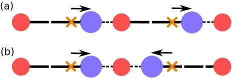
Figure 16: (Color online) In a one-dimensional chain of O-Ti-O-Ti-O, (a) head-to-tail, (b) head-to-head, movement of dipole formed due to the displacement of Ti from the center of O as marked by yellow cross. Red and blue circles corresponding to O and Ti, respectively. Each arrow indicate the movement of the dipole.

Next, we considered the CPB perovskite, which due to its soft bonds and large distortions at even relatively low temperature poses a challenge for atomistic polarizability modeling. Fig. 15 (a) compares the BPM-calculated polarizability with the DFT-calculated polarizability of CPB at 300 K. It can be seen that a high scatter that is much stronger than that for BTO is observed even for the BPM-2^nd data. Similarly, the polarizability trajectories show stronger deviations of the BPM-2^nd results from the DFT results compared to BTO. Comparison of the DFT and BPM-2^nd Raman spectra shows that even in this case, BPM-2^nd results match the peak position of the DFT data. However, the agreement between the relative intensities is quite poor.

Consideration of the perovskite structures and the possible distortions shows that there are several sources of error in the BPM for the modeling of BTO, CPB and other perovskites. The most basic shortcoming is that the strong distortions in these systems may require higher-order terms in the Taylor expansion of bond polarizability to reproduce the DFT results. However, results obtained 3rd- and 4th-order BP models for BTO show only a slight improvement in agreement with DFT results (see SM). Second, similar to the molecular systems, the independent bond approximation of the BPM ignores the effect of Ti-O-Ti and O-Ti-O (Pb-Br-Pb and Br-Pb-Br) angle changes in BTO (CPB). Third, due to its dependence on the bond lengths only, the BPM cannot distinguish between the head-to-head and head-to-tail dipole structures created by the displacements of the B-cations from the centers of their octahedra, as illustrated in Fig. 16. The second and third effects cannot be addressed in the BPM framework due to its fundamental assumption of non-interacting independent contributions of each bond to the total polarizability. In fact, these effects are the primary origin of the disagreement between the DFT and BPM polarizability results for BTO and CBP as demonstrated by the weak improvement provided by the BPM-3^rd and BPM-4^th models for BTO (see SM). Thus, the BPM must be fundamentally modified to include the interactions between bonds to achieve accurate prediction of polarizability for solid-state perovskite systems.

IV CONCLUSIONS

We have investigated the applicability of the bond polarizability model to the modeling of polarizability and Raman spectra using trajectories obtained from MD simulations. We find that BPM including second-order terms generally gives qualitative agreement with the DFT results such that the positions of the Raman peaks are reproduced accurately but their intensities can differ from those obtained by quantum-mechanical calculations. Structures with higher symmetry and with angular vibrations for which the polarizability changes are second-order in the angle change (e.g. CH₄) show much higher accuracy than highly asymmetric molecules (most importantly water) for which the effect of angle changes on the polarizability is linear in the angle change. Similarly, BPM accuracy is much higher for molecules with stiff angular potential energy surface due to $sp^{2}$ bonding (e.g. CH₂O and thiophene). For solid-state BTO perovskite, qualitative accuracy is obtained for the BPM-2^nd model while for the much softer and distorted CPB, BPM shows poor agreement. Due to its simplicity, BPM provides a good starting point for simulations of Raman spectra and can be relied upon to reproduce and interpret strong changes in the experimental Raman spectra. However, the shortcomings of the BPM due to the assumption of non-interacting bonds make it incapable of obtaining quantitative accuracy except for highly symmetric systems and lead to complete failure in case of systems where large deviations from the ground state structure are present. Thus, to enable reliable interpretation of fine features of Raman spectra, it is necessary to develop atomistic models for polarizability that can include the effects of interactions between bonds and angles.

Data Availability

The data used in this work are available from the corresponding author upon reasonable request.

References

- Orlando et al. (2021) A. Orlando, F. Franceschini, C. Muscas, S. Pidkova, M. Bartoli, M. Rovere, and A. Tagliaferro, Chemosensors 9, 262 (2021).
- Long (2002) D. A. Long, The Raman Effect (John Wiley & Sons, Ltd, 2002).
- Gastegger et al. (2017) M. Gastegger, J. Behler, and P. Marquetand, Chem. Sci. 8, 6924 (2017).
- Gaigeot and Sprik (2003) M.-P. Gaigeot and M. Sprik, The Journal of Physical Chemistry B 107, 10344 (2003).
- Thomas et al. (2013) M. Thomas, M. Brehm, R. Fligg, P. Vöhringer, and B. Kirchner, Phys. Chem. Chem. Phys. 15, 6608 (2013).
- Putrino and Parrinello (2002) A. Putrino and M. Parrinello, Phys. Rev. Lett. 88, 176401 (2002).
- Luber et al. (2014) S. Luber, M. Iannuzzi, and J. Hutter, The Journal of Chemical Physics 141, 094503 (2014).
- Mattiat and Luber (2021) J. Mattiat and S. Luber, Journal of Chemical Theory and Computation 17, 344 (2021).
- Lazzeri and Mauri (2003) M. Lazzeri and F. Mauri, Phys. Rev. Lett. 90, 036401 (2003).
- Lussier et al. (2020) F. Lussier, V. Thibault, B. Charron, G. Q. Wallace, and J.-F. Masson, TrAC Trends in Analytical Chemistry 124, 115796 (2020).
- Sommers et al. (2020) G. M. Sommers, M. F. Calegari Andrade, L. Zhang, H. Wang, and R. Car, Phys. Chem. Chem. Phys. 22, 10592 (2020).
- Berger et al. (2024) E. Berger, J. Niemelä, O. Lampela, A. H. Juffer, and H.-P. Komsa, “Raman spectra of amino acids and peptides from machine learning polarizabilities,” (2024), arXiv:2401.14808 [physics.comp-ph] .
- Raimbault et al. (2019) N. Raimbault, A. Grisafi, M. Ceriotti, and M. Rossi, New Journal of Physics 21, 105001 (2019).
- Montero and del Rio (1976) S. Montero and G. del Rio, Molecular Physics 31, 357 (1976).
- (15) M. Cardona, R. Chang, G. Güntherodt, M. Long, and H. Vogt, Light Scattering in Solids II: Basic Concepts and Instrumentation, Topics in Applied Physics (Springer-Verlag Berlin Heidelbergi 1982).
- 199 (1996) in Vibrational Intensities, Vibrational Spectra and Structure, Vol. 22, edited by B. S. Galabov and T. Dudev (Elsevier, 1996) pp. 215–271.
- Liang et al. (2017) L. Liang, A. A. Puretzky, B. G. Sumpter, and V. Meunier, Nanoscale 9, 15340 (2017).
- Wirtz et al. (2005) L. Wirtz, M. Lazzeri, F. Mauri, and A. Rubio, Phys. Rev. B 71, 241402 (2005).
- Luo et al. (2015) X. Luo, X. Lu, C. Cong, T. Yu, Q. Xiong, and S. Ying Quek, Scientific Reports 5, 14565 (2015).
- Umari et al. (2001) P. Umari, A. Pasquarello, and A. Dal Corso, Phys. Rev. B 63, 094305 (2001).
- Hermet et al. (2006) P. Hermet, N. Izard, A. Rahmani, and P. Ghosez, The Journal of Physical Chemistry B 110, 24869 (2006).
- Berger and Komsa (2023) E. Berger and H.-P. Komsa, “Polarizability models for simulations of finite temperature raman spectra from machine learning molecular dynamics,” (2023), arXiv:2310.13310 [cond-mat.mes-hall] .
- Baroni et al. (2001) S. Baroni, S. de Gironcoli, A. Dal Corso, and P. Giannozzi, Rev. Mod. Phys. 73, 515 (2001).
- Giannozzi et al. (2009) P. Giannozzi, S. Baroni, N. Bonini, M. Calandra, R. Car, C. Cavazzoni, D. Ceresoli, G. L. Chiarotti, M. Cococcioni, I. Dabo, A. D. Corso, S. de Gironcoli, S. Fabris, G. Fratesi, R. Gebauer, U. Gerstmann, C. Gougoussis, A. Kokalj, M. Lazzeri, L. Martin-Samos, N. Marzari, F. Mauri, R. Mazzarello, S. Paolini, A. Pasquarello, L. Paulatto, C. Sbraccia, S. Scandolo, G. Sclauzero, A. P. Seitsonen, A. Smogunov, P. Umari, and R. M. Wentzcovitch, Journal of Physics: Condensed Matter 21, 395502 (2009).
- Perdew et al. (2008) J. P. Perdew, A. Ruzsinszky, G. I. Csonka, O. A. Vydrov, G. E. Scuseria, L. A. Constantin, X. Zhou, and K. Burke, Phys. Rev. Lett. 100, 136406 (2008).
- Thompson et al. (2022) A. P. Thompson, H. M. Aktulga, R. Berger, D. S. Bolintineanu, W. M. Brown, P. S. Crozier, P. J. in ’t Veld, A. Kohlmeyer, S. G. Moore, T. D. Nguyen, R. Shan, M. J. Stevens, J. Tranchida, C. Trott, and S. J. Plimpton, Comp. Phys. Comm. 271, 108171 (2022).
- Qi et al. (2016) Y. Qi, S. Liu, I. Grinberg, and A. M. Rappe, Phys. Rev. B 94, 134308 (2016).
- Deluca et al. (2018) M. Deluca, Z. G. Al-Jlaihawi, K. Reichmann, A. M. T. Bell, and A. Feteira, J. Mater. Chem. A 6, 5443 (2018).
- Yuzyuk (2012) Y. I. Yuzyuk, Physics of the Solid State 54, 1026 (2012).