Holistic Memory Diversification for Incremental Learning in Growing Graphs

Abstract

This paper addresses the challenge of incremental learning in growing graphs with increasingly complex tasks. The goal is to continually train a graph model to handle new tasks while retaining its inference ability on previous tasks. Existing methods usually neglect the importance of memory diversity, limiting in effectively selecting high-quality memory from previous tasks and remembering broad previous knowledge within the scarce memory on graphs. To address that, we introduce a novel holistic Diversified Memory Selection and Generation (DMSG) framework for incremental learning in graphs, which first introduces a buffer selection strategy that considers both intra-class and inter-class diversities, employing an efficient greedy algorithm for sampling representative training nodes from graphs into memory buffers after learning each new task. Then, to adequately rememorize the knowledge preserved in the memory buffer when learning new tasks, we propose a diversified memory generation replay method. This method first utilizes a variational layer to generate the distribution of buffer node embeddings and sample synthesized ones for replaying. Furthermore, an adversarial variational embedding learning method and a reconstruction-based decoder are proposed to maintain the integrity and consolidate the generalization of the synthesized node embeddings, respectively. Finally, we evaluate our model on node classification tasks involving increasing class numbers. Extensive experimental results on publicly accessible datasets demonstrate the superiority of DMSG over state-of-the-art methods.

1 Introduction

Graphs, owing to their flexible relational data structures, are widely employed for many applications in various domains, including social networks [1, 2], recommendation systems [3, 4], and bioinformatics [5]. With the increasing prevalence of graph data, graph-based models like Graph Neural Networks (GNNs) have gained significant attention due to their ability to capture complex structural relationships and those dynamic variants also demonstrate remarkable inductive capabilities on growing graph data [6, 7, 8]. However, as the growing graph in Figure 1 shows, when new nodes are added, the associated learning tasks can become increasingly complex. For example, the graph models on academic networks might need to predict the topics of papers in highly dynamic research areas where the topic rapidly emerges, and those on recommendation networks might need to continually adapt to new user preferences. Recent research on the inductive capability and adaptability of GNNs often remains limited to a specific task [9, 10, 11] and cannot be readily applied to incremental tasks. Moreover, it is often inefficient to train an entirely new model from scratch every time a new learning task is introduced. In recent years, model reuse via incremental learning [12, 13], also known as continual learning or lifelong learning, has led to exploring more economically viable pipelines, enabling the model to adaptively learn new tasks while maintaining the knowledge from old tasks.

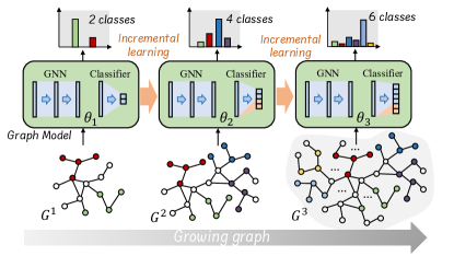
Figure 1: An example of incremental learning in growing graphs, where nodes with distinct labels are shaded in various colors. The number of classes expands as the graph grows, causing increasingly complex classification tasks.

The main challenge of incremental learning on graphs lies in mitigating catastrophic forgetting. As the graph model learns from a sequence of tasks on evolving graphs, it tends to forget the information learned from previous tasks when acquiring knowledge from new tasks. One prevalent approach to address this issue is the memory replay method, a human-like method that typically maintains a memory buffer to store the knowledge gained from previous tasks. When learning a new task, the model not only focuses on the current information but also retrieves and re-learns from memory, preventing the model from forgetting what was learned previously as it takes on new tasks. This method has two major focuses to address on graphs: (1) How to select knowledge from old graphs to form more high-quality memory buffers? Existing methods usually select representative training samples as knowledge. However, determining which nodes in the graph are more representative is difficult and usually a time-consuming process. Furthermore, most methods [14, 15] select samples all into one same buffer without considering the inter-class differences between various previous tasks, which may degrade the quality of preserved knowledge. (2) How to effectively replay the limited buffer knowledge to enhance the model’s memorization of previous tasks? Due to constraints related to memory and training expenses, the samples chosen for the buffer are often limited. Many methods [16, 17] concentrate on memory selection, neglecting to broaden the boundaries of memory within the buffer, resulting in a discount in replay. Finding an effective way to replay knowledge from these limited nodes is critical to incremental learning in graphs.

In this paper, we propose a novel Diversified Memory Selection and Generation (DMSG) method on incremental learning in growing graphs, devised to tackle the above challenges. we consider that selecting diversified memory helps in Comprehensive Knowledge Retention: we apply a heuristic diversified memory selection strategy that takes into account both intra-class and inter-class diversities between nodes. By employing an efficient greedy algorithm, we selectively sample representative training nodes from the growing graph, placing them into memory buffers after completing each new learning task. Furthermore, we explore the memory diversification in memory reply for Enhanced Knowledge Memorization: we introduce a generative memory replay method, which first leverages a variational layer to produce the distribution of buffer node embeddings, from which synthesized samples are drawn for replaying. We incorporate an adversarial variational embedding learning technique and a reconstruction-based decoder. These are designed to preserve the integrity of the information and strengthen the generalization of the synthesized node embeddings on the label space, ensuring the essential knowledge is carried over accurately and effectively.

The main contributions can be summarized as follows: (1) We propose a novel and effective memory buffer selection strategy that considers both the intra-class and inter-class diversities to select representative nodes into buffers. (2) We propose a novel memory replay generation method on graphs to generate diversified and high-quality nodes from the limited real nodes in buffers, exploring the essential knowledge and enhancing the effectiveness of replaying. (3) Extensive experiments on various incremental learning benchmark graphs demonstrate the superiority of the proposed DMSG over state-of-the-art methods.

2 Problem Formulation

In this section, we present the formulation for the incremental learning problem in growing graphs. Generally, a growing graph is represented by a sequential of $m$ snapshots: $G=\{G^{1},G^{2},...,G^{m}\}$, and each snapshot corresponds to the inception of a new task, represented as $\mathcal{T}=\{\mathcal{T}^{1},\mathcal{T}^{2},...,\mathcal{T}^{m}\}$. Each graph $G^{i}$ is evolved from the previous graph $G^{i-1}$, i.e., $G^{i-1}\subset G^{i},\forall i\in 2,...,m.$, and each learning task $\mathcal{T}^{i}$ is more complex than the previous task $\mathcal{T}_{i-1}$. This paper specifies the learning tasks to classification tasks, i.e., the number of classes increases alongside graph growth, increasing the task complexity. In this scenario, we aim to continually learn a model $f(\theta)$ on $\mathcal{T}$. For the $t$-th step, the task $\mathcal{T}^{t}$ incorporates a training node set $\mathcal{V}^{t}$ with previously unseen labels (i.e., novel classes), where each vertex $v_{i}\in\mathcal{V}^{t}$ has the label $y_{i}\in\mathcal{Y}^{t}$, and $\mathcal{Y}^{t}=\{y^{t}_{1},y^{t}_{2},...,y^{t}_{n}\}$ is the set of $n$ novel classes. The task $\mathcal{T}^{t}$ is to train the $f(\theta):v_{i}\rightarrow\bigcup_{j=1}^{t}\mathcal{Y}^{j}$ to ensure it can infer well on the current novel classes while preventing catastrophic forgetting of the inference ability on previous classes.

Jointly Incremental Learning. This is a straightforward solution for the problem, which collects training nodes of all classes of previous tasks to train $f(\theta)$ in each step. This treats the accumulated tasks $\{\mathcal{T}^{1},\mathcal{T}^{2},...,\mathcal{T}^{t}\}$ as a whole new task and retrains the model from scratch. However, this solution is inefficient because it leads to redundant training of labeled nodes and creates computational challenges due to the growing graph size. Conversely, the buffer memory replay model offers a more practical solution.

Memory Replay for Incremental Learning. This method, instead of gathering all previous training nodes, maintains buffers $\mathcal{B}$ that store a small yet representative subset of training nodes for each class of previous tasks. The objectives can be formulated as follows:

$$\mathcal{L}=\underbrace{\sum_{v_{i}\in\mathcal{V}^{t}}\ell^{t}(f(v_{i};\theta),y_{i})}_{\text{Loss on new tasks}}+\underbrace{\lambda\sum_{j=1}^{K}\sum_{v_{k}\in\mathcal{B}_{j}}\ell^{t}(f(v_{k};\theta),y_{k})}_{\text{Memory replay on previous tasks}},$$ (1)

where $\ell^{t}$ is the loss function on the accumulated all class set, $K=|\bigcup_{i=1}^{t-1}\mathcal{Y}^{i}|$ is the number of previous classes, the $\lambda$ is a balance hyper-parameter, and $\mathcal{B}_{j}$ is the buffer for the $j$-th class. The second term ensures the representative training nodes from previous classes are included in the current training phase, efficiently mitigating the risk of catastrophic forgetting of previous classes. Also, the size of $\mathcal{B}_{j}$ is much smaller than the total node number of class $j$. Thus, the number of training nodes required is significantly lower than joint training, leading to a substantial increase in efficiency.

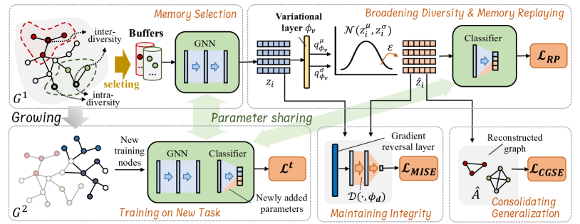
Figure 2: The framework of DMSG. In this instance, the graph model underwent training on a 2-class node classification task on $G^{1}$. Two new classes of nodes are added to form $G^{2}$. Certain nodes of the previous two classes are first selected into buffers. Then, the model is further trained on the two new classes of nodes and buffers to perform incremental learning.

3 Methodology

Without loss of generality, we choose the plain GCN model followed by a classifier head as the backbone of $f(\theta)$, which can encode each node $v_{i}$ into an embedding $z_{i}$ and a probability $p_{i}$. As shown in Figure 2, initially, this model is trained on the graph $G_{1}$. When the $t$-th task introducing new classes arrives, we first extend new parameters (highlighted as the yellow segment) into the last layer of the classifier, ensuring the output probabilities encompass the previous and newly introduced classes. To facilitate continual training of $f(\theta)$, we leverage the memory replay framework, which incorporates both the Heuristic Diversified Memory Selection (Section 3.1) and the Diversified Memory Generation Replay (Section 3.2).

Motivation. Consider $p(G_{<t})$ as the true data distribution of graphs from prior $t-1$ tasks, and $q(\mathcal{B}_{<t})$ as the data distribution encapsulated within the memory replay buffers $\mathcal{B}$ sampled from $G_{<t}$. To understand the efficacy of the buffer diversity in incremental learning scenarios, we engage in a theoretical examination to indicate that a high diversity within $\mathcal{B}$ ensures that the empirical loss $\mathcal{L}(\theta)$ over $\mathcal{B}$ closely mirrors the total expected loss $\mathcal{L}(\theta)$ over $p(G_{<t})$.

Theorem 1.

Let the loss function $\mathcal{L}(\theta,x)$ be $\beta$-Lipschitz continuous in respect to the input $x$. Under this condition, the discrepancy between the expected loss under the true data distribution $p(G_{<t})$ and that under the replay buffer distribution $q(\mathcal{B}_{<t})$ is bounded as follows:

$$\left|\mathbb{E}_{v\sim p(G_{<t})}[\mathcal{L}(\theta,v)]-\mathbb{E}_{v\sim q(\mathcal{B}_{<t})}[\mathcal{L}(\theta,v)]\right|\leq\beta\cdot W(p(G_{<t}),q(\mathcal{B}_{<t})),$$ (2)

where $W(p,q)$ denotes the Wasserstein distance between distributions $p$ and $q$, defined by: $W(p,q)=\inf_{\gamma\in\Gamma(p,q)}\mathbb{E}_{(v,v^{\prime})\sim\gamma}[d(v,v^{\prime})],$ and $\Gamma(p,q)$ represents the set of all possible joint distributions (couplings) that can be formed between $p$ and $q$.

Assume that both $p(G_{<t})$ and $q(\mathcal{B}_{<t})$ follow Gaussian distributions with means $\mu_{p},\mu_{q}$ and covariance matrices $\Sigma_{p},\Sigma_{q}$ respectively. Thus, the squared 2-Wasserstein distance between two Gaussian distributions is given by:

$$W_{2}^{2}(\mathcal{N}(\mu_{p},\Sigma_{p}),\mathcal{N}(\mu_{q},\Sigma_{q}))=\|\mu_{p}-\mu_{q}\|^{2}+\operatorname{Tr}(\Sigma_{p}+\Sigma_{q}-2(\Sigma_{p}^{1/2}\Sigma_{q}\Sigma_{p}^{1/2})^{1/2}).$$ (3)

Since the $\Sigma$ measure the distribution diversity and $\mathcal{B}_{<t}$ is the subset of $\mathcal{G}_{<t}$ and is typically less diverse. Assuming the sampling strategy is unbiased upon means. As the $\mathcal{B}_{<t}$ more diversified, $\Sigma_{q}\rightarrow\Sigma_{p}$, leading to the Wasserstein distance decreases. Based on Theorem 1, the discrepancy between the expected loss under true distribution and the buffer distribution becomes less, making the optimization on the buffer more closely approximate the optimization on all previous graph data.

3.1 Heuristic Diversified Memory Selection

Based on the above motivations. For memory selection, to ensure that the selected nodes are adequately diverse with respect to the classification task, we consider the two perspectives: P1: the nodes within the same buffer should exhibit sufficient diversity to faithfully represent disparate regions of their corresponding areas. Also, P2: the inter-class distance between nodes residing in distinct buffers should be maximized to facilitate the model to delineate clear classification boundaries. Thus, we introduce the concepts of intra-diversity and inter-diversity for the buffers. Our goal is to select the buffer $\mathcal{B}_{i}$ corresponding to the $i$-th class of training nodes based on the following criteria:

$$\mathcal{B}_{i}=\arg\max\limits_{\mathcal{B}_{i}\subset\mathcal{C}_{i}}\sum\limits_{v\in\mathcal{B}_{i}}[\underbrace{\mathcal{A}(v,\mathcal{B}_{i})}_{\text{intra-diversity}}+\underbrace{\frac{1}{K-1}\sum_{\begin{subarray}{c}j=1,j\neq i,\mathcal{B}_{j}\subset\mathcal{C}_{j}\end{subarray}}^{K}\mathcal{A}(v,\mathcal{B}_{j})}_{\text{inter-diversity}}],$$ (4)

where $\mathcal{C}_{i}$ is set of $i$-th class of training nodes, $\mathcal{A}(v,\mathcal{B}_{i},G^{t})$ denotes the distance measure between node $v$ and $\mathcal{B}_{i}$ in the current graph $G^{t}$, which we define as the L2-norm distance on probabilities between node $v$ and its closest node in $\mathcal{B}_{i}$. While the measure can be defined as any topological distance, such as the shortest path, we use probability distance because it offers finer resolution, reduced noise towards tasks, and computational efficiency. The first term quantifies the intra-diversity within the buffer $\mathcal{B}_{i}$, reflecting the variations among its own nodes, while the second term quantifies the inter-diversity between $\mathcal{B}_{i}$ and other buffers, illustrating the differences between the nodes of $\mathcal{B}_{i}$ and those belonging to other buffers.

Heuristic Greedy Solution. However, achieving this objective for selecting different classes of buffers is an NP-hard problem. This kind of problem is usually addressed using heuristic methods [18]. Thus, we introduce a greedy algorithm to sample representative training nodes when new tasks are introduced. Specifically, suppose $\mathcal{V}^{t}=\bigcup_{i=K+1}^{K+n}\mathcal{C}^{t}_{i}$ is the training nodes of $t$-th task and $\mathcal{C}^{t}_{i}$ is the training set corresponding to the $i$-th novel class. We have previously selected buffers $\{\mathcal{B}_{i}\}_{i=1}^{K}$ in previous $t-1$ tasks, where $K$ and $n$ are the numbers of previous classes and novel classes, respectively. Then, the greedy selection strategy is defined in the Algorithm 1, where $\mathbb{D}(\mathcal{B}_{i})=\sum_{v\in\mathcal{B}_{i}}(\mathcal{A}(v,\mathcal{B}_{i})+\frac{1}{K-1}\sum_{j=1,j\neq i,\mathcal{B}_{j}\subset\mathcal{C}_{j}}^{K}\mathcal{A}(v,\mathcal{B}_{j}))$ is the set score function defined on the buffer set $\mathcal{B}_{i}$ of the $i$-th class, $\triangle_{\mathbb{D}}(v|\mathcal{B}_{i})$ is the gain of $f$ choosing $v$ into $\mathcal{B}_{i}$, and $v*$ is the chosen node using the greedy strategy. In greedy Algorithm 1, the core idea is to make the currently best choice of buffer nodes at every step, hoping to obtain the global optimal solution for the objective Eq.4 through this local optimal choice.

Input: $\{\mathcal{B}_{i}\}_{i=1}^{K}$. // buffers of previous tasks.

$\{\mathcal{C}^{t}_{i}\}_{i=K+1}^{K+n}$. // training node sets of novel classes of current tasks.

$f(\theta)$. // Model after trained on the $(t-1)$-th task.

Output: $\{\mathcal{B}_{i}\}_{i=1}^{K+n}$ // updated buffers.

/* Initializing. */

1 Create empty buffer $\{\mathcal{B}_{i}\}_{i=K+1}^{K+n}$.

2 for $i$ from $K+1$ to $K+n$ do

3      Select one node with highest output probability on the $i$-th label from $\mathcal{C}^{t}_{i}$ into $\mathcal{B}_{i}$ via $f(\theta)$.

4 end for

/* Greedy Selecting. */

5 repeat

6       for $i$ from $K+1$ to $K+n$ do

7            $\triangle_{\mathbb{D}}(v|\mathcal{B}_{i})=\mathbb{D}(\mathcal{B}_{i}\cup v)-\mathbb{D}(\mathcal{B}_{i}),$

8             $v^{*}=\arg\max_{\mathcal{C}_{i}\textbackslash\mathcal{B}_{i}}\triangle_{\mathbb{D}}(v|\mathcal{B}_{i})$.

9             Add $v^{*}$ into $\mathcal{B}_{i}$.

10       end for

11      

12until $b$ nodes are sampled in each buffer;

Algorithm 1 Heuristic Buffer Selection

Below, we give a Proposition of approximation guarantee of our greedy algorithm.

Proposition 1.

(Greedy Approximation Guarantee of Algorithm 1). The greedy Algorithm 1 that sequentially adds elements to an initially empty set based on the largest marginal gain $\triangle_{\mathbb{D}}$ under a cardinality constraint provides a solution $\mathcal{B}^{*}_{i}$ that is at least $(1-\frac{1}{e})$ times the optimal solution, i.e.,

$$f(\mathcal{B}^{*}_{i})\geq\left(1-\frac{1}{e}\right)\cdot f(OPT),$$ (5)

where $OPT$ represents the optimal solution of the buffer set $\mathcal{B}_{i}$.

Proof.

The above Proposition can be derived from the Greedy Approximation Guarantee for Monotonic and Submodular Functions [19] (proof can be found in Theorem 1 in the Appendix), given that our function $f$ is both monotonic (from Lemma 1) and submodular (from Lemma 2). The greedy algorithm is guaranteed to produce a solution that is at least $(1-\frac{1}{e})$ times the optimal solution. ∎

Time Complexity Analysis. For each buffer of the $t$-th task, there are $b$ sampling steps where $b$ is the size of the buffers. Each sampling can be done in $O((K+n)*|\mathcal{C}^{t}_{i}|)$, by determining distances and making comparisons. Thus, the overall complexity of selecting each buffer is $O(b(K+n)*|\mathcal{C}^{t}_{i}|)$. Note that $b$ (the buffer size) and $K+n$ (the total number of classes up to $t$-th task) are typically much smaller than $|\mathcal{C}^{t}_{i}|$, ensuring the efficiency of the algorithm.

3.2 Diversified Memory Generative Replay

During training for the $t$-th task $\mathcal{T}^{t}$, the stored representative nodes in the buffers $\{\mathcal{B}_{i}\}_{i=1}^{K}$ from previous $t-1$ tasks are also recalled to reinforce what the model has previously learned, known as memory replay. However, the limited buffer size still presents challenges: C1: the stored knowledge may be constrained and might not encompass the full complexity of previous tasks, leading to a potential bias in replaying, and C2: the training process can become difficult as the model may easily overfit to the limited nodes in the buffers, undermining its ability to generalize across different tasks. Thus, we proposed the Diversified Memory Generation Replay to address the above problems.

Broadening Diversity of Buffer Node Embeddings. Specifically, the embeddings of the buffer nodes are first subjected to a variational layer, which aims to create more nuanced representations that encapsulate the inherent probabilistic characteristics of nodes. Let $z_{i}\in\mathbb{R}^{h}$ denote the embedding of node $v_{i}\in\mathcal{B}_{j},1\leq j\leq K$, where $h$ is the hidden dimension. Specifically, we treat the nodes in the buffers as the observed samples $\mathcal{V}_{ob}$ drawn from the ground-truth distribution of the previous nodes:

$$Z=\bigcup_{j=1}^{K}\bigcup_{v_{i}\in\mathcal{B}_{j}}\{z_{i}\}\in\mathbb{R}^{(K\times b)\times h}\xlongequal{\text{def}}\mathcal{V}_{ob}.$$ (6)

The node variable $\widehat{Z}$ is drawn from the variational network layer $q_{\phi_{v}}(\widehat{Z}|Z)$ with parameters $\phi_{v}$. Specifically, $q_{\phi_{v}}$ outputs the mean and variance of the node embeddings distributions respectively, expressed as $Z^{\mu}=q_{\phi_{v}}^{\mu}(Z)$ and $Z^{\sigma}=q_{\phi_{v}}^{\sigma}(Z)$, where $q_{\phi_{v}}^{\mu}(\cdot)$ is the identity function and $q_{\phi_{v}}^{\sigma}(\cdot)$ is a Liner layer followed with a Relu activation layer. Then we use the reparameterization technique to sample from $\mathcal{N}(Z^{\mu},Z^{\sigma})$, expressed as $\widehat{Z}=Z^{\mu}+Z^{\sigma}\odot\epsilon$, where $\widehat{Z}\in\mathbb{R}^{h}$ and $\epsilon$ is drawn from standard normal distributions. Thus, we define the generated samples as $\mathcal{V}_{ge}$. The variational operation augments the diversity of observed buffer nodes $\mathcal{V}_{ob}$, empowering the model to explore more expansive distribution spaces.

Maintaining Integrity of Synthesized Embeddings. Then, we further propose to maintain the integrity of these variational node embeddings to prevent them from deviating too far, which implies that while the generated embeddings should exhibit diversity, they must remain similar to the ground-truth ones. Specifically, we adopt an adversarial learning strategy [20]. We introduce an auxiliary discriminator, $\mathcal{D}:\mathbb{R}^{h}\rightarrow\mathbb{R}^{1}$ with parameters $\phi_{d}$, tasked with distinguishing the original embeddings and the variational embeddings of nodes. In contrast, the model is learned to generate diversified variational node embeddings from the original ones, meanwhile ensuring the authenticity of synthesized variational node embeddings. Thus, the learning objective is defined as follows:

$$\mathcal{L}_{MISE}=\min_{\theta,\phi_{v}}\mathbb{E}_{z_{i}\sim Z}\mathbb{E}_{q_{\phi_{v}}(\hat{z}_{i}|z)} \left[\max_{\phi_{d}}\text{ }\ell_{\mathcal{D}}(z_{i},\hat{z}_{i})\vphantom{\max_{\phi_{d}}}\right],$$ (7)

where $\ell_{\mathcal{D}}$ is a negative binary cross-entropy loss function on the variational and original node embeddings, defined as:

$$\ell_{\mathcal{D}}(z_{i},\hat{z}_{i})=\log\mathcal{D}(z_{i},\phi_{d})+\log\left(1-\mathcal{D}(\hat{z}_{i},\phi_{d})\right).$$ (8)

The min-max adversarial learning strategy involves training the domain discriminator to distinguish whether the node embeddings are synthesized or original while simultaneously enforcing a constraint on the model to generate indistinguishable node embeddings from the domain discriminator. This interplay aims to yield synthesized node embeddings that are more comprehensive and maintain integrity. It leverages the strengths of generative methods for increased representational complexity of buffer nodes to address C1. Simultaneously, it employs adversarial learning and regularization to ensure this expansion does not lead to distortions.

Consolidating Generalization of Synthesized Embeddings. Furthermore, to adequately capture the node relationships within the variational node embeddings, we use the variational node embeddings to generate a reconstructed graph on the buffer nodes. As the buffer nodes are sampled from disparate regions, and the initial connections between them are sparse, we instead employ the ground-truth label to build the reconstructed graph. Specifically, nodes sharing the same labels are linked, while those with different labels are not connected. The reconstructed graph is denoted as $\widehat{A}\in\mathbb{R}^{Kb\times Kb}$ and the decoder loss is defined as:

$$\mathcal{L}_{CGSE} =-\mathbb{E}_{q_{\phi_{v}}(\widehat{Z}|Z)}[\log p(\widehat{A}|\widehat{Z})]+\text{KL}(q_{\phi_{v}}(\hat{z}_{i}|z)||p(\hat{z}_{i}))$$ (9)

$$=-\mathbb{E}_{\hat{z}_{i},\hat{z}_{j}\sim\widehat{Z}}\left[\widehat{A}_{ij}\log\widehat{p}_{ij}+\widehat{A}_{ij}\log(1-\widehat{p}_{ij})\right]+\text{KL}(q_{\phi_{v}}(\hat{z}_{i}|z)||p(\hat{z}_{i})),$$

where $p(\widehat{A}|\widehat{Z})$ is the probability of reconstructing $\widehat{A}$ given the latent variational node embedding matrix $\widehat{Z}$, following a Bernoulli distribution. $\widehat{p}_{ij}$ is the probability of an edge between nodes $i$ and $j$, defined as: $\widehat{p}_{ij}=\text{sigmoid}(\widehat{z}_{i}^{T}\cdot\widehat{z}_{j})$. The second term in Eq. 7 is a distribution regularization term, which enforces the variational distribution $q_{\phi_{v}}(\hat{z}_{i}|z)$ of each node to be close to a prior distribution $p(\hat{z}_{i})$, which we assume is a standard Gaussian distribution. $\text{KL}(\cdot)$ represents the Kullback-Leibler (KL) divergence. The detailed derivation of $\mathcal{L}_{CGSE}$ is in the Appendix.

The reconstruction objective incorporates both the inter-class and intra-class relationships between nodes in buffers. This loss facilitates the learning of variational node embeddings with well-defined classification boundaries, further bolstering the model’s generalization on the label space. As such, the method can effectively address C2.

Replaying on Generated Diversified Memory. Finally, we define the reply objective on the variational embeddings of buffer nodes, rather than the original embeddings, expressed as:

$$\mathcal{L}_{RP}=\sum_{j=1}^{K}\sum_{v_{i}\in\mathcal{B}_{j}}\ell^{t}(\hat{z_{i}},y_{i}).$$ (10)

Note that the variational operation regenerates synthetic buffer node embeddings with the same size as original embeddings in each training step, i.e., $|\mathcal{V}_{ge}|\equiv|\mathcal{V}_{ob}|$, broadening the diversity of memory while guaranteeing the efficiency of the buffer replay.

3.3 Overall Optimization

Combining the new task loss $\mathcal{L}^{t}=\sum_{v_{i}\in\mathcal{V}^{t}}\ell^{t}(f(v_{i};\theta),y_{i})$ and the above memory replay losses, the overall optimization objective can be written as follows:

$$\min_{\theta}\mathcal{L}^{t}+\min_{\theta,\phi_{v}}\left\{\lambda_{1}\mathcal{L}_{RP}+\lambda_{2}\max_{\phi_{d}}\{\mathcal{L}_{MISE}\}+\lambda_{3}\mathcal{L}_{CGSE}\right\},$$ (11)

where $\lambda_{1}$, $\lambda_{2}$ and $\lambda_{3}$ is the loss weights.

Synchronized Min-Max Optimizating. A gradient reversal layer (GRL) [21] is introduced between the variational embedding and the auxiliary discriminator so as to conveniently perform min-max optimization on $\theta,\phi_{v}$ and $\phi_{d}$ under $\mathcal{L}_{adv}$ in the same training step. GRL acts as an identity transformation during the forward propagation and changes the signs of the gradient from the subsequent networks during the backpropagation.

Scaliability on Large-Scale graphs. In practice, in each training step, training the proposed method on the entire graph and buffer at once may not be practical, especially for large-scale graphs. Following methods like GraphSAGE [9] and GraphSAINT [22], we adopt a mini-batch optimization strategy. We sample a multi-hop neighborhood for each node and set two kinds of batch sizes, $B^{\text{new}}$ and $B^{\text{buffer}}$, for the new task and replay losses in Eq. 11, respectively. The ratio of these batch sizes corresponds to the ratio between the total training nodes in the new task and the buffer.

4 Experiments

Experiment Setup. In this section, we describe the experiments we perform to validate our proposed method. We use the four growing graph datasets, CoraFull, OGB-Arxiv, Reddit, and OGB-Products, introduced in Continual Graph Learning Benchmark (CGLB) [23]. These graphs contain 35, 20, 20, and 23 sub-graphs, respectively, where each sub-graph corresponds to new tasks with novel classes. For baselines, we establish the upper bound baseline Joint defined in Section 2. The lower bound baseline Fine-tune employs only the newly arrived training nodes for model adaptation withour memory replay. Then, we set multiple continual learning models for graph as baselines, including EWC [24], MAS [25], GEM [26], LwF [27], TWP [28], ER-GNN [16], and SEM [14]. For a fair comparison, the backbone is set as two layers and the hidden dimension as 256 for all baselines. For evaluation metric, we first report the accuracy matrix $M^{acc}\in\mathbb{R}^{T\times T}$, which is lower triangular where $M^{acc}_{i,j}(i\geq j)$ represents the accuracy on the $j$-th tasks after learning the task $i$. To derive a single numeric value after learning all tasks, we report the Average Accuracy (AA) $\frac{1}{T}\sum_{i=1}^{T}M^{acc}_{T,i}$ and the Average Forgetting (AF) $\frac{1}{T-1}\sum_{i=1}^{T-1}M^{acc}_{T,i}-M^{acc}_{i,i}$ for each task after learning the last task. For detailed introduction to dataset description, compared methods, evaluation metrics, and hyperparameter setting, please refer to Appendix.

Overall Comparison. This experiment aims to answer: How is DMSG’s performance on the continual learning on graphs? We compare DMSG with various baselines in the class-incremental continual learning task and report the experimental results in Table 1. Initially, we observe that DMSG attains a significant margin over other baseline methods across all datasets. Certain baseline methods demonstrate exceedingly poor results. This can be attributed to the difficulty of the problem, which involves more than 20 timesteps’ continual learning. When the model forgets intermediate tasks, errors are cumulatively compounded for subsequent tasks, potentially leading to the model easily collapsing. However, our model addresses this challenge through superior buffer selection and replay training strategies, effectively avoiding catastrophic problems. Among the various baselines, the most comparable method to DMSG is SEM. Our method outperforms SEM mainly because we improve the buffer selection strategy, i.e., instead of random selection, we employ distance measures to choose more representative nodes for each class. Additionally, the variational replay method enables our model to effectively learn the data distribution from previous tasks. When compared to Joint, DMSG achieves comparable results, demonstrating its effectiveness in preserving knowledge from previous tasks, even with limited training samples. Notably, our method outperforms Joint on the Reddit dataset, and also exhibits a positive AF. This improvement can be attributed to the proposed buffer selection strategy, which can select representative nodes, in other words, eliminate the noise nodes, and thereby enhancing the results.

Table 1: The model performance comparisons( $\uparrow$: higher is better, Joint is the upper bound).

Methods	CoreFull		OGB-Arxiv		Reddit		OGB-Products
	AA/% $\uparrow$	AF/% $\uparrow$	AA/% $\uparrow$	AF/% $\uparrow$	AA/% $\uparrow$	AF/% $\uparrow$	AA/% $\uparrow$	AF/% $\uparrow$
Fine-tune	3.5$\pm$0.5	-95.2$\pm$0.5	4.9$\pm$0.0	-89.7$\pm$0.4	5.9$\pm$1.2	-97.9$\pm$3.3	3.4$\pm$0.8	-82.5$\pm$0.8
EWC	52.6$\pm$8.2	-38.5$\pm$12.1	8.5$\pm$1.0	-69.5$\pm$8.0	10.3$\pm$11.6	-33.2$\pm$26.1	23.8$\pm$3.8	-21.7$\pm$7.5
MAS	12.3$\pm$3.8	-83.7$\pm$4.1	4.9$\pm$0.0	-86.8$\pm$0.6	13.1$\pm$2.6	-35.2$\pm$3.5	16.7$\pm$4.8	-57.0$\pm$31.9
GEM	8.4$\pm$1.1	-88.4$\pm$1.4	4.9$\pm$0.0	-89.8$\pm$0.3	28.4$\pm$3.5	-71.9$\pm$4.2	5.5$\pm$0.7	-84.3$\pm$0.9
TWP	62.6$\pm$2.2	-30.6$\pm$4.3	6.7$\pm$1.5	-50.6$\pm$13.2	13.5$\pm$2.6	-89.7$\pm$2.7	14.1$\pm$4.0	-11.4$\pm$2.0
LwF	33.4$\pm$1.6	-59.6$\pm$2.2	9.9$\pm$12.1	-43.6$\pm$11.9	86.6$\pm$1.1	-9.2$\pm$1.1	48.2$\pm$1.6	-18.6$\pm$1.6
ER-GNN	34.5$\pm$4.4	-61.6$\pm$4.3	30.3$\pm$1.5	-54.0$\pm$1.3	88.5$\pm$2.3	-10.8$\pm$2.4	56.7$\pm$0.3	-33.3$\pm$0.5
Joint	81.2$\pm$0.4	-3.3$\pm$0.8	51.3$\pm$0.5	-6.7$\pm$0.5	97.1$\pm$0.1	-0.7$\pm$0.1	71.5$\pm$0.1	-5.8$\pm$0.3
DMSG	77.8$\pm$0.3	-0.5$\pm$0.5	50.7$\pm$0.4	-1.9$\pm$1.0	98.1$\pm$0.0	0.9$\pm$0.1	66.0$\pm$0.4	-0.9$\pm$1.6

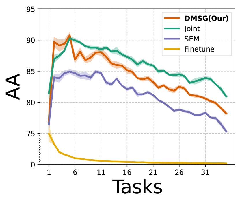
(a) CoraFull

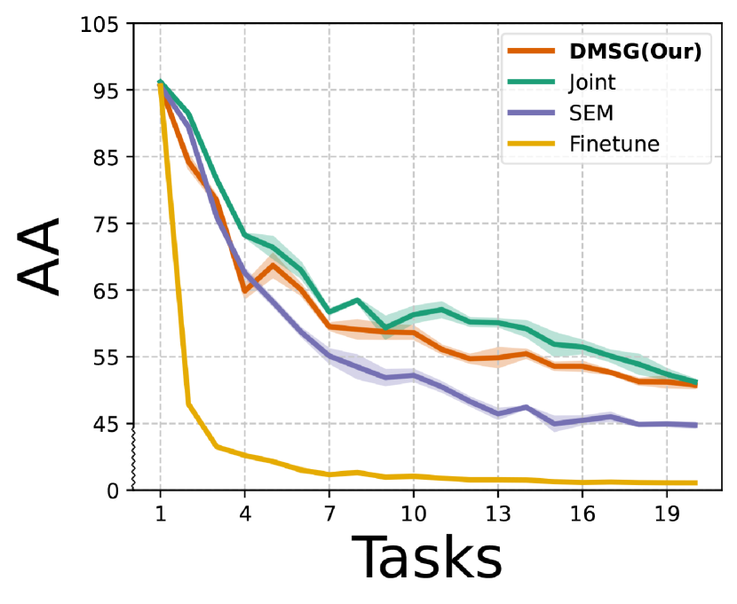
(b) OGB-Arxiv

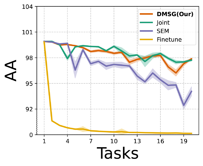
(c) Reddit

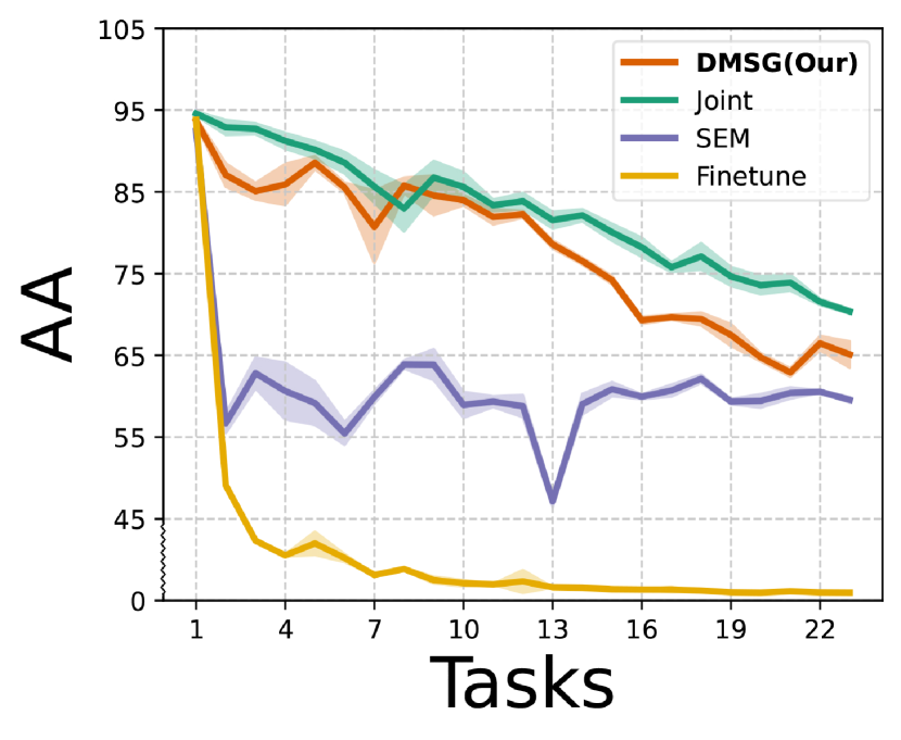
(d) OGB-Product

Figure 3: Dynamics of the average accuracy during incremental learning on different growing graphs.

In-Depth Analysis of Continuous Performance.

This experiment aims to answer: How does DMSG’s fine-grained performance evolve after continuously learning each task? To present a more fine-grained demonstration of the model’s performance in continual learning on graphs, we analyzed the average performance across all previous tasks each time a new task was learned. The comparative results of Fine-tune, Joint, DMSG, and the top-performing baseline, SEM, are depicted in Figure 3. The curve represents the model’s performance after $t$ in terms of AA on all previous $t$ tasks. Also, we visualize the accuracy matrices of DMSG and SEM on the OGB-Arxiv and OGB-Product datasets. The results are presented in Figure 4. In these matrices, each row represents the performance across all tasks upon learning a new one, while each column captures the evolving performance of a specific task as all tasks are learned sequentially. In the visual representation, lighter shades signify better performance, while darker hues indicate inferior outcomes. From the results, we observed that as the number of tasks increases, the learning objectives grow increasingly complex, resulting in a reduction in performance across all examined methods, including Joint. That is because as tasks accumulate and the learning objectives become multifaceted, it becomes challenging for models to maintain optimal performance across all classes. Notably, the Fine-Tuning strategy experienced a substantial decline, with the model collapsing with the arrival of merely two new tasks, demonstrating that catastrophic forgetting occurs almost immediately when the model fails to access previous memories. This reinforces the need for effective continual learning techniques on the growing graphs where new tasks frequently emerge. While the performance drop was observed across all methods, DMSG demonstrated resilience and outperformed the top-performing baseline SEM. Also, DMSG predominantly displays lighter shades across the majority of blocks compared to SEM in Figure 4. Moreover, its competitive performance with Joint in specific datasets signifies its robustness and capability. This could be attributed to diversified memory selection and generation in DMSG that not only help in mitigating forgetting but also in adapting efficiently to new tasks.

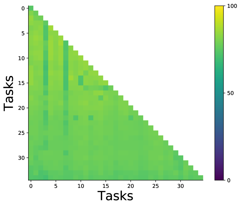
(a) CoraFull (SEM)

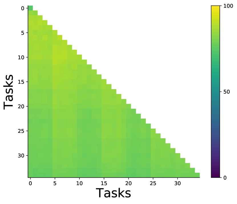
(b) CoraFull (DMSG)

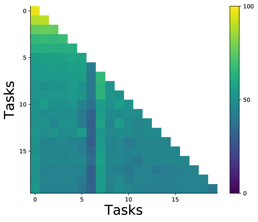
(c) OGB-Arxiv (SEM)

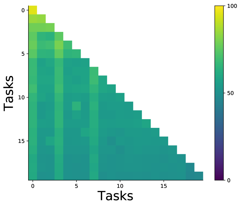
(d) OGB-Arxiv (DMSG)

Figure 4: Accuracy matrices of DMSG and SEM in different datasets.

Component Analysis of Memory Replay. This experiment aims to answer: Are all the proposed memory replay technologies of DMSG have the claimed contribution to continual learning? To investigate the distinct contributions of the diversified memory generation replay method, we conducted an ablation study on it. We design three variant methods for DMSG to verify the effectiveness of adversarial synthesized embedding learning and the graph reconstruction optimization objective. w/o $\mathcal{L}_{MISE}$: This variant excludes the adversarial learning loss for maintaining the integrity of synthesized embeddings. ; w/o $\mathcal{L}_{CGSE}$: This variant excludes the graph reconstruction loss on variational embeddings for consolidating their generalization to label space; w/o all: both losses were removed, and as a result, the model operates without any variational embeddings and just replays the original nodes in the memory buffers. From the results in Table 2, we can observe when both $\mathcal{L}_{MISE}$ and $\mathcal{L}_{CGSE}$ are removed (w/o all), the performance is the lowest across all datasets. Also, a progressive improvement is observed as individual components in the model.

Table 2: The ablation study of memory replay.

Methods	CoreFull	OGB- Arxiv	Reddit	OGB- Products
w/o all	73.9$\pm$0.6	48.2$\pm$0.4	89.3$\pm$3.6	60.1$\pm$0.8
w/o $\mathcal{L}_{MISE}$	74.4$\pm$0.8	49.3$\pm$0.3	95.1$\pm$2.9	60.1$\pm$0.9
w/o $\mathcal{L}_{CGSE}$	74.8$\pm$0.7	49.7$\pm$0.2	97.8$\pm$0.4	60.5$\pm$0.7
DMSG	77.8$\pm$0.3	50.7$\pm$0.4	98.1$\pm$0.0	66.0$\pm$0.4

This confirms their respective contributions to continual learning. An interesting trend emerges when comparing the individual contributions of the two components. The w/o $\mathcal{L}_{CGSE}$ variant slightly surpasses the performance of w/o $\mathcal{L}_{MISE}$. This suggests that while both components are crucial, adversarial variational embedding learning may have a more pronounced effect in capturing essential and diverse patterns inherent in the data. The best performance occurs with all components, supporting that the proposed components are beneficial individually and collectively, ensuring the model can effectively memorize the previous knowledge while continually adapting to new tasks.

4.1 Related Works

4.1.1 Learning on Growing Graphs.

Graph-based learning often operates under the assumption that the entire graph structure is available upfront. For example, Graph Neural Networks (GNNs) have rapidly become one of the most prominent tools for learning graph-structured data, bridging the gap between deep learning and graph theory. Representative methods includes GCN [29], GraphSAGE [9], and GAT [30], etc. However, these methods predominantly operate on static graphs. Many graphs in real-world applications, such as social networks and transportation systems, are not static but evolve over time. To accommodate this dynamic nature, various methods have been developed to manage growing graph data [31, 32, 33, 34]. For instance, Evolving Graph Convolutional Networks (EvolveGCN) [6] emphasizes temporal adaptability in graph evolution. Temporal Graph Networks (TGNs) [35] operates on continuous-time dynamic graphs represented as a sequence of events. Spatio-Temporal Graph Networks (STGN)[36] integrates spatial and temporal information to enhance prediction accuracy. However, these methods primarily concentrate on a singular task in evolving graphs and often encounter difficulties when more complicated tasks emerge as the graph expands.

4.1.2 Incremental Learning.

Incremental learning [37] refers to a evolving paradigm within machine learning where the model continues to learn and adapt after initial training. The continuous integration of new tasks often leads to the catastrophic forgetting problem. There are usually two types of continual learning settings–class-incremental learning is about expanding the class space within the same task domain, while task-incremental learning involves handling entirely new tasks, which may or may not be related to previous ones [38, 39]. Typically, three different categories of methods have emerged to address the continual learning problem. The first category revolves around regularization techniques [40, 41]. By imposing constraints, these methods prevent significant modifications to model parameters that are critical to previous tasks, ensuring a degree of stability and retention. The second category encompasses parameter-isolation-based approaches [42, 43]. These strategies dynamically allocate new parameters exclusively for upcoming tasks, ensuring that crucial parameters intrinsic to previous tasks remain unscathed. Lastly, memory replay-based methods [44, 45] present a solution by selectively replaying representative data from previous tasks to mitigate the extent of catastrophic forgetting, while are more preferred due to their reduced memory storage requirements and flexibility in parameter training. This paper delve deeper and present an effective strategy for selecting and replaying memory on graphs.

4.1.3 Graph Class-incremental Learning.

Class-incremental Learning [46] means the specific scenario where the number of classes increases along with the new samples introduced. Graph class-incremental learning [47, 15, 48, 12] specifies this problem to growing graph data–new nodes introduce unseen classes to the graph. Methods of graph class-incremental learning [49, 13, 50, 17, 51] strive to retain knowledge of current classes and adapt to new ones, enabling continuous prediction across all classes. In the past years, various strategies have been proposed to tackle this intricate problem. For example, TWP  [28] employs regularization to ensure the preservation of critical parameters and intricate topological configurations, achieving continuous learning. HPNs [52] adaptively choose different trainable prototypes for incremental tasks. ER-GNN [16] proposes multiple memory sampling strategies designed for the replay of experience nodes. SEM [14] leverages a sparsified subgraph memory selection strategy for memory replay on growing graphs. However, the trade-off between buffer size and replay effect is still a Gordian knot, i.e., aiming for a small buffer size usually results in ineffective knowledge replay. To address this gap, this paper introduces an effective memory selection and replay method that explores and preserve the essential and diversified knowledge contained within restricted nodes, thus improving the model in learning previous knowledge.

5 Conclusion

To summarize, this paper presents a novel approach DMSG to the challenge of incremental learning in ever-growing and increasingly complex graph-structured data. Central to memory diversification, the proposed method includes a holistic and efficient buffer selection module and a generative memory replay module to effectively prevent the model from forgetting previous tasks when learning new tasks. The proposed method works in both preserving comprehensive knowledge in limited memory buffers and enhancing previous knowledge memorization when learning new tasks.

One potential limitation of DMSG is that it does not improve the graph feature extractor of the model, which may result in suboptimal performance when dealing with increasing graph data, as the model parameters are insufficient to learn and retain massive amounts of information effectively. Future work may focus on integrating more sophisticated parameter incremental learning techniques to dynamically adapt the model to the growing complexity of graph data, ultimately leading to improved performance in incremental learning scenarios.

References

- [1] Wenjun Jiang, Guojun Wang, Md Zakirul Alam Bhuiyan, and Jie Wu. Understanding graph-based trust evaluation in online social networks: Methodologies and challenges. Acm Computing Surveys (Csur), 49(1):1–35, 2016.
- [2] Ziyue Qiao, Yanjie Fu, Pengyang Wang, Meng Xiao, Zhiyuan Ning, Denghui Zhang, Yi Du, and Yuanchun Zhou. Rpt: toward transferable model on heterogeneous researcher data via pre-training. IEEE Transactions on Big Data, 9(1):186–199, 2022.
- [3] Shiwen Wu, Fei Sun, Wentao Zhang, Xu Xie, and Bin Cui. Graph neural networks in recommender systems: a survey. ACM Computing Surveys, 55(5):1–37, 2022.
- [4] Wei Ju, Zheng Fang, Yiyang Gu, Zequn Liu, Qingqing Long, Ziyue Qiao, Yifang Qin, Jianhao Shen, Fang Sun, Zhiping Xiao, et al. A comprehensive survey on deep graph representation learning. Neural Networks, page 106207, 2024.
- [5] Shichang Zhang, Yozen Liu, Yizhou Sun, and Neil Shah. Graph-less neural networks: Teaching old mlps new tricks via distillation. In International Conference on Learning Representations, 2021.
- [6] Aldo Pareja, Giacomo Domeniconi, Jie Chen, Tengfei Ma, Toyotaro Suzumura, Hiroki Kanezashi, Tim Kaler, Tao Schardl, and Charles Leiserson. Evolvegcn: Evolving graph convolutional networks for dynamic graphs. In Proceedings of the AAAI conference on artificial intelligence, volume 34, pages 5363–5370, 2020.
- [7] Franco Manessi, Alessandro Rozza, and Mario Manzo. Dynamic graph convolutional networks. Pattern Recognition, 97:107000, 2020.
- [8] Ziyue Qiao, Meng Xiao, Weiyu Guo, Xiao Luo, and Hui Xiong. Information filtering and interpolating for semi-supervised graph domain adaptation. Pattern Recognition, 153:110498, 2024.
- [9] William L Hamilton, Rex Ying, and Jure Leskovec. Inductive representation learning on large graphs. In Proceedings of the 31st International Conference on Neural Information Processing Systems, pages 1025–1035, 2017.
- [10] Xueting Han, Zhenhuan Huang, Bang An, and Jing Bai. Adaptive transfer learning on graph neural networks. In Proceedings of the 27th ACM SIGKDD Conference on Knowledge Discovery & Data Mining, pages 565–574, 2021.
- [11] Ziyue Qiao, Pengyang Wang, Yanjie Fu, Yi Du, Pengfei Wang, and Yuanchun Zhou. Tree structure-aware graph representation learning via integrated hierarchical aggregation and relational metric learning. In 2020 IEEE International Conference on Data Mining (ICDM), pages 432–441. IEEE, 2020.
- [12] Zhen Tan, Kaize Ding, Ruocheng Guo, and Huan Liu. Graph few-shot class-incremental learning. In Proceedings of the Fifteenth ACM International Conference on Web Search and Data Mining, pages 987–996, 2022.
- [13] Seoyoon Kim, Seongjun Yun, and Jaewoo Kang. Dygrain: An incremental learning framework for dynamic graphs. In 31st International Joint Conference on Artificial Intelligence, IJCAI, pages 3157–3163, 2022.
- [14] Xikun Zhang, Dongjin Song, and Dacheng Tao. Sparsified subgraph memory for continual graph representation learning. In 2022 IEEE International Conference on Data Mining (ICDM), pages 1335–1340. IEEE, 2022.
- [15] Junshan Wang, Wenhao Zhu, Guojie Song, and Liang Wang. Streaming graph neural networks with generative replay. In Proceedings of the 28th ACM SIGKDD Conference on Knowledge Discovery and Data Mining, pages 1878–1888, 2022.
- [16] Fan Zhou and Chengtai Cao. Overcoming catastrophic forgetting in graph neural networks with experience replay. In Proceedings of the AAAI Conference on Artificial Intelligence, volume 35, pages 4714–4722, 2021.
- [17] Junwei Su and Chuan Wu. Towards robust inductive graph incremental learning via experience replay. arXiv preprint arXiv:2302.03534, 2023.
- [18] Dorit S Hochbaum. Approximating covering and packing problems: set cover, vertex cover, independent set, and related problems. In Approximation algorithms for NP-hard problems, pages 94–143. 1996.
- [19] George L Nemhauser, Laurence A Wolsey, and Marshall L Fisher. An analysis of approximations for maximizing submodular set functions—i. Mathematical programming, 14:265–294, 1978.
- [20] Ziyue Qiao, Xiao Luo, Meng Xiao, Hao Dong, Yuanchun Zhou, and Hui Xiong. Semi-supervised domain adaptation in graph transfer learning. In 32nd International Joint Conference on Artificial Intelligence, IJCAI 2023, pages 2279–2287. International Joint Conferences on Artificial Intelligence, 2023.
- [21] Yaroslav Ganin, Evgeniya Ustinova, Hana Ajakan, Pascal Germain, Hugo Larochelle, François Laviolette, Mario Marchand, and Victor Lempitsky. Domain-adversarial training of neural networks. The journal of machine learning research, 17(1):2096–2030, 2016.
- [22] Hanqing Zeng, Hongkuan Zhou, Ajitesh Srivastava, Rajgopal Kannan, and Viktor Prasanna. Graphsaint: Graph sampling based inductive learning method. In International Conference on Learning Representations, 2019.
- [23] Xikun Zhang, Dongjin Song, and Dacheng Tao. Cglb: Benchmark tasks for continual graph learning. Advances in Neural Information Processing Systems, 35:13006–13021, 2022.
- [24] James Kirkpatrick, Razvan Pascanu, Neil Rabinowitz, Joel Veness, Guillaume Desjardins, Andrei A Rusu, Kieran Milan, John Quan, Tiago Ramalho, Agnieszka Grabska-Barwinska, et al. Overcoming catastrophic forgetting in neural networks. Proceedings of the national academy of sciences, 114(13):3521–3526, 2017.
- [25] Rahaf Aljundi, Francesca Babiloni, Mohamed Elhoseiny, Marcus Rohrbach, and Tinne Tuytelaars. Memory aware synapses: Learning what (not) to forget. In Proceedings of the European conference on computer vision (ECCV), pages 139–154, 2018.
- [26] David Lopez-Paz and Marc’Aurelio Ranzato. Gradient episodic memory for continual learning. Advances in neural information processing systems, 30, 2017.
- [27] Zhizhong Li and Derek Hoiem. Learning without forgetting. IEEE transactions on pattern analysis and machine intelligence, 40(12):2935–2947, 2017.
- [28] Huihui Liu, Yiding Yang, and Xinchao Wang. Overcoming catastrophic forgetting in graph neural networks. In Proceedings of the AAAI conference on artificial intelligence, volume 35, pages 8653–8661, 2021.
- [29] Max Welling and Thomas N Kipf. Semi-supervised classification with graph convolutional networks. In J. International Conference on Learning Representations (ICLR 2017), 2016.
- [30] Petar Veličković, Guillem Cucurull, Arantxa Casanova, Adriana Romero, Pietro Liò, and Yoshua Bengio. Graph attention networks. In International Conference on Learning Representations, 2018.
- [31] Junshan Wang, Guojie Song, Yi Wu, and Liang Wang. Streaming graph neural networks via continual learning. In Proceedings of the 29th ACM international conference on information & knowledge management, pages 1515–1524, 2020.
- [32] Binh Tang and David S Matteson. Graph-based continual learning. In International Conference on Learning Representations, 2020.
- [33] Angel Daruna, Mehul Gupta, Mohan Sridharan, and Sonia Chernova. Continual learning of knowledge graph embeddings. IEEE Robotics and Automation Letters, 6(2):1128–1135, 2021.
- [34] Yadan Luo, Zi Huang, Zheng Zhang, Ziwei Wang, Mahsa Baktashmotlagh, and Yang Yang. Learning from the past: continual meta-learning with bayesian graph neural networks. In Proceedings of the AAAI Conference on Artificial Intelligence, volume 34, pages 5021–5028, 2020.
- [35] Emanuele Rossi, Ben Chamberlain, Fabrizio Frasca, Davide Eynard, Federico Monti, and Michael Bronstein. Temporal graph networks for deep learning on dynamic graphs. arXiv preprint arXiv:2006.10637, 2020.
- [36] Bing Yu, Haoteng Yin, and Zhanxing Zhu. Spatio-temporal graph convolutional networks: a deep learning framework for traffic forecasting. In Proceedings of the 27th International Joint Conference on Artificial Intelligence, pages 3634–3640, 2018.
- [37] German I Parisi, Ronald Kemker, Jose L Part, Christopher Kanan, and Stefan Wermter. Continual lifelong learning with neural networks: A review. Neural networks, 113:54–71, 2019.
- [38] Jonathan Schwarz, Wojciech Czarnecki, Jelena Luketina, Agnieszka Grabska-Barwinska, Yee Whye Teh, Razvan Pascanu, and Raia Hadsell. Progress & compress: A scalable framework for continual learning. In International conference on machine learning, pages 4528–4537. PMLR, 2018.
- [39] Francisco M Castro, Manuel J Marín-Jiménez, Nicolás Guil, Cordelia Schmid, and Karteek Alahari. End-to-end incremental learning. In Proceedings of the European conference on computer vision (ECCV), pages 233–248, 2018.
- [40] Jary Pomponi, Simone Scardapane, Vincenzo Lomonaco, and Aurelio Uncini. Efficient continual learning in neural networks with embedding regularization. Neurocomputing, 397:139–148, 2020.
- [41] Hongxiang Lin, Ruiqi Jia, and Xiaoqing Lyu. Gated attention with asymmetric regularization for transformer-based continual graph learning. In Proceedings of the 46th International ACM SIGIR Conference on Research and Development in Information Retrieval, pages 2021–2025, 2023.
- [42] Liyuan Wang, Mingtian Zhang, Zhongfan Jia, Qian Li, Chenglong Bao, Kaisheng Ma, Jun Zhu, and Yi Zhong. Afec: Active forgetting of negative transfer in continual learning. Advances in Neural Information Processing Systems, 34:22379–22391, 2021.
- [43] Fan Lyu, Shuai Wang, Wei Feng, Zihan Ye, Fuyuan Hu, and Song Wang. Multi-domain multi-task rehearsal for lifelong learning. In Proceedings of the AAAI Conference on Artificial Intelligence, volume 35, pages 8819–8827, 2021.
- [44] Liyuan Wang, Xingxing Zhang, Kuo Yang, Longhui Yu, Chongxuan Li, HONG Lanqing, Shifeng Zhang, Zhenguo Li, Yi Zhong, and Jun Zhu. Memory replay with data compression for continual learning. In International Conference on Learning Representations, 2021.
- [45] Zheda Mai, Ruiwen Li, Hyunwoo Kim, and Scott Sanner. Supervised contrastive replay: Revisiting the nearest class mean classifier in online class-incremental continual learning. In Proceedings of the IEEE/CVF Conference on Computer Vision and Pattern Recognition, pages 3589–3599, 2021.
- [46] Eden Belouadah, Adrian Popescu, and Ioannis Kanellos. A comprehensive study of class incremental learning algorithms for visual tasks. Neural Networks, 135:38–54, 2021.
- [47] Bin Lu, Xiaoying Gan, Lina Yang, Weinan Zhang, Luoyi Fu, and Xinbing Wang. Geometer: Graph few-shot class-incremental learning via prototype representation. In Proceedings of the 28th ACM SIGKDD Conference on Knowledge Discovery and Data Mining, pages 1152–1161, 2022.
- [48] Dingqi Yang, Bingqing Qu, Jie Yang, Liang Wang, and Philippe Cudre-Mauroux. Streaming graph embeddings via incremental neighborhood sketching. IEEE Transactions on Knowledge and Data Engineering, 35(5):5296–5310, 2022.
- [49] Appan Rakaraddi, Lam Siew Kei, Mahardhika Pratama, and Marcus De Carvalho. Reinforced continual learning for graphs. In Proceedings of the 31st ACM International Conference on Information & Knowledge Management, pages 1666–1674, 2022.
- [50] Li Sun, Junda Ye, Hao Peng, Feiyang Wang, and S Yu Philip. Self-supervised continual graph learning in adaptive riemannian spaces. In Proceedings of the AAAI Conference on Artificial Intelligence, volume 37, pages 4633–4642, 2023.
- [51] Kaituo Feng, Changsheng Li, Xiaolu Zhang, and JUN ZHOU. Towards open temporal graph neural networks. In The Eleventh International Conference on Learning Representations, 2023.
- [52] Xikun Zhang, Dongjin Song, and Dacheng Tao. Hierarchical prototype networks for continual graph representation learning. IEEE Transactions on Pattern Analysis and Machine Intelligence, 45(4):4622–4636, 2022.