Helium-4 gravitational form factors:
exchange currents
Abstract
We evaluate the leading exchange corrections to the Helium-4 gravitational form factors (GFFs) upto momenta of the order of the nucleon mass. We use both the K-harmonic method with simple pair nucleon potential, and a Jastrow trial function using the Argonne potential, to evaluate the Helium-4 GFFs. The exchange current contributions include the pair interaction, plus the seagull and the pion exchange interactions, modulo the recoil corrections. To estimate the off-shellness of the pion nucleon coupling in this momenta range, we discuss the results using either the pseudo-scalar (PS) or pseudo-vector (PV) pion-nucleon couplings. When the PV coupling is used, the pair diagram contribution is higher order in the non-relativistic expansion. The results for the Helium-4 A-GFF are comparable to those given by the impulse approximation, especially for the PS coupling using both the K-Harmonic method and variational method. The exchange current contributions with the PS coupling for the charge form factor of Helium-4, yield better agreement with the existing data over a broad range of momenta, especially when the Argonne potential including the D-wave admixture is used.
I Introduction
The gravitational form factors (GFFs) of hadrons carry important information on their mass and spin structure. Recent lattice QCD simulations of the pion and nucleon GFFs have started to show how the quarks and gluons compose these form factors Hackett et al. (2023a, b); Wang et al. (2024). This has led to a better understanding of the internal properties of these hadrons Polyakov and Schweitzer (2018); Burkert et al. (2023), beyond their standard electromagnetic properties Punjabi et al. (2015).
Recent measurements of threshold photoproduction of charmonium off nucleons by two collaborations at JLab Ali et al. (2019); Duran et al. (2023), have given a first empirical estimate of nucleon gluonic GFFs, with the help of model analyses Mamo and Zahed (2020); Guo et al. (2021). These measurements complement the quark GFFs extracted from deeply virtual Compton scattering also at Jlab Jo et al. (2015). The combined empirical and numerical estimates of the nucleon GFFs, allow for a better understanding of the mass and stress distribution inside the nucleon Abidin and Carlson (2009); Belitsky and Ji (2002); Polyakov and Sun (2019); Won et al. (2024); Hatta (2024); Lorcé (2024). In particular, the mass radius of the nucleon was found to be smaller than the electromagnetic radius, as suggested initially in dual gravity Abidin and Carlson (2009); Mamo and Zahed (2022). Similar understanding is being also reached for the pion Broniowski and Arriola (2008); Frederico et al. (2009); Fanelli et al. (2016); Freese and Cloët (2019); Krutov and Troitsky (2021); Raya et al. (2022); Xu et al. (2024); Li and Vary (2024); Broniowski and Ruiz Arriola (2024); Liu et al. (2024a, b).
Nuclei are composed of nucleons bound by strong interactions. Most of our understanding of nuclei follows from decades of electromagnetic scattering Sick (2008), showing that the electric and magnetic form factors receive sizable contributions from mesonic exchange currents in a wide range of momenta Riska (1989). Furthermore, electron and muon scattering on nuclei have also shown that the quark sub-constituents of the nucleon in nuclei get modified through shadowing (large Bjorken-x) and anti-shadowing (small Bjorken-x). However, it is less clear how the gluon sub-constituents are being affected in nuclei. Coherent photoproduction of phi-mesons off the deuteron by the CLAS collaboration Mibe et al. (2007) and LEPS collaborations Chang et al. (2008), have not added more insights beyond those expected from two loosely bound nucleons.
Helium-4 is the lightest nucleus with strongly bound nucleons. It is a spin-isospin singlet with a well measured electromagnetic form factor, mass and charge radius. Recently we have shown that the Helium-4 GFFs in the impulse approximation, deviate from those of independent nucleons in a range of momenta within the nucleon mass He and Zahed (2024a). Similar observations were made using the Skyrme model Garcia Martin-Caro et al. (2023). However, it is known that meson exchange-current contributions to the electromagnetic form factors are important Hockert et al. (1973); Chemtob et al. (1974); Kloet and Tjon (1974); Jackson et al. (1975). The purpose of this work is to address these exchanges for the Helium-4 GFFs. For completeness, we note the light cone analysis of the deuteron GFFs in Freese and Cosyn (2022).
This paper is a follow up on our recent analysis of the EMT of light nuclei in the impulse approximation He and Zahed (2024a, b). In section II we briefly detail the ground state wavefunctions for the description of Helium-4 using the K-harmonic method with no D-wave admixture, and the variational method using the Argonne potential with D-wave admixture. In section III we describe the exchange current contributions to the GFFs of Helium-4, and their generic matrix elements with both wavefunctions. In section IV we explicitly evaluate all exchange matrix elements for Helium-4 using the wavefunction from the K-harmonic method. Those from the variational method are multi-dimensional and are evaluated numerically using Monte Carlo method. The numerical results are discussed in section V. Our conclusions are in section VI. In the Appendices we list the numerical results for the variational wavefunction for future use, and apply the same analysis for the Helium-4 charge form factor for comparison.
II Ground state of Helium-4
In this section we briefly outline the construction of the ground state wavefunction of Helium-4, using two methods. The first method makes use of the Reid nucleon pair potential and K-harmonics in the hyper-radius approximation, without D-wave contribution. We recently used for the analysis of the GFFs of Helium-4 in the impulse approximation He and Zahed (2024a). The second method, makes use of the Argonne nucleon pair potentials, retaining the D-wave contribution Wiringa et al. (1984).
II.1 K-Harmonic Method
The essential aspects of the radial part of the ground state of Helium-4 using the K-harmonic method in the hyper-radius approximation was discussed recently in He and Zahed (2024a) (and references therein). More specifically, the 4 nucleons in the spin-isospin configurations are described by
| (1) |
with refers to the properly symmetrized spin-isospin wavefunction. To remove the spurious center of mass motion in Eq. (1), the nucleon coordinates in (1) are split into three Jacobi coordinates plus the center of mass
| (2) |
with the radial hyperdistance
| (3) |
To keep this analysis simple as in He and Zahed (2024a), we will ignore the D-wave contribution. Its role will be detailed in the second analysis to follow, using the Argonne potential below. With this in mind, the radial eigenstates carry constant hyper-spherical harmonic, with the spin-isospin content Castilho Alcaras and Pimentel Escobar (1974)
| (4) | |||||
The form of Eq. (1) in hyper-spherical coordinates can be expressed as
| (5) |
The radial part where is the reduced wavefunction, solves
Here and represent the pair nucleon and Coulomb potentials, which can be written as Castilho Alcaras and Pimentel Escobar (1974); He and Zahed (2024a)
| (7) |
with
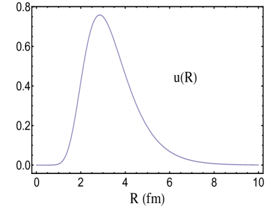
The radial solution to Eq. (II.1) is shown in the top panel in Fig. 1. The ensuing wavefunction reproduces the correct binding energy and charge radius of Helium-4. It also describes fairly well the empirical charge form factor of Helium-4 up-to momentum of the order of half the nucleon mass He and Zahed (2024a).
II.2 Argonne variational method
To include the D-wave contribution and more realistic nucleon pair interactions in Helium-4, we will make use of the Argonne symmetrized () variational wavefunction Lomnitz-Adler and Pandharipande (1980); Lomnitz-Adler et al. (1981); Wiringa (1991)
| (9) |
with the Jastrow trial state
where is a central pair correlation function, and the antisymmetric spin-isospin wavefunction in Eq. (4). The pair correlation functions built in the variational state, is valued in the set of operators making up the Argonne potential
| (10) |
with making up the 14 spin-isospin pair operators in the potential Lomnitz-Adler and Pandharipande (1980); Lomnitz-Adler et al. (1981); Wiringa (1991)
| (11) | |||||
Numerically the trial functions will turn out to be small, which allows us to simplify Eq. (9)
| (12) |
Using the spin-isospin identities Lomnitz-Adler and Pandharipande (1980)
| (13) |
To include the central three body correlation, the pair correlation function can be modified as follows Lomnitz-Adler and Pandharipande (1980); Lomnitz-Adler et al. (1981); Wiringa (1991).
| (14) |
where is chosen to be Wiringa (1991)
| (15) | |||||
we can rewrite Eq. (12) in the form
| (16) |
The Jastrow pair correlation function and the operator correlation functions , can be repacked in Eq. (II.2), in terms of their contributions to the singlet and triplet spin and isospin channels, using the identity Wiringa (1991); Lomnitz-Adler et al. (1981)
| (17) |
Here and are the spin and isospin projection operators, i.e.
| (18) |
The pair correlation functions , and can be related to the projected functions through
| (19) |
where we made use of Eq. (II.2). In the ground state of Helium-4 with , the spin-isospin projected functions and spin-singlet-tensor function can be obtained by solving the coupled Schrodinger equations Wiringa (1991)
| (20) |
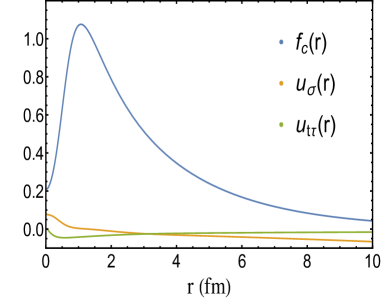
here refer to the explicit pair nucleon potentials. The eigenvalues include the screening effects at short distances, and their behavior at large distances is fixed by the asymptotic of the correlation functions. We refer to Wiringa et al. (1984); Wiringa (1991) for their explicit form. In Fig 1 we show our numerical results for , and , which are in overall agreement with those reported in Wiringa (1991). In appendix. A, we have tabulated our results for future comparison.
III Exchange currents in Helium-4
Helium-4 gravitational form factors in the impulse approximation were discussed in He and Zahed (2024a). In this section we extend the analysis to the exchange currents, following our recent discussion in the deuteron case He and Zahed (2024b). More specifically, the gravitational exchange contributions to Helium-4 in the single pion exchange approximation are illustrated in Fig. 2. We will refer to them generically by with the pair contribution (a), the seagull contribution (b), the pion exchange contribution (c) and the recoil corrections plus wavefunction renormalization (d). For a further assessment of the off-shellness effects between the pion-nucleon pseudoscalar and pseudovector couplings, we will discuss both, where we note that the seagull contribution (c) is absent for the former coupling. The explicit operator forms for each of these contributions are quoted in section IV below.
III.1 Matrix element: K-harmonic method
The generic structure of the matrix element in the K-harmonic method, can be recast into a multi-dimensional integral over the Jacobi coordinates
with the momentum of exchanged pion in Fig. 2. The argument of the Fourier transform refers to the struck nucleon relative to the center of mass coordinate, i.e.
| (22) |
is short for the inserted EMT operators in Fig. 2. Their explicit non-relativistic forms are listed in Eqs. (27), (33), (36) and (39) for the pair contribution, the seagull contribution, the pion exchange contribution and recoil contribution, respectively. To keep the hyperspherical symmetric, the Jacobi coordinates are set to be
The above integral can be reduced after integrating over the angular
| (24) | |||||

III.2 Matrix element: potential
The generic form of the exchange corrections, using the Argonne potential with the variational wave function (II.2) are of the form
| (25) | |||||
where . Here enforces the wavefunction normalization
| (26) |
Note that we have switched back to initial coordinates , and as integration variables, which tie to the Jacobi coordinates (II.1) by translational invariance, modulo a constant Jacobian. The latter can be eliminated in the ratio (25). To evaluate the multi-dimensional integral in Eq. (25), we will use the Monte Carlo method described in Lomnitz-Adler et al. (1981); Wiringa (1991).
IV Matrix element of EMT in Helium-4
To extract the non-relativistic contributions to the exchange currents, we will make use of the diagrams in Fig. 2, with the positive nucleon contribution in (a) subtracted, and the recoil contribution and wavefunction renormalization in (d) retained. The wiggly line refers to the insertion of the EMT, and the dashed line to the pion exchange contribution using both pseudo-vector coupling and pseudo-scalar coupling. Again, the explicit operator form for the EMT insertion for nucleon pairs in the context of the impulse approximation, is given in He and Zahed (2024a) and to which we refer for completeness. Instead, we will give the explicit integral expressions for the form factors for each contribution, using the K-Harmonic Method only. Those from the Argonne will be evaluated numerically using Eq. (25) by Monte Carlo sampling, with only the final results given in section V.
IV.1 Pair contribution
The EMT operator for the pair diagrams in Fig. 2a with pseudo-scalar coupling and pseudo-vector coupling, in the leading non-relativistic reduction read He and Zahed (2024b)
| (27a) | |||||
| (27b) | |||||
| (27c) | |||||
with the pion energy . The GFFs and for Helium-4 are related to the matrix elements of and through
Note that the term including breaks down the conservation law . As noted in He and Zahed (2024b), all contributions in Fig .2 need to be summed up, to uphold the conservation law. In particular, the contributions will be cancelled out. Therefore, we will not keep such a contribution in our following calculation. With this in mind, the corresponding GFFs for the pair diagrams with PS and PV coupling can be expressed as
| (29a) | |||||
| (29b) | |||||
| (29c) | |||||
where is the reduced hyper-radius wavefunction in Eq. (II.1), and factor is defined as
| (30) |
with the shorthand Yukawa potentials,
| (31) |
In the Helium-4 ground state, we can use Eq. (4) to obtain
| (32) |
IV.2 Seagull contribution
For the Seagull in Fig .2(b), the EMT operator can be written as He and Zahed (2024b)
| (33a) | |||||
| (33b) | |||||
There is no contribution from the seagull diagram for the PS coupling case. Also the contribution to from the PV coupling is equivalent to the contribution to from the pair diagram for the PS coupling,with the exception of the extra nucleon GFF A(k) in Eq. (27b). The GFFs can be obtained using the following relations
| (34) |
where
| (35a) | |||||
| (35b) | |||||
| (35c) | |||||
IV.3 Pion exchange contribution
The EMT exchange contributions stemming from the one-pion exchange in the non-relativistic reduction, are equivalent whether we use the PS or PV couplings. More specifically, the pertinent operators are He and Zahed (2024b)
| (36a) | |||||
| (36b) | |||||
with the identical matrix elements
| (37) |
where
| (38a) | |||||
| (38b) | |||||
| Here and the shorthand Yukawa potentials are expressed as | |||||
| (38c) | |||||
IV.4 Recoil contribution
The exchange operators stemming from the recoil terms after non-relativistic reduction are also equivalent whether we use the PS or PV coupling, they can be expressed as He and Zahed (2024b)
| (39a) | |||||
| (39b) | |||||
with the corresponding matrix elements
| (40) |
and
| (41) | |||||
V Numerical results
To summarise, the EMT exchange contributions to Helium-4 for the PS and PV pion nucleon couplings are given by
| (42) |
The main difference between the PS and PV couplings, is the additional contribution from the pair diagram to the component in the PS coupling case. A similar addition is noted in the charge form factor as in (B). We also note that the pair diagram contribution following from the PS coupling to , is very similar to that of the seagull diagram (absent for the PS coupling) with PV coupling. The only difference is the extra nucleon form factor included in (27b) in comparison to (33b).
The corresponding GFFs from the exchange currents are
| (43) |
To assess the pion GFFs in the pion exchange current contribution, we borrow their parameterization from the recent Lattice calculation in Hackett et al. (2023a),
| (44) |
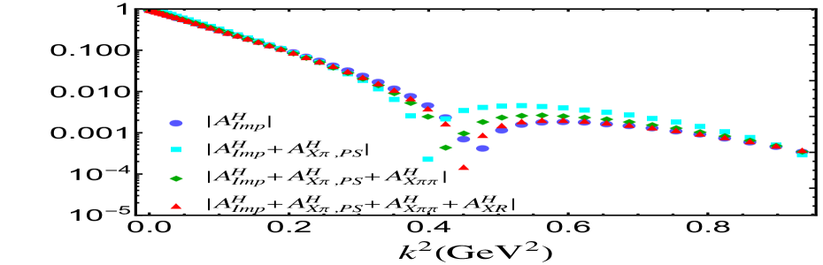
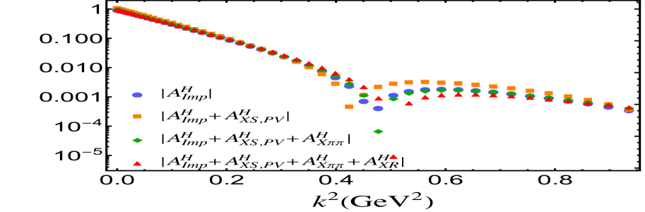
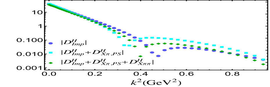
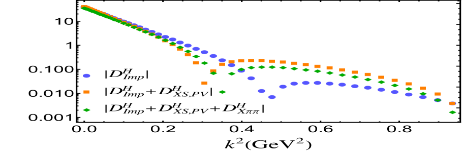
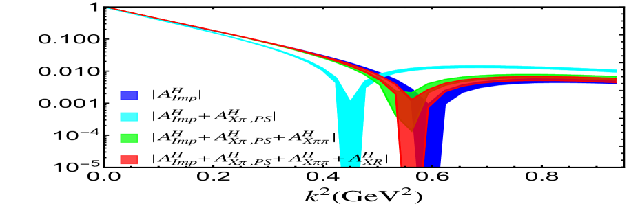
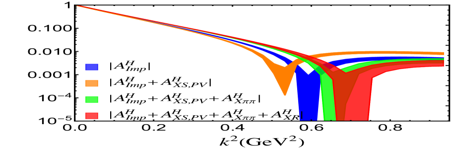
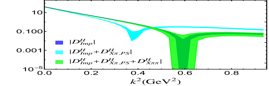
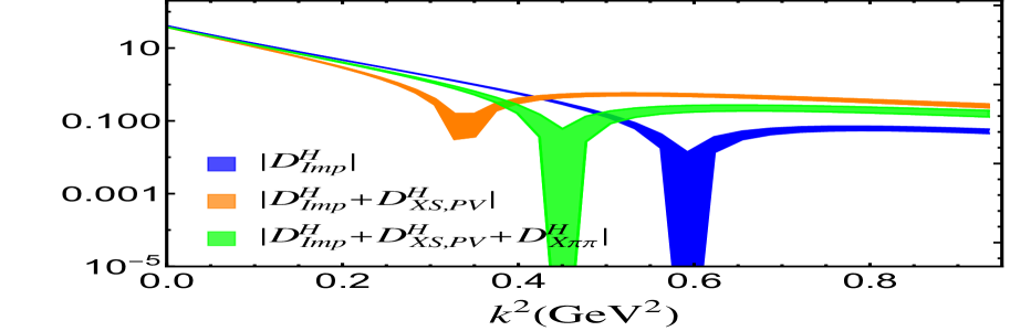
In Fig. 3 we show the Helium-4 GFFs using the pion-nucleon PS coupling (left) and the pion-nucleon PV coupling (right) with the K-Harmonic method. The results from the impulse approximation (blue-dots) are labeled by "" are from He and Zahed (2024a). The various contributions labeled by “", “", “", “" stem from the exchange contributions illustrated in Fig. 2a for the pair contribution, in Fig. 2b for the seagull contribution, in Fig. 2c for the pi-pi contribution and in Fig. 2d for the recoil contribution, respectively. The total corrections from the exchange currents using the PS coupling (red-triangle), do not yield qualitative changes to the GFFs from the impulse approximation (blue-dot). However, the contribution of the exchange currents with PV coupling yield lowe results compared to the impulse approximation. The difference is due to the pair contribution in Fig. 2a, whose contribution is higher order in the PV coupling. The contributions of the exchange currents to are comparable in the PS and PV case, since the only difference is the extra nucleon form factor included in , but absent in . Both shift the diffractive minima to the left of the impulse approximation.
In Fig. 4 we show the Helium-4 GFFs using the pion-nucleon PS coupling (left) and the pion-nucleon PV coupling (right) with the Argonne potential. The statistical uncertainties following from the Monte-Carlo sampling, are reflected in the colored-spreads when the various exchange contributions are added to the impulse approximation labeled by "" (blue-spread) results. Again, different contributions labeled by “", “", “", “" stem from the exchange contributions for the pair contribution, the seagull contribution, the pi-pi contribution and the recoil contribution, respectively. Unlike the K-harmonic method, the use of the Argonne potential with D-wave admixture, shows sensitivity to the use of the PS (left) versus PV (right) pion-nucleon coupling. The use of the PS coupling (left) shows that the additional contributions stemming from the exchange contributions when added up (read-spread), contribute net GFFS that are comparable with the impulse approximation (blue-spread) within statistics. This is not the case when using the PV coupling for the Helium-4 GFFs (right), with the net result of form factor (red band) is lower than result with impulse approximation (blue-spread), the diffractive minima of form factor (green-spread) is shifted to the left in comparison to that for impulse approximation (blue-spread). Again, the difference of form factor stems primarily from the component of pair diagram in the PS coupling. The difference in is caused by the extra nucleon GFF A(k) in (27b) with the PS coupling, when compared to (33b) with PV coupling. In both cases, the GFF diffractive minima from the impulse approximation, shift rightward in comparison to the K-harmonic method.
| r(fm) | |||
|---|---|---|---|
| 0.05 | 0.1644 | 0.2291 | 0 |
| 0.25 | 0.2626 | 0.3448 | 0.0339 |
| 0.50 | 0.5690 | 0.6491 | 0.0859 |
| 0.75 | 0.9069 | 0.9480 | 0.1264 |
| 1.00 | 1.0586 | 1.0735 | 0.1361 |
| 1.25 | 1.0512 | 1.0525 | 0.1255 |
| 1.50 | 0.9812 | 0.9694 | 0.1084 |
| 1.75 | 0.8965 | 0.8719 | 0.0916 |
| 2.00 | 0.8135 | 0.7783 | 0.0770 |
| 2.25 | 0.7369 | 0.6942 | 0.0650 |
| 2.50 | 0.6677 | 0.6203 | 0.0550 |
| 2.75 | 0.6056 | 0.5560 | 0.0469 |
| 3.00 | 0.5500 | 0.4999 | 0.0403 |
| 3.25 | 0.5002 | 0.4508 | 0.0349 |
| 3.50 | 0.4555 | 0.4077 | 0.0305 |
| 3.75 | 0.4153 | 0.3694 | 0.0268 |
| 4.00 | 0.3791 | 0.3354 | 0.0238 |
| 4.25 | 0.3464 | 0.3049 | 0.0212 |
| 4.50 | 0.3168 | 0.2775 | 0.0189 |
| 4.75 | 0.2900 | 0.2528 | 0.0169 |
| 5.00 | 0.2657 | 0.2305 | 0.0151 |
| 5.25 | 0.2436 | 0.2103 | 0.0136 |
| 5.50 | 0.2235 | 0.1920 | 0.0122 |
| 5.75 | 0.2052 | 0.1754 | 0.0109 |
| 6.00 | 0.1885 | 0.1603 | 0.0099 |
| 6.25 | 0.1733 | 0.1466 | 0.0089 |
| 6.50 | 0.1593 | 0.1341 | 0.0080 |
| 6.75 | 0.1466 | 0.1227 | 0.0072 |
| 7.00 | 0.1349 | 0.1123 | 0.0065 |
| 7.25 | 0.1242 | 0.1029 | 0.0059 |
| 7.50 | 0.1144 | 0.0943 | 0.0054 |
| 7.75 | 0.1054 | 0.0864 | 0.0049 |
| 8.00 | 0.0972 | 0.0792 | 0.0044 |
| 8.25 | 0.0896 | 0.0726 | 0.0040 |
| 8.50 | 0.0826 | 0.0666 | 0.0036 |
| 8.75 | 0.0762 | 0.0611 | 0.0033 |
| 9.00 | 0.0704 | 0.0561 | 0.0030 |
| 9.25 | 0.0650 | 0.0515 | 0.0027 |
| 9.50 | 0.0600 | 0.0472 | 0.0025 |
| 9.75 | 0.0554 | 0.0434 | 0.0023 |
| 10.00 | 0.0512 | 0.0388 | 0.0020 |
VI Conclusions
We have analyzed the exchange contributions to the GFFs for Helium-4. For that, we used a wavefunction that is maximally symmetric in the hyper-radius following from the K-harmonic method, with no D-wave admixture for simplicity. The results for the form factor are overall consistent with the one we recently reported using the impulse approximation in He and Zahed (2024a), whether we use the pion-nucleon PS or PV couplings. The diffractive minima of the form factor shift leftward when the exchange currents are added.
For comparison, we have also used a more realistic wavefunction following from the Argonne potential, with D-wave admixture. This approach is numerically intensive, and relies on Monte-Carlo sampling to generate the GFFs, with inherent statistical uncertainties that can be improved with longer runs. In this case, the exchange contributions were found to be overall consistent with the impulse approximation within statistics, when the pion-nucleon PS coupling is used. When the PV coupling is used, the exchange contributions are significant.
Our analysis of the charge form factor for Helium-4 carried for comparison in Appendix B. The exchange contributions from the PS coupling to the Helium-4 charge form factor, are larger in comparison to the impulse approximation when using the Argonne potential, significantly improving the agreement with experiment, while the PV coupling contributions are smaller and in agreement with the impulse approximation. For both cases, the diffractive GFF minima following from the impulse approximation, shift rightward in comparison to the K-harmonic result.
Overall, most of the exchange contributions are small in the range , leaving unchanged the mass radii. While they are separately sizable at higher momenta, fortunately their sum total is small, with the exception of the GFFs with PV coupling used with the Argonne potential. Since the Helium charge form factor is better described by the PS coupling using the Argonne potential, we expect the PS results for the GFFs with this potential to be more reliable.
The nucleon GFFs have been recently probed at JLab Ali et al. (2019); Duran et al. (2023), through near threshold photoproduction of charmonium. It would be useful to extend these experiments to Helium-4, for a better understanding of the role of the exchange currents in understanding the mass distribution in light nuclei, with a particular interest in extracting the pion GFF.
Acknowledgements
We thank Zein-Eddine Meziani and Robert Wiringa for discussions. FH is supported by the National Science Foundation under CAREER Award PHY- 1847893. IZ is supported by the Office of Science, U.S. Department of Energy under Contract No. DE-FG-88ER40388. This research is also supported in part within the framework of the Quark-Gluon Tomography (QGT) Topical Collaboration, under contract no. DE-SC0023646.
Appendix A Trial wave functions
In table 1, we list the numerical values of three wave-functions , , solution to the coupled Schrodinger equations (II.2) in the regime fm. In the regime fm, we use the asymptotic expressions in Wiringa (1991),
| (45) | |||||
Appendix B Electric form factor of Helium-4
In this appendix, we summarise the results for the charge form factor for Helium-4 using the K-Harmonic method, and the trial state using the Argonne potential. More specifically, the leading non-relativistic form for the isoscalar electric operators for the pair diagram with PS and PV couplings are
| (46) |
The operator for the recoil correction for both PS and PV is
| (47) | |||||
where and represent the iso-singlet combination of nucleon electric and magnetic form factors. The seagull diagram and pion exchange diagrams only contribute to the isospin vector form factor, not discussed here. The results of electric form factors can be easily obtained since the operator and are quite similar as and defined in Eq. (27a) and Eq. (39a).
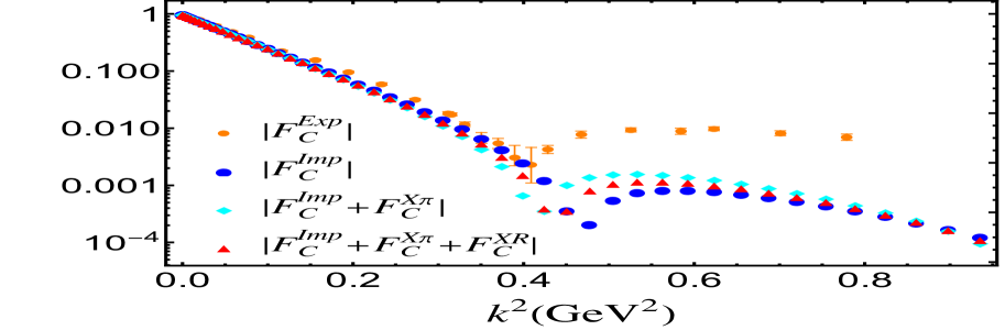
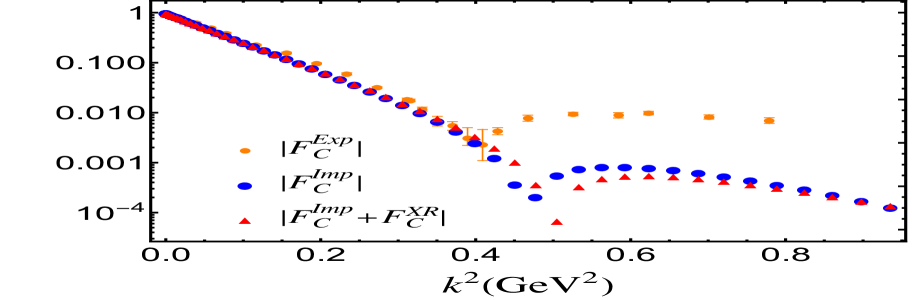
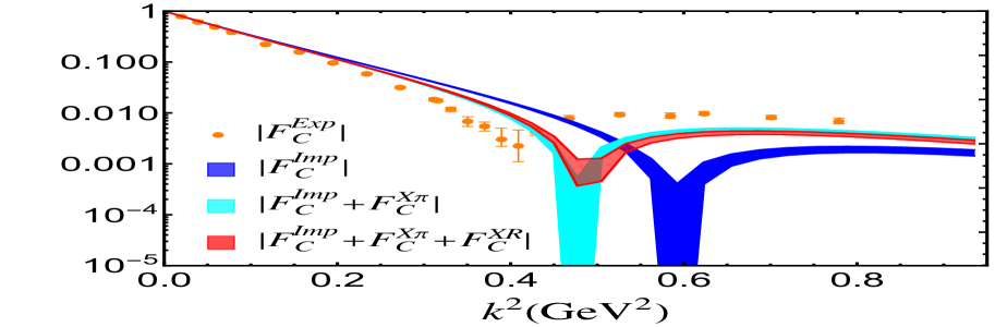
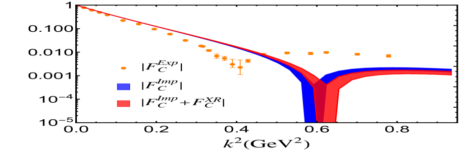
In Fig. 5 we show the results for Helium-4 charge form factor with the PS pion-nucleon coupling (left) and PV pion-nucleon coupling (right) using the K-Harmonics method with no D-wave admixture. The labels are “" (impulse approximation), “" (pair correction), “" (recoil correction) and “" (experiment) from Garcon et al. (1994). For comparison, we show in Fig. 6 the results of the Monte-Carlo simulation using the wavefunction generated from the Argonne potential with D-wave admixture, with the same labelings and color coding. The colored-spreads reflect on the statistical uncertainties. In the latter, the PS coupling yields a charge form factor that is in reasonable agreement with the data.
References
- Hackett et al. (2023a) Daniel C. Hackett, Patrick R. Oare, Dimitra A. Pefkou, and Phiala E. Shanahan, “Gravitational form factors of the pion from lattice QCD,” Phys. Rev. D 108, 114504 (2023a), arXiv:2307.11707 [hep-lat] .
- Hackett et al. (2023b) Daniel C. Hackett, Dimitra A. Pefkou, and Phiala E. Shanahan, “Gravitational form factors of the proton from lattice QCD,” (2023b), arXiv:2310.08484 [hep-lat] .
- Wang et al. (2024) Bigeng Wang, Fangcheng He, Gen Wang, Terrence Draper, Jian Liang, Keh-Fei Liu, and Yi-Bo Yang (QCD), “Trace anomaly form factors from lattice QCD,” Phys. Rev. D 109, 094504 (2024), arXiv:2401.05496 [hep-lat] .
- Polyakov and Schweitzer (2018) Maxim V. Polyakov and Peter Schweitzer, “Forces inside hadrons: pressure, surface tension, mechanical radius, and all that,” Int. J. Mod. Phys. A 33, 1830025 (2018), arXiv:1805.06596 [hep-ph] .
- Burkert et al. (2023) V. D. Burkert, L. Elouadrhiri, F. X. Girod, C. Lorcé, P. Schweitzer, and P. E. Shanahan, “Colloquium: Gravitational form factors of the proton,” Rev. Mod. Phys. 95, 041002 (2023), arXiv:2303.08347 [hep-ph] .
- Punjabi et al. (2015) V. Punjabi, C. F. Perdrisat, M. K. Jones, E. J. Brash, and C. E. Carlson, “The Structure of the Nucleon: Elastic Electromagnetic Form Factors,” Eur. Phys. J. A 51, 79 (2015), arXiv:1503.01452 [nucl-ex] .
- Ali et al. (2019) A. Ali et al. (GlueX), “First Measurement of Near-Threshold J/ Exclusive Photoproduction off the Proton,” Phys. Rev. Lett. 123, 072001 (2019), arXiv:1905.10811 [nucl-ex] .
- Duran et al. (2023) B. Duran et al., “Determining the gluonic gravitational form factors of the proton,” Nature 615, 813–816 (2023), arXiv:2207.05212 [nucl-ex] .
- Mamo and Zahed (2020) Kiminad A. Mamo and Ismail Zahed, “Diffractive photoproduction of and using holographic QCD: gravitational form factors and GPD of gluons in the proton,” Phys. Rev. D 101, 086003 (2020), arXiv:1910.04707 [hep-ph] .
- Guo et al. (2021) Yuxun Guo, Xiangdong Ji, and Yizhuang Liu, “QCD Analysis of Near-Threshold Photon-Proton Production of Heavy Quarkonium,” Phys. Rev. D 103, 096010 (2021), arXiv:2103.11506 [hep-ph] .
- Jo et al. (2015) H. S. Jo et al. (CLAS), “Cross sections for the exclusive photon electroproduction on the proton and Generalized Parton Distributions,” Phys. Rev. Lett. 115, 212003 (2015), arXiv:1504.02009 [hep-ex] .
- Abidin and Carlson (2009) Zainul Abidin and Carl E. Carlson, “Nucleon electromagnetic and gravitational form factors from holography,” Phys. Rev. D 79, 115003 (2009), arXiv:0903.4818 [hep-ph] .
- Belitsky and Ji (2002) Andrei V. Belitsky and X. Ji, “Chiral structure of nucleon gravitational form-factors,” Phys. Lett. B 538, 289–297 (2002), arXiv:hep-ph/0203276 .
- Polyakov and Sun (2019) Maxim V. Polyakov and Bao-Dong Sun, “Gravitational form factors of a spin one particle,” Phys. Rev. D 100, 036003 (2019), arXiv:1903.02738 [hep-ph] .
- Won et al. (2024) Ho-Yeon Won, Hyun-Chul Kim, and June-Young Kim, “Flavor structure of the energy-momentum tensor form factors of the proton,” Phys. Lett. B 850, 138489 (2024), arXiv:2302.02974 [hep-ph] .
- Hatta (2024) Yoshitaka Hatta, “Accessing the gravitational form factors of the nucleon and nuclei through a massive graviton,” Phys. Rev. D 109, L051502 (2024), arXiv:2311.14470 [hep-ph] .
- Lorcé (2024) Cédric Lorcé, “Electromagnetic and gravitational form factors of the nucleon,” in 25th International Spin Symposium (2024) arXiv:2402.00429 [hep-ph] .
- Mamo and Zahed (2022) Kiminad A. Mamo and Ismail Zahed, “J/ near threshold in holographic QCD: A and D gravitational form factors,” Phys. Rev. D 106, 086004 (2022), arXiv:2204.08857 [hep-ph] .
- Broniowski and Arriola (2008) Wojciech Broniowski and Enrique Ruiz Arriola, “Gravitational and higher-order form factors of the pion in chiral quark models,” Physical Review D 78 (2008), 10.1103/physrevd.78.094011.
- Frederico et al. (2009) T. Frederico, E. Pace, B. Pasquini, and G. Salmè, “Pion generalized parton distributions with covariant and light-front constituent quark models,” Physical Review D 80 (2009), 10.1103/physrevd.80.054021.
- Fanelli et al. (2016) Cristiano Fanelli, Emanuele Pace, Giovanni Romanelli, Giovanni Salmè, and Marco Salmistraro, “Pion generalized parton distributions within a fully covariant constituent quark model,” The European Physical Journal C 76 (2016), 10.1140/epjc/s10052-016-4101-1.
- Freese and Cloët (2019) Adam Freese and Ian C. Cloët, “Gravitational form factors of light mesons,” Physical Review C 100 (2019), 10.1103/physrevc.100.015201.
- Krutov and Troitsky (2021) A. F. Krutov and V. E. Troitsky, “Pion gravitational form factors in a relativistic theory of composite particles,” Phys. Rev. D 103, 014029 (2021), arXiv:2010.11640 [hep-ph] .
- Raya et al. (2022) Khepani Raya, Zhu-Fang Cui, Lei Chang, Jose-Manuel Morgado, Craig D. Roberts, and Jose Rodriguez-Quintero, “Revealing pion and kaon structure via generalised parton distributions *,” Chin. Phys. C 46, 013105 (2022), arXiv:2109.11686 [hep-ph] .
- Xu et al. (2024) Yin-Zhen Xu, Minghui Ding, Khépani Raya, Craig D. Roberts, José Rodríguez-Quintero, and Sebastian M. Schmidt, “Pion and kaon electromagnetic and gravitational form factors,” Eur. Phys. J. C 84, 191 (2024), arXiv:2311.14832 [hep-ph] .
- Li and Vary (2024) Yang Li and James P. Vary, “Stress inside the pion in holographic light-front qcd,” Physical Review D 109 (2024), 10.1103/physrevd.109.l051501.
- Broniowski and Ruiz Arriola (2024) Wojciech Broniowski and Enrique Ruiz Arriola, “Gravitational form factors of the pion and meson dominance,” (2024), arXiv:2405.07815 [hep-ph] .
- Liu et al. (2024a) Wei-Yang Liu, Edward Shuryak, and Ismail Zahed, “Gluon contributions to nucleon matrix elements in the QCD instanton vacuum,” To Appear (2024a).
- Liu et al. (2024b) Wei-Yang Liu, Edward Shuryak, Christian Weiss, and Ismail Zahed, “Pion gravitational form factors in the QCD instanton vacuum I,” (2024b), arXiv:2405.14026 [hep-ph] .
- Sick (2008) Ingo Sick, “Precise root-mean-square radius of He-4,” Phys. Rev. C 77, 041302 (2008).
- Riska (1989) Dan Olof Riska, “EXCHANGE CURRENTS,” Phys. Rept. 181, 207 (1989).
- Mibe et al. (2007) T. Mibe et al. (CLAS), “First measurement of coherent phi-meson photoproduction on deuteron at low energies,” Phys. Rev. C 76, 052202 (2007), arXiv:nucl-ex/0703013 .
- Chang et al. (2008) W. C. Chang et al., “Forward coherent phi-meson photoproduction from deuterons near threshold,” Phys. Lett. B 658, 209–215 (2008), arXiv:nucl-ex/0703034 .
- He and Zahed (2024a) Fangcheng He and Ismail Zahed, “Gravitational form factors of light nuclei: Impulse approximation,” Phys. Rev. C 109, 045209 (2024a), arXiv:2310.12315 [nucl-th] .
- Garcia Martin-Caro et al. (2023) Alberto Garcia Martin-Caro, Miguel Huidobro, and Yoshitaka Hatta, “Gravitational form factors of nuclei in the Skyrme model,” Phys. Rev. D 108, 034014 (2023), arXiv:2304.05994 [nucl-th] .
- Hockert et al. (1973) J. Hockert, D. O. Riska, M. Gari, and A. Huffman, “Meson exchange currents in deuteron electrodisintegration,” Nucl. Phys. A 217, 14–28 (1973).
- Chemtob et al. (1974) M. Chemtob, E. J. Moniz, and Mannque Rho, “Deuteron Electromagnetic Structure at Large Momentum Transfer,” Phys. Rev. C 10, 344–352 (1974).
- Kloet and Tjon (1974) W. M. Kloet and J. A. Tjon, “MESON EXCHANGE EFFECTS ON THE CHARGE FORM-FACTORS OF THE TRINUCLEON SYSTEM,” Phys. Lett. B 49, 419–422 (1974).
- Jackson et al. (1975) A. D. Jackson, A. Lande, and D. O. Riska, “Pion exchange currents in elastic electron deuteron scattering,” Phys. Lett. B 55, 23–27 (1975).
- Freese and Cosyn (2022) Adam Freese and Wim Cosyn, “Spatial densities of momentum and forces in spin-one hadrons,” Phys. Rev. D 106, 114013 (2022), arXiv:2207.10787 [hep-ph] .
- He and Zahed (2024b) Fangcheng He and Ismail Zahed, “Deuteron gravitational form factors: exchange currents,” (2024b), arXiv:2401.09318 [nucl-th] .
- Wiringa et al. (1984) Robert B. Wiringa, R. A. Smith, and T. L. Ainsworth, “Nucleon Nucleon Potentials with and Without Delta (1232) Degrees of Freedom,” Phys. Rev. C 29, 1207–1221 (1984).
- Castilho Alcaras and Pimentel Escobar (1974) J. Castilho Alcaras and B. Pimentel Escobar, “Application of the Basic Approxirnation of the K-Harmonics Method to the Alpha Particle,” Revista Brasileira de Física 4, 83 (1974).
- Wiringa (1991) Robert B. Wiringa, “Variational calculations of few-body nuclei,” Phys. Rev. C 43, 1585–1598 (1991).
- Lomnitz-Adler and Pandharipande (1980) J. Lomnitz-Adler and V. R. Pandharipande, “A simple and realistic triton wave function,” Nucl. Phys. A 342, 404–420 (1980).
- Lomnitz-Adler et al. (1981) J. Lomnitz-Adler, V. R. Pandharipande, and R. A. Smith, “Monte Carlo calculations of triton and 4 He nuclei with the Reid potential,” Nucl. Phys. A 361, 399–411 (1981).
- Garcon et al. (1994) M. Garcon et al., “Tensor polarization in elastic electron - deuteron scattering in the momentum transfer range 3.8-fm**-1 = q = 4.6-fm**-1,” Phys. Rev. C 49, 2516–2537 (1994).