Title

Optimal policy design for decision problems under social influence

Abstract

This paper focuses on devising strategies for control-oriented decision-making scenarios, in the presence of social and external influences, e.g. within recommending systems in social contexts. More precisely, we extend the classical Friedkin and Johnsen model of opinion dynamics to incorporate random factors, such as variability in individual predisposition, and uncertainty in social acceptance towards a specific action that a recommending system aims to promote. Furthermore, we formulate an optimization-based control problem aimed at fostering the social acceptance of particular actions within the network. Initially conceptualized as an economic cost minimization, in this preliminary work, we simplify our problem by reformulating it into an MPC framework. Through our analysis and numerical simulations, we illustrate the effectiveness of the proposed methodologies.

I Introduction

Individuals frequently take repeated decisions when it comes to their daily routines, such as selecting their mode of transportation for commuting or deciding whether or not to use certain services. In making these decisions, individuals are heavily influenced by both social environment and external factors [1]. However, individuals often exhibit resistance to change demonstrating stubborn behaviors that can derive from a limited predisposition towards specific actions, due to individual rational or psychological factors [2]. Indeed, services and technologies with considerable positive impacts on society and the environment often encounter doubt or resistance from potential users. Individuals are often hesitant to change their behavior and habits, even when it could benefit them in the long run. Therefore, policies that encourage specific virtuous action or the adoption of technological innovations in society are necessary. These policies should consider the complex relationships between individuals, their characteristics and connections, and the consequences of past policy decisions [3, 4].

Some recent works started investigating the influence of recommending systems on the dynamics within social networks. Specifically, building on the work in [5], where a feedback interaction between a recommending system and a single user is introduced, [6, 7] integrate the dynamics of social interactions and recommending system within influence networks. Notably, the paper [8] introduces a model-based control approach for user engagement maximization, based on a Model Predictive Control (MPC) strategy that takes into account the evolution of opinions.

In this paper, our goal is to develop new strategies tailored to effectively managing control mechanisms within repetitive decision-making scenarios. To achieve this goal, we propose a new model, based on the classical Friedkin and Johnsen model of opinion dynamics [2], a well-established opinion dynamics known for its ability to capture the intricate interplay between individual behaviors and social influences. Specifically, we extend this model by incorporating random factors such as a variability of predisposition and the random nature of social acceptance towards specific actions that recommending systems seek to promote. In the absence of external control action, this dynamics does not converge but persistently oscillates. However, under suitable assumptions, it can be proved that the resulting stochastic process converges almost surely to a final limit and the system is ergodic, meaning that, over a sufficiently long period, the time averages of inclinations converge to their expected values.

With this in mind, we address the aforementioned decision-making problem by formulating an optimization-based control framework designed to foster the propagation and acceptance of desired actions within the network. Compared to [8], the policy maker is not intended as a new node introduced in the network, able to influence at each time individuals with an equal action, but is intended as a personalized external influence. Furthermore, unlike prior literature, our model-based approach does not entail observing opinions reflecting inclinations toward acceptance. Instead, we are restricted to observing only their realizations. Initially conceived as an economic cost, our approach is based on two possible approximations, leading to quadratic losses and, hence, making our problem tractable within a model predictive control (MPC) framework. This strategic reformulation not only enhances the robustness of our approach but also significantly amplifies its efficacy in achieving desired outcomes within dynamic social environments, allowing us to design meaningful policy actions.

The paper is structured as follows. Section II introduces the proposed model for opinion dynamics along with its open-loop properties. Section III shifts to a closed-loop setting, introducing a suite of approximated policy design strategies, which intend to nudge individuals toward positive biases. The impact of these policies is analyzed in Section IV by a numerical example. The paper is then concluded with some remarks and directions for future work.

II Model & Open-loop analysis

We consider a social network represented by a directed graph $\mathcal{G}=(\mathcal{V,E},\bm{P})$ that is constituted by a collection of nodes $v\in\mathcal{V}$ or agents and edges $\mathcal{E}$ describing the interactions among them. The interpersonal influence among the agents is encoded in a weight matrix $\bm{P}$. More precisely, $\bm{P}$ is adapted to the graph, i.e. $P_{v,w}\neq 0\iff(v,w)\in\mathcal{E}$. If $(v,w)\in\mathcal{E}$ we say that $v$ follows $w$ or is influenced by $w$. We denote the set of agents followed by $v$ with the set $\mathcal{N}_{v}=\{w\in\mathcal{V}:P_{vw}>0\}$. We assume that $\bm{P}$ is a stochastic nonnegative matrix, i.e., $\sum_{w\in\mathcal{V}}P_{vw}=1$ for all $v\in\cal{V}$. Each agent is endowed with a state that represents the latent opinion/belief at time $t$ about a specific decision. Without loss of generality, we assume that $x_{i}(0)\in[0,1],\ \forall i\in\mathcal{V}$ where an opinion close to $0$ indicates opposition, while an opinion close to $1$ indicates support for it. At each time step $t\in\mathbb{Z}_{\geq 0}$ the opinion of an agent $v\in\mathcal{V}$ is updated as a response to the interaction with the neighbors, according to the following rule

$$x_{v}(t+1)=\lambda_{v}P_{vv}x_{v}(t)+\lambda_{v}\!\!\!\!\!\!\!\!\sum_{w\in\mathcal{N}_{v}\setminus\{v\}}\!\!\!\!\!\!P_{vw}y_{w}(t)\!+\!(1\!-\lambda_{v})u_{v}(t),$$ (1)

where $\lambda_{v}\in[0,1]$ is the relative weight of social influence. Note that this dynamic is steered not only by social influences (as already proposed in [2]), but also by an “input” $u_{v}(t)$, here dictated by

$$u_{v}(t)=\underbrace{u_{\mathrm{o}}+u_{v}^{c}(t)}_{:=\bm{\tilde{u}}(t)}+u_{v}^{nc}(t),~{}~{}u_{v}(t)\in[0,1],$$ (2)

where $u_{0}\in[0,1]$ indicates the individual bias of the agent, which steers its opinion along with the social influence in the absence of policy influences, a deterministic input $u_{v}^{c}(t)\in[0,1-{u}_{0}]$ that a policy maker can shape (i.e., through incentive strategies, information campaigns etc.) to nudge a change in the individual inclination and an uncontrollable input $u_{v}^{nc}(t)\in\Phi\subseteq[0,1]$ representing possible (yet unpredictable) variations in individual opinions due to external factors (e.g., changes in the weather and, thus, the choice not to take a shared bike). Due to its unpredictability, we here assume $u_{v}^{nc}(t)$ to be a zero-mean, white sequence uniformly distributed in the interval $[-\delta\bm{u}_{\mathrm{o}},\delta\bm{u}_{\mathrm{o}}]$, with $0<\delta\ll 1$. This assumption implies that the changes induced by these external factors cannot overcome the prior individual bias $\bm{u}_{\mathrm{o}}$, but only cause slight changes in the individual opinion.

By defining the vector $\bm{x}(t)\in\mathbb{R}^{|\mathcal{V}|}$ grouping the inclinations of all agents in the network, the vector $\bm{y}(t)\in\mathbb{R}^{|\mathcal{V}|}$ collecting all the measured opinions and the vector $\bm{u}(t)\in\mathbb{R}^{|\mathcal{V}|}$ of all inputs, the previous dynamics can be written in matrix form as

$$\bm{x}(t+1)=[\bm{\lambda}](\bm{P}-[\bm{P}])\bm{y}(t)+[\bm{\lambda}][\bm{P}]\bm{x}(t)+(\bm{I}-[\bm{\lambda}])\bm{u}(t),$$ (3)

where $[\bm{P}]$ denotes a diagonal matrix with elements equal (and equally ordered) to those in the diagonal of $\bm{P}$ and $[\bm{\lambda}]$ stems for a diagonal matrix with diagonal entries equal to $\bm{\lambda}$. From now on we will make the following assumption on the topology of the influence network associated with $\bm{P}$.

Assumption 1 (Network topology).

We assume that, for any node $v\in\mathcal{V}$, there exists a path from $v\in\mathcal{V}$ to a node $s\in\mathcal{V}$ such that $\lambda_{s}<1$.

Assumption 2 (Acceptance variables).

Given the initial condition $x_{v}(0)\in[0,1]$ for $t\in\mathbb{N},$ we assume that the acceptance variables are random variables with the conditional distribution given by

$$\mathbb{P}(y_{v}(t)=1|\bm{x}(t))=x_{v}(t),$$

$$\mathbb{P}(y_{v}(t)=0|\bm{x}(t))=1-x_{v}(t).$$

Remark 1 (Heterogeneous updates).

In the model all agents update its state at each discrete time-step and the randomness is introduced exclusively from the fact that agents react in a random manner based on the latent opinion. In more realistic scenarios, the individuals can interact in a random manner and the activation rate among individuals can be heterogenous. We remark that this random behavior can be included easily in the weight matrix $\bm{P}$.

The presence of uncertainty in the acceptance makes the system unstable and both the latent and acceptance variables continue to oscillate.

II-A Asymptotic behavior with absence of control

Without any control, i.e. if $\bm{u}^{\mathrm{c}}(t)=0$ for all $t\in\mathbb{N}$, as a consequence of Eq. (1), the evolution of expected dynamics converges to a final limit profile. The limit behavior of the opinions is described in the following result.

Proposition 1 (Expected dynamics).

Under Assumption 1 and Assumption 2, for every initial condition $\bm{x}(0)\in\mathbb{R}^{\mathcal{V}}\in[0,1]$, the dynamics in (1) is such that

$$\mathbb{E}[\bm{x}(t+1)]=[\bm{\lambda}]\bm{P}\mathbb{E}[\bm{x}(t)]+(\bm{I}-[\bm{\lambda}])\bm{u}_{0}$$

for any $t\in\mathcal{N}$ and

$$\mathbb{E}[{\bm{x}}(\infty)]=(I-[\bm{\lambda}]\bm{P})^{-1}(I-[\bm{\lambda}])\bm{u}_{0}.$$ (4)

In particular, the social system is stable and a final opinion limit profile emerges that is a combination of the exogenous inputs. The proof is straightforward using standard techniques devised in modeling and analysis of dynamic social networks [9] and we omit the details.

Definition 1 (Ergodic process).

If there exists a random variable $\bm{x}_{\infty}\in^{\mathcal{V}}$ such that almost surely

$$\lim_{k\to\infty}\frac{1}{k}\sum_{\ell=0}^{k-1}\bm{x}({\ell})=\mathbb{E}[\bm{x}_{\infty}],$$ (5)

then the process $\{\bm{x}(k)\}_{k\in\mathbb{Z}_{\geq 0}}$ will be said ergodic. The time-average in Eq. (5) is called Cesáro average.

We now summarize a simple result about the dynamics: its proof is a straightforward application of techniques in [10].

Theorem 1 (Ergodicity).

Consider the random processes $\{\bm{x}(k)\}_{k\in\mathbb{Z}_{\geq 0}}$ defined in (1) and $\{\bm{y}(k)\}_{k\in\mathbb{Z}_{\geq 0}}$, then

1. $\bm{x}(k),\bm{y}(k)$ converge in distribution to random variables $\bm{x}_{\infty},\bm{y}_{\infty}$, and the distribution of $\bm{x}_{\infty},\bm{y}_{\infty}$

2. the process is ergodic;

3. the limit random variables satisfy $\mathbb{E}[\bm{x}_{\infty}]=\mathbb{E}[\bm{y}_{\infty}]=\bm{x}^{\star}.$

In order to illustrate the behavior of the dynamics, we will consider the following example.

Example 1.

We consider a simple network consisting of $n=20$ nodes. The topology is a realization of an Erdös Renyi graph with connection probability $p=0.2$. For simplicity, the weights of the networks are uniform for all $v$ and $w\in\mathcal{V}$. The initial conditions $y_{v}(0)$ are i.i.d. Bernoulli with parameter $1/2$. For $t\in\mathcal{N}$ the expressed opinions are random variables with the conditional distribution $\mathbb{P}(\bm{y}(t)=1|\bm{x}(t))=\bm{x}(t)$ In Figure 1 the latent opinions and acceptance realizations are shown as a function of times. The latent opinions oscillate in the range $[0,1]$ and produce the acceptance realizations.

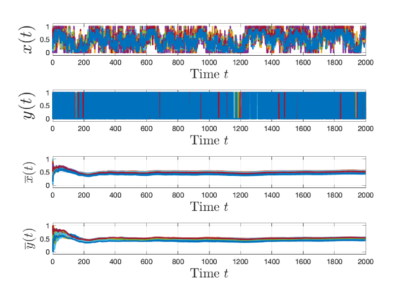
Figure 1: Opinion dynamics in a simple network.

III Optimal design of policy interventions

As the input dictating sudden changes in individual opinion is assumed to be unpredictable, for now, we rely on the mean dynamics of design policy actions to nudge the agents.

Our goal is to steer individual opinions (at least on average) toward the acceptance of the innovation, which we can translate into the following cost

$$J_{\infty}:=\sum_{t=0}^{+\infty}\mathbb{E}[\|\bm{1}-\bm{y}(t)\|_{2}^{2}]+r\|\bm{u}^{c}(t)\|_{2}^{2},$$ (6)

where $\bm{u}^{c}(t)\in[0,1-\bm{u}_{0}]$ collects only the controllable part of the input and $r>0$ controls the relative importance of achieving adoption across the network and keeping the policy effort at the minimum level. Note that the cost function in Eq. (6) can be rewritten as an economic cost function as detailed in the following proposition.

Proposition 2.

The cost function in Eq. (6) can be rewritten as follows

$$J_{\infty}=\sum_{t=0}^{+\infty}\|\bm{1}-\mathbb{E}[\bm{x}(t)]\|_{1}+r\|\bm{u}^{c}(t)\|_{2}^{2}.$$ (7)

Proof.

We denote $\bm{\mu}(t)=\mathbb{E}[\bm{x}(t)]$. Now, let consider the fist term in the summation in Eq. (6). We have

$$\mathbb{E}[\|\bm{1}\!-\!\bm{y}(t)\|_{2}^{2}]=\mathbb{E}[\mathbb{E}[\|\bm{1}-\bm{y}(t)\|_{2}^{2}|\bm{x}(t)]].$$

Standard computations lead to the following series of equalities:

$$\mathbb{E}[\|\bm{1}-\bm{y}(t)\|_{2}^{2}|\bm{x}(t)]\!$$

$$\quad=\!\|\bm{1}\!-\!\mathbb{E}[\bm{y}(t)|\bm{x}(t)]\|_{2}^{2}\!+\!\mathbb{E}[\|\bm{y}(t)\!-\!\mathbb{E}[\bm{y}(t)|\bm{x}(t)]\|_{2}^{2}]$$ (8)

$$\quad=\|\bm{1}-\bm{x}(t)\|_{2}^{2}\!+\!\mathbb{E}\left[\|\bm{y}(t)-\bm{x}(t)\|_{2}^{2}|\bm{x}(t)\right]$$

$$\quad=\|\bm{1}\!-\!\bm{x}(t)\|_{2}^{2}+\!\sum_{v\in\mathcal{V}}\mathbb{E}[(y_{v}(t)\!-\!x_{v}(t))^{2}|\bm{x}(t)]$$

$$\quad=\|\bm{1}\!-\!\bm{x}(t)\|_{2}^{2}\!+\!\sum_{v\in\mathcal{V}}x_{v}(t)(1\!-\!x_{v}(t))$$

$$\quad=\sum_{v\in V}(1\!-\!x_{v}(t))^{2}\!+\!\sum_{v\in\mathcal{V}}x_{v}(t)(1\!-\!x_{v}(t))$$

$$\quad=\sum_{v\in V}(1-x_{v}(t))$$ (9)

from which, by taking the expactation, we get

$$\mathbb{E}[\|\bm{1}\!-\!\bm{y}(t)\|_{2}^{2}]=\!\|\mathbf{1}\!-\!\mathbb{E}[\bm{x}(t)]\|_{1}.$$

By replacing this term in Eq. (6), we conclude the proof. ∎

From now on we will denote $\bm{\mu}(t)=\mathbb{E}[\bm{x}(t)]$ and, initially, we assume it to be directly measured.

III-A Conservative policy design

As a first strategy to handle the economic loss in Eq. (7), we replace it with its lower bound

$$\hat{J}_{\infty}=\sum_{t=0}^{+\infty}\|\mathbf{1}-\bm{\mu}(t)\|_{2}^{2}+r\|\bm{u}^{c}(t)\|_{2}^{2},$$ (10)

hence shifting to a “simpler”, yet conservative quadratic loss. This cost does not yet represent something that a practical policy can minimize, since actual policies will never be enacted for an infinite period of time (as they should be reconsidered based on technological advances etc.). Therefore, we further shift from an infinite-horizon cost to a finite-horizon one. This choice allows us to formulate the following model predictive control (MPC) problem on the mean opinion dynamics:

$$\min_{\tilde{U}}\hat{J}_{T}(\tilde{U})$$ (11)

$$\mbox{s.t. }~{}\tilde{\bm{\mu}}(k+1)=[\bm{\lambda}]\bm{P}\tilde{\bm{\mu}}(k)+(\bm{I}-[\bm{\lambda}])(\bm{u}_{0}+\tilde{\bm{u}}^{c}(k)),$$

$$\qquad\tilde{\bm{u}}^{c}(k)\in[0,\mathbf{1}-\bm{u}_{0}],~{}~{}~{}\forall k\in[0,T-1],$$

$$\qquad\tilde{\bm{\mu}}(0)=\bm{\mu}(t),$$

$$\qquad\|\mathbf{1}-\tilde{\bm{\mu}}(k+1)\|_{1}\leq\alpha\|\mathbf{1}-\tilde{\bm{\mu}}(k)\|_{1},~{}k\!\in\![0,T\!-1],$$

where $\tilde{U}=\{\tilde{\bm{u}}^{c}(k)\}_{k=0}^{T-1}$, $T\geq 1$ is the chosen policy design horizon, the loss is given by

$$\hat{J}_{T}(\tilde{U})=\sum_{k=0}^{T-1}\|\mathbf{1}-\tilde{\bm{\mu}}(k)\|_{2}^{2}+r\|\tilde{\bm{u}}^{c}(k)\|_{2}^{2},$$ (12)

and, for $\alpha<1$, the last is a contraction constraint enforcing the predictive tracking error to reduce at each time instant (similar to the one proposed in [11]). This problem should be solved in a receding-horizon fashion at each policy design step $t\in\mathbb{N}$, keeping track and, hence, adapting to changes in the mean inclination of agents with respect to the new technology.

Even if appealing, this formulation still neglects one of the factors that affect individual opinions, i.e., the impact of uncontrollable disturbances $\bm{u}^{nc}(t)$. However, not accounting for its effect might lead to policies that do not guarantee $\bm{\mu}(t)\in[0,1]^{N}$, ultimately making the scheme in Eq. (11) not recursively feasible. Given our modelling assumptions (see Section II), we thus frame a worst-case policy design problem as follows

$$\min_{\tilde{U}}\hat{J}_{T}(\tilde{U})$$ (13)

$$\mbox{s.t. }~{}\tilde{\bm{\mu}}(k+1)=[\bm{\lambda}]\bm{P}\tilde{\bm{\mu}}(k)+(\bm{I}-[\bm{\lambda}])(\bm{u}_{0}+\tilde{\bm{u}}^{c}(k)),$$

$$\qquad\tilde{\bm{u}}^{c}(k)\in[\bm{0},\mathbf{1}-\bm{u}_{0}^{\prime}],~{}~{}~{}\forall k\in[0,T-1],$$

$$\qquad\tilde{\bm{\mu}}(0)=\bm{\mu}(t),$$

$$\qquad\|\mathbf{1}-\tilde{\bm{\mu}}(k+1)\|_{1}\leq\alpha\|\mathbf{1}-\tilde{\bm{\mu}}(k)\|_{1},~{}~{}k\in[0,T-1],$$

where $J_{T}(\tilde{U})$ is still defined as in Eq. (12), while we have included the (worst case) effect of input disturbances by replacing $\bm{u}_{0}$ with $\bm{u}_{0}^{\prime}=\bm{u}_{0}+\sqrt{\frac{(\delta\bm{u}_{0})^{2}}{3}}$ (i.e., the mean summed to the standard deviation of the uniformly distributed noise) in the input constraints.

III-B An alternative loss to track opinion shifts

Whenever the $\mu(t)$ converges (i.e., $|\mu(t+1)-\mu(t)|\rightarrow 0$), then the 1-norm characterizing the economic loss in Eq. (6) can be approximated as

$$\|1-\bm{\mu}(t)\|_{1}\rightarrow\sum_{v\in V}\frac{\|\bm{1}-\bm{\mu}_{v}(t)\|_{2}^{2}}{|\bm{1}-\bm{\mu}_{v}(t-1)|}.$$ (14)

By relying on this intuition, the initial cost in Eq. (7) can hence be approximated with

$$\tilde{J}_{\infty}=\sum_{t=0}^{+\infty}\|\bm{1}-\bm{\mu}(t)\|^{2}_{Q(\bm{\mu}(t))}+r\|\bm{u}^{c}(t)\|_{2}^{2},$$ (15)

where $Q(\bm{\mu}(t))$ is a diagonal matrix, with

$$Q_{v}(\mu_{v}(t))=\left(|1-\mu_{v}(t-1)|\right)^{-1},$$ (16)

for all $t\geq 0$ and for all $v\in\mathcal{V}$.

In turn, when shifting to a finite-horizon setting, this alternative approximation leads to the following policy design problem:

$$\min_{\tilde{U}}\tilde{J}_{T}(\tilde{U})$$ (17)

$$\mbox{s.t. }~{}\tilde{\bm{\mu}}(k+1)=[\bm{\lambda}]P\tilde{\bm{\mu}}(k)+(I-[\bm{\lambda}])(\bm{u}_{0}^{\prime}+\tilde{\bm{u}}^{c}(k)),$$

$$\qquad\tilde{\bm{u}}^{c}(k)\in[\bm{0},\mathbf{1}-\bm{u}_{0}^{\prime}],~{}~{}~{}\forall k\in[0,T-1],$$

$$\qquad\tilde{\bm{\mu}}(0)=\bm{\mu}(t),$$

$$\qquad\|\mathbf{1}-\tilde{\bm{\mu}}(k+1)\|_{1}\leq\alpha\|\mathbf{1}-\tilde{\bm{\mu}}(k)\|_{1},~{}~{}k\in[0,T-1],$$

where

$$\tilde{J}_{T}(\tilde{U})= \sum_{k=0}^{T-1}\|\mathbf{1}-\tilde{\bm{\mu}}(k)\|_{Q(\bm{\mu}(t+k))}^{2}+r\|\tilde{\bm{u}}^{c}(k)\|_{2}^{2}$$

$$+\|\mathbf{1}-\tilde{\bm{\mu}}(T)\|_{Q(\bm{\mu}(t+T))}^{2}.$$ (18)

Note that this design choice requires adjusting the penalties in the control cost over time. This allows us to progressively recover the finite-horizon counterpart of the original economic cost if the input and the mean dynamics converge to a steady state. Indeed, if such a condition is verified, $\bm{u}(t)\rightarrow\bar{\bm{u}}$ and, consequently, $\bm{\mu}(t)\rightarrow\bar{\bm{\mu}}$. In turn, by continuity of the norm $\|\bm{1}-\bar{\bm{\mu}}(t)\|^{2}_{Q(\bm{\mu}(t))}\rightarrow\|\bm{1}-\bar{\bm{\mu}}\|^{2}_{Q(\bar{\bm{\mu}})}=\|\bm{1}-\bar{\bm{\mu}}\|_{1}$. Future work will be devoted to analyzing the conditions under which this result holds and, hence, understanding when solving Eq. (17) can be worthwhile.

Indeed, while in principle allowing the calibration of the impact of the tracking term in the cost (i.e., the first and last terms), including this time-varying weight makes the overall control problem more complex. In particular, it would require a preview on $\bm{\mu}(t+k)$, for $k=0,\ldots,T$. To circumvent this limitation, we propose the scheme summarized in the following steps.

At each time instant $t\geq 0$, we propose to do the following.

1. Exploit the optimal sequence computed at the previous instant $t$ to construct the “candidate” input sequence

   $$\bar{U}=\{\tilde{u}^{c,\star}(t|t-1),\ldots,\tilde{u}^{c,\star}(t+T-1|t-1),0\},$$

   which is feasible with our structural input constraints.

2. Use $\bar{U}$ to predict the evolution of the mean inclination $\{\mu^{p}(t+k)\}_{k=0}^{T-1}$ through our mean inclination model, i.e.,

   $$\mu^{p}(t+k+1)=[\lambda]P\mu^{p}(t+k)+(I-[\lambda])(u_{\mathrm{o}}+\bar{u}(k-1)),$$

   with $\bar{u}(k-1)$ being the $k-1$-th element of the sequence $\bar{U}$, for $k\in[0,T-1]$.

3. Approximate the original weights in Eq. (16) as

   $$\tilde{Q}_{v}(\mu_{v}^{p}(t+k))=\|1-\mu_{v}^{p}(t+k)\|^{-1}.$$ (19)

This procedure ultimately results in an alternative approximated solution to the policy design problem with cost Eq. (7).

III-C Policy design with estimated mean inclinations

The previous schemes still relied on the exact knowledge of $\bm{\mu}(t)$, which is not actually available to the policymaker. At the same time, under our assumptions, the policymaker can instead access the acceptance variables $\bm{y}(t)$ of individuals. The latter can be used to define a practical estimate of the mean inclination over time as

$$\hat{\bm{\mu}}(t)=\frac{1}{t}\sum_{\tau=0}^{t-1}\bm{y}(\tau).$$ (20)

Remark 2.

The main rationale behind employing this estimator is based on the assumption that if the ergodicity of the system is preserved under the control action then we expect that the Cesaro time-averages converge to their expected value, i.e. $\mathbb{E}[\|\widehat{\bm{\mu}}(t)-\bm{\mu}(t)\|_{2}^{2}]\rightarrow 0$.

We can hence recast the ideal problems in Eq. (11) and Eq. (17) as follows

$$\min_{\tilde{U}}J_{T}(\tilde{U})$$ (21)

$$\mbox{s.t. }~{}\tilde{\bm{\mu}}(k+1)=[\lambda]P\tilde{\bm{\mu}}(k)+(I-[\lambda])(\bm{u}_{0}+\tilde{\bm{u}}^{c}(k)),$$

$$\qquad\tilde{\bm{u}}^{c}(k)\in[0,\mathbf{1}-\bm{u}_{0}^{\prime}],~{}~{}~{}\forall k\in[0,T-1],$$

$$\qquad\tilde{\bm{\mu}}(0)=\hat{\mu}(t),$$

$$\qquad\|\mathbf{1}-\tilde{\bm{\mu}}(k+1)\|_{1}\leq\alpha\|\mathbf{1}-\tilde{\bm{\mu}}(k)\|_{1},~{}~{}k\in[0,T-1],$$

where $J_{T}(U)$ is either equal to $\hat{J}_{T}(U)$ or $\tilde{J}_{T}(U)$ depending on the chosen approximation of the original cost in Eq. (7).

IV Numerical example

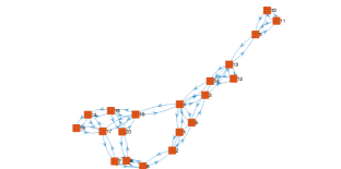
Figure 2: The social network with $20$ nodes considered in our test.

To analyze the impact of the policies designed with the proposed strategy we consider a randomly generated graph with $20$ nodes, with 7 clusters, a total link probability equal to $0.2$, and a probability of connections among nodes in different clusters equal to 0.7. The initial inclination of $20$ agents is drawn randomly from a uniform distribution in $[0,1]$, while the relative weights of social influence $[\lambda]$ are chosen here to be equal for all agents, i.e., $\lambda_{v}=\lambda$ for all $v=1,\ldots,20$. Despite this simplification, we still analyze two different cases with $\lambda=0.25$ and $\lambda=0.75$. These choices represent two opposite situations, with the former entailing that the agents change their inclination mainly based on their bias and external interventions, and the latter implying that the main drivers to one’s inclination are social influences.

Apart from the initial conditions, the other source of differentiation between agents is represented by the values of $u_{\mathrm{o}}$, for which we consider four different scenarios.

1. Firstly, we consider $u_{\mathrm{o},v}=0.7$ for all $v\in\mathcal{V}$, which implies a pre-existing positive bias within the population.

2. Then, we consider the case in which $10$ agents have $u_{\mathrm{o},v}=0.2$ and the remaining 10 have $u_{\mathrm{o},v}=0.8$. This implies that the population’s bias is skewed, with half of it represented by what can be seen as less receptive agents.

3. As a third scenario, we consider a heterogeneous population, where individuals are generally positively biased. In this case, half of the agents (i.e., $10$) are characterized by $u_{\mathrm{o},v}=0.6$ and the remaining half has an initial bias of $0.8$.

4. At last, we consider the completely opposite situation of an overall more receptive population with half of the agents having an initial bias of 0.2 and the remaining ones having $u_{\mathrm{o},v}=0.3$.

We design and apply the proposed policies over a horizon of $T=30$ steps and, to evaluate its outcome, we consider three quality indicators. As an empirical check of recursive feasibility, we evaluate (if any) the number of time instant $\tau^{\mathrm{ob}}$ in which the actual (inaccessible) inclination exceeds the interval $[0,1]$. This indicator allows us to assess the benefit of the worst-case approach adopted to cope with (unpredictable) external factors. As a second quality indicator, we consider the average number of adopters $\Gamma_{T}$ over time, i.e.,

$$\Gamma_{T}=\frac{1}{|\mathcal{V}|T}\sum_{t=0}^{T-1}\sum_{v\in V}y_{v}(T)\cdot 100,~{}~{}[\%]$$ (22)

which ultimately provides us with an indication of the effectiveness of each policy strategy at the end of the considered horizon. An actual cost-benefit analysis cannot be carried out without considering an additional indicator, i.e.,

$$\Delta u^{c}_{T}=\sum_{t=0}^{T-1}\|u^{c}(t)\|_{1},$$ (23)

which provides insight into the overall effort required to enact a given policy. In the following, we denote the conservative policy obtained by solving the worst-case problem (see Eq. (13)) as (WC), and the time-varying solution as (TV). Note that in both these cases the state is fully acessible. When estimating the state (in the absence of external disturbances), we solely test the latter policy, indicating such test with (E-TV). To design all these policies, we set $r=0.1$, $\alpha=0.99$ and $\delta=0.025$. Future work will be devoted to analyzing the impact of these tuning variables on policy behavior.

IV-A Policy impact in the noise-free case

TABLE I: Disturbance-free case: indicators for $\lambda=0.25$

	$\Gamma_{T}$ (WC)	$\Gamma_{T}$ (TV)	$\Gamma_{T}$ (E-TV)	$\Delta u^{c}_{T}$ (WC)	$\Delta u^{c}_{T}$ (TV)	$\Delta u^{c}_{T}$ (E-TV)
Case 1	94.83 %	87.24 %	88.10 %	5.29	3.70	3.54
Case 2	92.76 %	81.72 %	81.38 %	8.78	6.67	6.43
Case 3	93.62 %	85.34 %	88.10 %	5.29	3.78	3.72
Case 4	88.96 %	76.90 %	79.48 %	13.23	10.06	10.06

TABLE II: Disturbance-free case: indicators for $\lambda=0.75$

	$\Gamma_{T}$ (WC)	$\Gamma_{T}$ (TV)	$\Gamma_{T}$ (5-TV)	$\Delta u^{c}_{T}$ (WC)	$\Delta u^{c}_{T}$ (TV)	$\Delta u^{c}_{T}$ (E-TV)
Case 1	91.38 %	88.10 %	90.17 %	5.30	4.66	5.44
Case 2	89.13 %	86.03 %	89.13 %	8.64	7.99	8.75
Case 3	92.59 %	87.07 %	91.90 %	5.27	4.69	5.35
Case 4	88.79 %	87.93 %	88.97 %	13.19	12.71	13.73

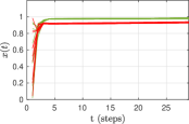
((a)) Hidden inclinations (WC)

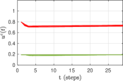
((b)) Policy actions (WC)

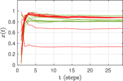
((c)) Hidden inclinations (E-TV)

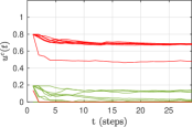
((d)) Policy actions (E-TV)

Figure 3: Disturbance-free case: states and inputs for the best-performing policies, i.e., (WC) and (E-TV) for scenario 2 and $\lambda=0.25$ over time. The green curves are associated with agents with positive bias ($u_{\mathrm{o},v}=0.8$), while the red ones are associated with agents having $u_{\mathrm{o},v}=0.2$.

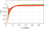
((a)) Hidden inclinations (WC)

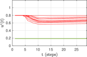
((b)) Policy actions (WC)

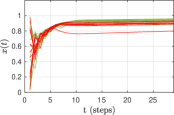
((c)) Hidden inclinations (TV)

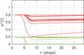
((d)) Policy actions (TV)

Figure 4: Disturbance-free case: states and inputs for the best-performing policies, i.e., (WC) and (TV) for scenario 2 and $\lambda=0.75$ over time. The green curves are associated with agents with positive bias ($u_{\mathrm{o},v}=0.8$), while the red ones are associated with agents having $u_{\mathrm{o},v}=0.2$.

Tables I-II report the value of the indicators for all the considered scenarios. Independently on the value of $[\lambda]$ (in this nonetheless constant across agents), the worst-case conservative law obtained by solving Eq. (13) is the one generally resulting in the most widespread diffusion of a positive inclination. This generally comes at the price of an increased policy cost. From this perspective, the policies with adapting weights tend to outperform the “brute-force” approximation performed in Eq. (10). This confirms the capability of the latter policy to better adapt to changes in individual inclinations (despite the approximation performed in constructing the weights) and, hence, allow policymakers to save money.

Both Tables I-II show a general tendency of costs to increase when more agents tend to be receptive to the policy, while inherently negatively biased. As one would have guessed intuitively, containing investments in such a scenario might be counterproductive. Meanwhile, comparing the results in these tables, it can be noticed that all policies tend to be closer in performance and cost for a higher $\lambda$, showcasing the impact that different degrees in social connection can have on the final policy outcome and cost-benefit trade-off. At the same time, these results do not show any specific drop in performance, validating the use of the “simple” estimate Eq. (20) to reconstruct the (hidden) state, at least in this relatively simple example.

Focusing on the “skewed” scenario (i.e., scenario 2), Figure 3 and Figure 4 show the evolution of the hidden state (a.k.a., inclinations) of all agents over time, along with the policies enacted to achieve such result. From these plots, the difference between the two conditions on $\lambda$ and, hence, the effect of social interactions is clear. A higher $\lambda$ indeed promotes agents’ inclination to evolve more cohesively, with few agents left behind at the price of a slower achievement of a widespread positive inclination. Also when looking at the policy actions, the changes required by different levels of social connections are clear. In particular, when $\lambda=0.75$, policy actions tend to be more varied (especially for negatively biased agents) indicating the need for policymakers to counteract the effect induced by social interaction and individual biases in a more dedicated way. Last but not least, the results obtained when exploiting the estimated state rather than the actual state (see the lower side of Figure 3) are still consistent with the general trend observed when the true (but practically unknown state) is available. At the same time, small oscillations appear in the transient of both the state and the input, spotlighting the fact that approximate information is employed for policy design.

IV-B Policy impact with external disturbances

TABLE III: Noisy case: indicators for $\lambda=0.25$

	$\Gamma_{T}$ (E-WC)	$\Gamma_{T}$ (E-TV)	$\Delta u^{c}_{T}$ (E-WC)	$\Delta u^{c}_{T}$ (E-TV)
Case 1	96.55 %	87.59 %	5.37	3.62
Case 2	93.79 %	80.17 %	8.83	6.51
Case 3	95.51 %	88.62 %	5.40	3.74
Case 4	91.55 %	72.41 %	13.18	9.63

TABLE IV: Noisy case: indicators for $\lambda=0.75$

	$\Gamma_{T}$ (E-WC)	$\Gamma_{T}$ (E-TV)	$\Delta u^{c}_{T}$ (E-WC)	$\Delta u^{c}_{T}$ (E-TV)
Case 1	92.24 %	91.38 %	5.58	5.38
Case 2	90.69 %	90.68 %	9.26	8.85
Case 3	93.10 %	90.52 %	5.60	5.46
Case 4	90.52 %	90.52 %	13.66	13.43

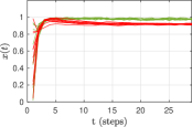
((a)) Hidden inclinations (E-WC)

((b)) Policy actions (E-WC)

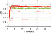
((c)) Hidden inclinations (E-TV)

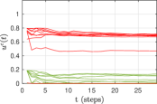
((d)) Policy actions (E-TV)

Figure 5: Noisy case: states and inputs for (E-WC) and (E-TV) for scenario 2 and $\lambda=0.25$ over time. The green curves are associated with agents with positive bias ($u_{\mathrm{o},v}=0.8$), while the red ones are associated with agents having $u_{\mathrm{o},v}=0.2$.

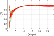
((a)) Hidden inclinations (E-WC)

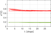
((b)) Policy actions (E-WC)

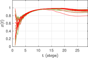
((c)) Hidden inclinations (E-TV)

((d)) Policy actions (E-TV)

Figure 6: Noisy case: states and inputs for (E-WC) and (E-TV) for scenario 2 and $\lambda=0.75$ over time. The green curves are associated with agents with positive bias ($u_{\mathrm{o},v}=0.8$), while the red ones are associated with agents having $u_{\mathrm{o},v}=0.2$.

When considering the impact of external disturbances, we evaluate the same performance criteria as before focusing only on the worst-case policy designed via the mean inclination estimate (E-WC) and the one obtained with such estimate and time-varying weights. The attained performance indicators are reported in Tables III-IV for both the conditions on $\lambda$, showing that the trends evidenced in the absence of noise are confirmed when (unpredictable) external disturbances impact individual inclinations. At the same time, at least in our example, this shows that the estimate for the mean inclinations can represent an asset in the absence of direct insight into individual beliefs (which are anyway unrealistic in practice).

Mimicking the analysis performed in the disturbance-free case, in Figure 5 and Figure 6 we show the (hidden) inclination and (controlled) input trajectories obtained for the two considered policies and the two scenarios on $\lambda$. Once again, the results we obtain are consistent with those achieved in the disturbance-free case, despite slightly deteriorated by the uncertainty on the initial condition of the receding horizon controllers and the presence of $u^{nc}$.

V Concluding Remarks

This work presented a model-based framework to analyze the impact of external interventions on the evolution of individual inclinations subject to social influences and the effects of unpredictable phenomena (i.e., changes in the weather forecast when deciding to use a shared bicycle). This formalization has allowed us to devise a set of optimal policy design strategies, aimed at minimizing quadratic approximations of an economic cost by looking at the balance between fostering adoption and containing costs. Our numerical analysis spotlighted the differences, benefits, and drawbacks of the proposed strategies, setting the ground for further research into the use of these models for effective policy design in a social setting.

Future work will be devoted to proving the theoretical guarantees on the performance of the proposed policy design schemes, along with considering the full cost without approximations and, hence, a stochastic policy design problem, and validating the approaches on real-world applications.

References

- [1] N. E. Friedkin, “A formal theory of social power,” Journal of Mathematical Sociology, vol. 12, pp. 103–126, 1986.
- [2] N. E. Friedkin and E. C. Johnsen, “Social influence and opinions,” Journal of Mathematical Sociology, vol. 15, no. 3–4, pp. 193–206, 1990.
- [3] V. Breschi, C. Ravazzi, S. Strada, F. Dabbene, and M. Tanelli, “Driving electric vehicles’ mass adoption: An architecture for the design of human-centric policies to meet climate and societal goals,” Transportation Research Part A: Policy and Practice, vol. 171, p. 103651, 2022.
- [4] ——, “Fostering the mass adoption of electric vehicles: A network-based approach,” IEEE Transactions on Control of Network Systems, vol. 9, no. 4, pp. 1666–1678, 2022.
- [5] W. S. Rossi, J. W. Polderman, and P. Frasca, “The closed loop between opinion formation and personalized recommendations,” IEEE Transactions on Control of Networked Systems, vol. 9, no. 3, pp. 1092–1103, 2022.
- [6] J. Castro, J. Lu, G. Zhang, Y. Dong, and L. Martínez, “Opinion dynamics-based group recommender systems,” IEEE Transactions on Systems, Man, and Cybernetics: Systems, vol. 48, no. 12, pp. 2394–2406, 2018.
- [7] M. Goyal, D. Chatterjee, N. Karamchandani, and D. Manjunath, “Maintaining ferment,” in Proc. of the 2019 IEEE 58th Conference on Decision and Control (CDC), 2019, pp. 5217–5222.
- [8] B. Sprenger, G. De Pasquale, R. Soloperto, J. Lygeros, and F. Dörfler, “Control strategies for recommendation systems in social networks,” arXiv preprint arXiv:2403.06152, 2024.
- [9] P. Frasca, C. Ravazzi, R. Tempo, and H. Ishii, “Gossips and prejudices: Ergodic randomized dynamics in social networks,” IFAC Proceedings Volumes, vol. 46, no. 27, pp. 212–219, 2013.
- [10] C. Ravazzi, P. Frasca, R. Tempo, and H. Ishii, “Ergodic randomized algorithms and dynamics over networks,” IEEE Transactions on Control of Network Systems, vol. 2, no. 1, pp. 78–87, 2015.
- [11] E. Polak and T. H. Yang, “Moving horizon control of linear systems with input saturation and plant uncertainty part 1. robustness,” International Journal of Control, vol. 58, no. 3, pp. 613–638, 1993.