Orbital paramagnetism without density of states enhancement
in nodal-line semimetal ZrSiS

Abstract

Unconventional orbital paramagnetism without enhancement of the density of states was recently discovered in the nodal-line semimetal ZrSiS. Here, we propose a novel interband mechanism of orbital paramagnetism associated with the negative curvature of energy dispersions, which successfully explains the observed anomalous orbital paramagnetism. This negative curvature arises from energy fluctuations along the nodal line, inherent in realistic nodal-line materials. Our new mechanism indicates that such orbital paramagnetism serves as strong evidence for the existence of nodal lines not only in ZrSiS but potentially in various other nodal-line materials as well.

Orbital magnetism is one of the fundamental properties of solids, rooted in the seminal research of Landau and Peierls on free electron and tight-binding models [1, 2]. In Dirac electron systems such as bismuth and graphene, significant orbital diamagnetism arises from the interband effect of a magnetic field [3, 4, 5, 6, 7]. This discovery has shown that orbital magnetism is highly sensitive to the band structure of crystals, leading to extensive research into their relationship that has continued to this day. Orbital magnetism is also a bulk property that probes the unique energy dispersions and wave functions of electronic states with nontrivial topology, such as those in Weyl semimetals [3, 7, 8, 4, 5, 9, 9, 10, 11, 6, 12, 13] and topological insulators [14, 15, 16, 17]. We expect orbital magnetism to also characterize nodal-line semimetals [18, 19, 20, 21, 22, 23, 24], which are usually confirmed through a combination of angle-resolved photoemission spectroscopy [25, 26, 27], quantum oscillations [28, 29, 30], and transport phenomena [23, 24, 7, 31, 32, 33, 34, 35].

Recently, unconventional paramagnetism was observed in the nodal-line semimetal ZrSiS at low temperatures when a magnetic field is applied along the $C_{4}$ rotation axis [30]. This paramagnetism is not explained by the Pauli paramagnetism estimated from the observed low density of states (DOS). Additionally, when the magnetic field is applied perpendicular to the $C_{4}$ axis, ZrSiS exhibits diamagnetism, showing strong anisotropy. These results strongly suggest that the unconventional behaviors of ZrSiS originate from the orbital effect rather than the spin effect. A similar paramagnetism has been observed in another nodal-line semimetal SrAs₃ [36]. Furthermore, as the temperature increases, the paramagnetism along the $C_{4}$ axis of ZrSiS decreases and eventually changes to diamagnetism at around 120K, which is also an unexpected behavior. Despite several efforts to understand these anomalous behaviors, their microscopic origins, probably due to the nodal line [30, 37], remain elusive.

At present, a few origins of orbital paramagnetism are known, including the Van Hove singularity [38, 39], flatband [40, 41], and other mechanisms [37, 42]. In most of these cases, however, orbital paramagnetism is accompanied by a strong enhancement of a DOS, and thus it is concealed by the large Pauli paramagnetism. In this Letter, we propose a new mechanism to explain the orbital paramagnetism without an enhanced DOS. We first present a quantitative analysis of the orbital magnetic susceptibility in ZrSiS using the density functional theory (DFT) calculations and the effective models based on them, successfully illustrating the observed paramagnetism, temperature dependence, and anisotropy. To further understand the origin of this orbital paramagnetism, we derive a simple effective model. The analysis of it shows that the observed orbital paramagnetism without DOS enhancement is attributed to the interband effect between two energy dispersions with negative curvature. This negative curvature originates from the energy fluctuation along the nodal line, which is inherent in realistic nodal-line materials. This novel mechanism indicates that such orbital paramagnetism serves as strong evidence for the nodal lines not only in ZrSiS but potentially in various other nodal-line materials as well.

DFT calculations and models.—

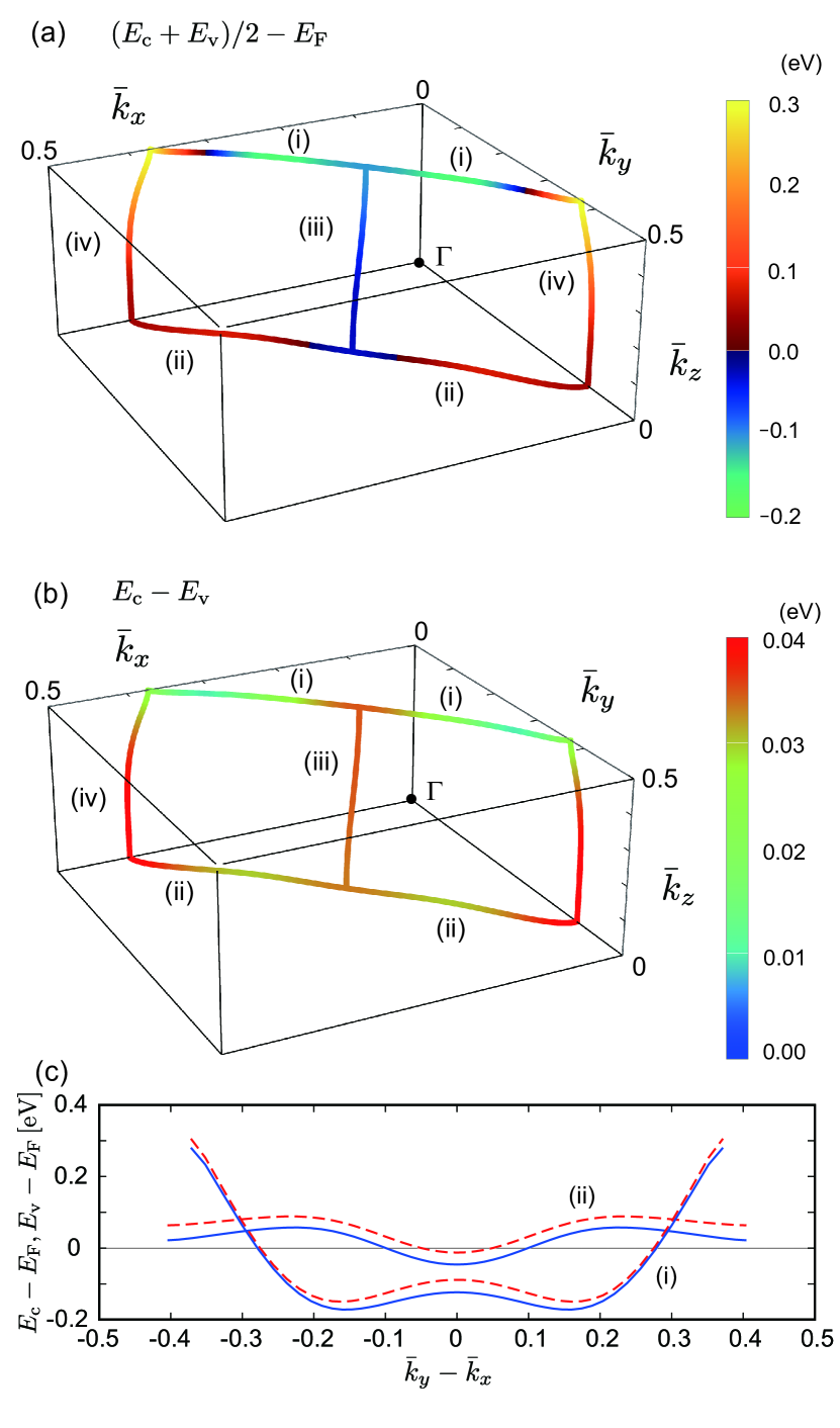
Figure 1: Positions of the nodal points in the Brillouin zone. The dimensionless wave numbers $\bar{k}_{x}=k_{x}a/(2\pi)$, $\bar{k}_{y}=k_{y}a/(2\pi)$, and $\bar{k}_{z}=k_{z}c/(2\pi)$ are shown. (a) Color indicates the energy of the middle of the gap $(E_{c}({\bm{k}})+E_{v}({\bm{k}}))/2-E_{F}$ with $E_{c}({\bm{k}})$ and $E_{v}({\bm{k}})$ being the energy of the bottom (top) of the conduction (valence) band at $\bm{k}$, and $E_{\rm F}$ is the Fermi energy. (b) Color indicates the magnitude of the gap due to the SOI, $E_{c}({\bm{k}})-E_{v}({\bm{k}})$. (c) Energy dispersions near $E_{\rm F}$ along the nodal lines (i) and (ii). The valence (conduction) band is shown in solid (dashed) line.

ZrSiS has a $P4/mnn$ structure [43, 44] and has a set of nodal lines [45, 30, 46, 47]. To capture the characteristics of these nodal lines in detail, we perform DFT calculations using Quantum-ESPRESSO and Wannier90 packages [48, 49, 50, 51, 52, 53] with the lattice parameters of $a=3.55$ Å and $c=8.07$ Å [54]. The details of this calculation are shown in Supplemental Material (SM) [55]. Figure 1 shows the positions of the nodal points in the Brillouin zone, at which the bottom of the conduction band ($E_{c}({\bm{k}})$) and the top of the valence band ($E_{v}(\bm{k})$) are close to each other. The colors in Fig. 1(a) indicate the energy of the middle of the gap relative to the Fermi energy $E_{F}$, i.e., $(E_{c}(\bm{k})+E_{v}(\bm{k}))/2-E_{F}$, and those in Fig. 1 (b) indicate the magnitude of the gap $E_{c}(\bm{k})-E_{v}(\bm{k})$ due to the spin-orbit interaction (SOI). Four nodal lines (i) – (iv) are indicated, which are in the planes of $k_{z}=\pi/c$, $k_{z}=0$, $|k_{x}|=|k_{y}|$, and $k_{x}=0$ or $k_{y}=0$, respectively. Note that the nodal line protected by the nonsymmorphic symmetry [45] is omitted because it is approximately 1eV away from $E_{F}$. From Fig. 1(a), we can see that the nodal lines (i) and (ii) form closed lines in the Brillouin zone on the $k_{z}c=\pi$ and $k_{z}c=0$ planes, respectively, both of which cross $E_{F}$. As shown in Fig. 1 (c), the energy deviations around $E_{F}$ are about $\pm 0.25$ eV for (i) and $\pm 0.05$ eV for (ii), which play important roles in the later calculations. The nodal lines (iii) and (iv) form one-dimensional lines along the $k_{z}$ direction. While the nodal line (iii) is located close to $E_{F}$, (iv) is away from $E_{F}$, so that we neglect the nodal line (iv) in the following.

Considering these characteristics of ZrSiS, we introduce an effective model for the nodal lines (i) and (ii) as

$${\mathcal{H}}^{\text{(X)}}=\biggl{[}\frac{\hbar^{2}}{2m^{*}}(k_{x}^{2}+k_{y}^{2})-\Delta\biggr{]}\sigma_{z}+\hbar v_{z}k_{z}\sigma_{x}+\eta^{\text{(X)}}(k_{x}^{2}-k_{y}^{2})\sigma_{0},$$ (1)

where X=i or ii is the index for the nodal lines and $\sigma_{0}$, $\sigma_{x}$, and $\sigma_{z}$ are the identity and Pauli matrices. The first term represents the two parabolic bands with masses of different signs. As shown in Fig. 2, the overlap of the bands is $2\Delta$. The second term in Eq. (1) hybridizes the two bands where $v_{z}$ represents the velocity in the $z$ direction. The ${\bm{k}}$ points on the nodal line satisfies $\frac{\hbar^{2}}{2m^{*}}(k_{x}^{2}+k_{y}^{2})-\Delta=0$ and $k_{z}=0$, indicating that the nodal line forms a circle in the $k_{x}$-$k_{y}$ planes at $E_{F}=0$. The last term gives the fluctuation of energy along the nodal line, and the energy deviation is $\pm 2\eta^{\text{(X)}}k_{\rm R}^{2}$ with $k_{\rm R}=\sqrt{2m^{*}\Delta}/\hbar$ being the radius of the nodal line. The similar energy fluctuation has been discussed in Refs. [37, 56, 57, 58, 31]. In the following, we omit the superscript of $\eta$ when distinction is not necessary.

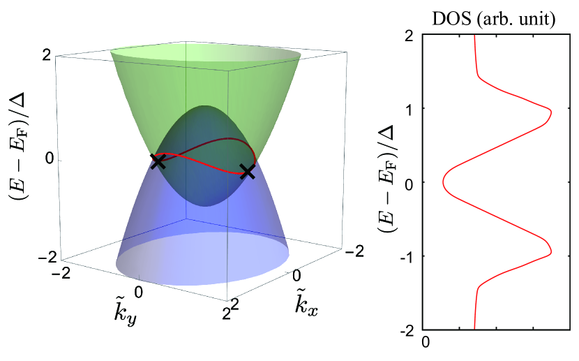
Figure 2: Energy dispersions and DOS for model (1) at $k_{z}=0$ with $\tilde{\eta}=\eta k_{\rm R}^{2}/\Delta=0.2$. The red line indicates the nodal line. $\tilde{k}_{x}=k_{x}/k_{\rm R}$ and $\tilde{k}_{y}=k_{y}/k_{\rm R}$ are dimensionless wave numbers. The symbol $\bm{\times}$ indicates the nodal point at which the tangent of the nodal line is parallel to $\tilde{k}_{x}$.

Note that the effective model of Eq. (1) does not have the gap. As discussed later, the effect of gap is negligible when we compare the results with the experiment.

The nodal line (iii) is approximately regarded as 2D Dirac electrons, governed by

$$\mathcal{H}^{\text{(iii)}}=\hbar v_{\rm Dirac}(k_{x}\sigma_{x}+k_{y}\sigma_{y})+\Delta_{\rm SOI}\sigma_{z}+\varepsilon_{0}(k_{z}),$$ (2)

where $\varepsilon_{0}(k_{z})$ is the energy shift and $\Delta_{\rm SOI}$ represents the gap originating from SOI. We discuss the orbital magnetic susceptibility using models (1) and (2) in the following.

Orbital magnetic susceptibility.— The orbital magnetic susceptibility in a magnetic field in the $z$ direction ($\chi_{z}$) is generally given by [59]

$$\chi_{z}=\frac{e^{2}}{\hbar^{2}}k_{B}T\sum_{n{\bm{k}}}{\rm Tr}\,\gamma_{x}{\mathcal{G}}\gamma_{y}{\mathcal{G}}\gamma_{x}{\mathcal{G}}\gamma_{y}\mathcal{G},$$ (3)

where ${\mathcal{G}}=\mathcal{G}({\bm{k}},i\varepsilon_{n})=[i\varepsilon_{n}-\mathcal{H}^{\text{(X)}}+\mu]^{-1}$ is the thermal Green’s function, $\varepsilon_{n}=(2n+1)\pi k_{\rm B}T$ ($n\in\mathbb{Z})$ is the Matsubara frequency, and $\gamma_{i}$ is the velocity operator of in the $i$ ($i=x,y,z$) direction defined by $\gamma_{i}=\frac{\partial{\mathcal{H}}^{\text{(X)}}}{\partial k_{i}}$. This formula has included the spin degeneracy. The orbital magnetic susceptibility in other directions is obtained by a cyclic replacement of $x$, $y$, and $z$. We numerically evaluate Eq. (3) for the model (1), employing the quasi-Monte Carlo method [60, 61, 62, 63, 64] for ${\bm{k}}$ summation, and the sparse-ir method [65, 66, 67] for Matsubara summation. The cutoff for ${\bm{k}}$ integral is set to $\Lambda_{\rm R}=1000k_{\rm R}$ in the radial direction and $\Lambda_{z}=(l_{z})^{-1}$ in the $z$ direction with $l_{z}=\hbar v_{z}/\Delta$. The results for $\chi_{z}$ and $\chi_{x}$ are shown in Fig. 3 (a) and (b), respectively, for several values of $\tilde{\eta}=\eta k_{\rm R}^{2}/\Delta$. For the case without the energy fluctuation ($\tilde{\eta}=0$), $\chi_{z}$ is diamagnetic for every $\mu$ while $\chi_{x}$ has a sharp peak at $\mu=0$ originating from the interband effect of the 2D Dirac electrons [6]. It is confirmed that our calculation reproduces the previous results [24] in the limit of $\Lambda_{\rm R}\to\infty$ and $\Lambda_{z}\to\infty$ [see SM[55] for detail].

Finite $\eta$ gives a drastic effect on $\chi_{z}$: $\chi_{z}$ has a broad peak around $\mu=0$, whose width is approximately $2\eta k_{\rm R}^{2}$. Furthermore, for $\tilde{\eta}>0.1$, the value at the peak is positive, meaning orbital paramagnetism. The inset of Fig. 3 (a) shows the Landau-Peierls (LP) contribution [1, 2, 39, 68], or the intraband contribution, which is negative for all the value of $\mu$. Therefore, we conclude that the obtained orbital paramagnetism near $\mu=0$ is due to an interband effect. As we noted before, the orbital paramagnetism is usually accompanied by a large DOS, while the present result suggests an interband orbital paramagnetism without the enhancement of the DOS. Note that the DOS near $\mu=0$ is small as shown in Fig. 2. The mechanism is discussed in detail later.

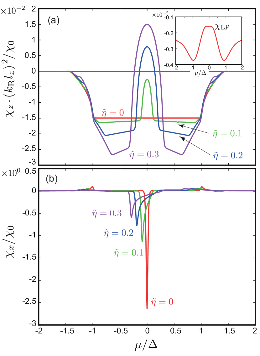
Figure 3: (a) Orbital magnetic susceptibility $\chi_{z}$ as a function of chemical potential when $k_{B}T=0.01\Delta$ for several values of $\tilde{\eta}=\eta k_{\rm R}^{2}/\Delta$. (b) Orbital magnetic susceptibility $\chi_{x}$ when $k_{B}T=0.05\Delta$. They are normalized by $\chi_{0}\equiv\frac{e^{2}}{\hbar^{2}}Vl_{z}\Delta$ with $V$ being the volume and $l_{z}=\hbar v_{z}/\Delta$. Inset: LP contribution for $\tilde{\eta}=0.3$ and $k_{B}T=0.1\Delta$.

As shown in Fig. 3 (b), $\chi_{x}$ is not an even function of the chemical potential for finite $\eta$. We find the relations $\chi_{x}(\mu,\eta)=\chi_{x}(-\mu,-\eta)$ and $\chi_{x}(\mu,\eta)=\chi_{y}(-\mu,\eta)$ from the analytical expressions, shown in SM [55]. This behavior is understood as follows. At each point on the nodal line, a Dirac dispersion $\propto\pm\sqrt{q_{x}^{2}+q_{y}^{2}}$ is formed, where $q_{x}$-$q_{y}$ plane is perpendicular to the tangent of the nodal line at the point. Therefore, when the magnetic field is parallel to the tangent of the nodal line, the delta function–like orbital diamagnetism ($\propto-\delta(\mu-\varepsilon_{0}))$ [59, 6] is negatively maximized with $\varepsilon_{0}$ being the energy of the Dirac point. As we can see from the symbol $\times$ in Fig. 2, when $\eta$ is positive, the energy of the nodal point at which the tangent of the nodal line is parallel to $\tilde{k}_{x}$ is negative, i.e., $\varepsilon_{0}<0$. Thus, $\chi_{x}$ takes the negatively maximal value at $\mu=\varepsilon_{0}<0$. The magnitude of $\chi_{x}$ becomes smaller as $\eta$ increases, since the region of the nodal line parallel to $\tilde{k}_{x}$ becomes smaller.

Comparison with experiments.— We evaluate the orbital magnetic susceptibility for ZrSiS using the parameters obtained by the DFT calculations. For $\chi_{z}$, we consider $\chi_{z}^{\rm tot}=\chi_{z}^{\text{(i)}}+\chi_{z}^{\text{(ii)}}+\chi_{z}^{\text{(iii)}}+\chi_{\rm Pauli}$, where $\chi_{z}^{\text{(X)}}$ represents the contribution from the nodal line X (X=i, ii, iii), and the Pauli paramagnetism $\chi_{\rm Pauli}=0.125\times 10^{-4}$ emu/mol [30] is included. We evaluate $\chi_{z}^{\text{(i)}}$ and $\chi_{z}^{\text{(ii)}}$ from Eq. (1). $\chi_{z}^{\text{(iii)}}$ is obtained from the model (2) by the $k_{z}$ average of the known result for the 2D Dirac electron system [39]

$$\chi_{2D}(k_{z})=\frac{e^{2}v_{\rm Dirac}^{2}}{6\pi}\frac{f(\Delta_{\rm SOI},-\varepsilon_{0}(k_{z}))-f(-\Delta_{\rm SOI},-\varepsilon_{0}(k_{z}))}{\Delta_{\rm SOI}}$$ (4)

as $\chi_{z}^{\text{(iii)}}=\frac{V}{2\pi}\int dk_{z}\chi_{2D}(k_{z})$ where $f(\varepsilon,\mu)$ is the Fermi distribution function.

From the DFT calculations, we obtain $\tilde{\eta}^{\text{(i)}}=0.31$ for (i), $\tilde{\eta}^{\text{(ii)}}=0.06$ for (ii), and $\Delta_{\text{SOI}}=15$ meV and $\varepsilon_{0}(k_{z})=(-0.025-0.07|k_{z}|c/\pi)$ eV for (iii), respectively. The other parameters are adjusted to fit the experimental data [30], which are $\Delta=0.8$ eV, $m^{*}/m_{0}=0.12$, $v_{z}/c_{0}=4\times 10^{-4}$, and $v_{\rm Dirac}/c_{0}=9\times 10^{-4}$ with $m_{0}$ and $c_{0}$ being the bare electron mass and the speed of light in vacuum, respectively. Figure 4 shows the result of $\chi_{z}^{\text{tot}}$ and $\chi_{x}^{\text{tot}}$, which are in good agreement with the experiment.

Let us here discuss each contribution in $\chi_{z}^{\text{tot}}$. Since we have $\tilde{\eta}^{\text{(i)}}=0.31$ and $\tilde{\eta}^{\text{(ii)}}=0.06$, near $T=0$, $\chi_{z}^{\text{(i)}}$ is positive, while $\chi_{z}^{\text{(ii)}}$ is small and negative as shown in Fig. 3. Their sum is $\chi_{z}^{\text{(i)}}+\chi_{z}^{\text{(ii)}}=0.26\times 10^{-4}$ emu/mol, which is the main contribution for the orbital paramagnetism near $T=0$. In the temperature range of $T<300$ K, $\chi_{z}^{\text{(i)}}+\chi_{z}^{\text{(ii)}}$ is almost constant. The temperature dependence of $\chi_{z}^{\text{tot}}$ is attributed to $\chi_{z}^{\text{(iii)}}$. At low temperatures, $\chi_{z}^{\text{(iii)}}$ is negative due to the Dirac electrons in $k_{x}$-$k_{y}$ plane but small because the chemical potential is slightly outside the gap [see Fig. 1(a) and (b)]. As the temperature increases, the diamagnetism from $\chi_{z}^{\text{(iii)}}$ grows because of the smearing as expressed by Eq. (4). This leads to negative $\chi_{z}^{\text{tot}}$ when $T>120$ K.

Note that the effect of gap is not included in the model (1). However, the gap is small ($\lesssim 0.03$ eV) compared with $\Delta(=0.8$ eV), so that the effect of the gap on $\chi_{z}$ in Fig. 3 is restricted to the small range $|\mu|/\Delta\lesssim 0.04$, which will not affect our results.

Next, we consider $\chi_{x}^{\text{tot}}=\chi_{x}^{\text{(i)}}+\chi_{x}^{\text{(ii)}}+\chi_{\rm Pauli}$, where we have assumed $\chi_{x}^{\text{(iii)}}=0$ since the magnetic field is perpendicular to the nodal line. We can see that the negative value of $\chi_{x}^{\text{tot}}$ in Fig. 4 originates from $\chi_{x}$ in Fig. 3 (b).

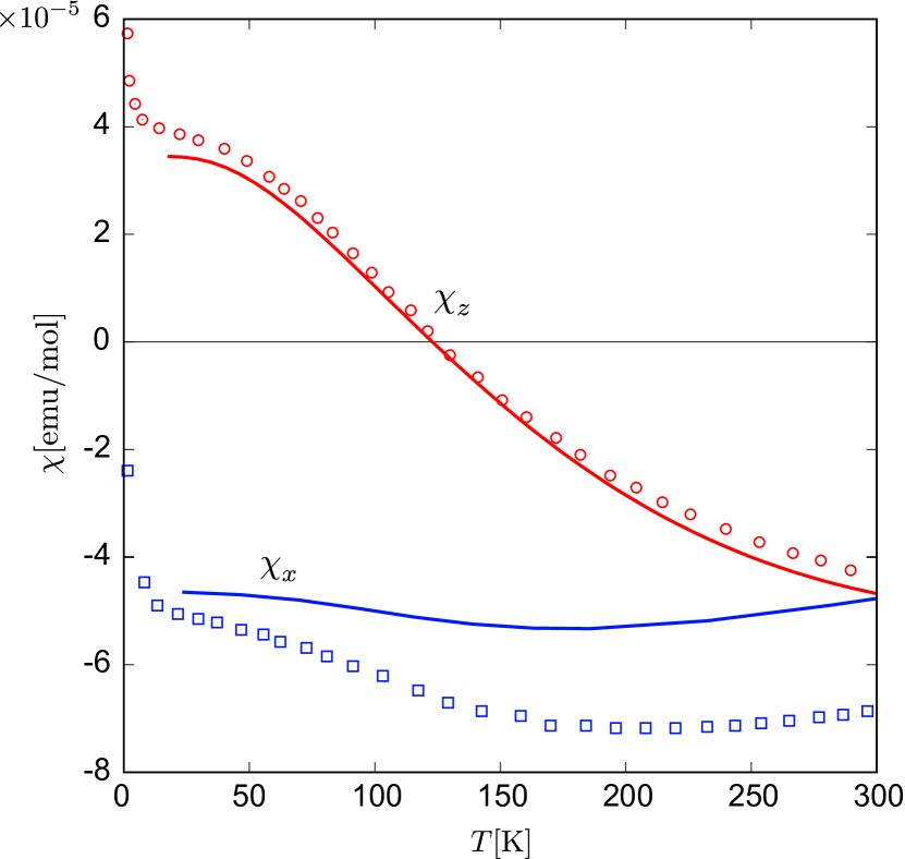
Figure 4: Temperature dependence of $\chi_{z}^{\rm tot}$ and $\chi_{x}^{\text{\rm tot}}$. Experimental data for $\chi_{z}^{\rm exp}(\bigcirc)$ and $\chi_{x}^{\rm exp}(\square)$ [30] are also shown.

Discussions.— To understand the mechanism of the interband orbital paramagnetism, which is essential for $\chi_{z}$ in ZrSiS, we introduce a simple two-band model,

$$H=\alpha\frac{k_{x}^{2}-k_{y}^{2}}{2}\sigma_{0}+\alpha\frac{k_{x}^{2}+k_{y}^{2}}{2}\sigma_{z}+\Delta\sigma_{x}.$$ (5)

This model is obtained from the small $(k_{x},k_{y})$ expansion of Eq. (1) at $(k_{x},k_{y},k_{z})=(\pm k_{\rm R},0,0)$. As shown in the inset of Fig. 5, the upper and lower bands both have saddle points. Figure 5 shows the orbital magnetic susceptibility in the $z$ direction, $\chi_{\rm orb}$, calculated by Eq. (3). The LP (intraband) contribution $\chi_{\rm LP}$ [1, 2, 39, 68] and the interband contribution ($\chi_{\rm inter}=\chi_{\rm orb}-\chi_{\rm LP}$) are also shown in Fig. 5. Our results show that this model exhibits the orbital paramagnetism near $\mu/\Delta\sim 0$ where the ground state is insulator, which is not explained by the intraband effect. The dependence on the chemical potential is similar to that observed in Fig. 3(a), indicating that the orbital paramagnetism in Fig. 3(a) is originated from the interband effect between the two saddle points. This mechanism is in sharp contrast to that of the orbital paramagnetism due to the Van Hove singularity in the single-band 2D case [38, 39] and the flat band system [40, 41], accompanied by the divergence of the DOS. Therefore, the present result of the interband orbital paramagnetism demonstrates the new mechanism that has not been known before.

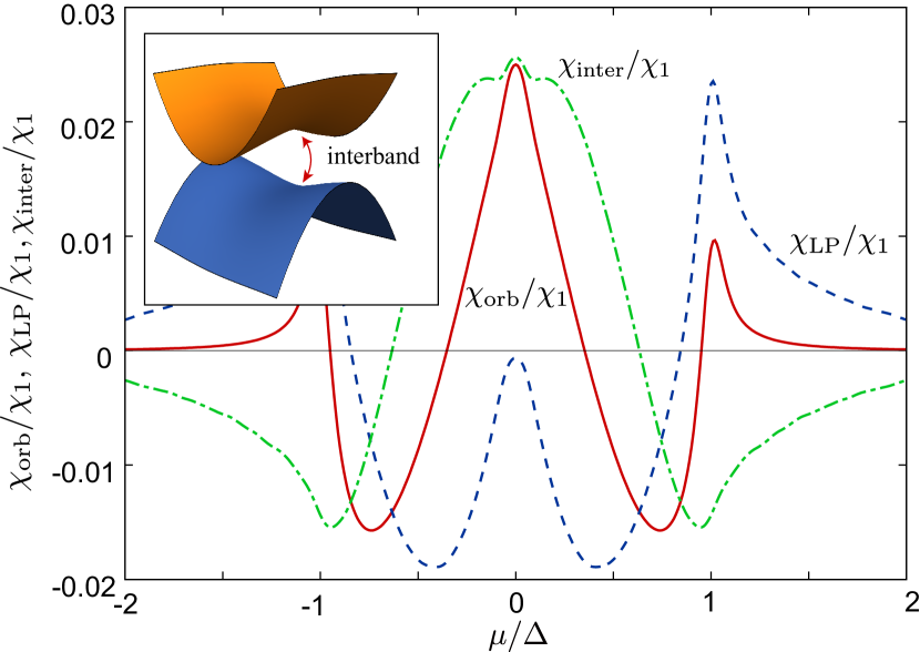
Figure 5: Total orbital magnetic susceptibility $\chi_{\rm orb}$, LP contribution $\chi_{\rm LP}$, and the interband contribution $\chi_{\rm inter}\equiv\chi_{\rm orb}-\chi_{\rm LP}$ of the saddle point model Eq. (5) in units of $\chi_{1}=e^{2}/\hbar^{2}$ with $k_{\rm B}T=1/40$ with cutoff $k_{c}=4$, where we have used the unit of $\alpha=\Delta=1$. Inset: Energy dispersions for Eq. (5).

Summary.— We have studied the orbital magnetism in ZrSiS on the basis of the DFT calculations and the effective model. Our results elucidate three anomalies of the orbital magnetism observed, the large orbital paramagnetism without DOS enhancement, temperature dependence, and paramagnetic-to-diamagnetic anisotropy. We have found that the orbital paramagnetism in the $C_{4}$ axial direction ($k_{z}$ direction) at low temperatures is attributed to the interband effect due to the energy fluctuation along the nodal line. This mechanism is new in that it is not accompanied by the diverging enhancement of the DOS, which suppresses Pauli paramagnetism and leads to observable large orbital paramangetism. This interband effect is understood in terms of the simple two-band effective model with negative curvature originating from the energy fluctuation, which is ubiquitous in realistic nodal-line materials. Therefore, these materials are promising platform where we can observe orbital paramagnetism. Orbital paramagnetism is one of the experimentally observable prominent features of nodal-line semimetals.