VoxNeuS: Enhancing Voxel-Based Neural Surface Reconstruction via Gradient Interpolation

Abstract.

Neural Surface Reconstruction learns a Signed Distance Field (SDF) to reconstruct the 3D model from multi-view images. Previous works adopt voxel-based explicit representation to improve efficiency. However, they ignored the gradient instability of interpolation in the voxel grid, leading to degradation on convergence and smoothness. Besides, previous works entangled the optimization of geometry and radiance, which leads to the deformation of geometry to explain radiance, causing artifacts when reconstructing textured planes. In this work, we reveal that the instability of gradient comes from its discontinuity during trilinear interpolation, and propose to use the interpolated gradient instead of the original analytical gradient to eliminate the discontinuity. Based on gradient interpolation, we propose VoxNeuS, a lightweight surface reconstruction method for computational and memory efficient neural surface reconstruction. Thanks to the explicit representation, the gradient of regularization terms, i.e. Eikonal and curvature loss, are directly solved, avoiding computation and memory-access overhead. Further, VoxNeuS adopts a geometry-radiance disentangled architecture to handle the geometry deformation from radiance optimization. The experimental results show that VoxNeuS achieves better reconstruction quality than previous works. The entire training process takes 15 minutes and less than 3 GB of memory on a single 2080ti GPU.

1. Introduction

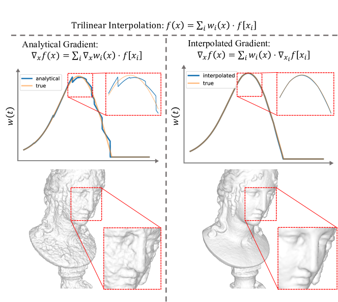
Figure 1. Previous grid-based methods adopt trilinear interpolation to retrieve SDF values and analytically solve SDF gradient. However, the gradient discontinuity leads to glitches in volume rendering weights, thus degrading the reconstruction quality. Our proposed interpolated gradient eliminates the discontinuity and smooths the reconstructed surface without additional computation overhead.

3D surface reconstruction aims to recover dense geometric scene structures from multiple images observed at different viewpoints (Hartley and Zisserman, 2003). Recently, the success of Neural Radiance Field (NeRF) (Mildenhall et al., 2021) on the novel view synthesis task proves the potential of differentiable volume rendering on fitting a density field. NeuS (Wang et al., 2021), as a representative work, uses a neural network to encode the SDF. However, the implicit representation of SDF leads to a long training time, i.e. about 8 hours for a static object.

As proved in NeRF, explicit volumetric representation achieves higher efficiency and quality than implicit representation (Müller et al., 2022; Sun et al., 2022; Fridovich-Keil et al., 2022). However, in surface reconstruction tasks, straightforward implementations result in poor geometry and undesirable noise due to the high-frequency nature of explicit volumetric representations and the multi-solution nature of volume rendering. Additional regularization is added for a reasonable surface. Voxurf (Wu et al., 2022), which directly stores SDF values in a dense grid (Sun et al., 2022), designs a dual color network to implicitly regularize the geometry, and uses total variation loss for surface smoothness. Instant NSR(Zhao et al., 2022) and NeuS2 (Wang et al., 2023a), which take iNGP’s multi-resolution hash grid (Müller et al., 2022) as the backbone, utilize multi-resolution architecture for progressive training.

These works all use grids to replace neural networks, but ignore the impact of gradients on NeuS algorithm. In volumetric representation, the SDF value or latent feature is from the trilinear interpolation of neighbouring vertices. However, the trilinear interpolation is zero order continuous only, which means that its gradient is not continuous at the grid boundary. This problem hinders convergence and the smoothness of surface, as shown in Fig. 1.

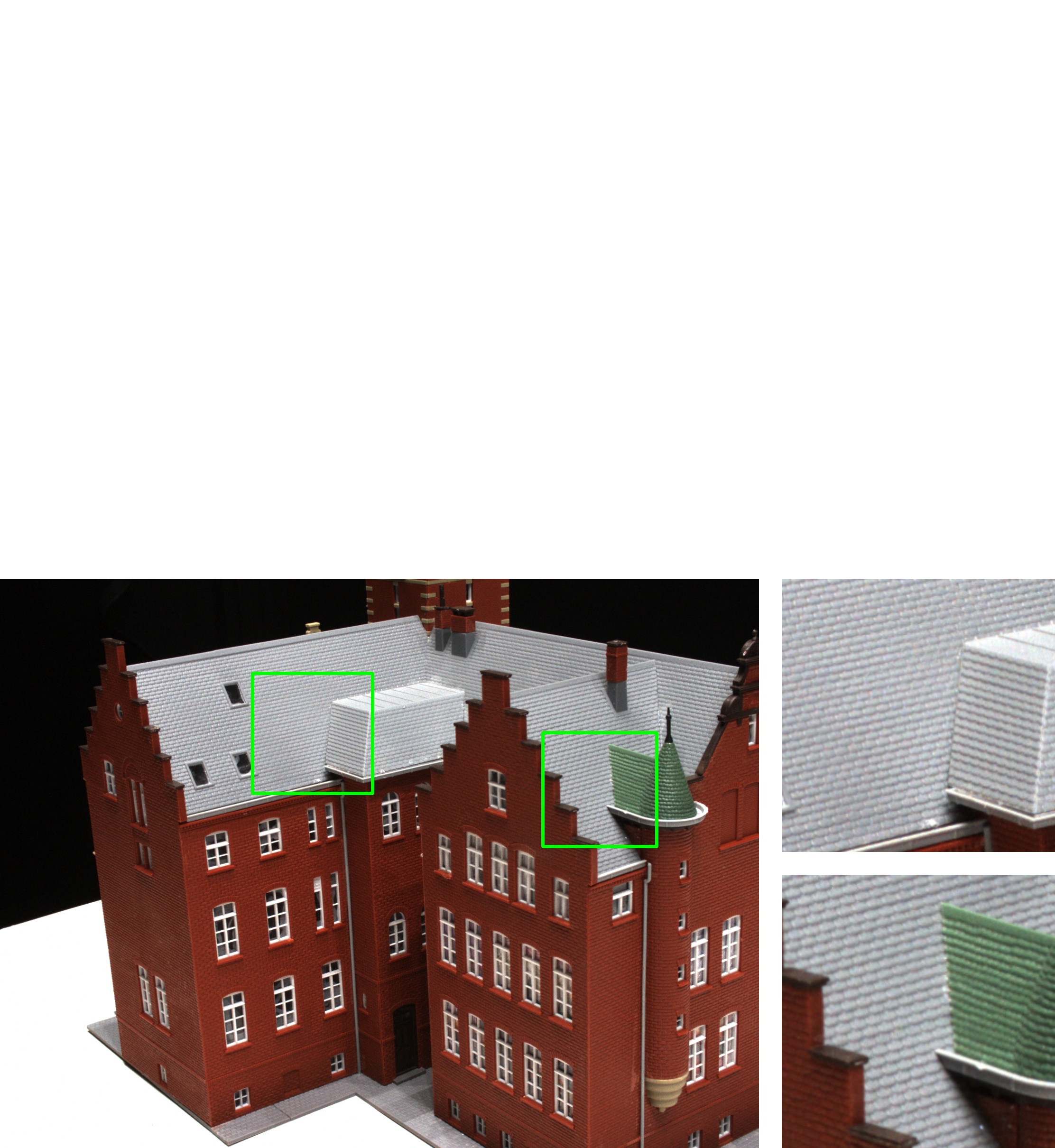
(a) Reference

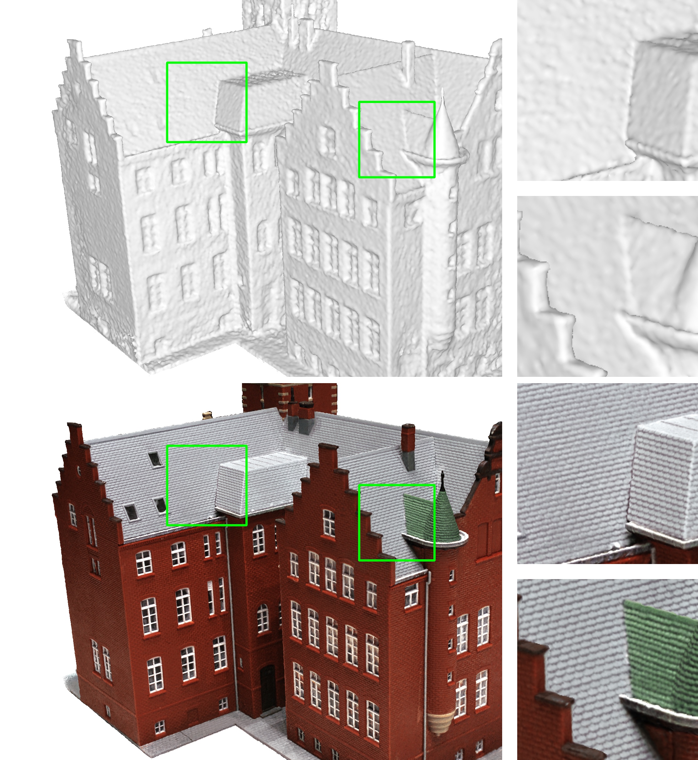
(b) Ours (15 mins; 3GB)

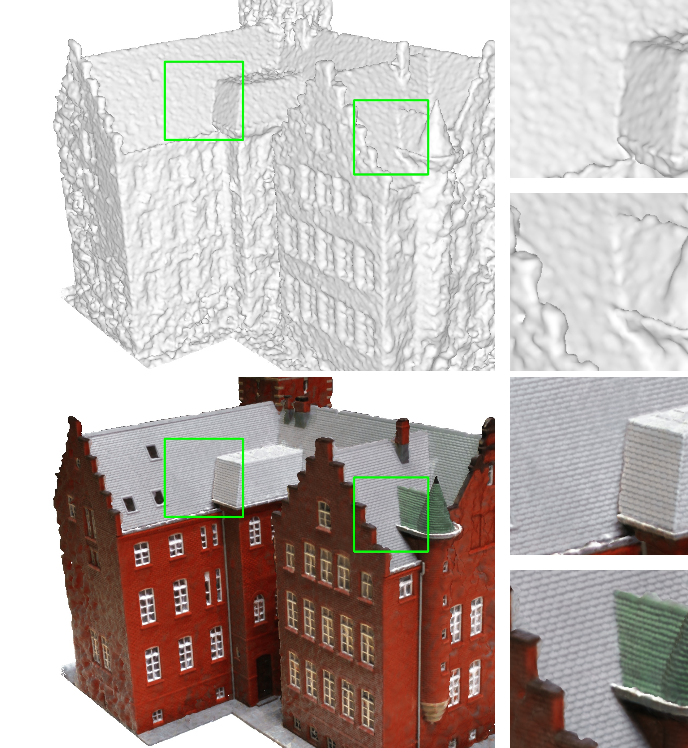
(c) w/o Interp. Grad.

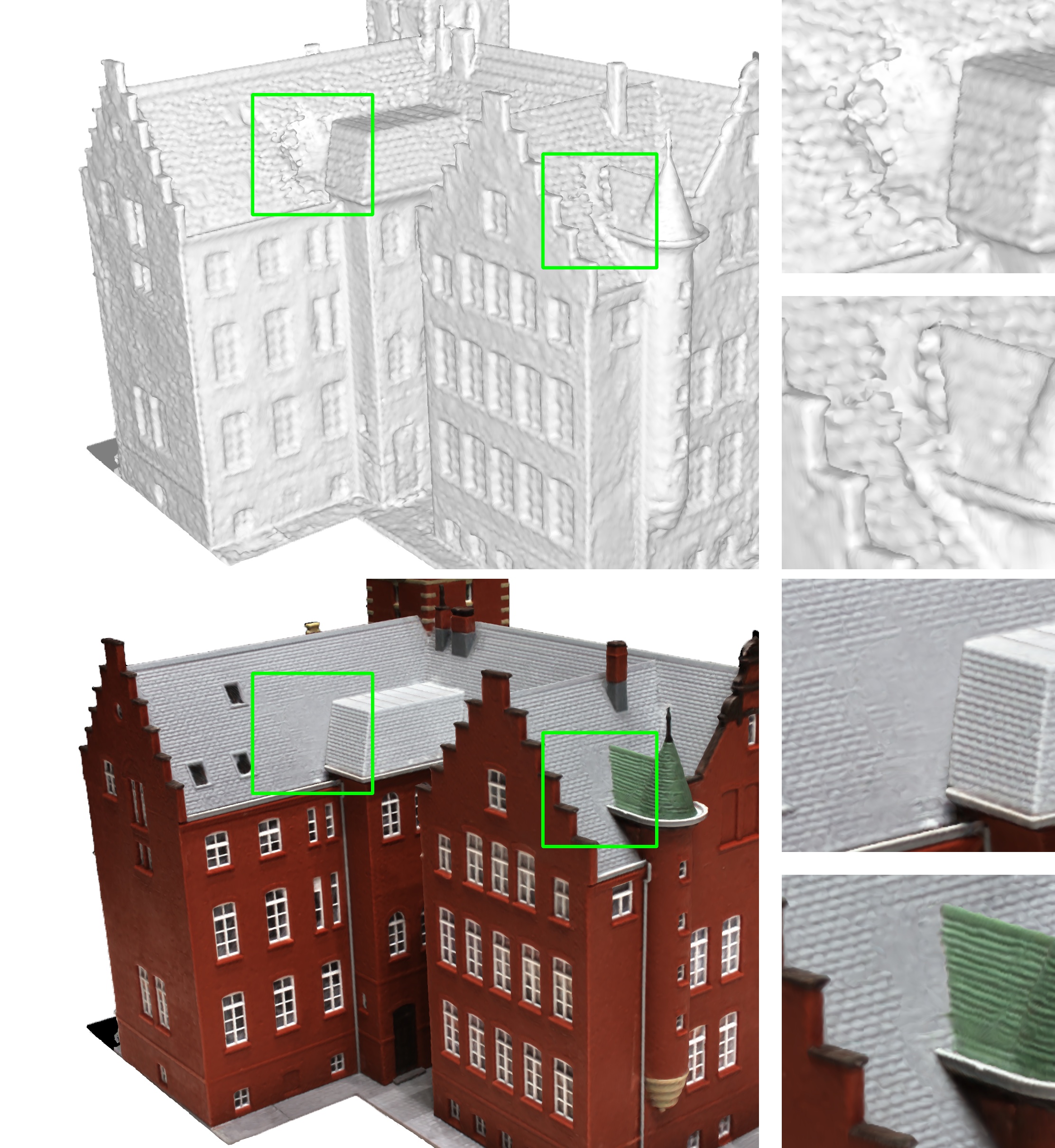
(d) Voxurf (50 mins; 14 GB)

Figure 2. Reconstruction results from different methods. The running time and GPU memory consumption are tested on a single RTX 3090 for fair comparison, as 2080ti can’t meet the memory requirement of Voxurf(Wu et al., 2022). (b) Our proposed VoxNeuS replaces analytical gradient with interpolated gradient to handle the gradient discontinuity in trilinear interpolation. Combined with a simple network structure, our method achieves efficient and high-quality reconstruction. (c) When the interpolation gradient is removed and other structures remain unchanged, the reconstruction quality drops drastically. (d) Voxurf adopts dual color network and other tricks to ease the optimization of the SDF grid, which leads to some artifacts on the surface.

When SDF is encoded by a hash grid or other hybrid representation, we need to use numerical gradients (Li et al., 2023) to eliminate gradient discontinuity, bringing the multiplied amount of the computation and memory. In contrast, when the SDF is explicitly stored in the vertices of a dense grid (Wu et al., 2022), we can directly interpolate the gradients of the vertices to ensure gradient continuity.

Based on the above analysis, we propose VoxNeuS, an efficient and lightweight surface reconstruction method that directly optimizes the SDF dense grid. In VoxNeuS, the analytical gradient is replaced with interpolated gradient to ensure continuity without additional computational overhead. With gradient interpolation, the gradient of vertices is first estimated with central finite differences. Then the target gradient is interpolated with these estimated vertex gradients to ensure zero order continuity of gradient. In addition, more designs to improve reconstruction efficiency and quality include: 1) We adopt a geometry-radiance disentangled network architecture to eliminate the impact of surface texture on geometry when fitting radiance; 2) We directly apply the gradient of the SDF regularization, i.e. Eikonal loss (Gropp et al., 2020) and curvature loss (Li et al., 2023), on vertices to avoid the overhead of forward and backward pass; 3) We leverage a progressive super-resolution of SDF grid to balance the coarse shape and fine details; 4) Critical operators like interpolation and vertices regularization are implemented in CUDA to accelerate computation and save memory, and the sparsity of gradients is considered to improve efficiency further.

The experiments are conducted on the DTU (Jensen et al., 2014) and BlendedMVS (Yao et al., 2020) datasets for quantitative and qualitative evaluations. The results demonstrate that VoxNeuS achieves a lower Chamfer Distance on the DTU benchmark than competitive volumetric-based methods, i.e. Voxurf and NeuS2. Our contributions are as following:

• We reveal that the key reason that hinders the convergence and smoothness of the NeuS in volumetric representation is the gradient discontinuity caused by trilinear interpolation.

• Our method replaces the analytical gradient of SDF with an interpolated gradient to handle the gradient discontinuity without any computational overhead.

• Our method converges well without an auxiliary foreground mask and achieves better quantitative results than competitive methods while the computational and memory efficiency improves. The training finishes in 15 minutes on a single 2080ti GPU with less than 3GB of memory cost.

2. Related Work

Neural Surface Reconstruction. Recently popular neural surface reconstruction methods use Signed Distance Function (SDF) (Green, 2007) to represent the surface. Early surface rendering methods like DVR (Niemeyer et al., 2020) and IDR (Yariv et al., 2020) seek the ray intersection point with the surface and optimize its color and coordinate. Inspired by the volume rendering, recent works densely sample points along the ray and blend their colors as ray color. NeuS (Wang et al., 2021) and VolSDF (Yariv et al., 2021) formulate equivalent density/opacity in volume rendering with SDF values. The following works (Darmon et al., 2022; Wang et al., 2022; Zhuang et al., 2023; Zhang et al., 2023; Tian et al., 2023; Ye et al., 2023) make efforts to improve the quality and efficiency. Notably, a representative method NeuS introduces the derivative of the SDF value to the coordinate as the normal in the forward pass. This mechanism benefits the convergence when the SDF is represented by an MLP. However, in the context of grid-based explicit representation where trilinear interpolation is adopted for SDF value prediction, the inaccurate estimation of gradient and the discontinuity at junction surfaces hinder the reconstruction quality drastically. Another line of work adopts recently popular 3DGS (Kerbl et al., 2023) for point-based rendering and surface reconstruction (Guédon and Lepetit, 2023; Huang et al., 2024). However, their efficiency and precision are still unsatisfactory compared to SDF-based rendering.

Volumetric Representation for Surface Reconstruction. The Signed Distance Function (SDF) was originally represented with a dense grid when proposed (Green, 2007), and neural rendering methods replace it with an MLP for easier optimization, but it leads to low efficiency during reconstruction and rendering. Therefore, volumetric-based hybrid representation is adopted for better efficiency and model capacity. Vox-surf (Li et al., 2022) uses pruned feature grid to encode SDF and color and decodes them with a shallow MLP. NeuDA (Cai et al., 2023) maintains the hierarchical anchor grids where each vertex stores a 3D position instead of the direct feature. An MLP is still required to map the deformed coordinates to geometry. The multi-resolution hash grid, proposed by iNGP (Müller et al., 2022), is applied to MonoSDF (Yu et al., 2022), Instant NSR (Zhao et al., 2022), NeuS2 (Wang et al., 2023a), etc. for efficient surface reconstruction. PermutoSDF (Rosu and Behnke, 2023) follows iNGP’s multi-resolution structure and designs the permutohedral lattices as a backbone network. PET-NeuS (Wang et al., 2023b) adopts tri-plane representation, along with the self-attention convolution to assist optimization. Unlike the above work, Voxurf (Wu et al., 2022) replaces grid+MLP hybrid geometry representation with an explicit dense grid to store SDF values. However, the optimization of explicit SDF grids is more difficult, and Voxurf uses many tricks, such as Gaussian smoothing, dual color networks, etc., to stabilize the optimization. Notably, the geometry feature branch of Voxurf’s dual color network predicts the point color based on local SDF values, which causes the geometry to be optimized through the color prediction pass, which violates the NeRF volume rendering convention (Mildenhall et al., 2021) and results in undesirable surface.

The above method extends NeuS to grids and uses trilinear interpolation to query features or SDF values. However, all of them ignored the impact of gradient discontinuity on NeuS, therefore additional supervision or tricks are introduced to stabilize training. Neuralangelo (Li et al., 2023) proposes numerical gradient as an alternative to analytical gradient on iNGP hash grid, which alleviates the gradient discontinuity to a certain extent, but also brings the multiplied amount of the computational overhead. As a comparison, our proposed gradient interpolation is able to eliminate gradient discontinuity without additional computational overhead. Cooperated with a general color network, e.g. hash grid, our method achieves efficient surface reconstruction.

3. Preliminary

NeuS (Wang et al., 2021) uses the SDF for surface representation and formulates equivalent opacity in volume rendering with SDF value and its gradient for unbiased surface reconstruction. For a ray ${\boldsymbol{p}}(t)={\boldsymbol{o}}+t{\boldsymbol{v}}$ with $n$ segments, where the segment lengths are $\left\{\delta_{i}|i=1,...,n\right\}$ and the mid-point distances are $\left\{t_{i}|i=1,...,n\right\}$, the NeuS volume rendering compute the approximate pixel color of the ray as:

(1) $$\hat{{\boldsymbol{C}}}=\sum_{i=1}^{n}T_{i}\alpha_{i}{\boldsymbol{c}}_{i},$$

where $T_{i}=\prod_{j=1}^{i-1}(1-\alpha_{j})$ is the accumulated transmittance, ${\boldsymbol{c}}_{i}$ is the estimated color of segments, and $\alpha_{i}$ is discrete opacity values defined as:

(2) $$\alpha_{i}=\max\left(\frac{\Phi_{s}(f({\boldsymbol{p}}(t_{i}))-\frac{\delta_{i}}{2}\cos\theta_{i})-\Phi_{s}(f({\boldsymbol{p}}(t_{i}))+\frac{\delta_{i}}{2}\cos\theta_{i})}{\Phi_{s}(f({\boldsymbol{p}}(t_{i}))-\frac{\delta_{i}}{2}\cos\theta_{i})},0\right).$$

$\Phi_{s}(z)=(1+e^{-sz})^{-1}$ is the Sigmoid function, $f(\cdot)$ is the SDF network to be optimized, and $\cos\theta_{i}=\langle{\boldsymbol{n}}_{i},{\boldsymbol{v}}\rangle$ is the cosine of the angle between the SDF gradient ${\boldsymbol{n}}_{i}=\nabla_{\boldsymbol{x}}f({\boldsymbol{x}})|_{{\boldsymbol{x}}={\boldsymbol{p}}(t_{i})}$ and the ray direction ${\boldsymbol{v}}$.

As shown in Eq. 2, both SDF values and their gradients participate in the forward pass of volume rendering. Therefore, when designing a volumetric representation for NeuS, properties of both the SDF value and its gradient (such as differentiability and continuity) need to be taken into consideration.

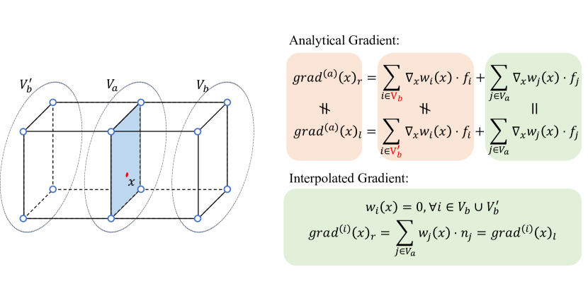
Figure 3. Gradient continuity on junction surface. A point ${\boldsymbol{x}}$ lies on the junction surface of two adjacent cubes. $V_{a}$ is the set of points on the junction surface while $V_{b}$ and $V_{b}^{\prime}$ are the sets of points outside the junction surface. As for analytical gradient at ${\boldsymbol{x}}$, the $grad^{(a)}_{r}$ from cube $V_{a}\bigcup V_{b}$ is not agree with the $grad^{(a)}_{l}$ from cube $V_{a}\bigcup V_{b}^{\prime}$, showing discontinuity. As for interpolated gradient at ${\boldsymbol{x}}$, as the weight of $V_{b}$ and $V_{b}^{\prime}$ is zero, the $grad^{(i)}_{r}$ is agree with $grad^{(i)}_{l}$, showing continuity.

4. Approach

We analyze the reasons for gradient discontinuity and solve it with interpolated gradients in Sec. 4.1, describe efficient regularization methods on the SDF grid in Sec. 4.2, geometry-radiance disentangled architecture in Sec. 4.3, and optimization details in Sec. 4.4.

4.1. SDF Gradient Interpolation

Without loss of generality, We formulate the $d$-linear interpolation on the SDF grid and derive its derivative with respect to coordinate ${\boldsymbol{x}}$. ${\boldsymbol{c}}_{i}({\boldsymbol{x}})$ is the $i$-th corner of the cube where ${\boldsymbol{x}}$ is located. $f(\cdot)$ stands for the interpolated value and $f[\cdot]$ stands for directly queried vertex value. The $d$-linear interpolation is given by Eq. 3,

(3) $$f({\boldsymbol{x}}) =\sum_{i=1}^{2^{d}}w_{i}({\boldsymbol{x}})f[{\boldsymbol{c}}_{i}({\boldsymbol{x}})]$$

$$w_{i}({\boldsymbol{x}}) =\prod_{j=1}^{d}(1-|{\boldsymbol{x}}-{\boldsymbol{c}}_{i}({\boldsymbol{x}})|_{j}),$$

where $f({\boldsymbol{x}})$ is the sum of $2^{d}$ vertex values, weighted by $w_{i}$. We define the analytical gradient of Eq. 3 with respect to ${\boldsymbol{x}}$ as $grad^{(a)}({\boldsymbol{x}})=\nabla_{\boldsymbol{x}}f({\boldsymbol{x}})$, which can be formulated as Eq. 4,

(4) $$grad^{(a)} ({\boldsymbol{x}})=\sum_{i=1}^{2^{d}}\nabla_{\boldsymbol{x}}w_{i}({\boldsymbol{x}})\cdot f[{\boldsymbol{c}}_{i}({\boldsymbol{x}})]$$

$$\frac{\partial w_{i}({\boldsymbol{x}})}{\partial{\boldsymbol{x}}_{k}}=sign ({\boldsymbol{c}}_{i}({\boldsymbol{x}})-{\boldsymbol{x}})_{k}\cdot\prod_{j\neq k}(1-|{\boldsymbol{x}}-{\boldsymbol{c}}_{i}({\boldsymbol{x}})|_{j}),$$

where $grad^{(a)}({\boldsymbol{x}})$ is the sum of $2^{d}$ vertex values, weighted by $\nabla_{\boldsymbol{x}}w_{i}({\boldsymbol{x}})\in\mathbb{R}^{d}$.

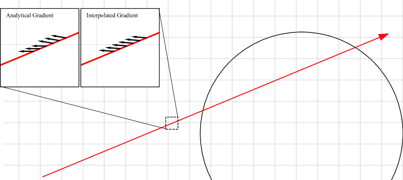
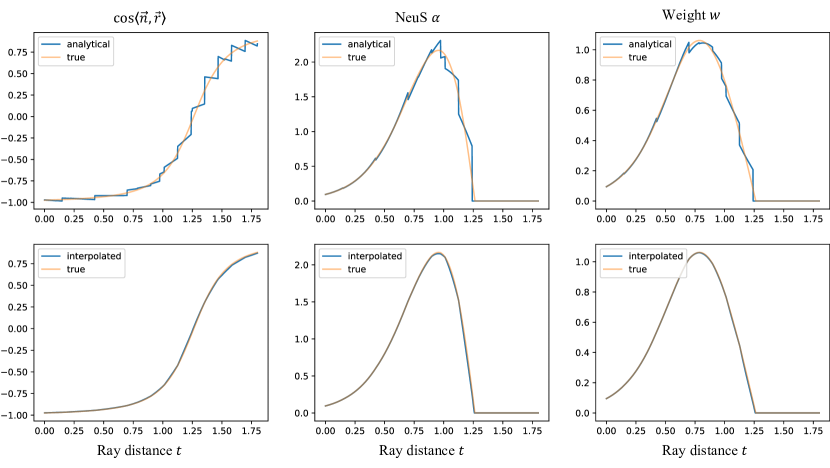
Figure 4. An 2D example to illustrate the continuity of the analytical and interpolated gradient. In this example, a ray is marching to the curved surface. The ground truth SDF values are stored on the vertices of the dense grid. The analytical gradient is computed with Eq. 4 and the interpolated gradient is computed with Eq. 7. The discontinuity of the analytical gradient can be observed at the junction surface (left). Such discontinuity causes glitches on $cos\langle{\boldsymbol{n}},{\boldsymbol{v}}\rangle$, opacity $\alpha$, and volume rendering weights $w$ (right). After applying an interpolated gradient, the estimated gradient gets close to ground truth and the glitches are eliminated.

Then, we analyse the continuity of $grad^{(a)}({\boldsymbol{x}})$ on the junction surface of adjacent cubes. Consider a point ${\boldsymbol{x}}$ lies on the junction surface. Here we assume the junction surface is the little end of the first dimension, i.e. ${\boldsymbol{x}}_{1}=\lfloor{\boldsymbol{x}}\rfloor_{1}$. Next, we split the corners into 2 groups: $V_{a}=\left\{{\boldsymbol{c}}_{i}({\boldsymbol{x}})|{\boldsymbol{c}}_{i}({\boldsymbol{x}})_{1}={\boldsymbol{x}}_{1}\right\}$ and $V_{b}=\left\{{\boldsymbol{c}}_{i}({\boldsymbol{x}})|{\boldsymbol{c}}_{i}({\boldsymbol{x}})_{1}={\boldsymbol{x}}_{1}+1\right\}$. $V_{a}$ are on the junction surface while $V_{b}$ are not. $grad^{(a)}({\boldsymbol{x}})$ is the weighted sum of the values of vertices in $V_{a}$ and $V_{b}$. The weights of vertices in $V_{b}$, i.e. $\left\{\nabla_{\boldsymbol{x}}w_{i}({\boldsymbol{x}})|{\boldsymbol{c}}_{i}({\boldsymbol{x}})\in V_{b}\right\}$, given by Eq. 5,

(5) $$\nabla_{\boldsymbol{x}}w_{i}({\boldsymbol{x}})=\left[\prod_{j=2}^{d}(1-|{\boldsymbol{x}}-{\boldsymbol{c}}_{i}({\boldsymbol{x}})|_{j}),\textbf{0}^{(d-1)}\right]^{T},$$

$$where\quad{\boldsymbol{c}}_{i}({\boldsymbol{x}})\in V_{b}$$

is non-zero, thus leading to disagreement between two adjacent cubes. Therefore, $grad^{(a)}({\boldsymbol{x}})$ is not continuous on the junction surface. A more intuitive illustration can be found in Fig. 3.

According to the NeuS volume rendering scheme in Eq. 2, the discontinuity of gradient results in the fluctuation of opacity $\alpha_{i}$ and further affects the volume rendering. An example in 2D is shown in Fig. 4, where a ray hits a curved surface. Discontinuous gradients lead to fluctuations in the curves of cosine, opacity and weight.

Based on the observations above, gradient continuity is critical to NeuS optimization. We propose to replace the analytical gradient with an interpolated gradient to ensure gradient continuity. Specifically, analogous to the interpolation of SDF values, we perform the interpolation of the gradient, which is estimated through central finite differences, so that the gradient becomes continuous. In 3D space, the estimated vertex gradient ${\boldsymbol{n}}[x,y,z]$ is given by Eq. 6:

(6) $$\frac{\partial f[x,y,z]}{\partial x} =(f[x+1,y,z]-f[x-1,y,z])/2\epsilon,$$

$$\frac{\partial f[x,y,z]}{\partial y} =(f[x,y+1,z]-f[x,y-1,z])/2\epsilon,$$

$$\frac{\partial f[x,y,z]}{\partial z} =(f[x,y,z+1]-f[x,y,z-1])/2\epsilon,$$

$${\boldsymbol{n}}[x,y,z] =\left(\frac{\partial f[x,y,z]}{\partial x},\frac{\partial f[x,y,z]}{\partial y},\frac{\partial f[x,y,z]}{\partial z}\right).$$

Then, the interpolated gradient $grad^{(i)}({\boldsymbol{x}})$ is defined by Eq. 7,

(7) $$grad^{(i)}({\boldsymbol{x}})=\sum_{i=1}^{2^{d}}w_{i}({\boldsymbol{x}}){\boldsymbol{n}}[{\boldsymbol{c}}_{i}({\boldsymbol{x}})].$$

Similarly, we analyse the continuity of $grad^{(i)}({\boldsymbol{x}})$ in Eq. 7. The weights of vertices in $V_{b}$, i.e. $\left\{w_{i}({\boldsymbol{x}})|{\boldsymbol{c}}_{i}({\boldsymbol{x}})\in V_{b}\right\}$ is given by:

(8) $$w_{i}({\boldsymbol{x}})=\prod_{j=1}^{d}(1-|{\boldsymbol{x}}-{\boldsymbol{c}}_{i}({\boldsymbol{x}})|_{j})=\textbf{0},$$

$$where\quad{\boldsymbol{c}}_{i}({\boldsymbol{x}})\in V_{b}$$

which means that the interpolated gradient $grad^{(i)}({\boldsymbol{x}})$ is continuous at the junction surface. As shown in Fig. 4, the interpolated gradient eliminates the fluctuations of volume rendering weights.

4.2. Efficient SDF Regularization

In VoxNeuS, we apply Eikonal loss (Gropp et al., 2020) and curvature loss (Li et al., 2023) to SDF dense grids. The regularization is not applied to the interpolated points but the vertices of the grid. This design achieves the same regularization effect while avoiding interpolation, thereby improving efficiency.

Specifically, the vertices set for regularization is given by Eq.9:

(9) $$V_{R}=\left\{{\boldsymbol{c}}_{i}({\boldsymbol{x}})|i=1,...,2^{d};{\boldsymbol{x}}\in\mathcal{B}\right\}$$

where $\mathcal{B}$ is the sampled points on the batch of rays for volume rendering. The vertices in $V_{R}$ are uniformly regularized.

Current learning framework, like PyTorch, supports automatic differentiation. However, when handling the regularization term on vertices set $V_{R}$, frequent unstructured memory access makes it a bottleneck. To accelerate this computation, we take advantage of the explicit representation of SDF values to directly solve for the gradient of the regularization term. These manually solved gradients will be added to the gradient obtained by automatic differentiation, i.e. $\boldsymbol{\mathcal{G}}\leftarrow\boldsymbol{\mathcal{G}}+w_{eik}\boldsymbol{\mathcal{G}}_{eik}+w_{curv}\boldsymbol{\mathcal{G}}_{curv}$.

The Eikonal loss function makes the learned field satisfy the SDF property (Barrett and Dherin, 2020). Its formulation and derivative with respect to finite difference $n[x]$ are given by Eq. 10:

(10) $$\mathcal{L}_{eik}=\frac{1}{|V_{R}|}\sum_{{\boldsymbol{x}}\in V_{R}}(||{\boldsymbol{n}}[{\boldsymbol{x}}]||_{2}-1)^{2}$$

$$\frac{\partial\mathcal{L}_{eik}}{\partial{\boldsymbol{n}}[{\boldsymbol{x}}]}=\frac{1}{|V_{R}|}(1-||{\boldsymbol{n}}[{\boldsymbol{x}}]||_{2}^{-1}).$$

The derivative of ${\boldsymbol{n}}[{\boldsymbol{x}}]$ with respect to ${\boldsymbol{x}}$’s neighbourhood SDF values $f[U({\boldsymbol{x}})]$ can be derived from Eq. 6. Combining it with Eq. 10, the $\mathcal{G}_{eik}$ is formulated as:

(11) $$\boldsymbol{\mathcal{G}}_{eik}=\sum_{{\boldsymbol{x}}\in V_{R}}\frac{\partial\mathcal{L}_{eik}}{\partial{\boldsymbol{n}}[{\boldsymbol{x}}]}\cdot\frac{\partial{\boldsymbol{n}}[{\boldsymbol{x}}]}{\partial f[U({\boldsymbol{x}})]}.$$

We penalize the mean squared curvature of SDF to encourage smoothness. The curvature is computed from discrete Laplacian, as given by Eq. 12 ($d=3$).

(12) $$\nabla^{2}f[x,y,z]=\frac{1}{\epsilon^{2}}\left[\begin{aligned} f[x+1,y,z]+f[x-1,y,z]-2f[x,y,z]\\ f[x,y+1,z]+f[x,y-1,z]-2f[x,y,z]\\ f[x,y,z+1]+f[x,y,z-1]-2f[x,y,z]\\ \end{aligned}\right]$$

The curvature loss and its derivative are defined as Eq. 13,

(13) $$\mathcal{L}_{curv}= \frac{1}{|V_{R}|}\sum_{{\boldsymbol{x}}\in V_{R}}||\nabla^{2}f[{\boldsymbol{x}}]||^{2}_{2}$$

$$\boldsymbol{\mathcal{G}}_{curv}=\frac{2}{|V_{R}|} \sum_{{\boldsymbol{x}}\in V_{R}}\nabla^{2}f[{\boldsymbol{x}}]\cdot\frac{\partial\nabla^{2}f[{\boldsymbol{x}}]}{\partial f[U({\boldsymbol{x}})]}.$$

While larger curvature weight $w_{curv}$ encourages smoothness, it hinders the initial convergence and later detail optimization (Li et al., 2023). Therefore dedicated scheduling is applied: $w_{curv}$ is a small constant at first, linearly increases at the following stage, and exponentially decreases at the final stage.

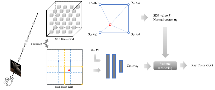
Figure 5. Network architecture overview.

4.3. Network Architecture

In volume rendering, geometry and radiance are handled in two independent passes, merged when blending the sampled points (Eq. 1). However, general implementations adopt the same network for the prediction of both radiance and geometry. Such an entanglement lets the optimization of radiance pass affect the geometry. The problem appears when rendering a textured plane, as shown in Fig. 6, where the plane is slightly deformed to fit the texture. Though Voxurf (Wu et al., 2022) uses two separate DVGO (Sun et al., 2022) grids as its architecture, the feature branch of dual color network predicts the point color based on local SDF values, causing the geometry to be optimized through the color prediction pass.

Based on the observations above, we adopt a geometry-radiance disentangled architecture, where the geometry is explicitly represented with an SDF dense grid and the radiance is parameterized with an iNGP hash grid, as shown in Fig. 5. Following IDR (Yariv et al., 2020), the normal is passed to the iNGP’s shallow MLP, which leads to slight optimization of geometry through radiance pass. However, no artifacts in the textured plane are observed.

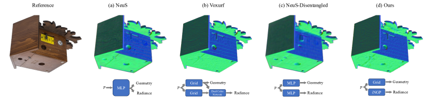
Figure 6. An illustration of geometry-radiance entanglement in volume rendering. In this example, the woodgrain roof and side stickers should be reconstructed as a plane. (a) NeuS uses one MLP to parameterize both geometry and radiance, causing geometry deformation when optimizing radiance. (b) Voxurf uses separate models to parameterize geometry and radiance. However, dual color networks use local geometry to predict radiance, resulting in two sets of parameters re-entangled. Using color cues to assist geometry optimization can improve reconstruction quality to some extent, but can also lead to artifacts in this example. (c) We modify NeuS to use independent models to parameterize geometry and color. The roof and stickers are reconstructed correctly, but the reconstruction quality is degraded. (d) Our VoxNeuS, where geometry is explicitly represented with a dense SDF grid and radiance are parameterized with an iNGP hash grid, correctly reconstructed the textured plane and improved the quality and efficiency.

4.4. Optimization Details

We describe optimization details, and implementations to improve efficiency in this section.

In VoxNeuS, we leverage a progressive super-resolution of the SDF grid to balance the coarse shape and fine detail. A small SDF dense grid is used at the beginning to initialize a coarse geometry and scaled up during training to capture details. The final resolution is $320^{3}$. Following (Yariv et al., 2023), we manually schedule the $s$ value in $\Phi_{s}$ (Eq. 2) for more accurate surface location. Specifically, the gradient $\nabla_{s}\mathcal{L}$ is amplified by $k$ times when negative (towards convergence), as formulated in Eq. 14,

(14) $$\nabla_{s}\mathcal{L}\leftarrow\left\{\begin{aligned} k\nabla_{s}\mathcal{L}\quad&\nabla_{s}\mathcal{L}<0\\ \nabla_{s}\mathcal{L}\quad&\nabla_{s}\mathcal{L}>=0,\end{aligned}\right.$$

where we set $k=5$ for all our experiments.

As the regularization term is handled by explicit gradient accumulation (Sec. 4.2), we only perform the RGB and optional mask supervision, as shown in Eq. 15,

(15) $$\mathcal{L}=\mathcal{L}_{RGB}+w_{mask}\mathcal{L}_{mask}.$$

Between the back-propagation of $\mathcal{L}$ and gradient descent, the regularization gradients (Eq.10 & 13) need to be added. After training, an optional Gaussian filtering can be applied for smoothness (Wu et al., 2022).

To further improve the computational and memory efficiency, critical operators are implemented with CUDA. For native PyTorch-based gradient interpolation, on the one hand, additional memory is required to save intermediate results for back-propagation, and on the other hand, non-local memory access results in a longer computation time. Therefore, we use CUDA to achieve local memory access, and use re-computation in backward pass to avoid the memory overhead of intermediate results. The explicit gradient computation of Eq. 10 & Eq. 13 is also implemented with CUDA for local memory access. Besides, the gradient descent introduces the multiply and add operation on the entire dense grid, which is unignorable when the resolution becomes higher. Following iNGP (Müller et al., 2022), we utilize the sparsity of gradient and only update the SDF values whose gradient is non-zero. Although this strategy violates Adam’s assumption, it does not cause a loss of precision.

5. Experiments

5.1. Experiment Setup

We evaluate our method on DTU (Jensen et al., 2014) dataset quantitatively and qualitatively, and further show qualitative results on several challenging scenes from the BlendedMVS (Yao et al., 2020). We include several baselines for comparison: 1) Colmap (Schönberger and Frahm, 2016); 2) IDR (Yariv et al., 2020); 3) NeuS (Wang et al., 2021); 4) VolSDF (Yariv et al., 2021); 5) NeRF (Mildenhall et al., 2021); 6) Voxurf (Wu et al., 2022); 7) NeuS2 (Wang et al., 2023a); 8) 2DGS (Huang et al., 2024). Among them, only 2) and 7) require foreground masks.

We train our models for 40k steps with ray batch size of 2048. The resolution of dense SDF grid is set to $96^{3}$ at beginning, scaling to $160^{3}$ after 10k steps, and scaling to $320^{2}$ after next 20k steps. We set the Eikonal weight $w_{eik}=10^{-2}$ for first 11k steps, linearly decrease to $10^{-3}$ for the next 10k steps. We set the curvature weight $w_{curv}=10^{-8}$ for the first 11k steps, linearly increase to $5\times 10^{-6}$ for the next 10k steps, and exponentially decrease to $5\times 10^{-7}$ during the remaining steps.

5.2. Comparative Study

We report the quantitative results for surface reconstruction without foreground supervision on the DTU dataset on Tab. 2. The results show that our method achieves a lower Chamfer Distance than previous methods under the same setting. We conduct a qualitative evaluation on DTU and BlendedMVS datasets respectively, without the supervision of foreground masks, as shown in Fig. 7. NeuS achieves a relatively smooth surface, but loses some high-frequency information, and the normal estimate with MLP derivatives is inaccurate. NeuS2 and Voxurf improve high-frequency details, but the surface is rough. All comparison methods are affected by surface texture when reconstructing planes, resulting in deformation. In comparison, our method obtains a smoother surface while retaining high-frequency details due to the gradient interpolation and geometry-radiance disentanglement.

We further compare the efficiency and performance with our main baselines Voxurf (Wu et al., 2022) and NeuS2 (Wang et al., 2023a), as shown in Tab. 3. NeuS2 and our method are evaluated on 2080ti while Voxurf is evaluated on RTX 3090 to meet its memory consumption. Voxurf’s two-stage training policy and complicated strategy make it computational and memory inefficient. NeuS2 implements the whole system in CUDA to avoid the computational overhead that the learning framework introduces, and directly calculates second-order derivatives for acceleration. Thus the 20k iterations of training cost 9 minutes and 6.2 GB of memory, but with the sacrifice of flexibility. Our method is mainly implemented in Python, and only key operators are accelerated using CUDA. Compared with NeuS2, the iterations of VoxNeuS are doubled, because the geometry-radiance disentangled architecture requires longer iterations to converge. Even so, VoxNeuS can still complete training in 15 minutes while using only 2.5 GB of memory. As for performance, VoxNeuS achieves the best novel-view PSNR and Chamfer Distance. NeuS2 is not applicable without foreground masks.

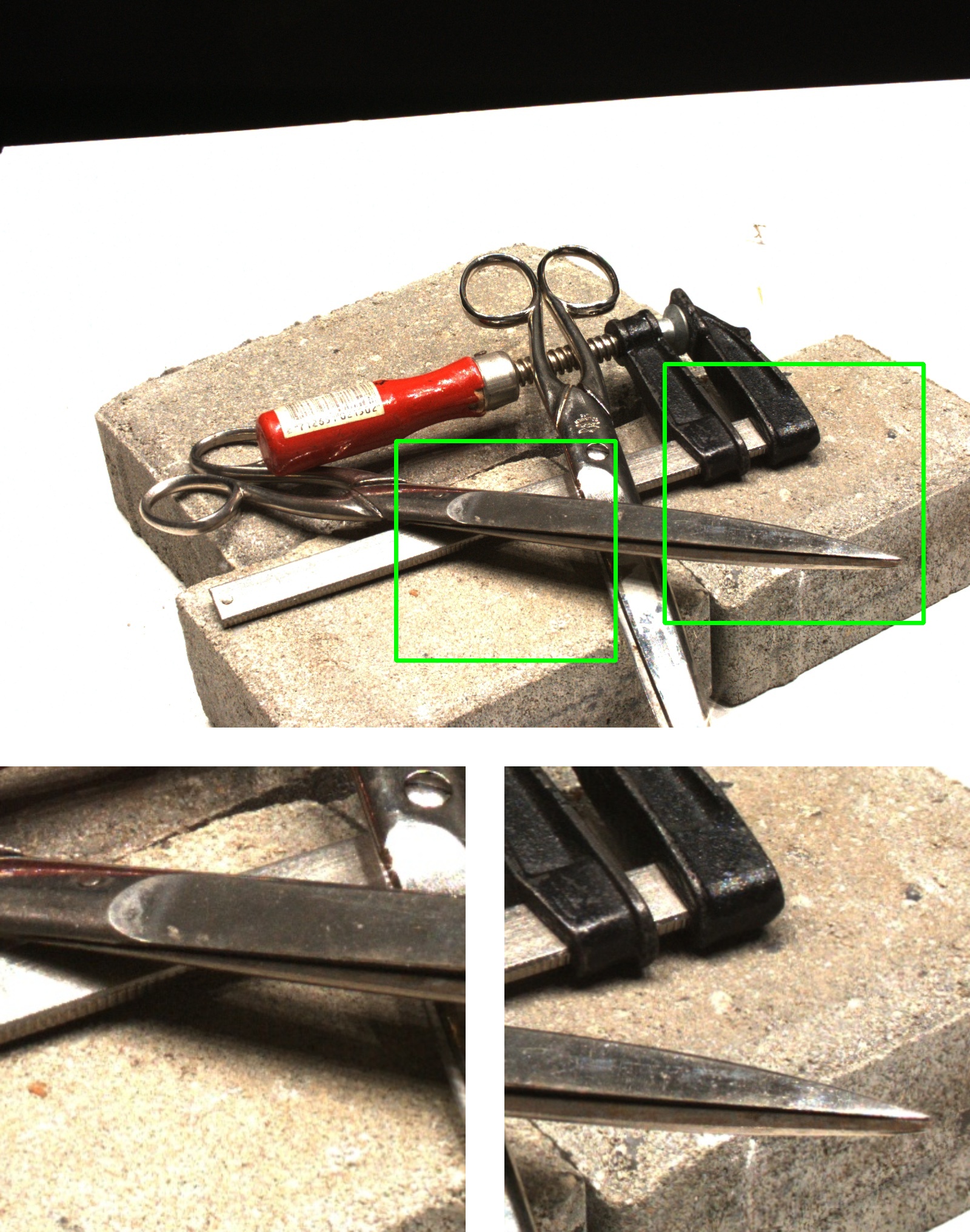
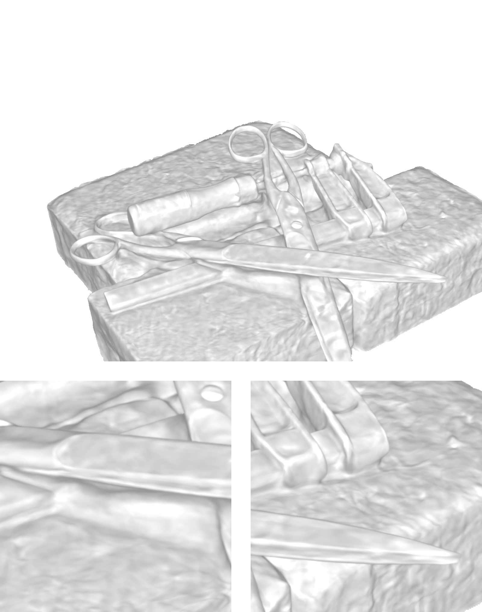
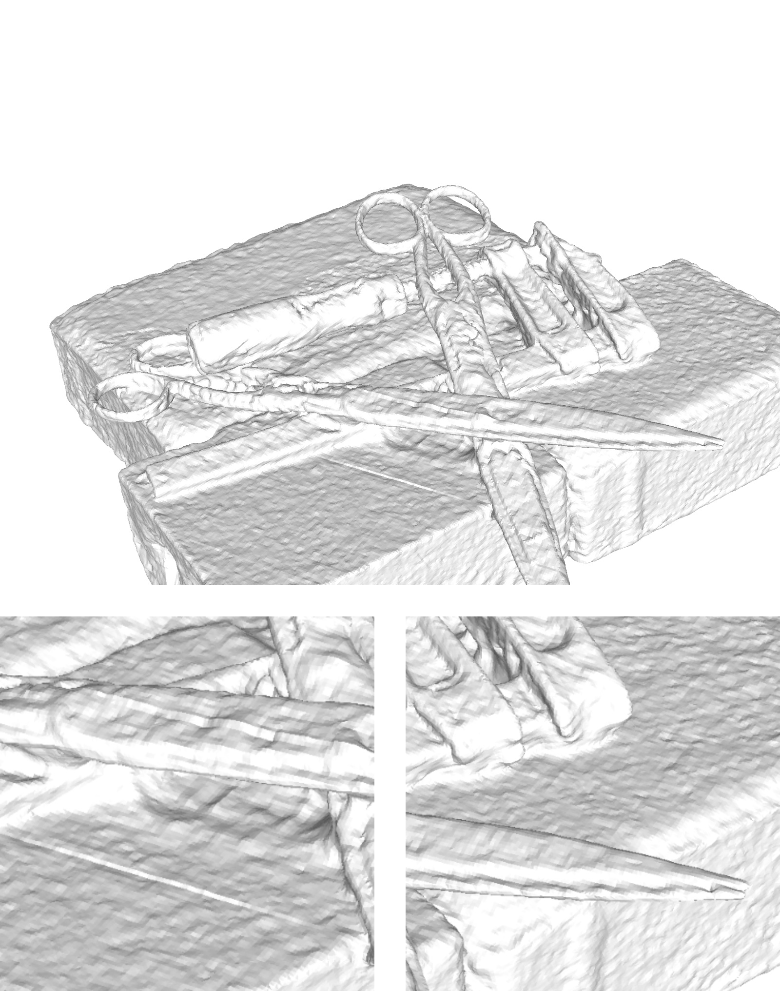
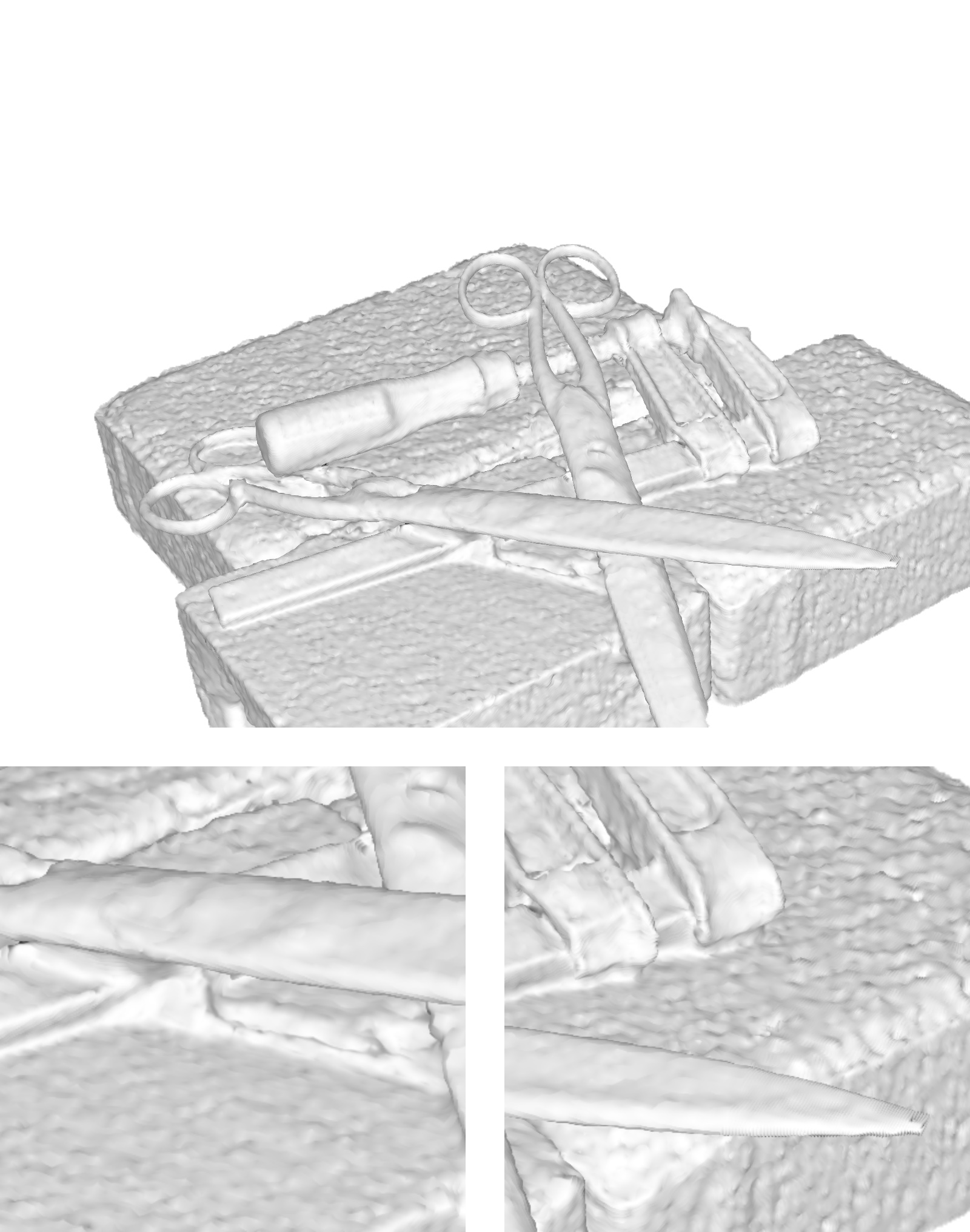
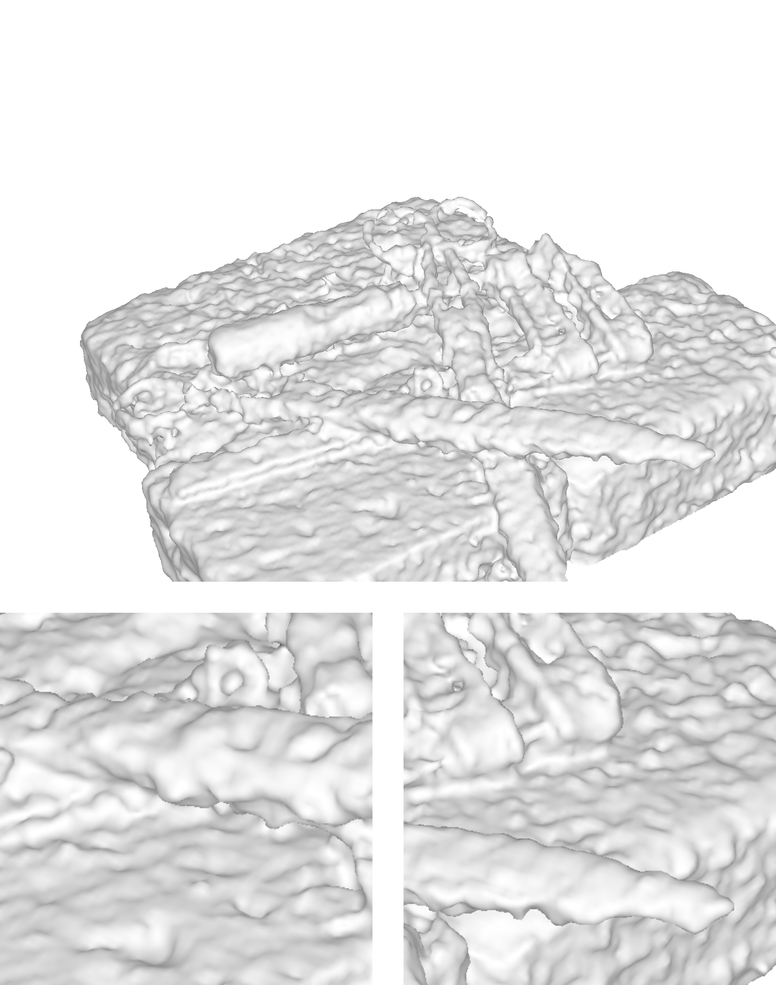
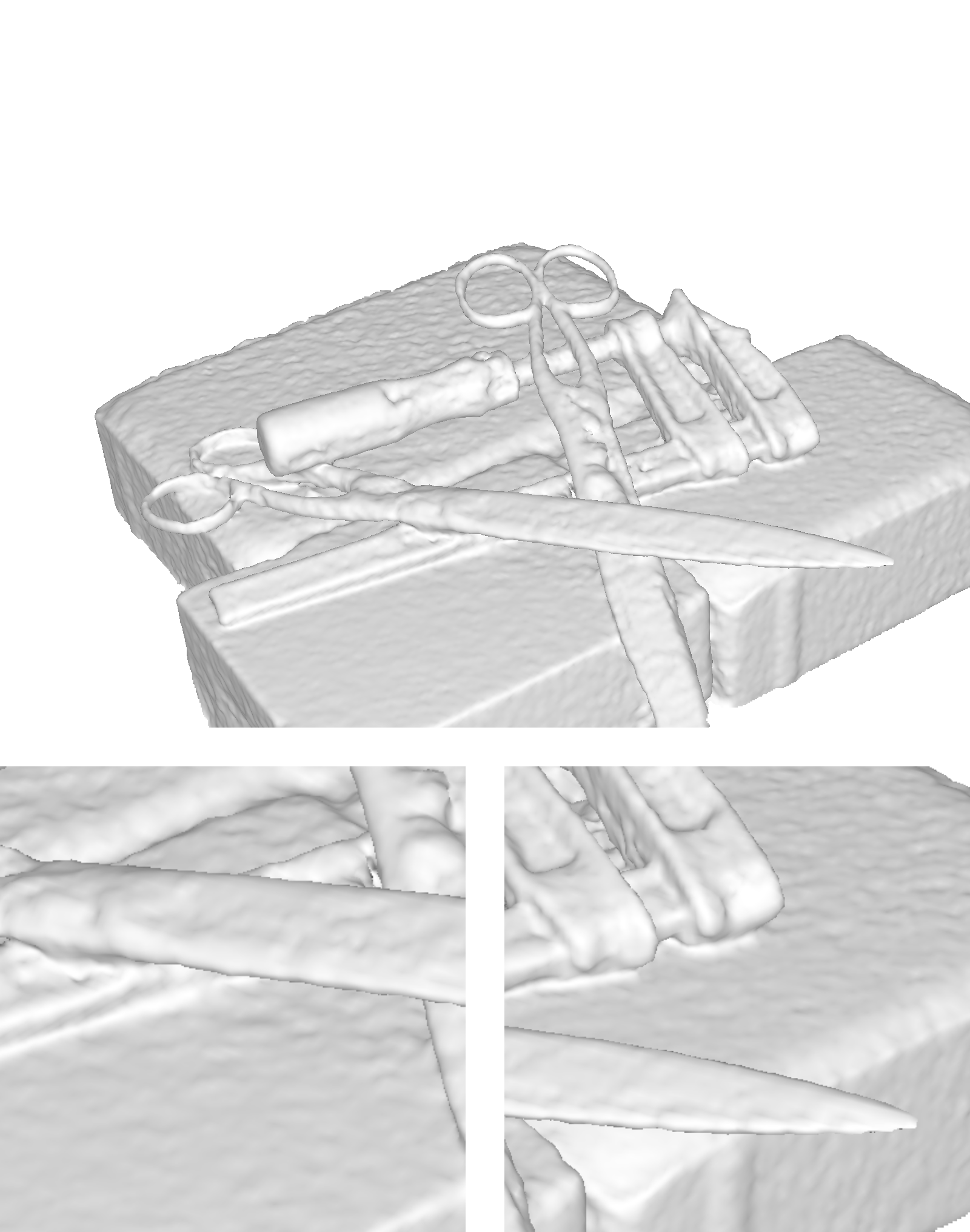
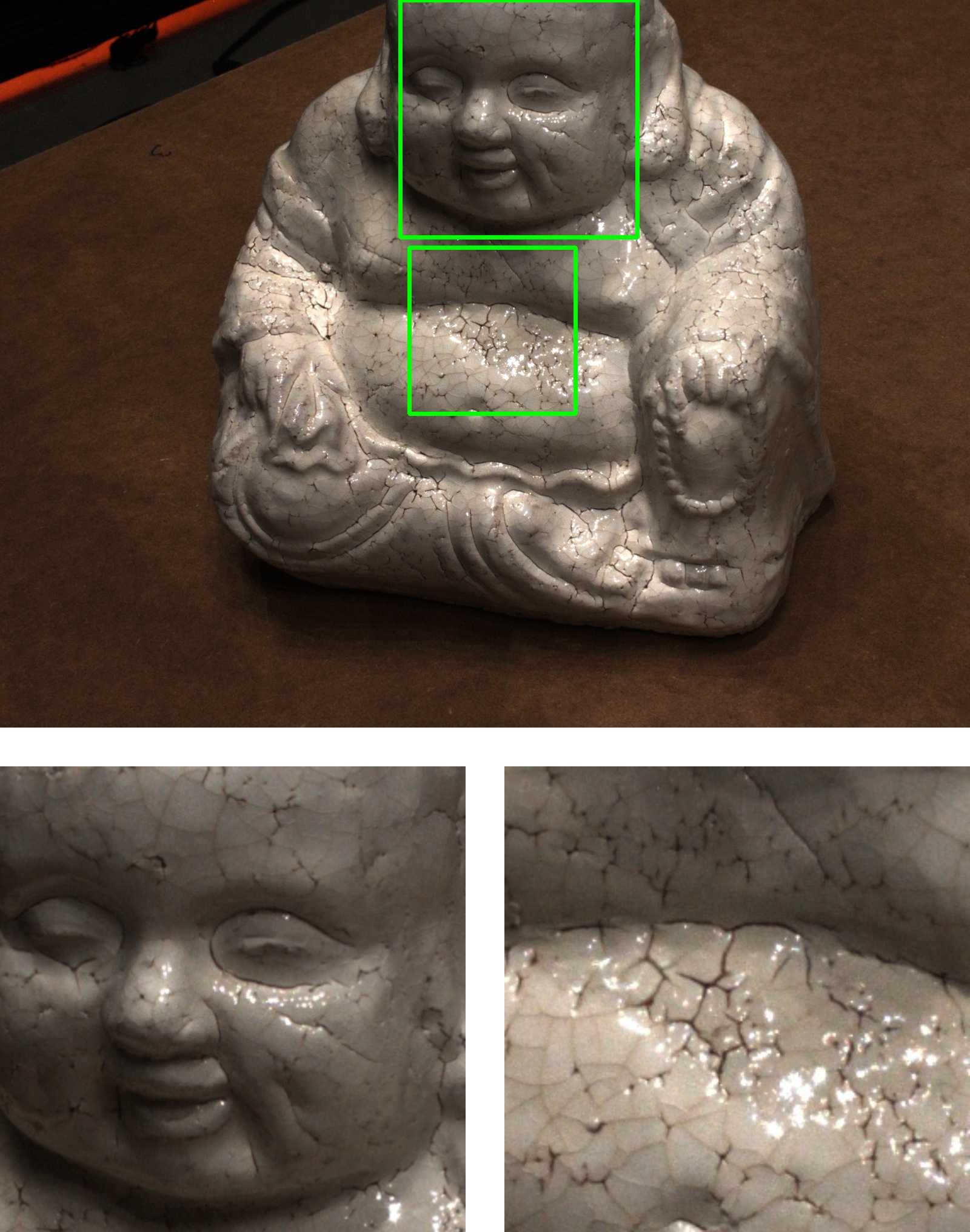
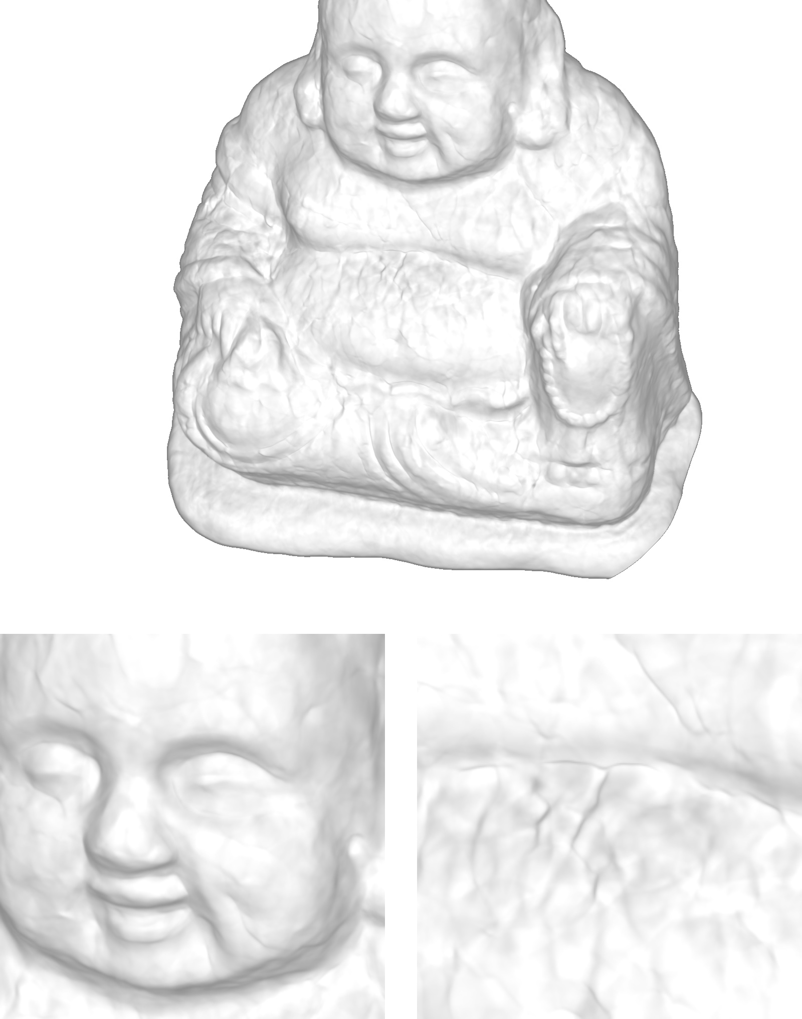
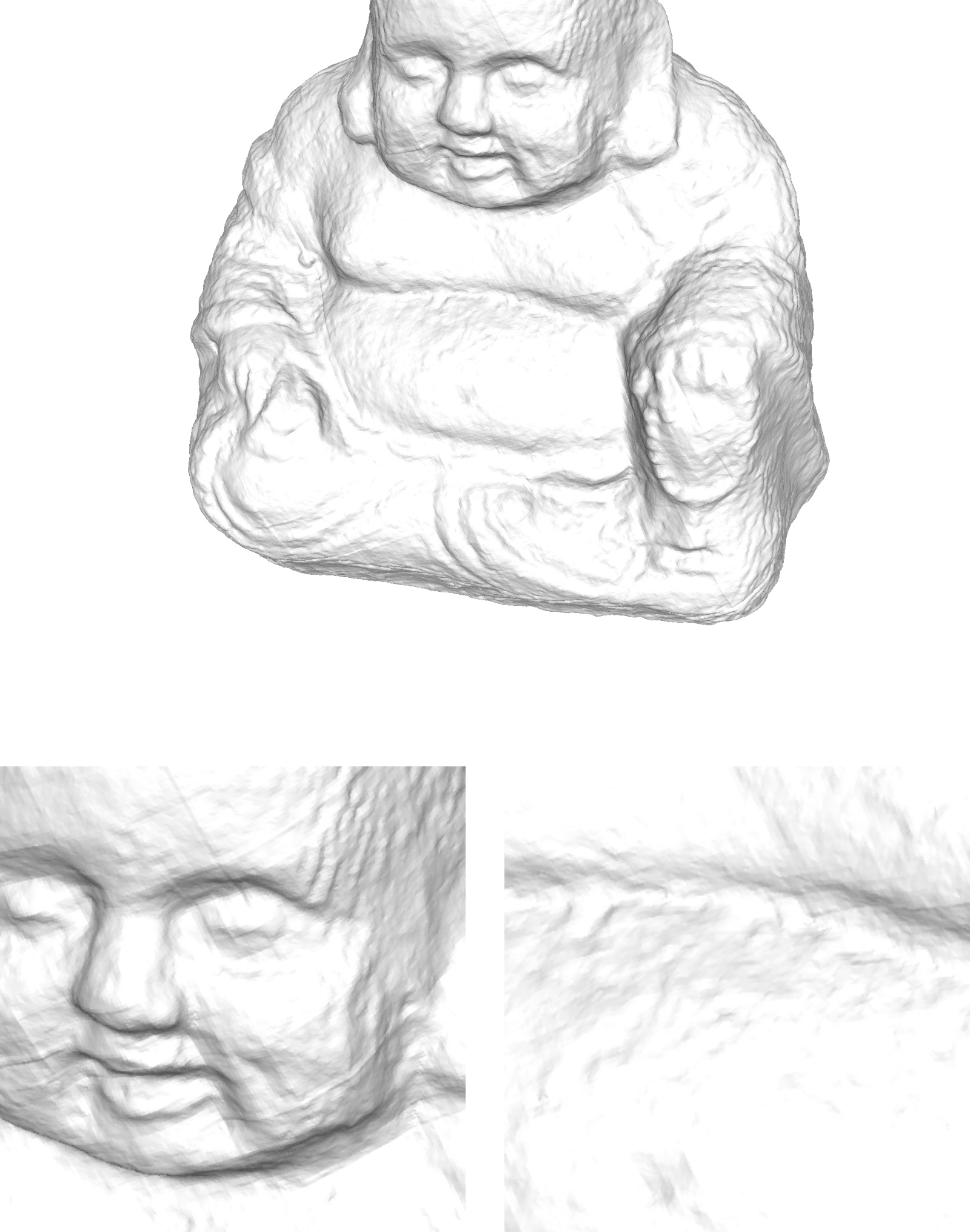
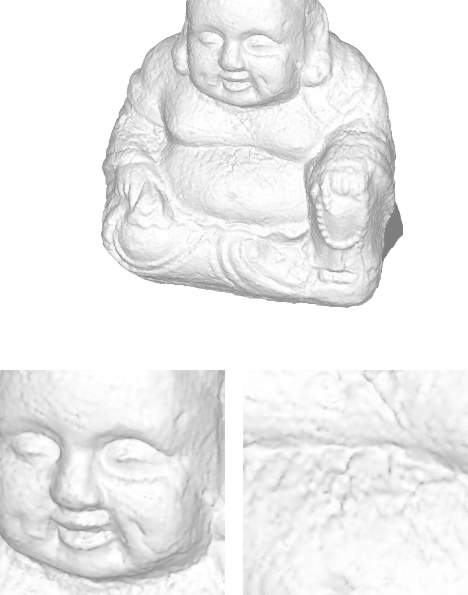
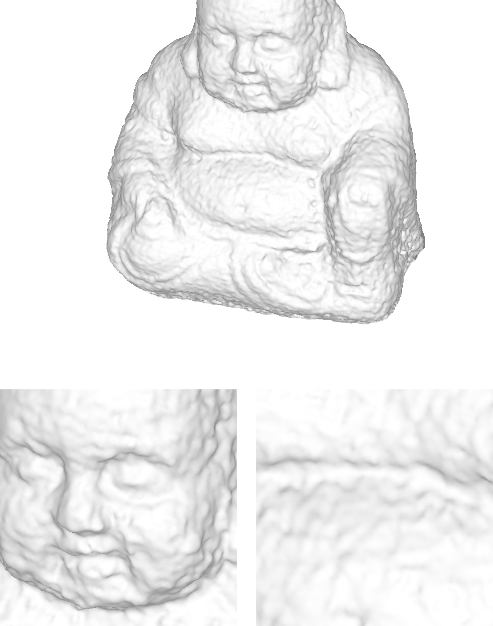
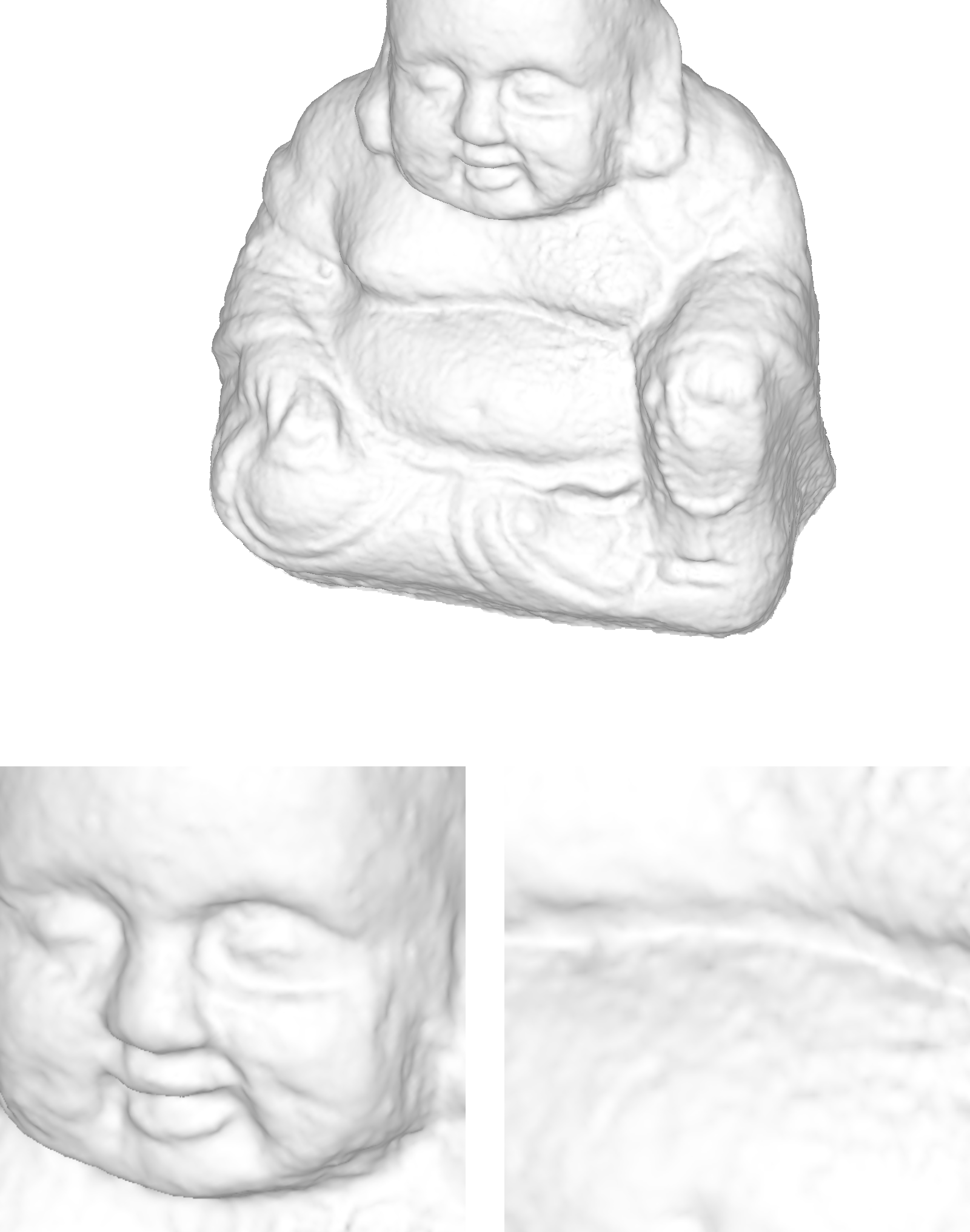
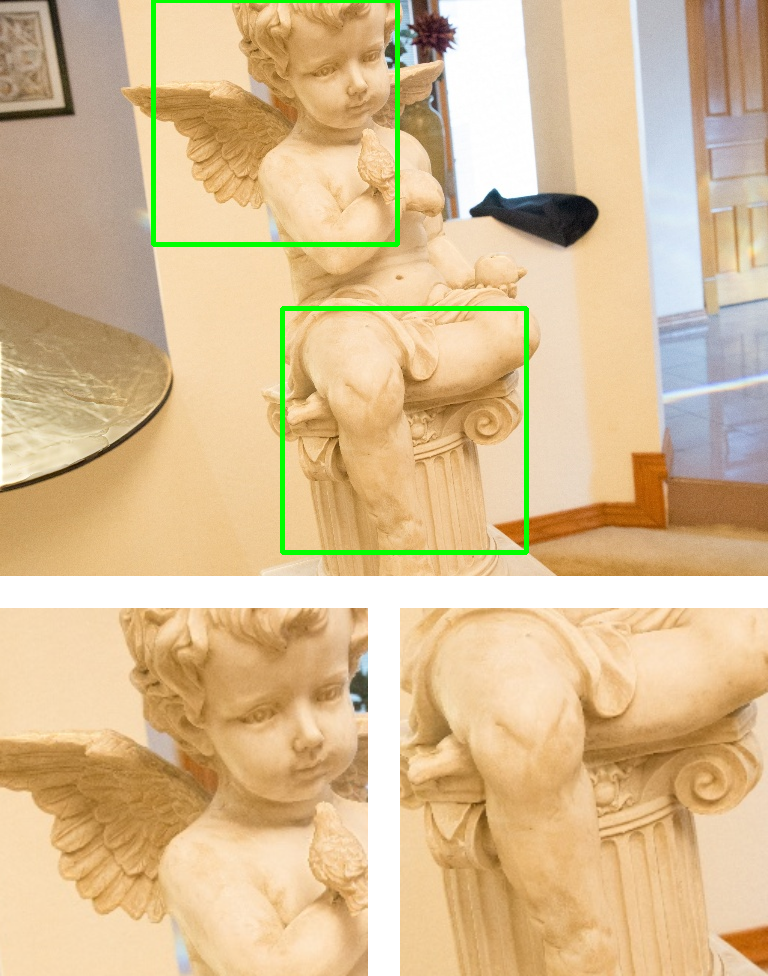
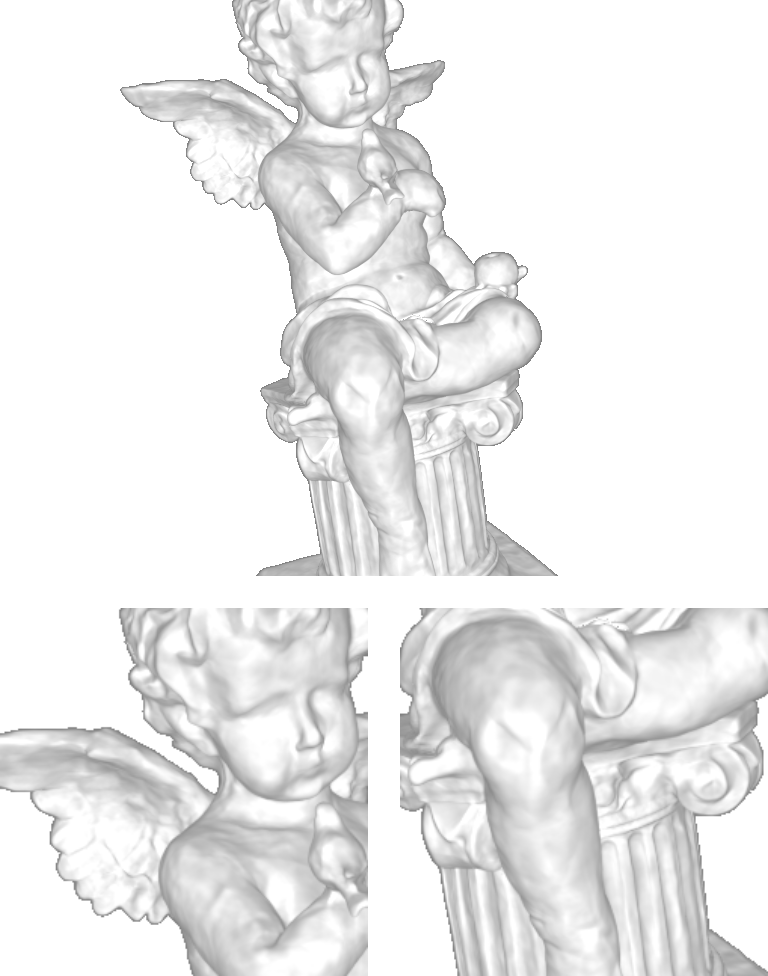
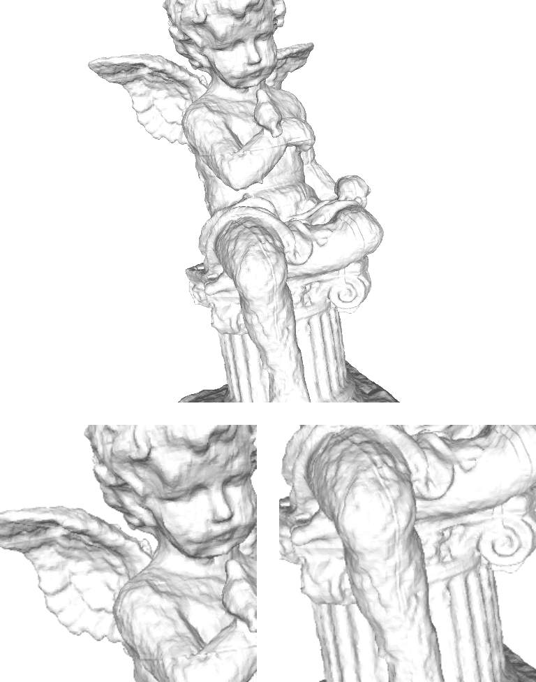
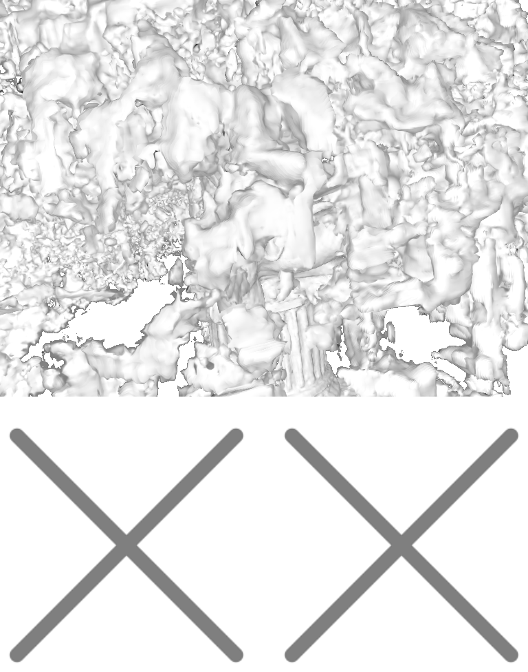
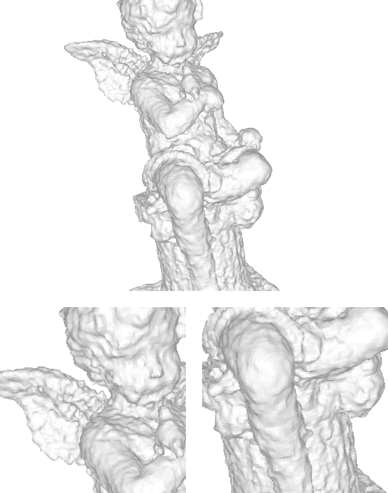
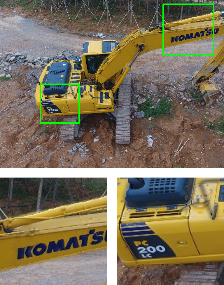
(a) Ground Truth

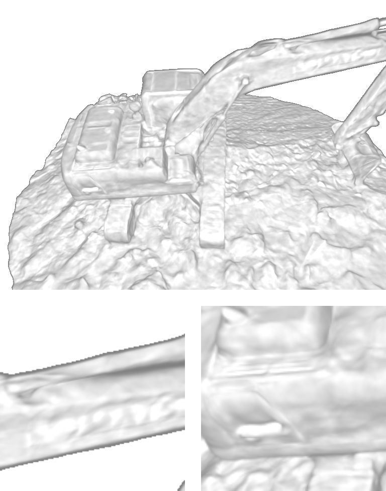
(b) NeuS

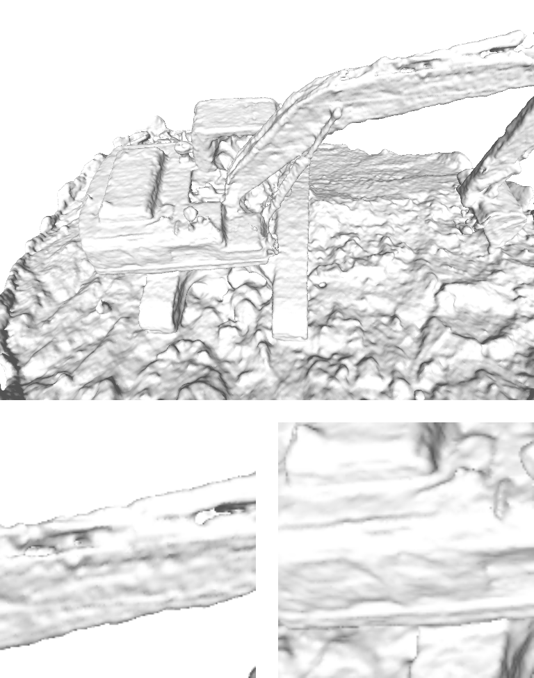
(c) NeuS2

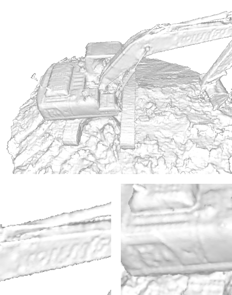
(d) Voxurf

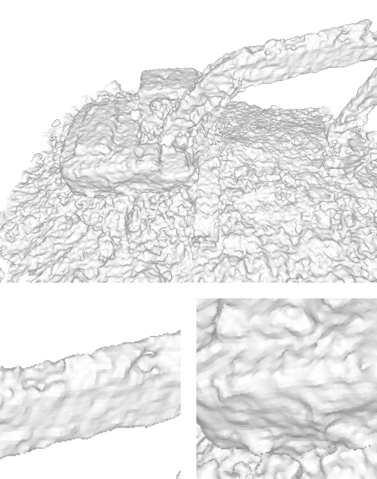
(e) w/o Interp. Grad.

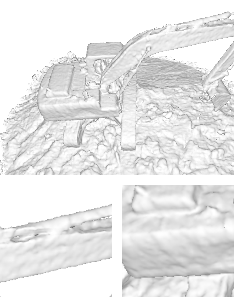
(f) Ours

Figure 7. Visual comparison among different methods. All methods except NeuS2 (Wang et al., 2023a) are trained without foreground masks. The first two cases are from DTU (Jensen et al., 2014), while the next two are from BlendedMVS (Yao et al., 2020). Voxurf failed to reconstruct the 3rd case due to the inability to distinguish foreground and foreground.

5.3. Ablation Study

Table 1. Ablation study on gradient interpolation.

Gradient	Analytical	Interpolated
w/o mask	0.93	0.72
w/ mask	0.82	0.70

Table 2. Comparison among different methods without foreground mask supervision. The best and second best results are marked with bold and underline respectively.

Scan	24	37	40	55	63	65	69	83	97	105	106	110	114	118	122	mean
NeRF(Mildenhall et al., 2021)	1.90	1.60	1.85	0.58	2.28	1.27	1.47	1.67	2.05	1.07	0.88	2.53	1.06	1.15	0.96	1.49
Colmap(Yu et al., 2022)	0.81	2.05	0.73	1.22	1.79	1.58	1.02	3.05	1.40	2.05	1.00	1.32	0.49	0.78	1.17	1.36
VolSDF(Yariv et al., 2021)	1.14	1.26	0.81	0.49	1.25	0.70	0.72	1.29	1.18	0.70	0.66	1.08	0.42	0.61	0.55	0.86
NeuS(Wang et al., 2021)	1.00	1.37	0.93	0.43	1.10	0.65	0.57	1.48	1.09	0.83	0.52	1.20	0.35	0.49	0.54	0.84
2DGS(Huang et al., 2024)	0.48	0.91	0.39	0.39	1.01	0.83	0.81	1.36	1.27	0.76	0.70	1.40	0.40	0.76	0.52	0.80
Voxurf(Wu et al., 2022)	0.72	0.75	0.47	0.39	1.47	0.76	0.81	1.02	1.04	0.92	0.52	1.13	0.40	0.53	0.53	0.76
Ours	0.58	0.76	0.40	0.36	1.09	0.76	0.70	1.29	1.15	0.84	0.44	1.02	0.42	0.50	0.49	0.72

Table 3. Comparison on efficiency and performance among Voxurf (Wu et al., 2022), NeuS2 (Wang et al., 2023a), and our method.

Methods	Batches/s	Training Time	GPU Memory	Implementation	PSNR	CD w/ mask	CD w/o mask
NeuS	8.3	10 hours	10 GB	Python	29.63	0.77	0.84
Voxurf	10.0	50 mins	14 GB	Python & CUDA/C++	32.16	0.72	0.76
NeuS2	37.0	9 mins	6.2 GB	CUDA/C++	32.14	0.70	-
Ours	44.4	15 mins	2.5 GB	Python & CUDA/C++	32.21	0.70	0.72

This section evaluates our method’s effectiveness in gradient interpolation and regularization terms.

We first evaluate the effectiveness of interpolated gradient on the DTU dataset with Chamfer Distance. The quantitative results are listed in Tab 1. All hyper-parameters are kept the same except for the estimation strategy of the SDF gradient $\nabla_{\boldsymbol{x}}f({\boldsymbol{x}})$. Some qualitative comparison is shown in Fig. 2 and Fig. 7. Experimental results show that gradient interpolation is key to the correct reconstruction of our method. The glitches (Fig.4) caused by the analytical gradient make the reconstructed surface discontinuous and rough.

Then we qualitatively evaluate the effectiveness of regularization terms, taking a scene of the DTU dataset as an example. The reconstructions without Eikonal loss or/and curvature loss are illustrated in Fig 8. Previous MLP-based implicit representation provides strong low-frequency priors, making the reconstruction smooth. However, our voxel-based explicit representation makes the regularization terms particularly important for reconstruction. Curvature loss makes the surface smooth, while Eikonal loss makes the SDF grid converge normally.

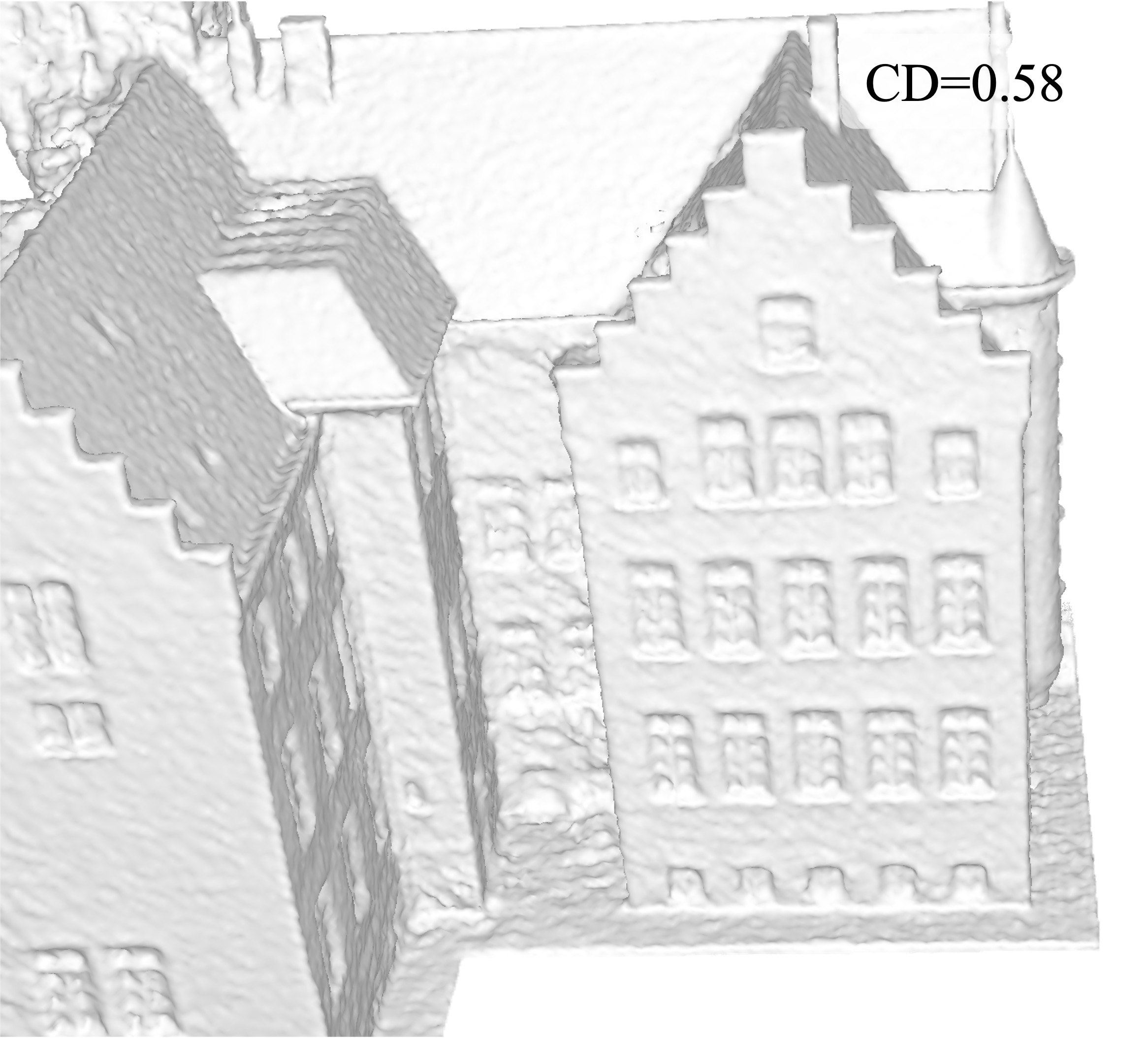
(a) full

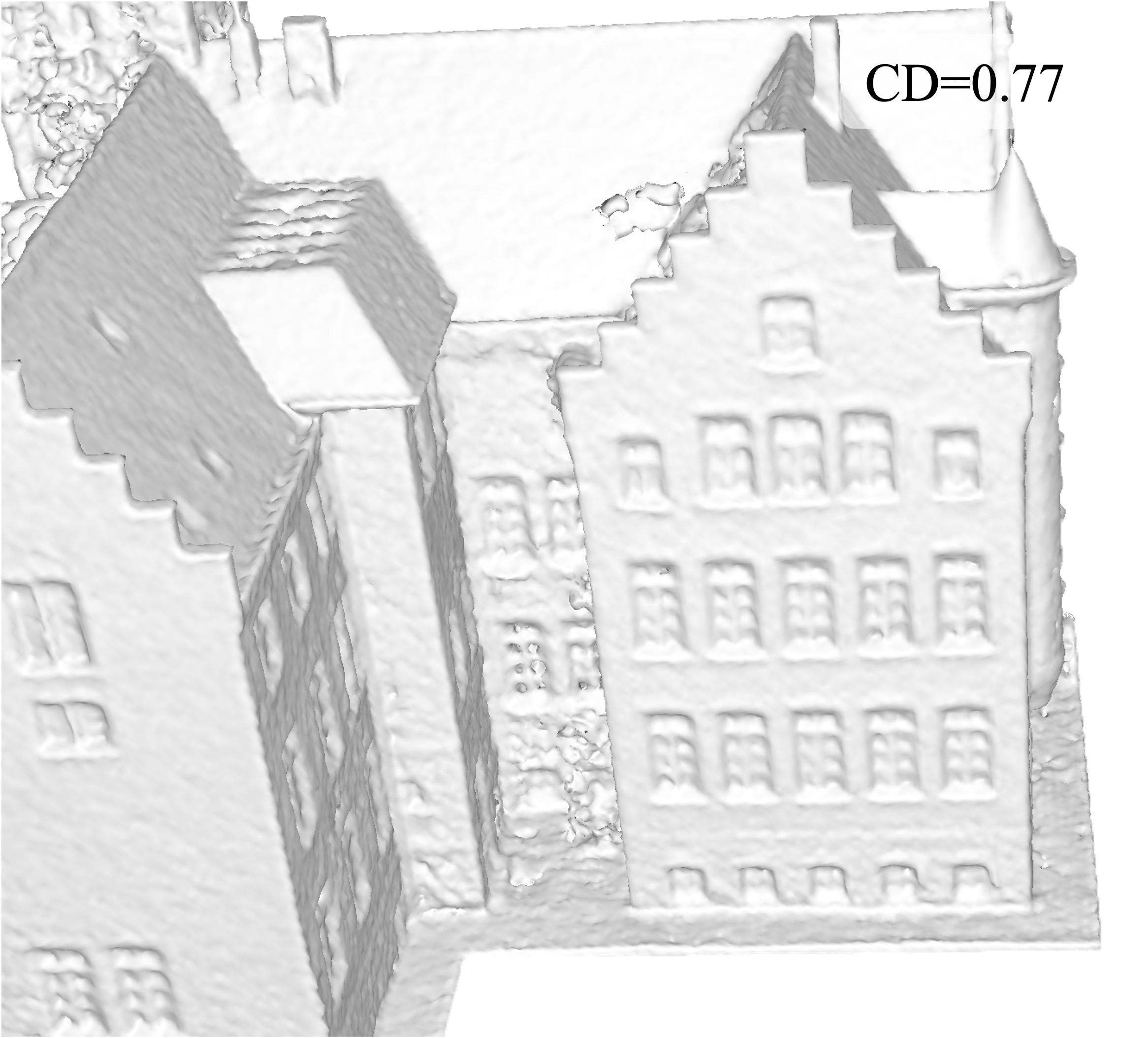
(b) w/o curvature

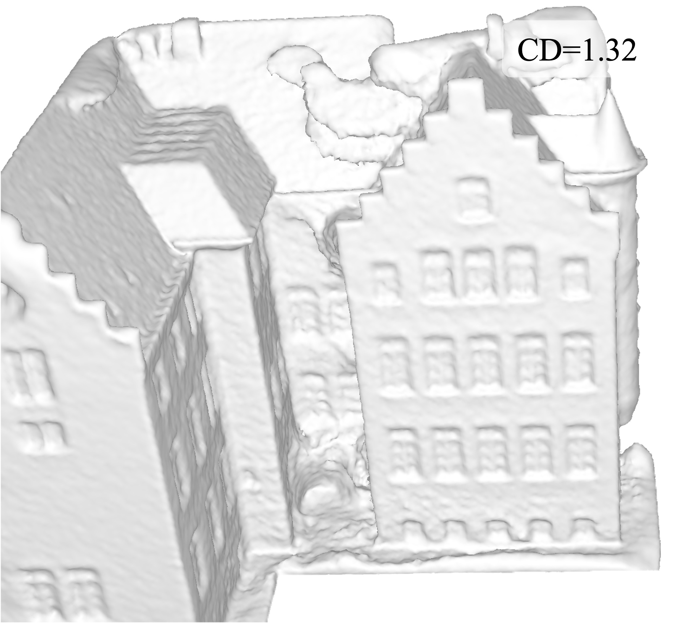
(c) w/o Eikonal

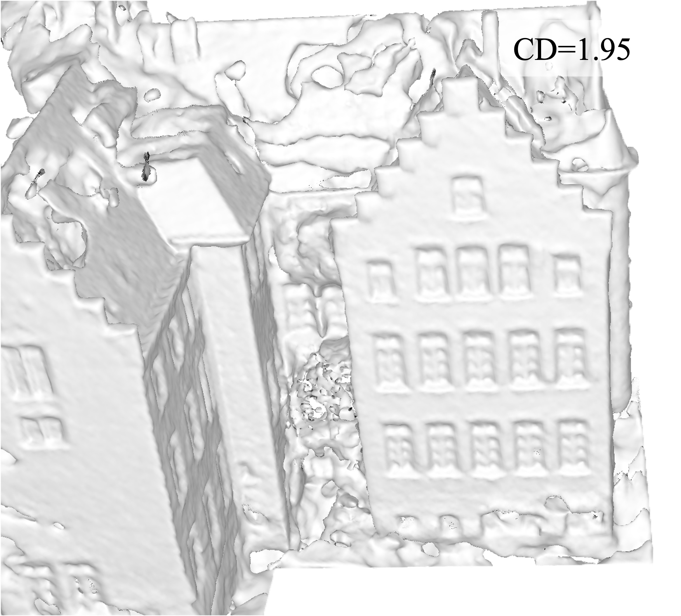
(d) w/o both

Figure 8. Ablation study on regularization terms.

5.4. Efficiency Study

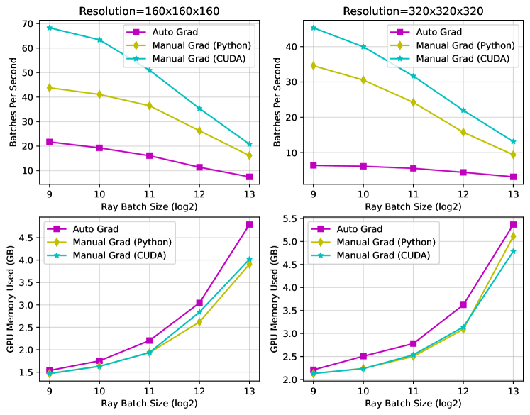
Figure 9. Comparison of speed and memory among different implementations for Eikonal and curvature regularization. Auto Grad: automatic differentiation provided by PyTorch; Manual Grad (Python): our explicit gradient solving in Python; Manual Grad (CUDA): ours in CUDA/C++.

In this experiment, we evaluate the acceleration of our efficient SDF regularization, as shown in Fig. 9. We compare the training speed and memory consumption under different regularization settings. When automatic differentiation is applied, regularization is the training bottleneck, taking up more than 70% of the training time. This is because frequent unstructured memory access leads to cache misses, which in turn affects efficiency. Our explicit gradient solving reduces the frequency of memory accesses and computations, increasing the overall training speed by 2.2x. The CUDA implementation of explicit gradient solving eliminates the overhead caused by Python and improves the locality of memory access, thus bringing about 3x acceleration and eliminating this bottleneck. We set the ray batch size as 2048 to balance performance with time and memory overhead.

6. Conclusion

We propose VoxNeuS, an efficient neural surface reconstruction method, where SDF values are explicitly stored in a dense grid to improve efficiency and model high-frequency details. However, trilinear interpolation makes the gradient discontinuous, thereby degrading the reconstruction quality. Therefore, we propose interpolated gradients to eliminate discontinuities caused by original analytical gradients. To tackle the bottleneck caused by the automatic differentiation of regularization terms, we take advantage of explicit expression, explicitly solve its derivatives and implement it using CUDA, thus optimizing the memory access frequency and locality. In terms of network architecture, we found that using the same network to fit geometry and radiance, or entangling the geometry and radiance in the computation graph, makes the geometric structure deform to fit the radiance. Therefore, we designed a geometry-radiance disentangled architecture to eliminate this artifact. The experiments illustrate the efficiency and effectiveness of our method.

References

- (1)
- Barrett and Dherin (2020) David GT Barrett and Benoit Dherin. 2020. Implicit gradient regularization. arXiv preprint arXiv:2009.11162 (2020).
- Cai et al. (2023) Bowen Cai, Jinchi Huang, Rongfei Jia, Chengfei Lv, and Huan Fu. 2023. Neuda: Neural deformable anchor for high-fidelity implicit surface reconstruction. In Proceedings of the IEEE/CVF Conference on Computer Vision and Pattern Recognition. 8476–8485.
- Darmon et al. (2022) François Darmon, Bénédicte Bascle, Jean-Clément Devaux, Pascal Monasse, and Mathieu Aubry. 2022. Improving neural implicit surfaces geometry with patch warping. In Proceedings of the IEEE/CVF Conference on Computer Vision and Pattern Recognition. 6260–6269.
- Fridovich-Keil et al. (2022) Sara Fridovich-Keil, Alex Yu, Matthew Tancik, Qinhong Chen, Benjamin Recht, and Angjoo Kanazawa. 2022. Plenoxels: Radiance fields without neural networks. In Proceedings of the IEEE/CVF Conference on Computer Vision and Pattern Recognition. 5501–5510.
- Green (2007) Chris Green. 2007. Improved alpha-tested magnification for vector textures and special effects. In ACM SIGGRAPH 2007 courses. 9–18.
- Gropp et al. (2020) Amos Gropp, Lior Yariv, Niv Haim, Matan Atzmon, and Yaron Lipman. 2020. Implicit geometric regularization for learning shapes. arXiv preprint arXiv:2002.10099 (2020).
- Guédon and Lepetit (2023) Antoine Guédon and Vincent Lepetit. 2023. Sugar: Surface-aligned gaussian splatting for efficient 3d mesh reconstruction and high-quality mesh rendering. arXiv preprint arXiv:2311.12775 (2023).
- Hartley and Zisserman (2003) Richard Hartley and Andrew Zisserman. 2003. Multiple view geometry in computer vision. Cambridge university press.
- Huang et al. (2024) Binbin Huang, Zehao Yu, Anpei Chen, Andreas Geiger, and Shenghua Gao. 2024. 2D Gaussian Splatting for Geometrically Accurate Radiance Fields. arXiv preprint arXiv:2403.17888 (2024).
- Jensen et al. (2014) Rasmus Jensen, Anders Dahl, George Vogiatzis, Engin Tola, and Henrik Aanæs. 2014. Large scale multi-view stereopsis evaluation. In Proceedings of the IEEE conference on computer vision and pattern recognition. 406–413.
- Kerbl et al. (2023) Bernhard Kerbl, Georgios Kopanas, Thomas Leimkühler, and George Drettakis. 2023. 3d gaussian splatting for real-time radiance field rendering. ACM Transactions on Graphics 42, 4 (2023), 1–14.
- Li et al. (2022) Hai Li, Xingrui Yang, Hongjia Zhai, Yuqian Liu, Hujun Bao, and Guofeng Zhang. 2022. Vox-surf: Voxel-based implicit surface representation. IEEE Transactions on Visualization and Computer Graphics (2022).
- Li et al. (2023) Zhaoshuo Li, Thomas Müller, Alex Evans, Russell H Taylor, Mathias Unberath, Ming-Yu Liu, and Chen-Hsuan Lin. 2023. Neuralangelo: High-Fidelity Neural Surface Reconstruction. In Proceedings of the IEEE/CVF Conference on Computer Vision and Pattern Recognition. 8456–8465.
- Mildenhall et al. (2021) Ben Mildenhall, Pratul P Srinivasan, Matthew Tancik, Jonathan T Barron, Ravi Ramamoorthi, and Ren Ng. 2021. Nerf: Representing scenes as neural radiance fields for view synthesis. Commun. ACM 65, 1 (2021), 99–106.
- Müller et al. (2022) Thomas Müller, Alex Evans, Christoph Schied, and Alexander Keller. 2022. Instant neural graphics primitives with a multiresolution hash encoding. ACM Transactions on Graphics (ToG) 41, 4 (2022), 1–15.
- Niemeyer et al. (2020) Michael Niemeyer, Lars Mescheder, Michael Oechsle, and Andreas Geiger. 2020. Differentiable volumetric rendering: Learning implicit 3d representations without 3d supervision. In Proceedings of the IEEE/CVF Conference on Computer Vision and Pattern Recognition. 3504–3515.
- Rosu and Behnke (2023) Radu Alexandru Rosu and Sven Behnke. 2023. Permutosdf: Fast multi-view reconstruction with implicit surfaces using permutohedral lattices. In Proceedings of the IEEE/CVF Conference on Computer Vision and Pattern Recognition. 8466–8475.
- Schönberger and Frahm (2016) Johannes Lutz Schönberger and Jan-Michael Frahm. 2016. Structure-from-Motion Revisited. In Conference on Computer Vision and Pattern Recognition (CVPR).
- Sun et al. (2022) Cheng Sun, Min Sun, and Hwann-Tzong Chen. 2022. Direct voxel grid optimization: Super-fast convergence for radiance fields reconstruction. In Proceedings of the IEEE/CVF Conference on Computer Vision and Pattern Recognition. 5459–5469.
- Tian et al. (2023) Hui Tian, Chenyang Zhu, Yifei Shi, and Kai Xu. 2023. Superudf: Self-supervised udf estimation for surface reconstruction. IEEE Transactions on Visualization and Computer Graphics (2023).
- Wang et al. (2021) Peng Wang, Lingjie Liu, Yuan Liu, Christian Theobalt, Taku Komura, and Wenping Wang. 2021. Neus: Learning neural implicit surfaces by volume rendering for multi-view reconstruction. arXiv preprint arXiv:2106.10689 (2021).
- Wang et al. (2023a) Yiming Wang, Qin Han, Marc Habermann, Kostas Daniilidis, Christian Theobalt, and Lingjie Liu. 2023a. Neus2: Fast learning of neural implicit surfaces for multi-view reconstruction. In Proceedings of the IEEE/CVF International Conference on Computer Vision. 3295–3306.
- Wang et al. (2022) Yiqun Wang, Ivan Skorokhodov, and Peter Wonka. 2022. Hf-neus: Improved surface reconstruction using high-frequency details. Advances in Neural Information Processing Systems 35 (2022), 1966–1978.
- Wang et al. (2023b) Yiqun Wang, Ivan Skorokhodov, and Peter Wonka. 2023b. Pet-neus: Positional encoding tri-planes for neural surfaces. In Proceedings of the IEEE/CVF Conference on Computer Vision and Pattern Recognition. 12598–12607.
- Wu et al. (2022) Tong Wu, Jiaqi Wang, Xingang Pan, Xudong Xu, Christian Theobalt, Ziwei Liu, and Dahua Lin. 2022. Voxurf: Voxel-based efficient and accurate neural surface reconstruction. arXiv preprint arXiv:2208.12697 (2022).
- Yao et al. (2020) Yao Yao, Zixin Luo, Shiwei Li, Jingyang Zhang, Yufan Ren, Lei Zhou, Tian Fang, and Long Quan. 2020. Blendedmvs: A large-scale dataset for generalized multi-view stereo networks. In Proceedings of the IEEE/CVF conference on computer vision and pattern recognition. 1790–1799.
- Yariv et al. (2021) Lior Yariv, Jiatao Gu, Yoni Kasten, and Yaron Lipman. 2021. Volume rendering of neural implicit surfaces. Advances in Neural Information Processing Systems 34 (2021), 4805–4815.
- Yariv et al. (2023) Lior Yariv, Peter Hedman, Christian Reiser, Dor Verbin, Pratul P Srinivasan, Richard Szeliski, Jonathan T Barron, and Ben Mildenhall. 2023. BakedSDF: Meshing Neural SDFs for Real-Time View Synthesis. arXiv preprint arXiv:2302.14859 (2023).
- Yariv et al. (2020) Lior Yariv, Yoni Kasten, Dror Moran, Meirav Galun, Matan Atzmon, Basri Ronen, and Yaron Lipman. 2020. Multiview neural surface reconstruction by disentangling geometry and appearance. Advances in Neural Information Processing Systems 33 (2020), 2492–2502.
- Ye et al. (2023) Yunfan Ye, Renjiao Yi, Zhirui Gao, Chenyang Zhu, Zhiping Cai, and Kai Xu. 2023. Nef: Neural edge fields for 3d parametric curve reconstruction from multi-view images. In Proceedings of the IEEE/CVF Conference on Computer Vision and Pattern Recognition. 8486–8495.
- Yu et al. (2022) Zehao Yu, Songyou Peng, Michael Niemeyer, Torsten Sattler, and Andreas Geiger. 2022. Monosdf: Exploring monocular geometric cues for neural implicit surface reconstruction. Advances in neural information processing systems 35 (2022), 25018–25032.
- Zhang et al. (2023) Yongqiang Zhang, Zhipeng Hu, Haoqian Wu, Minda Zhao, Lincheng Li, Zhengxia Zou, and Changjie Fan. 2023. Towards unbiased volume rendering of neural implicit surfaces with geometry priors. In Proceedings of the IEEE/CVF Conference on Computer Vision and Pattern Recognition. 4359–4368.
- Zhao et al. (2022) Fuqiang Zhao, Yuheng Jiang, Kaixin Yao, Jiakai Zhang, Liao Wang, Haizhao Dai, Yuhui Zhong, Yingliang Zhang, Minye Wu, Lan Xu, et al. 2022. Human performance modeling and rendering via neural animated mesh. ACM Transactions on Graphics (TOG) 41, 6 (2022), 1–17.
- Zhuang et al. (2023) Yiyu Zhuang, Qi Zhang, Ying Feng, Hao Zhu, Yao Yao, Xiaoyu Li, Yan-Pei Cao, Ying Shan, and Xun Cao. 2023. Anti-aliased neural implicit surfaces with encoding level of detail. In SIGGRAPH Asia 2023 Conference Papers. 1–10.