RecMoDiffuse: Recurrent Flow Diffusion for
Human Motion Generation

Abstract

Human motion generation has paramount importance in computer animation. It is a challenging generative temporal modelling task due to the vast possibilities of human motion, high human sensitivity to motion coherence and the difficulty of accurately generating fine-grained motions. Recently, diffusion methods have been proposed for human motion generation due to their high sample quality and expressiveness. However, generated sequences still suffer from motion incoherence, and are limited to short duration, and simpler motion and take considerable time during inference. To address these limitations, we propose RecMoDiffuse: Recurrent Flow Diffusion, a new recurrent diffusion formulation for temporal modelling. Unlike previous work, which applies diffusion to the whole sequence without any temporal dependency, an approach that inherently makes temporal consistency hard to achieve, Our method explicitly enforces temporal constraints with the means of normalizing flow models in the diffusion process and thereby extends diffusion to the temporal dimension. We demonstrate the effectiveness of RecMoDiffuse in the temporal modelling of human motion. Our experiments show that RecMoDiffuse achieves comparable results with state-of-the-art methods while generating coherent motion sequences and reducing the computational overhead in the inference stage.

1 Introduction

Human motion generation plays a crucial role in computer animation and has many applications, from gaming to robotics. Despite technological advancement, it remains challenging due to the sophisticated equipment needed to acquire the data and the vast range of possible motions. Therefore, automating motion generation from natural signals, such as speech or text, can be time and cost-effective. Current approaches demonstrate plausible mapping from different modalities to motion  [29, 47, 34, 45]. However, these approaches rely on auto-encoders or VAEs  [25] as their backbone, which limits their expressiveness due to the restrictions imposed on the target distribution.

Recently, diffusion models led to impressive results in high-resolution image synthesizes  [43, 19, 38]. This opened the doors to many domains, such as optical flow  [32, 41] and Signed Distance Field (SDF)  [6] and spatio-temporal data such as video  [52, 49, 20], and human motion  [53, 5, 16]. Diffusion models are better candidates for human motion as they can express the many-to-many distribution matching and do not impose restrictions on target distribution  [46].

Prior work modelling spatio-temporal distributions using diffusion models  [53, 5, 49, 20] have treated the entire sequence as a single input [53, 5], failing to leverage the temporal smoothness of the data. Indeed, these approaches suffer from motion incoherence and are limited to generating short temporal sequences, due to the large computational cost of diffusing an entire spatio-temporal sequence at once. We argue ignoring the temporal nature of the input data and treating the entire sequence as a single input is the prominent cause of motion incoherence. To alleviate some of the computational pains, it has been suggested to link multiple sequences together by interpolation [53]. Although effective at reducing computational costs, linking sequences can break the temporal smoothness of generated sequences, as the interpolation can fail to model the transition from the end of one sequence to the beginning of another.

We propose a new diffusion framework for generative temporal modelling: Recurrent Flow Diffusion (RecMoDiffuse). RecMoDiffuse uses a recurrent formulation  [40, 24] of diffusion for temporal modelling, which does not restrict generation to a fixed-length sequence. To the best of our knowledge, RecMoDiffuse is the first method to explicitly enforce temporal constraints in the design of the diffusion process. Furthermore, it can do inference given previous frames, which is not possible with the other frameworks  [53, 5, 52, 4, 49, 20]. This recurrent design allows us to skip diffusion steps, which reduces computation costs during inference considerably compared to baselines. A key ingredient of our recurrent formulation is the use of normalizing flows  [37, 8] to model temporal dependencies, whilst preserving the probability under nonlinear transformation. However, we find that standard flow transformations  [37, 8, 26] are inadequate for temporal data. Inspired by  [11], we augment our normalizing flow transformation with an LSTM  [21] network; we refer to this variation as recurrent normalizing flow. In summary, our contributions are:

• We develop a novel recurrent diffusion framework for spatio-temporal modelling.

• Our framework is the first to explicitly enforce temporal constraints in the design of the diffusion process.

• Our model is more computationally efficient than previous methods and is $(3$-$4)\times$ faster during inference than its closest benchmark.

The abovementioned merits and others are demonstrated in conditional Human motion generation tasks, using KIT-ML   [35] and HumanML3D   [13] datasets.

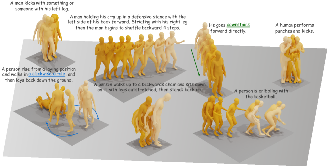
Figure 1: Our method can produce high-quality and diverse motion generation from a text prompt. The darker colours indicate later in the time pose.

2 Related Work

Non-diffusion methods. The seminal work Variational Auto-Encoders (VAE) [25] is utilized for human motion modelling. Motion Transformation VAE (MT-VAE) [51] break human motion into a series of atomic units [39], and use an LSTM encoder-decoder to reconstruct the motion. To account for noise [1] combines the root of variations with the previous pose. MotionCLIP [45] comprises a transformer-based motion auto-encoder. AvatarCLIP [22] utilize a volume rendering model to facilitate geometry sculpting and texture generation. TEMOS [34] utilize a transformer similar to ACTOR [33] to learn a joint motion and text space. Despite the decent result, the performance of VAE [25] based methods is restricted by the constraints imposed on the learned distributions.

Generative Adversarial Networks (GANs) [12] and Normalizing Flows (NFs) [37] on the other hand do not have the same constrain. HP-GAN [3], proposes a sequence-to-sequence model for probabilistic human motion prediction using a custom loss [2]. To account for motion blurriness [17] propose a robust transition technique based on adversarial recurrent networks. [48] breaks the generator into two components: a smooth-latent-transition component responsible for generating smooth latent frames and a global skeleton-decoder responsible for decoding each latent frame. Unlike GANs [12] or VAEs [25] Normalizing Flows (NFs) [37] can be trained efficiently using exact maximum likelihood. Inspired by GLOW [26], MoGlow [18] proposes an auto-regressive normalisation network to model motion sequences. Although GANs don’t impose constraints on target distribution they are hard to train and suffer from mode collapse [9, 28]. Normalizing flows on the other hand are limited in their expressiveness of complex distribution [27, 50].

Dffusion-based methods. Inspired by Nonequilibrium Thermodynamics, [43] propose a Markov chain of steps that slowly add noise to data samples (forward process) and learn to recover the noise with a neural network (revere process). After training, the learned reverse process resembles a generative model that can generate samples from random noise. With the great success of diffusion models [19, 38], research started to shift toward temporal data like videos [20, 4] and human motion [53, 5, 16]. MotionDiffuse [53] is one of the first works that applied diffusion to text-to-motion generation. They use transformer-based generator networks and work in the SMPL pose space [30]. MLD [5] learn a motion latent space with a transformer-based VAE and applied diffusion in the latent space. That allows them to train and sample with order of magnitude faster. However, this heavily depends on the latent space learned through the VAE, which is inherently lossy compression, especially with long sequences. We choose to follow a different approach to enhance sampling speed.

Despite their success, these approaches suffer from motion incoherence and are still limited to short temporal prediction [53, 5]. Besides that, previous work on temporal diffusion models [20, 4, 53, 5, 16] chose to treat the entire sequence as a single input without enforcing any temporal dependency. An exception is the work by [16], who use an autoregressive inverse process. Nonetheless, their forward process is kept the same and adds noise without any temporal dependency, which may lead to motion incoherence. Contrary to previous work, and inspired by recurrent networks [40, 24], we chose to design a new recurrent generative formulation. We propose a new diffusion model for generative temporal modelling RecMoDiffuse: Recurrent Flow Diffusion for Human Motion Generation. In RecMoDiffuse, both the forward and reverse processes respect temporal constraints as we add and recover the noise in an autoregressive manner, unlike previous formulations [53, 5, 52, 4, 49, 20]. This recurrent design allows us to skip diffusion steps during inference and reduces computation costs considerably.

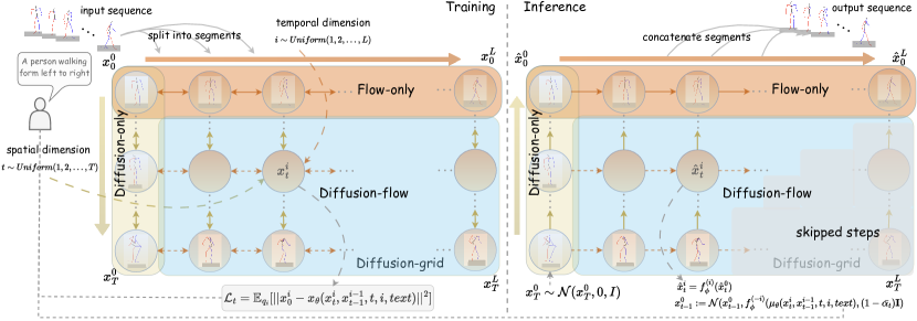
Figure 2: Method overview: RecMoDiffuse explicitly enforces temporal constant into the diffusion process, both forward and reverse processes follow temporal constraints. We propose alternate training (left): where we alternate between flow training on clean samples (flow-only) and diffusion with a fixed flow (diffusion-only and diffusion-flow). During inference (right), our design allows us to skip diffusion steps, which reduces computation costs during inference considerably compared to baselines.

3 Background

3.1 Diffusion Models

Diffusion models [43, 19] consist of two processes; a forward process that gradually adds noise to the data, and a reverse process recovers the noise, both follow a Markov chain. Recently, diffusion has been adapted for Text-to-Motion generation [53, 5], where diffusion is applied to pose space. Formally, given a data pair $(x^{(j)},u^{(j)})$, where $x^{(j)}$ represents the sequence of poses and $u^{(j)}$ is the language description of the motion sequence. Each sequence $x^{(j)}$ consists of $F$ frames $(\theta^{i\;(j)})\;i\in\{1,2,...,F\}$, where $\theta^{i\;(j)}\in\mathbb{R}^{D}$ represents pose state of $i$-th frame.

The generative distribution $p_{\theta}(x_{t-1}|x_{t})$ named the reverse process is defined as Gaussian transition and learned with a neural network :

$$p_{\theta}(x_{0:T}) :=p(x_{T})\prod_{t=1}^{T}p_{\theta}(x_{t-1}|x_{t})$$ (1)

$$p_{\theta}(x_{t-1}|x_{t}) :=\mathcal{N}(x_{t-1};\mu_{\theta}(x_{t},t,\varphi(u^{(j)})),\Sigma_{\theta}(x_{t},t,\varphi(u^{(j)}))).$$

Here $\mu_{\theta}(x_{t},t,\varphi(u^{(j)})),\Sigma_{\theta}(x_{t},t,\varphi(u^{(j)}))$ are parameterised by neural networks. $\varphi$ is a pre-trained neural network encoder that extracts embedding from the textual description $u^{(j)}$. The approximate posterior distribution $q(x_{t}|x_{t-1})$ of the diffusion model is called the forward process or the diffusion process. It follows a Markov chain and adds Gaussian noise gradually to the data according to a variance scheduler $\beta_{1},\beta_{2},...,\beta_{T}$, which can be learned [43] or fixed as a hyperparameter:

$$q(x_{1:T}|x_{0}) =\prod_{t=1}^{T}q(x_{t}|x_{t-1})$$ (2)

$$q(x_{t}|x_{t-1}) :=\mathcal{N}(x_{t};\sqrt{1-\beta_{t}}x_{t-1},\beta_{t}\mathbf{I}).$$

Training is performed by optimising the KL divergence between the forward and reverse processes. As suggested by [19] choosing a specific parametrization of $\mu_{\theta}(x_{t},t,\varphi(u^{(j)}))$, yield the loss $\mathcal{L}_{\theta}$:

$$\mathcal{L}_{\theta} =\mathbb{E}_{q}\left[w(t)\|x-f_{\theta}(x_{t},t,\varphi(u^{(j)}))\|^{2}\right]$$ (3)

Here $f_{\theta}(x_{t},t,\varphi(u^{(j)}))$ is a learnable neural network and the weight $w(t)$ can be freely specified. Efficient training can be achieved by using Monte Carlo integration to approximate the expectation. We uniformly sample time step $t$ and minimize the loss with stochastic gradient descent.

3.2 Normalizing Flows

A normalizing flow [37] is a transformation $Y=f(X)$ that transforms one random variable $X$ into a random variable $Y$ via successive transformations $f_{K}\circ f_{K-1}\circ...\circ f_{1}$, which are volume-preserving, invertible and bijective.

We utilize normalizing flows for human motion temporal modelling, specifically, given a data point $x^{(j)}$ consisting of $F$ frames sampled from a data distribution $q(\mathcal{X})$. We split each data point into $L$ segments $\{x^{i}\}_{i=0}^{L}$ , where each segment contains a predefined number of frames. Normalizing flow obtains the probability distribution of the next segment $x^{i+1}\sim P_{X^{i+1}}$ from a previous segment $x^{i}\sim P_{X^{i}}$. Using the change of variable theorem, we obtain

$$x^{i+1} =x_{K}=f_{K}\circ f_{K-1}\circ...\circ f_{1}(x^{i})$$ (4)

$$P_{X^{i+1}}(x^{i+1}) =P_{X^{i+1}}(x^{i})\prod_{k=1}^{K}\left|\det\left(\frac{\partial f_{k}(x_{k-1})}{\partial x_{k-1}}\right)\right|^{-1}.$$ (5)

Samples from the transformed distribution $P_{X^{i+1}}$ are generated by sampling from the base distribution $x^{i}\sim P_{X^{i}}$, then traverse the transformations in (4) to obtain a sample $x^{i+1}$.

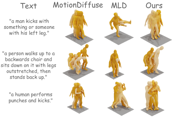
Figure 3: Qualitative comparison with the state-of-the-art methods on HumanML3D [13]. We provide the visualized motion results and real references from three text prompts. Our method generations match the textual descriptions.

4 Recurrent Flow Diffusion

Previous works in motion diffusion [53, 5, 16] model temporal data without enforcing any temporal relation in the diffusion process. Instead, the sequence is diffused as it is, treating each frame in the sampled sequence as temporally independent. We extend the diffusion model [43, 19] to the temporal dimension, by adding temporal connections between sequence frames, thereby enforcing temporal relations in the diffusion process.

The key idea is to create a recurrent diffusion structure similar to an RNN [40, 24, 21, 7]. In this way, both the forward and reverse processes will be temporally dependent. Each diffusion step in the forward process will depend ‘spatially’ on the previous diffused step on the same temporal step and ‘temporally’ on the previous segment diffused to the same step which creates what we refer to as diffusion grid as illustrated in Figure 2. We chose to model the temporal transition as a normalising flow model [37, 8, 26] as it preserves probability.

Next, we detail the forward and reverse processes and how the loss is obtained using a normalising flow to encode temporal dependency.

4.1 Forward process

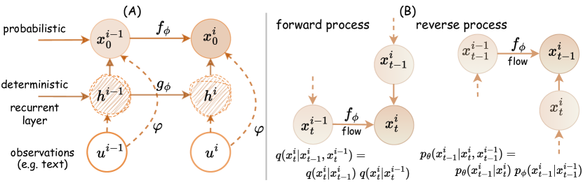
Figure 5: (A): Shows our LSTM [21] augmented normalizing flow transformation network (recurrent normalizing flow). (B): Shows forward and reverse processes of our diffusion model, both forward and reverse processes depend on the previous temporal and diffused steps.

Given a sequence and text data sample pair $(x^{(j)},u^{(j)})$, we split each sequence into L segments $\{x^{i}_{0}\}_{i=0}^{L}$ of equal length. We define the forward process in space and time by adding a small amount of noise following the diffusion grid to each data segment. In the case of the first segment $x^{0}_{0}$, we add Gaussian noise in the same way as in previous work , which we refer to as diffusion-only. For the other segments $\{x^{i}_{0},\;i>0\}$, unlike previous work [43, 19], we add noise following the diffusion grid, and we refer to it as the diffusion-flow see Figure 2. In the diffusion flow, we condition on the previous diffused step in the same temporal segment $x^{i}_{t-1}$ and on the previous segment diffused to the same step $x^{i-1}_{t}$. The forward process posterior can be factorised as follows; please refer to the Appendix Figure 5 (B):

$$q(x^{i}_{t}|x^{i}_{t-1},x^{i-1}_{t}) =q(x^{i}_{t}|x^{i}_{t-1})q(x^{i}_{t}|x^{i-1}_{t})$$ (6)

To get the noisy grid samples $x^{0:L}_{1},x^{0:L}_{2},...,x^{0:L}_{T}$ we add Gaussian noise in the diffusion-only and traverse the flow to the correct temporal step. As in [43, 19] the step size is controlled by the variance scheduler ${\beta_{t}\in(0,1)}_{t=0}^{T}$. The approximate posterior of the forward process $q(x^{1:L}_{1:T}|x^{0}_{0})$ is

$$q(x^{1:L}_{1:T}|x^{0}_{0}) =\prod_{i=1}^{L}\prod_{t=1}^{T}q(x^{i}_{t}|x^{i}_{t-1},x^{i-1}_{t}).$$ (7)

4.2 Reverse process

The generative process will follow the same grid but in reverse. Similar to the forward process of diffusion-only, we follow the same formulation as in [43, 19]. However, for the other segments $\{x^{i}_{0},\;i>0\}$, which lie in the diffusion-flow, we exploit temporal relations and condition the generative distribution on the previous reversed step on the same temporal segment $x^{i}_{t}$ and on the previous segment on the same diffused step $x^{i-1}_{t-1}$, as defined in the next equation; refer to Appendix B for more details.

$$p_{\theta}(x^{i}_{1:T}|x^{i}_{0},x^{i-1}_{T})=\prod_{t=1}^{T}p_{\theta}(x^{i}_{t-1}|x^{i}_{t},x^{i-1}_{t-1})$$ (8)

$$p_{\theta}(x^{0:L}_{0:T})=p(x^{0}_{T})\prod_{i=1}^{L}\prod_{t=1}^{T}p_{\theta}(x^{i}_{t-1}|x^{i}_{t},x^{i-1}_{t-1}).$$ (9)

For diffusion-only with very small noise variance $\beta_{t}$ the distribution of the reverse process follows a Gaussian distribution [10, 43], so that during learning only the mean and variance of the Gaussian need to be estimated. In the case of diffusion-flow we do not know the distribution of $q(x^{i}_{t}|x^{i}_{t-1},x^{i-1}_{t})$. Hence, the distribution of the reverse process $p_{\theta}(x^{i}_{t-1}|x^{i}_{t},x^{i-1}_{t-1})$ is also unknown. To address this problem, we can utilise the properties of normalising flows [37] and reverse the flow to the diffusion-only, where everything is Gaussian distributed. Sample from the Gaussian then traverse the flow transformations to the temporal step we need to get samples from as we can see in the next equation:

$$x^{0}_{t-1} :=\mathcal{N}(x^{0}_{t-1},f_{\phi}^{(-i)}(\mu_{\theta}(x^{i}_{t},x^{i-1}_{t-1},t,i,\varphi(u^{(j)})),(1-\bar{\alpha_{t}})\mathbf{I})$$ (10)

$$x^{i}_{t-1} =f_{\phi}^{(i)}(x^{0}_{t-1}),$$ (11)

where $\mu_{\theta}$ is a learnable neural network often called denoiser, both $(-i)$ and $(i)$ indicate traversing the inverse and forward flow $i$ times respectively, $f_{\phi}$ represent our flow model parameterized by $\phi$. $\varphi$ is a pre-trained CLIP model [36] that extracts embedding from the textual description $u^{i}$ as input.

4.3 Recurrent normalising flow

Inspired by [11], we augment the normalising flow [37, 8, 26] transformations with a deterministic recurrent network. This deterministic transformation records temporal information and acts like an auxiliary memory unit. We found it essential to have this augmented memory unit for the flow to learn temporal data; please refer to Appendix A for more details. The transition function of our recurrent normalising flow model is given by

$$h^{i} =g_{\phi_{h}}(h^{i-1},\varphi(u^{(j)}))$$ (12)

$$x^{i}_{0} =f_{\phi}(x^{i-1}_{0},h^{i},\varphi(u^{(j)})),$$

where $g_{\phi}$ and $f_{\phi}$ are LSTM cells and deep feed-forward networks, respectively. $\varphi$ is a pre-trained CLIP model [36].

We use a Real-NVP [8] as a probabilistic transformation and augment it with LSTM output features that act like a memory unit and we use the conditional coupling

$$=f_{\phi}(x^{i-1}_{0},h^{i},\varphi(u^{(j)}))$$ (13)

$$x^{i}_{0} =x^{i-1}_{0}\odot\sigma_{\phi}(x^{i-1}_{0},h^{i},\varphi(u^{(j)}))+\mu_{\phi}(x^{i-1}_{0},h^{i},\varphi(u^{(j)})),$$

where $\odot$ is element-wise multiplication and both $\sigma_{\phi}$ and $\mu_{\phi}$ are deep feed-forward networks.

We have now described the components of our model in the next subsection, we will discuss our loss and our training protocol.

Algorithm 1 Alternate training

1:Initialize update rate for flow (fHz) and diffusion (dHZ)

2:repeat

3:  unfreeze_flow_model($f{\phi}$)

4:  for every fHz do

5:      flow_update_step

6:  end for

7:  freeze_flow_model($f{\phi}$)

8:  for every dHz do

9:      diffusion_update_step

10:  end for

11:until convergence

Algorithm 2 diffusion_update_step

1:repeat

2:  $x_{0}\sim q(\mathcal{X})$ // sample sequence

3:  $x^{0}_{0}:=select\_at([x^{i}]_{i=0}^{L},0)$ // select 1st segment

4:  $t\sim Uniform({1,...,T})$

5:  $i\sim Uniform({0,...,L})$

6:  $\epsilon^{0}_{0}\sim\mathcal{N}(\mathbf{0},\mathbf{I})$

7:  $x^{i}_{t}=f^{(i)}_{\phi}(\sqrt{\bar{\alpha_{t}}}x^{0}_{0}+\sqrt{1-\bar{\alpha_{t}}}\epsilon^{0}_{t})$

8:  $x^{i-1}_{t}=f^{(i-1)}_{\phi}(\sqrt{\bar{\alpha_{t-1}}}x^{0}_{0}+\sqrt{1-\bar{\alpha_{t-1}}}\epsilon^{0}_{t-1})$

9:  Take gradient step on

10:      $\nabla_{\theta}\|x^{i}_{0}-f_{\theta}(x^{i}_{t},x^{i-1}_{t-1},t,i)\|^{2}$

11:until end of epoch

4.4 Training

Learning Recurrent Flow.

To learn the flow we assume every segment $x^{i}_{0}$ follows Dirac distribution and we minimize the KL divergence between the predictions and ground truth value. We also inflate the input to the flow with a Gaussian noise with a small standard deviation for more robustness as in [23]. See Appendix A for more details. Our KLs can be computed in a close form and the KLs are reduced to computing the MSE loss between the prediction and GT as in the next equation:

$$l_{single}=\|x^{i}_{0}-f_{\phi}(x^{i-1}_{0})\|^{2}$$ (14)

We found that learning with only the $l_{single}$ leads to prediction drift in multi-step prediction as the error accumulates. To learn a more robust multi-step prediction temporal model we use an additional loss $l_{multi}(\lambda)$ inspired by $TD(\lambda)$ learning [44]

$$l_{multi}(\lambda)=\sum_{i=0}^{L-1}\lambda^{i}\|x^{i+1}_{0}-f_{\phi}(\hat{x}^{i}_{0})\|^{2},$$ (15)

where $\hat{x}^{i}_{0}$ is the previously predicted segment. Our final flow loss becomes

$$\mathcal{L}_{flow}=l_{single}+w_{m}l_{multi}.$$ (16)

Learning Diffusion.

During training, we maximize the variational lower bound (VLB) of the log-likelihood of our diffusion grid which is simplified to (see Appendix E)

$$\mathcal{L}_{VLB} =\underbrace{D_{kl}(q(x^{0:L}_{T}|x^{0:L}_{0})\|p_{\theta}(x^{0:L}_{T}))}_{\mathcal{L}^{0:1}_{T}}+\sum_{t=2}^{T}\underbrace{D_{kl}(q(x^{0:L}_{t-1}|x^{0:L}_{t},x^{0:L}_{0})\|p_{\theta}(x^{0:L}_{t-1}|x^{0:L}_{t}))}_{\mathcal{L}^{0:L}_{t-1}}$$ (17)

$$\quad+\mathbb{E}_{q}[\underbrace{-\log(p_{\theta}(x^{0:L}_{0}|x^{0:L}_{1}))}_{\mathcal{L}^{0:L}_{0}}].$$

KL computation.

The intermediate KLs $\mathcal{L}^{1:L}_{t-1}$ follow unknown distributions which makes them problematic, as we use a non-linear flow; refer to Appendix E for more details. We utilize the normalising flow properties from Section 3.2, and use the reverse flow to take the predicted sample at frame $i$ to frame $0$ (diffusion-only). Hence, we can compute the KL in closed form as everything is Gaussian distributed, and then we transfer back to temporal step $i$ following the forward flow.

In the diffusion-only we follow similar choices to [19] and choose to learn only the mean of the distribution and set the variance to a fixed value $\sigma_{t}=\beta_{t}$. We arrive at a similar formula as in [19] with additional weighting terms based on the normalising flow transformation $|\det\frac{\partial f}{\partial x^{i}_{0}}|^{-1}$ :

$$\mathcal{L}_{t-1}^{i}=\mathbb{E}_{q}\left[w(t)\left|\det\frac{\partial f_{\phi}}{\partial x^{i}_{0}}\right|^{-1}\|x^{i}_{0}-f_{\theta}(x^{i}_{t},f^{i-1}_{t-1},t,i)\|^{2}\right].$$ (18)

Here, $x^{i}_{0}$ is the clean segment at temporal step $i$ and $f_{\theta}$ is a learnable neural network that predicts a clean segment; refer to Appendix E for a full derivation. We compute this expectation by means of Monte Carlo integration and we uniformly sample random spacial step $t$ and temporal step $i$ and traverse the flow to get to the temporal location see Figure 2.

Training protocol.

We found our flow can easily overfit, leading the denoiser model to have unstable training. Therefore we alternate between flow and diffusion training with different update rates. We train the flow on clean segments only (flow-only) and when updating the denoiser we freeze the flow and learn to denoise corrupted segments following the diffusion-grid as in Algorithm 1.

Sampling.

Unlike previous methods [53, 5, 16], we do not need to denoise samples with full sequence size. Instead, utilizing the flow model we can skip diffusion steps by sampling in a staircase through the diffusion grid see Figure  2 (B). This makes our model computationally efficient in dealing with temporal data and has higher throughput compared to baselines, see Appendix B and C.

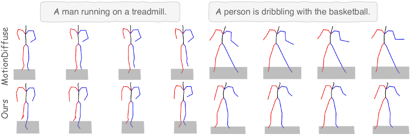
Figure 4: Qualitative results on the HumanML3D dataset. We compare our method with MotionDiffuse [53] and visualize two examples for each given prompt. Our method achieves comparable results with MotionDiffuse.

Method	R-Precision ($\uparrow$)			FID ($\downarrow$)	MultiModal Dist ($\downarrow$)	Diversity ($\rightarrow$)	MultiModality
	Top 1	Top 2	Top 3
Real motions	$0.511^{\pm.003}$	$0.703^{\pm.002}$	$0.797^{\pm.003}$	$0.002^{\pm.000}$	$2.974^{\pm.008}$	$9.503^{\pm.065}$	-
TEMOS	$0.424^{\pm.002}$	$0.612^{\pm.002}$	$0.722^{\pm.002}$	$3.734^{\pm.028}$	$3.703^{\pm.008}$	$8.973^{\pm.071}$	$0.368^{\pm.018}$
T2M	$0.457^{\pm.002}$	$0.639^{\pm.003}$	$0.740^{\pm.003}$	$1.067^{\pm.002}$	$3.340^{\pm.008}$	$9.188^{\pm.002}$	$2.090^{\pm.083}$
MDM	$0.320^{\pm.005}$	$0.498^{\pm.004}$	$0.611^{\pm.007}$	$0.544^{\pm.044}$	$5.566^{\pm.027}$	$9.559^{\pm.086}$	$2.799^{\pm.072}$
MotionDiffuse	$0.491^{\pm.001}$	$0.681^{\pm.001}$	$0.782^{\pm.001}$	$0.630^{\pm.001}$	$3.113^{\pm.001}$	$9.410^{\pm.049}$	$1.553^{\pm.042}$
MLD	$0.481^{\pm.003}$	$0.673^{\pm.003}$	$0.772^{\pm.002}$	$0.473^{\pm.013}$	$3.196^{\pm.010}$	$9.724^{\pm.082}$	$2.413^{\pm.079}$
AMD	$-$	$-$	$0.617^{\pm.014}$	$0.586^{\pm.107}$	$5.469^{\pm.063}$	$9.769^{\pm.096}$	$2.512^{\pm.232}$
Ours-4 segments	$0.4116^{\pm.0063}$	$0.5941^{\pm.0039}$	$0.7023^{\pm.0042}$	$0.4122^{\pm.0161}$	$3.6038^{\pm.0061}$	$8.2115^{\pm.0159}$	$1.5437^{\pm.0459}$

Table 1: Quantitative results on the HumanML3D [13] test set. All methods use the real motion length from the ground truth. We ran all the evaluations 20 times and reported a $95\%$ CI.

Method	R-Precision ($\uparrow$)			FID ($\downarrow$)	MultiModal Dist ($\downarrow$)	Diversity ($\rightarrow$)	MultiModality
	Top 1	Top 2	Top 3
Real motions	$0.5138$	$0.6957$	$0.7937$	$0.002^{\pm.000}$	$2.974^{\pm.008}$	$9.5046^{\pm.065}$	-
TEMOS	$0.353^{\pm.006}$	$0.561^{\pm.007}$	$0.687^{\pm.005}$	$3.717^{\pm.051}$	$3.417^{\pm.019}$	$10.84^{\pm.100}$	$0.532^{\pm.034}$
T2M	$0.370^{\pm.005}$	$0.569^{\pm.007}$	$0.693^{\pm.007}$	$2.770^{\pm.109}$	$3.401^{\pm.008}$	$10.91^{\pm.119}$	$1.482^{\pm.065}$
MDM	$0.164^{\pm.004}$	$0.291^{\pm.004}$	$0.396^{\pm.004}$	$0.497^{\pm.021}$	$9.191^{\pm.022}$	$10.85^{\pm.109}$	$1.907^{\pm.214}$
MotionDiffuse	$0.417^{\pm.004}$	$0.621^{\pm.004}$	$0.739^{\pm.004}$	$1.954^{\pm.062}$	$2.958^{\pm.005}$	$11.10^{\pm.143}$	$0.730^{\pm.013}$
MLD	$0.390^{\pm.008}$	$0.609^{\pm.008}$	$0.734^{\pm.007}$	$0.404^{\pm.027}$	$3.204^{\pm.027}$	$10.80^{\pm.117}$	$2.192^{\pm.071}$
Ours-4 segments	$0.3644^{\pm.0077}$	$0.5763^{\pm.0077}$	$0.7121^{\pm.0061}$	$1.95^{\pm.0512}$	$3.5409^{\pm.0203}$	$10.0622^{\pm.1120}$	$1.0676^{\pm.0453}$

Table 2: Quantitative results on the KIT-ML [35] test set. All methods use the real motion length from the ground truth. We ran all the evaluations 20 times and reported a $95\%$ CI.

Method	Total Inference Time (mins)	FLOPs (G)	Parameters
MotionDiffuse	$3.495^{\pm.052}$	$9.97$	$x\in\mathbb{R}^{196\times 251}$
Ours-4 segments	$1.118^{\pm.127}$	$2.98$	$x\in\mathbb{R}^{49\times 251}$
Ours-7 segments	$0.994^{\pm.011}$	$2.27$	$x\in\mathbb{R}^{28\times 251}$
Ours-14 segments	$5.259^{\pm 3.579}$	$4.03$	$x\in\mathbb{R}^{14\times 251}$

Table 3: Inference time comparison. Our method can skip diffusion steps, which leads to lower inference time compared to state-of-the-art methods that need to diffuse through the full sequence.

5 Experiments

Datasets.

KIT Motion Language dataset  [35] provides 3911 motion sequences and 6353 sequence-level natural language descriptions. HumanML3D  [13] re-annotates the AMASS dataset  [31] and the HumanAct12 dataset  [15]. It provides 44970 annotations on 14616 motion sequences.

Evaluation Metrics.

We follow the same evaluation protocol as [53, 5] and evaluate all methods with five different metrics and report Frechet Inception Distance (FID), R Precision, Diversity, Multimodality and Multi-modal Distance. We run each evaluation 20 times and report the statistic interval with $95$ confidence.

Qualitative evaluation.

Figure 3 and 4 show our methods can produce plausible motion sequences and reflect the text input caption on par with the diffusion-based baselines MotionDiffuse [53] and MLD [5]. Smoothness and motion coherence are not reflected well in the static figures we refer the reader to see our generated videos.

Quantitative evaluation.

We compare our model against diffusion-based state-of-the-art baselines MotionDiffuse [53], MLD [5] AMD [16], and other non-diffusion-base methods TEMOS [34] and T2M [14]. Table 1 and Table 2 show our method archives a comparable result with the state-of-the-art methods on the KIT-ML and the HumnamL3D datasets respectively.

Inference time.

Although our methods achieve comparable results to state-of-the-art methods we are considerably faster at inference time, and our framework allows us to skip diffusion steps. We can control the throughput of our model by carefully designing our model using the number of segments and following different sampling paths. Table 3 shows the speed gain following our diffusion-grid staircase sampling. We ran all the evaluations on a $128$ batch size with $196$ sequence lengths $20$ times on a single NVIDIA V100 GPU and reported mean inference time and standard deviation. Please refer to Appendix C for further ablations and D for implementation details.

6 Limitations

Although our method generates coherence motion sequences, it suffers from notable limitations. It requires training normalizing flow first to have a stable diffusion loss, which can be numerically unstable. This numerical instability is problematic, especially when the number of segments becomes large. Like other diffusion models, it requires large diffusion steps.

7 Conclusion

We present RecMoDiffuse, the first model to bring diffusion into the temporal dimension, by formulating a recurrent diffusion model for generative temporal modelling. Our recurrent formulation explicitly enforces temporal constraints in the diffusing process. It adds and recovers noise in an autoregressive manner. We demonstrated the effectiveness of our method in human motion generation, both quantitative and qualitative results showed that our method performs on par with the state-of-the-art generative models while enjoying lower computational complexity during inference.

We believe RecMoDiffuse is one step forward in better designing temporal diffusion models and better utilizing their power for temporal modelling. Finally, our approach naturally extends to latent space, and we can enjoy more computational efficiency during training and inference, but we leave those avenues for future exploration.

Appendix

Appendix A Recurrent Normalizing Flow

Inspired by [11], we augment the normalising flow [37, 8, 26] transformations with a deterministic recurrent network. This deterministic transformation records temporal information and acts like an auxiliary memory unit. We found it essential to have this augmented memory unit for the flow to learn temporal data. The transition function of our recurrent normalising flow model is given by:

$$h^{i} =g_{\phi_{h}}(h^{i-1},\varphi(u^{(j)}))$$ (19)

$$x^{i}_{0} =f_{\phi}(x^{i-1}_{0},h^{i},\varphi(u^{(j)}))$$

where $g_{\phi}$ and $f_{\phi}$ are LSTM cells and deep feed-forward networks, respectively. $\varphi$ is a pre-trained CLIP model [36].

We use a Real-NVP [8] as a probabilistic transformation and augment it with LSTM output features that act like a memory unit and we use the following conditional coupling:

$$=f_{\phi}(x^{i-1}_{0},h^{i},\varphi(u^{(j)}))$$ (20)

$$x^{i}_{0} =x^{i-1}_{0}\odot\sigma_{\phi}(x^{i-1}_{0},h^{i},\varphi(u^{(j)}))+\mu_{\phi}(x^{i-1}_{0},h^{i},\varphi(u^{(j)}))$$

where $\odot$ is element-wise multiplication and both $\sigma_{\phi}$ and $\mu_{\phi}$ are deep feed-forward networks.

During training, we inflate the input to the flow with a Gaussian noise with a small standard deviation for more robustness as in [23].

$$\tilde{x}^{i-1}_{0} =x^{i-1}_{0}+\epsilon_{i}\text{ where }\epsilon_{i}\sim\mathcal{N}(0,\sigma_{inf}I)$$ (21)

$$[\sigma_{\phi},\mu_{\phi}] =f_{\phi}(\tilde{x}^{i-1}_{0},h^{i},\varphi(u^{(j)}))$$

$$x^{i}_{0} =x^{i-1}_{0}\odot\sigma_{\phi}(\tilde{x}^{i-1}_{0},h^{i},\varphi(u^{(j)}))+\mu_{\phi}(\tilde{x}^{i-1}_{0},h^{i},\varphi(u^{(j)}))$$

A.1 Numerical instability

Normalizing flow is not designed for temporal modelling, although we tried to remedy that and augment it with an LSTM and added the multi-step loss 15. When computing the inverse flow with multi-step prediction, they still suffer from numerical instability. The main source of this is the $\sigma_{\phi}$ function in the mapping. If the values are really large this will cause an overflow of the inverse mapping $f^{(-i)}_{\phi}$ and result in a NaN in the loss. We tried to clamp the values to an acceptable range and applied a HardTanh function with a min and max limit of $-0.1\text{ and }0.1$ respectively. This solves the instability issue with the loss, but we still can not do a very long recurrence. We believe this is a limitation of the current method and it needs further explanation which we leave for future work.

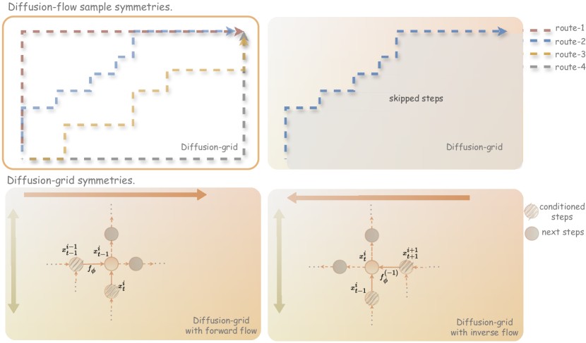
Figure 6: Diffusion-flow symmetries. By design, we can arrive at diffusion-flow samples following different routes. Some routes are more efficient than others as they allow for skipping diffusion sampling steps, but all are mathematically equivalent. Diffusion-grid symmetries. Normalizing flow properties gives us two grids (forward-flow and inverse-flow). Both are mathematically equivalent, but the forward-flow is more numerically stable.

Appendix B Notes on our recurrent formulation properties

The design of our grid-diffusion gives some natural symmetries, which allow for skipping diffusion sampling steps. That leads to more efficient inference. With the proper design, we can utilize that for efficient training but with less flexibility during inference. In this section, we will talk in detail about those properties.

Diffusion-flow sample symmetries.

By design we can arrive at diffusion-flow samples following different routes, some are more efficient than others but are all mathematically equivalent, see Figure 6. Empirically on the other hand some produce better sample quality, more specifically when using the flow to get temporal samples we have lower quality. The reason is the normalizing flow is the less capacity network and not well-suited for temporal modelling. As for computational efficiency, some routes are more efficient than others. Because the denoising process is more expensive with larger sequence lengths, routes that allow us fewer diffusion steps result in more computationally efficient inference. This design allows us to trade-off between computational efficiency and sample quality. See Figure 6 for different route comparisons.

Diffusion-grid symmetries.

As normalizing flow is an invertible transformation we can have two grids one with forward flow and one with inverse flow. Using that we can condition the reverse process using $x^{i+1}_{t-1}$ or $x^{i-1}_{t-1}$, both are mathematically equivalent but the latter is more numerically stable as we don’t need to compute additional flow inverse transformation. What we used to parameterize the reverse flow and the loss as we described in the next section.

Appendix C RecMoDiffuse sampling

As mentioned in the main text, unlike previous methods [53, 5, 16], we do not need to sample Gaussian noise with full sequence size. Instead, utilizing the flow model we can skip diffusion steps by sampling in a staircase through the diffusion grid. This makes our model computationally efficient in dealing with temporal data and has higher throughput.

When to start sampling in a staircase gives us the unique ability to trade off between computation complexity and sampling quality. The two extremes are generating the first segment with diffusion-only and then rolling out with the normalizing flow with flow-only giving the lowest quality and the lowest computational complexity. We refer to as disentangle as we disentangle the diffusion space and time during sampling. The second is to start the staircase from the beginning with diffusion-flow which gives the highest computation complexity and better sampling quality depending on when to start the staircase sampling. See Table  5 and Table  6.

Algorithm 3 Sampling

1:$x^{0}_{T}\sim\mathcal{N}(0,I)$

2:$\mathcal{S}_{out}:=[x^{0}_{T},f_{\phi}(x^{0}_{T})]$

3:for $t=T,...,1$ do

4:  $\mathcal{S}=\mathcal{S}_{out}$

5:  for $j=0,...,i+1$ do

6:   $z\sim\mathcal{N}(0,I)$ if $t>1$ else $z=\mathbf{0}$

7:   $x^{j}_{t}=S[j]$

8:   $x^{j-1}_{t-1}=S_{out}[j-1]$ if $j>0$ else $x^{j-1}_{t-1}=\mathbf{0}$

9:   $x^{0}_{t}=f^{(-j)}_{\phi}(S[j])$

10:   $\epsilon^{0}_{\theta}=f^{(-j)}_{\phi}(\epsilon_{\theta}(x^{j}_{t},x^{j-1}_{t-1},t,j))$

11:   $x^{0}_{t-1}=\frac{1}{\sqrt{\alpha_{t}}}(x^{0}_{t}-\frac{1-\alpha_{t}}{\sqrt{1-\bar{\alpha_{t}}}}\epsilon^{0}_{\theta})+\sigma_{t}z$

12:   $x^{j}_{t-1}=f^{(j)}_{\phi}(x^{0}_{t-1})$

13:   $\mathcal{S}_{out}.append(x^{j}_{t-1})$

14:  end for

15:  return $\mathcal{S}_{out}$

16:end for

17:return $\mathcal{S}_{out}$

Method	R-Precision ($\uparrow$)			FID ($\downarrow$)	MultiModal Dist ($\downarrow$)	Diversity ($\rightarrow$)	MultiModality
	Top 1	Top 2	Top 3
Real motions	$0.5138$	$0.6957$	$0.7937$	$0.002^{\pm.000}$	$2.974^{\pm.008}$	$9.5046^{\pm.065}$	-
Ours-4 segments	$0.3624^{\pm.0068}$	$0.5639^{\pm.0069}$	$0.6879^{\pm.0062}$	$0.0^{\pm.001}$	$3.6536^{\pm.0204}$	$9.8560^{\pm.0965}$	$1.1339^{\pm.0384}$
Ours-7 segments	$0.3221^{\pm.01}$	$0.5199^{\pm.0153}$	$0.6449^{\pm.0107}$	$4.9101^{\pm.2297}$	$4.151^{\pm.0456}$	$8.8144^{\pm.2913}$	$1.2737^{\pm.1011}$

Table 4: Quantitative results on the KIT-ML [35] test set. All methods use the real motion length from the ground truth. We ran all the evaluations 20 times and reported a $95\%$ confidence interval.

Method	R-Precision ($\uparrow$)			FID ($\downarrow$)	MultiModal Dist ($\downarrow$)	Diversity ($\rightarrow$)	MultiModality
	Top 1	Top 2	Top 3
Real motions	$0.5138$	$0.6957$	$0.7937$	$0.002^{\pm.000}$	$2.974^{\pm.008}$	$9.5046^{\pm.065}$	-
Entangle-997	$0.3624^{\pm.0068}$	$0.5639^{\pm.0069}$	$0.6879^{\pm.0062}$	$4.7260^{\pm.1823}$	$3.6536^{\pm.0204}$	$9.8560^{\pm.0965}$	$1.1339^{\pm.0384}$
Entangle-980	$0.3022^{\pm.0091}$	$0.4954^{\pm.0084}$	$0.6161^{\pm.0063}$	$6.2045^{\pm.1114}$	$4.4230^{\pm.05}$	$9.0687^{\pm.1126}$	$1.6361^{\pm.1407}$
Entangle-900	$0.2901^{\pm.0071}$	$0.4670^{\pm.0071}$	$0.5884^{\pm.0067}$	$8.1093^{\pm.3235}$	$4.7800^{\pm.0533}$	$8.5817^{\pm.1952}$	$1.6708^{\pm.0817}$

Table 5: Quantitative results on the KIT-ML [35] test set. All methods use the real motion length from the ground truth. We ran all the evaluations 20 times and reported a $95\%$ confidence interval.

Method (Ours-4s)	Total Inference Time (mins)	FLOPs (G)	Parameters
Disentangle	$1.522^{\pm.038}$	$1.38$	$x\in\mathbb{R}^{49\times 251}$
Entangle-997	$1.118^{\pm.127}$	$2.98$	$x\in\mathbb{R}^{49\times 251}$
Entangle-980	$1.418^{\pm.028}$	$3.23$	$x\in\mathbb{R}^{49\times 251}$
Entangle-900	$1.966^{\pm.047}$	$4.41$	$x\in\mathbb{R}^{49\times 251}$

Table 6: Inference time comparison. RecMoDiffuse can skip diffusion steps, which leads to lower inference time compared to state-of-the-art methods that need to diffuse through the full sequence.

Appendix D Implementation details

Training settings.

We train our model using MoMo-Adam optimizer  [42] with a learned rate $1e^{-4}$ for the flow and $2e^{-4}$ learning rate for the diffusion denoiser model, with a batch size $128$. Our full training takes $10$ days on 4 V-100 Nvidia GPUs and $5$ days on 2 A-100 Nvidia GPUs. We train the full model for $50$ epochs in total and we artificially increased the data length by a factor of $25$ for each GPU used. For our alternate training, the rate for diffusion denoiser update to flow update is 5 to 1, i.e. for every 5 epochs updates to the diffusion denoiser we update the flow model once until we reach epoch 25 then we only update the diffusion denoiser. We trained the flow with $w_{m}=1$ and $\lambda=0.99$ in all experiments.

For Inferenace time comparison and computational efficiency we ran all the evaluations on a $128$ batch size with $196$ sequence lengths $20$ times and reported mean inference time and standard deviation. For the FLOPs, we use calflops python package to calculate the flops on a batch size of $1$ with $196$ sequence length. We ran both experiments on a single NVIDIA V100 GPU.

Architectures.

We use $4$ segments for a maximum sequence length of $196$, which sets the segment length to $49$ frames. For normalizing flow, we used 2 layers LSTM with $512$ hidden dimensions, and for the invertible transformation, we used $128$ feature dimensions 3 transformation blocks, and $0.5$ layer and input dropout rate. For diffusion denoiser we utilize a similar temporal transformer-based architecture as in  [53]. We used 8 transfer layers with $512$ latent dimensions and with $8$ heads. As for the text conditioning, we used a pre-trained CLIP ViT-B/32 model  [36] to encode text and then added four more transformer encoder layers. The latent dimension of the text encoder and the motion decoder are $256$ and $512$, respectively. As for the diffusion model, the number of diffusion steps is $1000$, and the variances $\beta_{t}$ are linearly from $0.0001$ to $0.02$.

To add temporal conditioning we used positional encoding with different frequencies to the diffusion frame number, and we used different shallow MLPs to encode the temporal and spacial step to latent spaces. We follow the same conditioning method as in  [53] and add the mapped latents of fame and time to the projected text embedding and apply cross-attention with the transformer to predict the denoiser similar to  [53].

Appendix E Loss derivation (proof)

We use diffusion-grid with forward flow defined in the previous section B. As discussed in the main text our forward process of the diffusion grid is defined by the next equations:

$$q(x^{i}_{1:T}|x^{i}_{0},x^{i-1}_{T}) =\prod_{t=1}^{T}q(x^{i}_{t}|x^{i}_{t-1},x^{i-1}_{t})$$ (22)

$$q(x^{1:L}_{1:T}|x^{0}_{0},x^{0-1}_{T}) =\prod_{t=1}^{T}q(x^{1:L}_{t}|x^{1:L}_{t-1})$$ (23)

$$q(x^{1:L}_{1:T}|x^{0}_{0},x^{0-1}_{T}) =\prod_{i=1}^{L}\prod_{t=1}^{T}q(x^{i}_{t}|x^{i}_{t-1},x^{i-1}_{t})$$ (24)

As we are using diffusion-grid with forward flow then, our reverse process is defined by the next equations:

$$p_{\theta}(x^{i}_{1:T}|x^{i}_{0},x^{i-1}_{T})=\prod_{t=1}^{T}p_{\theta}(x^{i}_{t-1}|x^{i}_{t},x^{i-1}_{t-1})$$ (25)

$$p_{\theta}(x^{0:L}_{0:T})=p(x^{0:L}_{T})\prod_{t=1}^{T}p_{\theta}(x^{0:L}_{t-1}|x^{0:L}_{t})$$ (26)

$$p_{\theta}(x^{0:L}_{0:T})=p(x^{0}_{T})\prod_{i=1}^{L}\prod_{t=1}^{T}p_{\theta}(x^{i}_{t-1}|x^{i}_{t},x^{i-1}_{t-1})$$ (27)

Let us begin by equating our data log probability $\log(p_{\theta}(x^{0:L}_{0}))$ as follows:

$$-\log(p_{\theta}(x^{0:L}_{0})) \leq-\log(p_{\theta}(x^{0:L}_{0}))+D_{kl}(q(x^{0:L}_{1:T}|x^{0:L}_{0})\|p_{\theta}(x^{0:L}_{1:T}|x^{0:L}_{0}))$$

$$=-\log(p_{\theta}(x^{0:L}_{0}))+\mathbb{E}_{x^{0:L}_{1:T}\sim q(x^{0:L}_{1:T}|x^{0:L}_{0})}\big{[}\log\frac{q(x^{0:L}_{1:T}|x^{0:L}_{0})}{p_{\theta}(x^{0:L}_{0:T})/p_{\theta}(x^{0:L}_{0})}\big{]}$$

$$=\mathbb{E}_{q}\big{[}\log\frac{q(x^{0:L}_{1:T}|x^{0:L}_{0})}{p_{\theta}(x^{0:L}_{0:T})}\big{]}$$

Then let $\mathcal{L}_{VLB}=\mathbb{E}_{q(x^{0:L}_{0:T})}\big{[}\log\frac{q(x^{0:L}_{1:T}|x^{0:L}_{0})}{p_{\theta}(x^{0:L}_{0:T})}\big{]}\geq-\mathbb{E}_{q(x^{0:L}_{0:T})}p_{\theta}(x^{0:L}_{0})$

$$\mathcal{L}_{VLB} =\mathbb{E}_{q}\big{[}\log\frac{q(x^{0:L}_{1:T}|x^{0:L}_{0})}{p_{\theta}(x^{0:L}_{0:T})}\big{]}$$

$$=\mathbb{E}_{q}\big{[}\log\frac{\prod_{t=1}^{T}q(x^{0:L}_{t}|x^{0:L}_{t-1})}{p_{\theta}(x^{0:L}_{T})\prod_{t=1}^{T}p_{\theta}(x^{0:L}_{t-1}|x^{0:L}_{t})}\big{]}$$

$$=\mathbb{E}_{q}\big{[}-\log(p_{\theta}(x^{0:L}_{T}))+\sum_{t=1}^{T}\log\frac{q(x^{0:L}_{t}|x^{0:L}_{t-1})}{p_{\theta}(x^{0:L}_{t-1}|x^{0:L}_{t})}\big{]}$$

$$=\mathbb{E}_{q}\big{[}-\log(p_{\theta}(x^{0:L}_{T}))+\sum_{t=2}^{T}\log\frac{q(x^{0:L}_{t}|x^{0:L}_{t-1})}{p_{\theta}(x^{0:L}_{t-1}|x^{0:L}_{t})}+\log\frac{q(x^{0:L}_{1}|x^{0:L}_{0})}{p_{\theta}(x^{0:L}_{0}|x^{0:L}_{1})}\big{]}$$

$$=\mathbb{E}_{q}\big{[}-\log(p_{\theta}(x^{0:L}_{T}))+\sum_{t=2}^{T}\log\big{(}\frac{q(x^{0:L}_{t-1}|x^{0:L}_{t},x^{0:L}_{0})}{p_{\theta}(x^{0:L}_{t-1}|x^{0:L}_{t})}.\frac{q(x^{0:L}_{t}|x^{0:L}_{0})}{q(x^{0:L}_{t-1}|x^{0:L}_{0})}\big{)}+\log\frac{q(x^{0:L}_{1}|x^{0:L}_{0})}{p_{\theta}(x^{0:L}_{0}|x^{0:L}_{1})}\big{]}\;\;\text{(Bayes's rule)}$$

$$=\mathbb{E}_{q}\big{[}-\log(p_{\theta}(x^{0:L}_{T}))+\sum_{t=2}^{T}\log\frac{q(x^{0:L}_{t-1}|x^{0:L}_{t},x^{0:L}_{0})}{p_{\theta}(x^{0:L}_{t-1}|x^{0:L}_{t})}+\sum_{t=2}^{T}\log\frac{q(x^{0:L}_{t}|x^{0:L}_{0})}{q(x^{0:L}_{t-1}|x^{0:L}_{0})}+\log\frac{q(x^{0:L}_{1}|x^{0:L}_{0})}{p_{\theta}(x^{0:L}_{0}|x^{0:L}_{1})}\big{]}$$

$$=\mathbb{E}_{q}\big{[}-\log(p_{\theta}(x^{0:L}_{T}))+\sum_{t=2}^{T}\log\frac{q(x^{0:L}_{t-1}|x^{0:L}_{t},x^{0:L}_{0})}{p_{\theta}(x^{0:L}_{t-1}|x^{0:L}_{t})}+\log\frac{q(x^{0:L}_{T}|x^{0:L}_{0})}{q(x^{0:L}_{1}|x^{0:L}_{0})}+\log\frac{q(x^{0:L}_{1}|x^{0:L}_{0})}{p_{\theta}(x^{0:L}_{0}|x^{0:L}_{1})}\big{]}$$

(Intermediate terms cancels)

$$=\mathbb{E}_{q}\big{[}\log\frac{q(x^{0:L}_{T}|x^{0:L}_{0})}{p_{\theta}(x^{0:L}_{T})}+\sum_{t=2}^{T}\log\frac{q(x^{0:L}_{t-1}|x^{0:L}_{t},x^{0:L}_{0})}{p_{\theta}(x^{0:L}_{t-1}|x^{0:L}_{t})}-\log(p_{\theta}(x^{0:L}_{0}|x^{0:L}_{1}))\big{]}\;\;\text{(Rearranging logs)}$$

$$=\mathbb{E}_{q}\big{[}\underbrace{D_{kl}(q(x^{0:L}_{T}|x^{0:L}_{0})\|p_{\theta}(x^{0:L}_{T}))}_{\mathcal{L}^{0:1}_{T}}+\sum_{t=2}^{T}\underbrace{D_{kl}(q(x^{0:L}_{t-1}|x^{0:L}_{t},x^{0:L}_{0})\|p_{\theta}(x^{0:L}_{t-1}|x^{0:L}_{t}))}_{\mathcal{L}^{0:L}_{t-1}}+\mathbb{E}_{q}[\underbrace{-\log(p_{\theta}(x^{0:L}_{0}|x^{0:L}_{1}))}_{\mathcal{L}^{0:L}_{0}}]\big{]}$$

Let us label each term in the lower bound separately and further expand them:

$$\mathcal{L}^{0:1}_{T} =D_{kl}(q(x^{0:L}_{T}|x^{0:L}_{0})\|p_{\theta}(x^{0:L}_{T}))=\mathbb{E}_{q}[\log\big{(}\frac{q(x^{0}_{T}|x^{0}_{0})\prod_{i=1}^{L}q(x^{i}_{T}|x^{i}_{0},x^{i-1}_{T})}{p_{\theta}(x^{0}_{T})\prod_{i=1}^{L}p_{\theta}(x^{i}_{T}|x^{i-1}_{T})}\big{)}]$$

$$=\mathbb{E}_{q}\big{[}\log\frac{q(x^{0}_{T}|x^{0}_{0})}{p_{\theta}(x^{0}_{T})}+\sum_{i=1}^{L}\log\frac{q(x^{i}_{T}|x^{i}_{0},x^{i-1}_{T})}{p_{\theta}(x^{i}_{T}|x^{i-1}_{T})}\big{]}$$

$$=\underbrace{D_{kl}(q(x^{0}_{T}|x^{0}_{0})\|p_{\theta}(x^{0}_{T}))}_{L^{0}_{T}}+\sum_{i=1}^{L}\underbrace{D_{kl}(q(x^{i}_{T}|x^{i}_{0},x^{i-1}_{T})\|p_{\theta}(x^{i}_{T}|x^{i-1}_{T}))}_{L^{i}_{T}}$$

$$\mathcal{L}^{0:L}_{0} =-\log(p_{\theta}(x^{0:L}_{0}|x^{0:L}_{1}))=-\log(p_{\theta}(x^{0}_{0}|x^{0}_{1})-\log(\prod_{i=1}^{L}p_{\theta}(x^{i}_{0}|x^{i-1}_{0},x^{i}_{1})))$$

$$=\underbrace{-\log(p_{\theta}(x^{0}_{0}|x^{0}_{1})}_{\mathcal{L}^{0}_{0}}+\sum_{i=1}^{L}\underbrace{-\log(p_{\theta}(x^{i}_{0}|x^{i-1}_{0},x^{i}_{1})))}_{\mathcal{L}^{i}_{0}}$$

$$\mathcal{L}^{0:L}_{t-1} =D_{kl}(q(x^{0:L}_{t-1}|x^{0:L}_{t},x^{0:L}_{0})\|p_{\theta}(x^{0:L}_{t-1}|x^{0:L}_{t}))=\log\frac{q(x^{0:L}_{t-1}|x^{0:L}_{t},x^{0:L}_{0})}{p_{\theta}(x^{0:L}_{t-1}|x^{0:L}_{t})}$$

$$=\log\big{(}\frac{q(x^{0}_{t-1}|x^{0}_{t},x^{0}_{0})\prod_{i=1}^{L}q(x^{i}_{t-1}|x^{i}_{t},x^{i-1}_{t-1},x^{i}_{0})}{p_{\theta}(x^{0}_{t-1}|x^{0}_{t})\prod_{i=1}^{L}p_{\theta}(x^{i}_{t-1}|x^{i}_{t},x^{i-1}_{t-1})}\big{)}=\mathbb{E}_{q}[\log\frac{q(x^{0}_{t-1}|x^{0}_{t},x^{0}_{0})}{p_{\theta}(x^{0}_{t-1}|x^{0}_{t})}+\sum_{i=1}^{L}\log\frac{q(x^{i}_{t-1}|x^{i}_{t},x^{i-1}_{t-1},x^{i}_{0})}{p_{\theta}(x^{i}_{t-1}|x^{i}_{t},x^{i-1}_{t-1})}]$$

$$=\underbrace{D_{kl}(q(x^{0}_{t-1}|x^{0}_{t},x^{0}_{0})\|p_{\theta}(x^{0}_{t-1}|x^{0}_{t}))}_{\mathcal{L}^{0}_{t-1}}+\sum_{i=1}^{L}\underbrace{D_{kl}(q(x^{i}_{t-1}|x^{i}_{t},x^{i-1}_{t-1},x^{i}_{0})\|p_{\theta}(x^{i}_{t-1}|x^{i}_{t},x^{i-1}_{t-1}))}_{\mathcal{L}^{i}_{t-1}}$$

Our final variational lower bound $\mathcal{L}_{VLB}$ takes the forum:

$$\mathcal{L}_{VLB} =\sum_{i=0}^{L}\sum_{t=0}^{T}\mathcal{L}^{i}_{t}=\sum_{i=0}^{L}[\mathcal{L}^{i}_{T}+\sum_{i=2}^{T}\mathcal{L}^{i}_{t-1}+\mathcal{L}^{i}_{0}]$$ (29)

$$=D_{kl}(q(x^{0}_{T}|x^{0}_{0})\|p_{\theta}(x^{0}_{T}))+\sum_{t=2}^{T}D_{kl}(q(x^{0}_{t-1}|x^{0}_{t},x^{0}_{0})\|p_{\theta}(x^{0}_{t-1}|x^{0}_{t}))-\log(p_{\theta}(x^{0}_{0}|x^{0}_{1})$$

$$+\sum_{i=1}^{L}\big{[}D_{kl}(q(x^{i}_{T}|x^{i}_{0},x^{i-1}_{T})\|p_{\theta}(x^{i}_{T}|x^{i-1}_{T}))+\sum_{t=2}^{T}+D_{kl}(q(x^{i}_{t-1}|x^{i}_{t},x^{i-1}_{t-1},x^{i}_{0})\|p_{\theta}(x^{i}_{t-1}|x^{i}_{t},x^{i-1}_{t-1}))$$

$$-\log(p_{\theta}(x^{i}_{0}|x^{i-1}_{0},x^{i}_{1})))\big{]}$$

E.1 Parameterization of $\mathcal{L}^{i}_{t}$ for Training Loss.

Each $\mathcal{L}^{.}_{T}$ is consistent with respect to the diffusion encoder and can be ignored because $q$ has no learnable parameters and $x^{0}_{T}$ is a Gaussian noise and $x^{1:}_{T}$ are defined with the flow which is only updated with the $x^{.}_{0}$. Every KL term in $\mathcal{L}^{0}_{.}$ except $\mathcal{L}^{.}_{0}$ compares two Gaussian and can be computed in a closed forum. The remaining are the KL terms in $\mathcal{L}^{1:}_{.}$ except $\mathcal{L}^{1:}_{0}$. Each compares two unknown distributions together and is defined through normalizing flow.

$$\mathcal{L}^{i}_{t-1} =D_{KL}(q_{\phi}(x^{i}_{t-1}|x^{i}_{t},x^{i-1}_{t-1},x^{i}_{0})\|p_{\theta}(x^{i}_{t-1}|x^{i}_{t},x^{j-1}_{t-1}))$$

$$\mathcal{L}^{i}_{t-1} =\sum_{x^{i}_{t-1}}q^{i}_{\phi}(x^{i}_{t-1}|x^{i}_{t},x^{i-1}_{t-1},x^{i}_{0})[\log\frac{q_{\phi}(x^{i}_{t-1}|x^{i}_{0},x^{0}_{0})}{p_{\theta}(x^{i}_{t-1}|x^{i}_{t},x^{i-1}_{t-1})}]$$

The case of linear flow.

As we restrict our flow to linear transformation, the result distribution is also Gaussian. All KLs terms in $\mathcal{L}^{1:}_{.}$ can be computed in closed form with mean shift standards deviation scale according to the normalizing flow transformation. Depending on the parametrization we can arrive at the same loss as the diffusion with different weight terms.

$$\mathcal{L}^{i}_{t-1} =D_{KL}(\mathcal{N}(x^{i}_{t-1};\mu(x^{i}_{t},x^{i-1}_{t-1},x^{i}_{0}),\Sigma_{t})\|\mathcal{N}(x^{i}_{t-1};\mu_{\theta}(x^{i}_{t},x^{i-1}_{t-1},t,i),\Sigma_{\theta}))$$ (30)

$$\mathcal{L}_{t-1}^{i} =\mathbb{E}_{q}\left[\tilde{w}(t)\|x^{i}_{0}-f_{\theta}(x^{i}_{t},x^{i-1}_{t-1},t,i)\|^{2}\right]\;\;\text{(Same as diffusion loss)}$$ (31)

Where $\tilde{w}(t)$ represents the signal-to-noise ratio taking into account the flow transformation as well and can take different forms depending on the chosen parameterization. Here we show the case of the parametrization in  [19], but other parametrizations case easily obtained:

$$\tilde{w}(t)=\frac{\beta^{2}_{t}}{2\sigma^{2}_{t}\alpha_{t}(1-\bar{\alpha})}|det\frac{\partial f_{\phi}}{\partial x^{i}_{0}}|^{-1}$$

The generic case of non-linear flow.

As we use a generic nonlinear flow, every KL term in $\mathcal{L}^{1:}_{.}$ except $\mathcal{L}^{1:}_{0}$ compare two unknown distributions together defined through normalizing flow. To solve this problem, we utilize the properties of normalizing flow to derive a closed-form solution for those KL terms as follows.

First, we use the inverse flow to map the samples $x^{i}_{t}$ to the diffusion-only frame $x^{0}_{t}$. In the diffusion-only everything is Gaussian and we can compute the KL in closed form. Then, we transfer the distribution back to the temporal step $i$ following the forward flow. This will result in KL between two normal distributions with additional weighting terms based on the inverse determinant of the derivative of normalising flow transformation, as we can see in the next equation:

$$\log\big{(}q_{\phi}(x^{i}_{t-1}|x^{i}_{t},x^{i-1}_{t-1},x^{i}_{0})\big{)} =\log\mathcal{N}(x^{0}_{t-1})-\sum_{j=1}^{i}\log|det\frac{\partial f_{\phi}}{\partial x^{0}_{0}}|\;\;\text{(Flow properties)}$$

$$\log\big{(}p_{\theta}(x^{i}_{t-1}|x^{i}_{t},x^{j-1}_{t-1})\big{)} =\log\mathcal{N}(f^{-i}(x^{i}_{t-1}))-\sum_{j=1}^{i}\log|det\frac{\partial f_{\phi}}{\partial x^{i}_{0}}|\;\;\text{(Flow properties)}$$

$$\mathcal{L}^{i}_{t-1} =\sum_{x}q_{\phi}(x^{0}_{t-1}|x^{0}_{t},x^{0}_{0})\log\frac{\mathcal{N}(x^{0}_{t-1};\mu(x^{0}_{t-2},x^{0}_{0}),\beta_{t})}{\mathcal{N}(f^{-i}(x^{i}_{t-1});\mu_{\theta}(x^{i}_{t},x^{i-1}_{t-1},t,i),\Sigma_{\theta})}\big{|}det\frac{\partial f_{\phi}}{\partial x^{i}_{0}}\big{|}^{-1}$$

(Flow properties)

The KL between two Gaussians can be computed in closed form and following similar parametrization to  [19] the loss is further reduced to the difference between means as we can see in the next equation:

$$\mathcal{L}_{t}^{i} =\mathbb{E}_{q^{0}}[w(t)|det\frac{\partial f_{\phi}}{\partial x^{i}_{0}}|^{-1}\|\mu(x^{i}_{t},x^{i-1}_{t-1},x^{i}_{0})-\mu_{\theta}(x^{i}_{t},x^{i-1}_{t-1},t,i),t,i)\|^{2}]\;\;\text{(Same as diffusion loss)}$$ (32)

The question still remains, how to get the means of the distribution at the diffusion-only. As the forward process follows a Markovian chain, the mean is simply the previous noised sampled segment $x^{0}_{t-1}$. We choose to predict the clean segment and we can get the predicted mean following the grid (using the inverse flow and the forward diffusion) as follows:

$$\mu(x^{i}_{t},x^{i-1}_{t-1},x^{i}_{0}) =\sqrt{\bar{\alpha}_{t}}x^{0}_{0}+\sqrt{1-\bar{\alpha}_{t}}\epsilon$$ (33)

$$\mu_{\theta}(x^{i}_{t},x^{i-1}_{t-1},t,i),t,i) =\sqrt{\bar{\alpha}_{t}}\hat{x}^{0}_{0}+\sqrt{1-\bar{\alpha}_{t}}\epsilon$$ (34)

$$\mathcal{L}_{t-1}^{i} =\bar{\alpha}_{t}\|x^{0}_{0}-\hat{x}^{0}_{0}\|^{2}_{2}$$ (35)

$$\mathcal{L}_{t-1}^{i} =\bar{\alpha}_{t}\|f^{(-i)}_{\phi}(x^{i}_{0})-f^{(-i)}_{\phi}(\hat{x}^{i}_{0})\|^{2}_{2}$$ (36)

We found the previous loss Equation  36 can be unstable and hard to optimize as it depends on the inverse flow numerical stability and assumes a perfect flow model. This makes the performance of the diffusion model depend on the flow performance. So we decided to optimize the next loss instead, as the flow is smooth mapping we can use the Tylor expansion series around $0$ and we can arrive at the next equation:

$$\mathcal{L}_{t-1}^{i} =\mathbb{E}_{q^{0}}[w(t)|det\frac{\partial f_{\phi}}{\partial x^{i}_{0}}|^{-1}\|x^{i}_{0}-f_{\theta}(x^{i}_{t},f^{i-1}_{t-1},t,i)\|^{2}]\;\;\text{(Same as diffusion loss)}$$ (37)

References

• [1] Aliakbarian, S., Saleh, F.S., Salzmann, M., Petersson, L., Gould, S.: A stochastic conditioning scheme for diverse human motion prediction. In: Proceedings of the IEEE/CVF Conference on Computer Vision and Pattern Recognition (CVPR) (June 2020)
• [2] Arjovsky, M., Chintala, S., Bottou, L.: Wasserstein generative adversarial networks. In: Proceedings of the 34th International Conference on Machine Learning - Volume 70. p. 214–223. ICML’17, JMLR.org (2017)
• [3] Barsoum, E., Kender, J., Liu, Z.: HP-GAN: probabilistic 3d human motion prediction via GAN. CoRR (2017)
• [4] Chen, W., Wu, J., Xie, P., Wu, H., Li, J., Xia, X., Xiao, X., Lin, L.: Control-a-video: Controllable text-to-video generation with diffusion models (2023)
• [5] Chen, X., Jiang, B., Liu, W., Huang, Z., Fu, B., Chen, T., Yu, G.: Executing your commands via motion diffusion in latent space. In: Proceedings of the IEEE/CVF Conference on Computer Vision and Pattern Recognition. pp. 18000–18010 (2023)
• [6] Cheng, Y.C., Lee, H.Y., Tuyakov, S., Schwing, A., Gui, L.: SDFusion: Multimodal 3d shape completion, reconstruction, and generation. In: CVPR (2023)
• [7] Chung, J., Gulcehre, C., Cho, K., Bengio, Y.: Empirical evaluation of gated recurrent neural networks on sequence modeling (2014), cite arxiv:1412.3555Comment: Presented in NIPS 2014 Deep Learning and Representation Learning Workshop
• [8] Dinh, L., Sohl-Dickstein, J., Bengio, S.: Density estimation using real NVP. In: International Conference on Learning Representations (2017)
• [9] Durall, R., Chatzimichailidis, A., Labus, P., Keuper, J.: Combating mode collapse in gan training: An empirical analysis using hessian eigenvalues. ArXiv (2020)
• [10] Feller, W.: On the theory of stochastic processes, with particular reference to applications (1949)
• [11] Gammelli, D., Rodrigues, F.: Recurrent flow networks: A recurrent latent variable model for density modelling of urban mobility. In: ICML Workshop on Invertible Neural Networks, Normalizing Flows, and Explicit Likelihood Models (2021)
• [12] Goodfellow, I., Pouget-Abadie, J., Mirza, M., Xu, B., Warde-Farley, D., Ozair, S., Courville, A., Bengio, Y.: Generative adversarial nets. In: Ghahramani, Z., Welling, M., Cortes, C., Lawrence, N., Weinberger, K. (eds.) Advances in Neural Information Processing Systems. Curran Associates, Inc. (2014)
• [13] Guo, C., Zou, S., Zuo, X., Wang, S., Ji, W., Li, X., Cheng, L.: Generating diverse and natural 3d human motions from text. In: Proceedings of the IEEE/CVF Conference on Computer Vision and Pattern Recognition (CVPR). pp. 5152–5161 (June 2022)
• [14] Guo, C., Zou, S., Zuo, X., Wang, S., Ji, W., Li, X., Cheng, L.: Generating diverse and natural 3d human motions from text. In: 2022 IEEE/CVF Conference on Computer Vision and Pattern Recognition (CVPR) (2022)
• [15] Guo, C., Zuo, X., Wang, S., Zou, S., Sun, Q., Deng, A., Gong, M., Cheng, L.: Action2motion: Conditioned generation of 3d human motions. In: Proceedings of the 28th ACM International Conference on Multimedia. pp. 2021–2029 (2020)
• [16] Han, B., Peng, H., Dong, M., Xu, C., Ren, Y., Shen, Y., Li, Y.: Amd autoregressive motion diffusion. arXiv preprint arXiv:2305.09381 (2023)
• [17] Harvey, F.G., Yurick, M., Nowrouzezahrai, D., Pal, C.: Robust motion in-betweening. ACM Trans. Graph. (aug 2020)
• [18] Henter, G.E., Alexanderson, S., Beskow, J.: MoGlow: Probabilistic and controllable motion synthesis using normalising flows. ACM Transactions on Graphics (2020)
• [19] Ho, J., Jain, A., Abbeel, P.: Denoising diffusion probabilistic models. In: Larochelle, H., Ranzato, M., Hadsell, R., Balcan, M., Lin, H. (eds.) Advances in Neural Information Processing Systems. vol. 33, pp. 6840–6851. Curran Associates, Inc. (2020)
• [20] Ho, J., Salimans, T., Gritsenko, A., Chan, W., Norouzi, M., Fleet, D.J.: Video diffusion models. arXiv:2204.03458 (2022)
• [21] Hochreiter, S., Bengio, Y., Frasconi, P., Schmidhuber, J.: Gradient flow in recurrent nets: the difficulty of learning long-term dependencies. In: Kremer, S.C., Kolen, J.F. (eds.) A Field Guide to Dynamical Recurrent Neural Networks. IEEE Press (2001)
• [22] Hong, F., Zhang, M., Pan, L., Cai, Z., Yang, L., Liu, Z.: Avatarclip: Zero-shot text-driven generation and animation of 3d avatars. ACM Trans. Graph. (2022)
• [23] Horvat, C., Pfister, J.P.: Denoising normalizing flow. In: Ranzato, M., Beygelzimer, A., Dauphin, Y., Liang, P., Vaughan, J.W. (eds.) Advances in Neural Information Processing Systems. vol. 34, pp. 9099–9111. Curran Associates, Inc. (2021)
• [24] Jordan, M.I.: Serial order: a parallel distributed processing approach. technical report, june 1985-march 1986 (5 1986)
• [25] Kingma, D.P., Welling, M.: Auto-encoding variational bayes. arXiv preprint arXiv:1312.6114 (2013)
• [26] Kingma, D.P., Dhariwal, P.: Glow: Generative flow with invertible 1x1 convolutions. In: Bengio, S., Wallach, H., Larochelle, H., Grauman, K., Cesa-Bianchi, N., Garnett, R. (eds.) Advances in Neural Information Processing Systems. Curran Associates, Inc. (2018)
• [27] Kirichenko, P., Izmailov, P., Wilson, A.G.: Why normalizing flows fail to detect out-of-distribution data. In: Larochelle, H., Ranzato, M., Hadsell, R., Balcan, M., Lin, H. (eds.) Advances in Neural Information Processing Systems. vol. 33 (2020)
• [28] Kossale, Y., Airaj, M., Darouichi, A.: Mode collapse in generative adversarial networks: An overview. In: 2022 8th International Conference on Optimization and Applications (ICOA) (2022)
• [29] Li, R., Yang, S., Ross, D.A., Kanazawa, A.: Ai choreographer: Music conditioned 3d dance generation with aist++ (2021)
• [30] Loper, M., Mahmood, N., Romero, J., Pons-Moll, G., Black, M.J.: SMPL: A skinned multi-person linear model. ACM Trans. Graphics (Proc. SIGGRAPH Asia) 34(6), 248:1–248:16 (Oct 2015)
• [31] Mahmood, N., Ghorbani, N., Troje, N.F., Pons-Moll, G., Black, M.J.: AMASS: Archive of motion capture as surface shapes. In: International Conference on Computer Vision. pp. 5442–5451 (Oct 2019)
• [32] Ni, H., Shi, C., Li, K., Huang, S.X., Min, M.R.: Conditional image-to-video generation with latent flow diffusion models. In: Proceedings of the IEEE/CVF Conference on Computer Vision and Pattern Recognition. pp. 18444–18455 (2023)
• [33] Petrovich, M., Black, M.J., Varol, G.: Action-conditioned 3D human motion synthesis with transformer VAE. In: International Conference on Computer Vision (ICCV) (2021)
• [34] Petrovich, M., Black, M.J., Varol, G.: Temos: Generating diverse human motions from textual descriptions. In: Computer Vision – ECCV 2022: 17th European Conference, Tel Aviv, Israel, October 23–27, 2022, Proceedings, Part XXII (2022)
• [35] Plappert, M., Mandery, C., Asfour, T.: The KIT motion-language dataset. Big Data 4(4), 236–252 (dec 2016)
• [36] Radford, A., Kim, J.W., Hallacy, C., Ramesh, A., Goh, G., Agarwal, S., Sastry, G., Askell, A., Mishkin, P., Clark, J., Krueger, G., Sutskever, I.: Learning transferable visual models from natural language supervision. In: Proceedings of the 38th International Conference on Machine Learning. Proceedings of Machine Learning Research, vol. 139, pp. 8748–8763. PMLR (18–24 Jul 2021)
• [37] Rezende, D., Mohamed, S.: Variational inference with normalizing flows. In: Bach, F., Blei, D. (eds.) Proceedings of the 32nd International Conference on Machine Learning. Proceedings of Machine Learning Research, vol. 37, pp. 1530–1538. PMLR, Lille, France (07–09 Jul 2015)
• [38] Rombach, R., Blattmann, A., Lorenz, D., Esser, P., Ommer, B.: High-resolution image synthesis with latent diffusion models. In: Proceedings of the IEEE/CVF Conference on Computer Vision and Pattern Recognition. pp. 10684–10695 (2022)
• [39] Rose, C., Guenter, B., Bodenheimer, B., Cohen, M.F.: Efficient generation of motion transitions using spacetime constraints. In: Proceedings of the 23rd Annual Conference on Computer Graphics and Interactive Techniques. SIGGRAPH ’96, Association for Computing Machinery, New York, NY, USA (1996)
• [40] Rumelhart, D.E., Hinton, G.E., Williams, R.J.: Learning Internal Representations by Error Propagation, p. 318–362. MIT Press, Cambridge, MA, USA (1986)
• [41] Saxena, S., Herrmann, C., Hur, J., Kar, A., Norouzi, M., Sun, D., Fleet, D.J.: The surprising effectiveness of diffusion models for optical flow and monocular depth estimation. In: Thirty-seventh Conference on Neural Information Processing Systems (2023)
• [42] Schaipp, F., Ohana, R., Eickenberg, M., Defazio, A., Gower, R.M.: MoMo: Momentum models for adaptive learning rates (May 2023)
• [43] Sohl-Dickstein, J., Weiss, E., Maheswaranathan, N., Ganguli, S.: Deep unsupervised learning using nonequilibrium thermodynamics. In: Bach, F., Blei, D. (eds.) Proceedings of the 32nd International Conference on Machine Learning. vol. 37, pp. 2256–2265. PMLR (07–09 Jul 2015)
• [44] Sutton, R.S., Barto, A.G.: Reinforcement Learning: An Introduction. The MIT Press, second edn. (2018)
• [45] Tevet, G., Gordon, B., Hertz, A., Bermano, A.H., Cohen-Or, D.: Motionclip: Exposing human motion generation to clip space. In: Computer Vision–ECCV 2022: 17th European Conference, Tel Aviv, Israel, October 23–27, 2022, Proceedings, Part XXII. pp. 358–374. Springer (2022)
• [46] Tevet, G., Raab, S., Gordon, B., Shafir, Y., Cohen-or, D., Bermano, A.H.: Human motion diffusion model. In: The Eleventh International Conference on Learning Representations (2023)
• [47] Tseng, J., Castellon, R., Liu, C.K.: Edge: Editable dance generation from music. arXiv preprint arXiv:2211.10658 (2022)
• [48] Wang, Z., Yu, P., Zhao, Y., Zhang, R., Zhou, Y., Yuan, J., Chen, C.: Learning diverse stochastic human-action generators by learning smooth latent transitions. In: The Thirty-Fourth AAAI Conference on Artificial Intelligence AAAI. AAAI Press (2020)
• [49] Wei, Y., Zhang, S., Qing, Z., Yuan, H., Liu, Z., Liu, Y., Zhang, Y., Zhou, J., Shan, H.: Dreamvideo: Composing your dream videos with customized subject and motion. arXiv preprint arXiv:2312.04433 (2023)
• [50] Wu, H., Köhler, J., Noe, F.: Stochastic normalizing flows. In: Larochelle, H., Ranzato, M., Hadsell, R., Balcan, M., Lin, H. (eds.) Advances in Neural Information Processing Systems (2020)
• [51] Yan, X., Rastogi, A., Villegas, R., Sunkavalli, K., Shechtman, E., Hadap, S., Yumer, E., Lee, H.: Mt-vae: Learning motion transformations to generate multimodal human dynamics. In: Computer Vision – ECCV 2018: 15th European Conference, Munich, Germany, September 8–14, 2018, Proceedings, Part V (2018)
• [52] Yuan, H., Zhang, S., Wang, X., Wei, Y., Feng, T., Pan, Y., Zhang, Y., Liu, Z., Albanie, S., Ni, D.: Instructvideo: Instructing video diffusion models with human feedback (2023)
• [53] Zhang, M., Cai, Z., Pan, L., Hong, F., Guo, X., Yang, L., Liu, Z.: Motiondiffuse: Text-driven human motion generation with diffusion model (2022)