Exploring flavour space of an economical SU(5) GUT in future proton decay measurements
Gao-Xiang Fang1,2,3***E-mail: fanggaoxiang21@mails.ucas.ac.cn and Ye-Ling Zhou1,†††E-mail: zhouyeling@ucas.ac.cn
1School of Fundamental Physics and Mathematical Sciences,
Hangzhou Institute for Advanced Study, UCAS, Hangzhou 310024, China
2Institute of Theoretical Physics, Chinese Academy of Sciences, Beijing 100190, China
3University of Chinese Academy of Sciences, Beijing 100049, China
We discuss the potential of future proton decay experiments on the exploration of the flavour space of grand unification. We focus on an economical grand unified model (GUT) with the fermion sector extended by including only one copy of 24-plet. Neutrino masses are generated via type-(I+III) seesaw mechanism with the lightest neutrino massless. Gauge unification requires masses of fermions in the 24-plet to be hierarchical, in particular, the electroweak singlet and triplet heavy leptons to be around the canonical seesaw scale and TeV scale, respectively. We address how extra parameters in the flavour space which cannot be touched in flavour measurements can be tested by a multi-channel analysis in future proton decay measurements.
1 Introduction
Grand unification has always been the pursuit of physicists, as it can naturally unify three fundamental forces into a single force and unveil new physics beyond the Standard Model (SM). Grand unified theory (GUT) utilizes the power of symmetries to embed the SM gauge group in a simple gauge group. The simplest one is proposed by H. Georgi and S. Glashow in 1974, based on SU(5) gauge group [1]. Since quarks and leptons are embeded in common irreducible representations of the GUT group, it predicts the decay of proton, which can be mediated by GUT gauge bosons [2]. This impressive prediction makes GUT models in principle testable by current and future experiments.
It is well-known that the Georgi-Glashow model has been ruled out due to the prediction of massless neutrinos, wrong mass relations between down-type quarks and charged leptons, and the failure of gauge couplings [3]. Two distinctive ways have been proposed to save this theory. One effective way is to utilize higher-dimensional operators to correct above problems, especially dimension 5 operators [4, 5, 6]. Another is to introduce more fields in the approach of model building, causing many minimal extended theories on the market. One can generate neutrino masses through different seesaw mechanisms. By introducing a new symmetric Higgs representation [7, 8], the scalar triplet is responsible for generating neutrino masses through type-II seesaw mechanism [9, 10, 11]. Alternative approach is to add an additional fermionic representation [12, 13] instead of . The fields responsible for generating neutrino masses through type-I and -III seesaw mechanisms are and . An interesting prediction is the weak triplet fermions should be light enough to increase unification scale, maybe within the reach of LHC [12]. Further developments of these extensions are found in [14, 15, 16, 17, 18, 19, 20, 21, 22].
As the most dramatic prediction of grand unified theories, proton decay is a powerful window to test if a GUT model is allowed by current experimental limits and within the ability of future experiments. Typical channels and have been constrained in the measurement in Super-Kamiokande (SK) experiments with the best lower bound of proton partial lifetime years [23], years [24] at 90% confidence level (CL). Furthermore, future experiments will push the sensitivity of proton lifetime measurement to a higher precision level, e.g., years in JUNO [25], years in DUNE [26], and years and years in Hyper-Kamiokande (HK) [27]. Another channels will also be measured up to a higher sensitivities [28].
Following the above discussion, one can think about different realistic extensions of the Georgi-Glashow model. In this article, we construct a simple renormalizable extension of the Georgi-Glashow model that corrects the three major problems by including extra fermionic multiplets. This article is organised as follows. In Section 2, we construct the framework of this model and derive mass matrices of particles. In Section 3, we realise gauge coupling unification and scan the parameter space of new particles, obtain the range of unification scale. In the rest of this paper, we will limit our discussion in the minimal extension, i.e., only one copy of introduced. Section 4 discusses how the light neutrino masses are generated via type-(I+III) seesaw. In Section 5, we focus on the correlation between the flavour space and partial lifetime of proton in multi decaying channels. Comparing with current and future experimental limits, we point out targeted parameter space for future experiments to explore.
2 The framework
We give a brief description of the particle contents and their interactions in this section.
The SM matter fields in the gauge space are arranged in a -plet and a -plet. They are respectively represented as rank- and rank- tensors in the space of fundamental representations, which are, in detail, written to be
| (11) |
We include one more matter field which transforms as a 24-dimensional adjoint representation of ,
| (12) |
where , and for are Gell-Mann matrices. This multiplet includes a SM gauge singlet fermion and an electroweak triplet . They help to generate tiny neutrino masses via seesaw mechanisms. It further includes a colour-octant fermion and a pair of colour-triplet vector-like fermions . These particles are all assumed to be heavier than the electroweak scale and have important contributions to cure the gauge unification as will be discussed in the next section.
In the Higgs sector, we include two Higgs, and , for the decomposition to the standard model Higgs and to give different masses for the SM quarks and leptons. In order to split masses for fermions in the representation, additional Higgses are required, and . These representations include singlets of the SM gauge symmetry. In this work, from the economical point of view, we will assume they are heavy enough thus only their vacuum expectation values (VEVs) contributes to the low-energy phenomenology.
| Fields | ||
| Fermion | ||
| Higgs | ||
Lagrangian terms to generate down quark and charged lepton masses are
| (13) | |||||
where is the charge-conjugate matrix. The first two terms lead to Yukawa coupling matrices for down-type quarks and charged leptons, the third and fourth terms generate up-type quark masses. In the left-right convention (i.e., ), these mass matrices are written as
| (14) |
The fifth and sixth terms generate Dirac neutrino mass between and , as well as that between and ,
| (15) |
The last three terms give the Majorana mass for and and split their masses from and . In order to split the mass of from those of other fermions in the representation, we include two representations of scalars, and . Both include trivial singlet representations of , which are indicated as and as shown in Table 1. VEVs of these singlets help to split masses of , , and and do not breaking the SM gauge symmetry. After the SM-singlets of and gain VEVs, all entries of representation gain masses as
| (16) |
where and . The light neutrino mass matrix is obtained via type-(I+III) seesaw formula
| (17) |
3 Unification of gauge couplings
3.1 RG running of gauge couplings
Given the Standard Model (SM) gauge group with respect to gauge couplings
| (18) |
the renormalisation group (RG) running equation for each coupling is given by
| (19) |
where and . Here we fix at . The function at two-loop level is expressed in the form [29]
| (20) |
Here, and are the coefficients obtained from one- and two-loop corrections, respectively. Given gauge symmetries , they are generically given by
| (21) | |||||
where the and indices sum over the fermions and complex scalar multiplets, respectively, and and are their representations in the group , respectively. is the quadratic Casimir of the adjoint presentation of the group , and in particular, and . (for ) denotes the quadratic Casimir of the representation in group , and for the fundamental irrep of , . is the Dynkin index of representation of group . For , the Dynkin index is expressed as where is the dimension of . If , should be obtained by replacing and with the charge square of the field multiplet in .
The coefficients and account for degrees of freedom of fields running in loops. Their explicit values depend on the degrees of freedom of fermions and scalars introduced in the theory. Above the electroweak scale, all SM particles contribute as
| (28) |
Here, labels the three gauge interactions in , , and , respectively, following the ordering in Eq. (18). We further include contributions of extra fermions introduced from the -plet in Table 1. Note that these fermions may have hierarchical masses thus their contributions to the RG running are scale-dependent. For each copy of fermion, the corresponding coefficients are given by
| (32) | |||||
| (36) | |||||
| (40) |
We emphasise that the above coefficients account for only one copy’s contribution. If there are copies of involved above a certain scale, a factor should be included for all these coefficients. It is notable that these particles contribute only if the threshold effect is open, i.e., the scale larger than the mass of relevant particles.
The RG equation, Eq. (20), can be analytically solved. We first discuss the solution at the one loop level by ignoring contributions. Gauge couplings are then solved to be
| (41) |
Here, the last term on the right hand side refers to the one-loop threshold correction induced by the new particle with its mass deviating from the symmetry breaking scale, where is the Heaviside step function and . In this paper, we consider only the fermion sector contributes to the threshold effect, i.e., , and . We assume all particles have masses between the electroweak scale and the GUT scale. By taking , gauge couplings at the GUT scale are given by
| (42) |
As gauge couplings are unified at the GUT scale, we have tree-level matching conditions,
| (43) |
Once the matching condition is satisfied, we derive the GUT scale with respect to as
| (44) |
While the one-loop results help to demonstrate the analytical behaviour between different mass scales required by the gauge unification, a qualitative restriction on these scales from proton decay measurements requires the RG equation up to the two-loop level. We take the two-loop RG running effect into account, and the solution of RG equation is then modified to
| (45) |
where
| (46) |
. As seen from the above formula, we also take two-loop threshold correction, represented by , into account. This effect, as later shown in Fig. 2, can be quantitatively important if some mass has a large deviation from the symmetry breaking scale. To a good approximation, we replace in the expression of by the one-loop result in Eq. (41). Furthermore, two-loop RG running equations require one-loop matching conditions for self consistency, and the latter are given by
| (47) |
3.2 Correlation between heavy lepton masses and
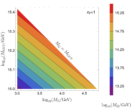
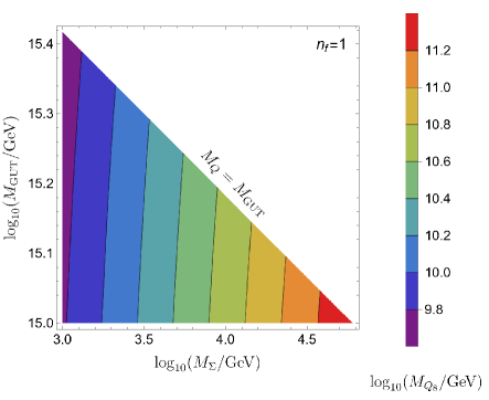
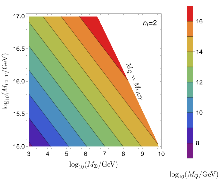
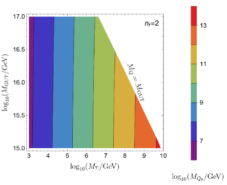
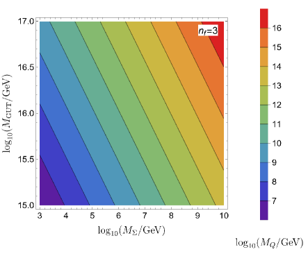
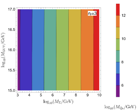
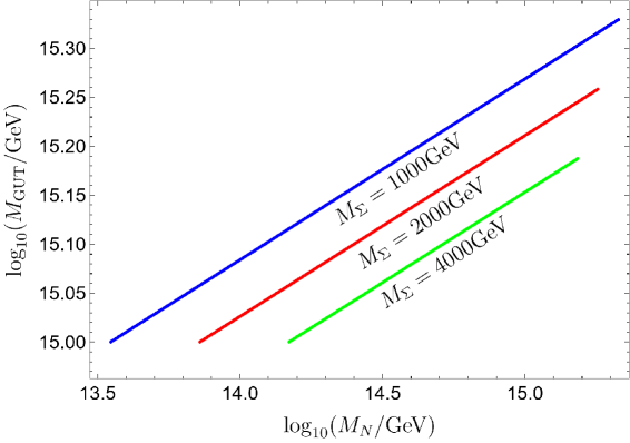
In the gauge space, the SM matter fields belong to - and -plets. In the model, the new matter fields are included in the -plets, the field decomposition from to the SM gauge group and the particles contained in each representation are listed in Table 1. New particles which have contribution to RG equations are . We calculate the coefficients of these new particles in Eq. (32). Using Eq. (47), we obtain the parameter space of and and show the dependence of and upon them. Furthermore, we will set GeV for simplicity while performing scan. This is consistent with the lower bound of heavy leptons set by the collider searches at ATLAS ( GeV at 95% confidence level) [30]. By fixing the copy of at , correlations of these scales are presented in the upper, middle and lower panels of Fig. 1. Here we have assumed masses of all particles in not heavier than such that the theory is always in the perturbative regime. For , degenerate masses between different copies are assumed for illustration. As seen in the plots, the allowed parameter space gradually increases as the copy of increases. When has only one copy (), the maximum value of is about GeV ( GeV), ranges from 1 TeV to 63 TeV under the condition where GeV. This means a strongly fine tuning between , and is required to generate a much smaller value of . In the rest of this work, we only focus on the situation where has only one copy.
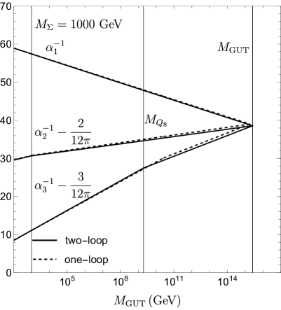
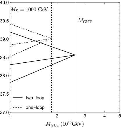
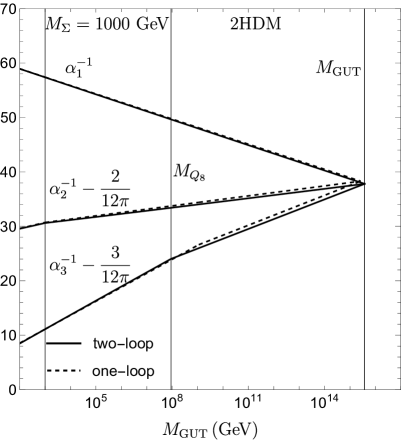
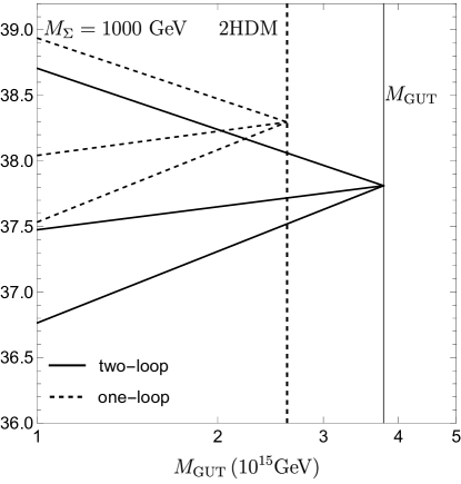
By setting , we further show an example of gauge couplings running respectively at one- and two-loop levels in Fig. 2 with GeV and fixed. As seen in the figure, the two-loop RG running helps to enhance the GUT scale by roughly 40% compared with the one-loop running, namely, GeV at two-loop compared with GeV at one-loop. This enhancement is quantitatively important to obtain the proton lifetime because the latter is proportional to .
Based on the masses of , , and calculated in Eq. (6), first, we assume . Then, we can get the following mass correlation of , , and
| (48) |
Combing it and with the one-loop matching condition in Eq. (47), we obtain GeV, where the maximal value is taken at GeV. This is obviously inconsistent with the current experimental limit.
We consider the general case with . The correlation among , , and masses becomes
| (49) |
Combining with correlations between heavy lepton masses and the GUT scale required by the gauge unification in Fig. 1, is only relevant to and . Setting , we get the relation between and , illustrated in Fig. 3. As we can see, under the condition , the maximal value of is about GeV with GeV. When ranges in GeV, is constrained in GeV. The maximal value of and the range of gets small while gets larger. When GeV, the maximal value of is GeV, which is allowed by gauge unification.
We check the influence of extra higgs doublet on the gauge unification. In our model, it it natural to have both Higgs EW-doublets decomposed from , exist at scales much lower than the intermediate scale . We consider a simple case with two-Higgs-Doublet Model (2HDM) running from the EW scale. Then, the coefficient including the extra doublet Higgs contribution is given by
| (56) |
which is slightly different from those in the SM case. As a comparison to Fig. 2, we show an example of RG running of gauge couplings at two-loop level in Fig. 4 in 2HDM situation, where all inputs keep the same. The maximal value of is increased by approximately a half compared to that in Fig. 2.
4 Fermion masses and mixing
All charged fermion Yukawa coupling matrices can be bilinearly diagonalised by two unitary matrices,
| (57) |
where a hatted matrix represents a diagonal matrix with all non-vanishing entries positive, and and are unitary matrices. Without loss of generality, we will work in the diagonal charged-lepton flavour basis where .
The CKM matrix is defined as . Dismissing the five unphysical phases, the CKM matrix is parametrised as
| (58) |
where . In the numerical calculation below, we will fix values of CKM mixing angles and CP violating phase at
| (59) |
where are obtained by running their experimental best-fit values to the GUT scale [31, 32]. Note that there is a large redundancy of free parameters in the flavour sector.
In the neutrino sector, the Majorana mass matrix for light neutrino is in general a symmetric and complex matrix, which can be diagonalised by a unitary matrix via,
| (60) |
The product gives the PMNS matrix. The latter is parametrised as
| (61) |
up to three unphysical phases. We apply the best-fit values from NuFIT 5.3[33, 34] in the latter numerical calculation,
| (62) |
The two Majorana phases and on the right hand side of Eq. (61) are undetermined. In our model, we only focus on the case with only one copy of , which contributes only two right-handed heavy leptons and for the generation of light neutrino masses. A well-known consequence is that, via the seesaw mechanism, the lightest neutrino is predicted to be massless, namely, in the normal ordering (NO, ) or in the inverted ordering (IO, ) for neutrino masses. Once the lightest neutrino becomes massless, we are left with only one physical Majorana phase, which will be denoted as , for NO or for IO.
We connect the Dirac Yukawa couplings and with the neutrino masses and the mixing angles. In the case with only one copy -plet fermion, the light neutrino mass matrix is simplified into
| (63) |
where a global minus sign is dismissed. Keeping in mind Eq. (60) and in the charged flavour diagonal basis, we apply Casas-Ibarra parametrization [35, 36, 37] and obtain
| (64) |
for the NO, where (for and ) is the entry of the PMNS matrix , and is a complex parameter.
In the above analysis, we have set GeV and ranges in the allowed range consistent with gauge unification, i.e., (, GeV). Then, when ignoring the influence of the Majorana phase , the Yukawa couplings only depend on the complex parameter . It is transparent that the real part of leads to a simple oscillatory nature, the imaginary part of actually affects the size of the couplings most. In Fig. 5, we set and GeV and show the relative size of the Yukawa couplings and as a function of for NO with .
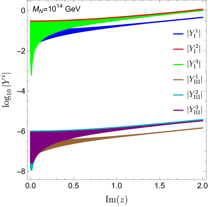
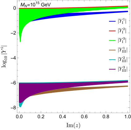
As we can see, is smaller than by a few orders of magnitude due to the large hierarchy between and . When is smaller then 2 (referring to ) or 1 (referring to ), is no more than . In our case, the smallness of three left-handed neutrinos is attributed to the smallness of and the largeness of .
5 Proton decays
The instability of the proton is one of the most attractive predictions of grand unified theories. In this part, our target is to understand if the model satisfies the current proton decay bounds and if it can be tested in future experiments. Partial decay widths of some typical channels of proton decay into a lepton and a meson are given by[38, 39]
| (65) |
Here is the phase space contribution ignoring charged lepton masses,
| (66) |
and parametrising the long-distance and short-distance effect of the baryon-number-violating operators [40], accounting for renormalisation contribution of the QCD running from to the proton mass scale
| (67) |
and that from the GUT scale down to
| (68) |
respectively, where we considered the extra matter at a single intermediate scale and .
The revelant hadronic matrix elements can be obtained by using QCD lattice simulation. We use the best-fit values reported in the recent paper[41], i.e.,
| (69) |
The coefficients appearing in these formulas are [38]
| (70) |
where . There are a large number of free parameters introduced by the unitary matrices. In the above section, we have used a basis where . Even in this case, we still have large redundancies. In the following phenomenological discussion, we will further concentrate on the following three specified scenarios.
-
S1)
Diagonal down-type quark Yukawa couplings, , leading to .
-
S2)
Diagonal up-type quark Yukawa couplings, , leading to .
-
S3)
Hermitian quark Yukawa couplings, and , leading to and .
Detailed discussions on these scenarios are given below.
S1)
In this scenario, we have . is in general different from . Sizes of each entries of satisfy and , where and is the Cabibbo angle. When calculating the coefficients in proton decay lifetime, we consider precision up to the order and ignore smaller quantities. Then, proton partial decay widths can be expressed more straightforwardly,
| (71) |
Obviously, we are left with only two free parameters and , which are relevant to some degrees of freedom associated with the right-handed up-type quark fields. To see more clearly the dependence of proton lifetime upon the parameters, we assume and , values of which are consistent with gauge unification discussed in the last section. The proton partial decay lifetime can be obtained numerically as
| (72) |
where we have used values of CKM matrix elements from Particle Data Group [42]. A short lifetime for is predicted if . Namely, to generate a signal consistent with current data, the unitary matrix must deviates from the diagonal matrix.
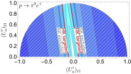
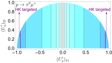
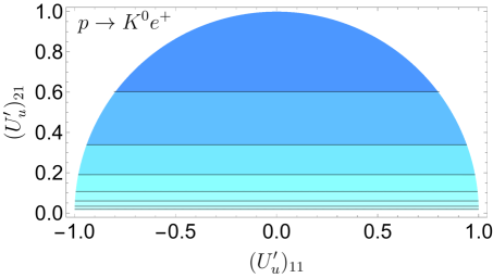
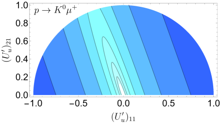
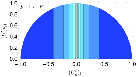
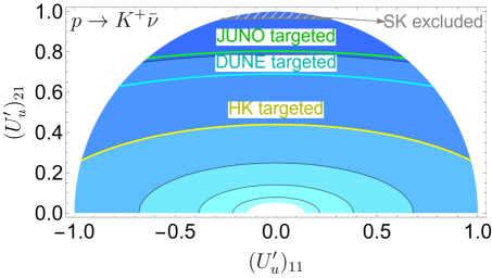

We perform a numerical scan for illustration. and are assumed to be real and and are restricted. The unitarity of requires . An explicit analysis should include a relative phase between and if they are relaxed to be complex. This phase is less important and ignored here. Instead, the positive and negative signs for refer to two extremal cases for the relative phase at 0 and , respectively. Obviously the proton lifetime tends to infinity as tend to zero. Then we show the predictions for the six channels above in Fig. 6. Here, we observe that for the channel, a large range of the parameter space of and is still consistent with the Hyper-Kamiokande (HK) bound. However, most of this range has been excluded in the channel measurement, as expected from the analytical formula in Eq. (5). The prediction of proton decay lifetime for the channel is much longer than the upper bound set by Super-Kamiokande (SK). As we can see, the prediction of proton decay lifetime for the channel is bigger than the limit of SK completely.
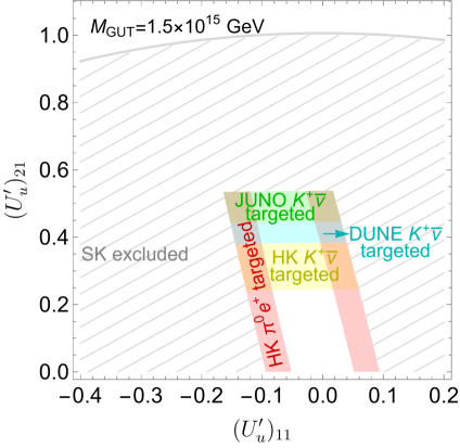
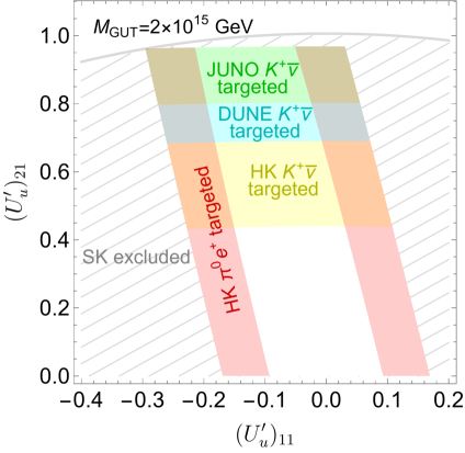
We further check the testability of the the flavour space in light of the JUNO, DUNE and HK experiments. We zoom in Fig. 7 the parameter space of and within the touch of these experiments. The parameter space targeted by HK via the channel is intersected with that targeted by JUNO, DUNE and HK via the channel, but each meaurements all have their own respectively targeted regions. It is notably to menion that as gets larger, the allowed parameter space increases, gets larger and exceeds JUNO’s ability, even exceeds DUNE’s ability. To sum up, there is hope to test this theory in future proton decay experiments, especially in the JUNO, DUNE and HK experiments.
S2)
In S2), we have . in general should be different from . Similar to S1), proton partial decay widths can be written in simple way, e.g.,
| (73) |
The numerical expression of the above equation is
| (74) |
once GeV and GeV are fixed. Here, is just a number which is not relevant to . However, we have checked that the prediction for the channel is always less than years, which is obviously not meeting current limits of SK, years [23]. Therefore, this scenario is excluded.
S3) and
In S3), we have . is a free unitary matrix. Similar to the discussion in S1), we obtain proton partial decay widths here as
| (75) |
In this scenario, four free parameters are involved, , , and . Formulas for and , as well as those for and , are almost the same except the replacements and . and are independent of any entries of . By fixing and , we obtain
| (76) |
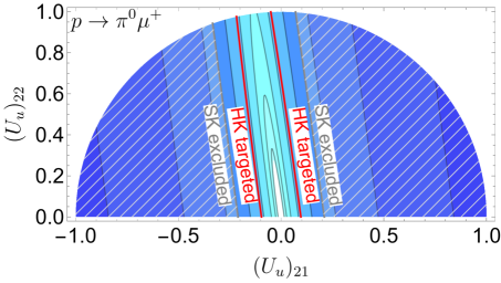
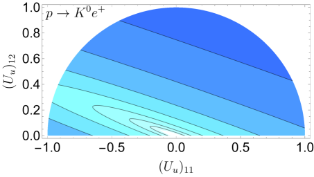
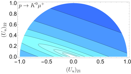
where values of CKM matrix elements have been taken from Particle Data Group(PDG)[42]. We show the dependence of proton partial lifetime upon entries of in Fig. 8. The last two channels, which are independent of , predicts fixed partial lifetime consistent with current SK bounds [44, 24]. In particular, the channel is beyond the future sensitivities of HK [27].

To end this section, we comment on the case with 2HDM. Following the discussion in the end of Section 3, the main effect of including one more Higgs doublet at the electroweak scale is an enhancement of the GUT scale, but not to the flavour space. We expect that, once the GUT scale fixed at the same scale, the restriction on the parameter space of and in Figs. (6) and (7), as well as that of and in Fig. (8), keep almost the same. Assuming a higher GUT scale, e.g., , which are not consistent with SM but 2HDM, a longer proton decay is predicted and the restriction on the flavour space is weaker.
6 Conclusion
We discussed economical extensions of model by including extra fermion multiplets. These multiplets include electroweak singlets and triplets, which may play important roles in light neutrino mass generation through type-I or type-III seesaw mechanisms. Including the fermions saves the gauge unification and predicts proton decay lifetime compatible with current experimental bounds. We focus on the minimal case that only one copy of is introduced. Light neutrino masses are generated via type-(I+III) seesaw and the lightest neutrino keeps massless. The electroweak singlet and triplet fermion are restricted to be around the canonical seesaw scale and TeV scale, respectively. We have checked that all data of lepton flavour mixing can be reproduced, but large hierarchy between Yukawa for and that for has to be included.
We further study contribution of free parameters in the flavour space to different channels of nucleon decays. We have considered three scenarios: S1) down-type quark Yukawa matrix is diagonal; S2) up-quark Yukawa matrix is diagonal; and S3) both Yukawa matrices are Hermitian. In S1), only two free parameters in the flavour space contribute to the proton decay channels we discussed in this work, . Combining and channel for analysis excludes most of the parameter space of S1), but there is still some space for future experiments to test, such as JUNO and HK. S2) predicts a short partial lifetime for and has fully been excluded by SK. In S3), more free parameters are involved in different channels of the nucleon decay, but not to the and channels. With the development of precise experimental measurement in the future, we expect a multi-channel analysis will potentially provide extra information of the flavour space of GUTs that cannot be obtained in the traditional measurements for quark and lepton flavours.
Acknowledgement
This work is supported by National Natural Science Foundation of China (NSFC) under Grants Nos. 12205064, 12347103 and Zhejiang Provincial Natural Science Foundation of China under Grant No. LDQ24A050002.
References
- [1] H. Georgi and S. L. Glashow, Phys. Rev. Lett. 32 (1974), 438-441 doi:10.1103/PhysRevLett.32.438
- [2] J. C. Pati and A. Salam, Phys. Rev. Lett. 31 (1973), 661-664 doi:10.1103/PhysRevLett.31.661
- [3] H. Georgi, H. R. Quinn and S. Weinberg, Phys. Rev. Lett. 33 (1974), 451-454 doi:10.1103/PhysRevLett.33.451
- [4] J. R. Ellis and M. K. Gaillard, Phys. Lett. B 88 (1979), 315-319 doi:10.1016/0370-2693(79)90476-3
- [5] S. Weinberg, Phys. Rev. Lett. 43 (1979), 1566-1570 doi:10.1103/PhysRevLett.43.1566
- [6] Q. Shafi and C. Wetterich, Phys. Rev. Lett. 52 (1984), 875 doi:10.1103/PhysRevLett.52.875
- [7] S. L. Glashow, NATO Sci. Ser. B 61 (1980), 687 doi:10.1007/978-1-4684-7197-7_15
- [8] G. Senjanovic, BNL-29092.
- [9] M. Magg and C. Wetterich, Phys. Lett. B 94 (1980), 61-64 doi:10.1016/0370-2693(80)90825-4
- [10] R. N. Mohapatra and G. Senjanovic, Phys. Rev. D 23 (1981), 165 doi:10.1103/PhysRevD.23.165
- [11] G. Lazarides, Q. Shafi and C. Wetterich, Nucl. Phys. B 181 (1981), 287-300 doi:10.1016/0550-3213(81)90354-0
- [12] B. Bajc and G. Senjanovic, JHEP 08 (2007), 014 doi:10.1088/1126-6708/2007/08/014 [arXiv:hep-ph/0612029 [hep-ph]].
- [13] B. Bajc, M. Nemevsek and G. Senjanovic, Phys. Rev. D 76 (2007), 055011 doi:10.1103/PhysRevD.76.055011 [arXiv:hep-ph/0703080 [hep-ph]].
- [14] I. Dorsner and P. Fileviez Perez, Nucl. Phys. B 723 (2005), 53-76 doi:10.1016/j.nuclphysb.2005.06.016 [arXiv:hep-ph/0504276 [hep-ph]].
- [15] I. Dorsner, P. Fileviez Perez and G. Rodrigo, Phys. Rev. D 75 (2007), 125007 doi:10.1103/PhysRevD.75.125007 [arXiv:hep-ph/0607208 [hep-ph]].
- [16] I. Dorsner and I. Mocioiu, Nucl. Phys. B 796 (2008), 123-136 doi:10.1016/j.nuclphysb.2007.12.004 [arXiv:0708.3332 [hep-ph]].
- [17] L. Di Luzio and L. Mihaila, Phys. Rev. D 87 (2013), 115025 doi:10.1103/PhysRevD.87.115025 [arXiv:1305.2850 [hep-ph]].
- [18] I. Dorsner, S. Fajfer and I. Mustac, Phys. Rev. D 89 (2014) no.11, 115004 doi:10.1103/PhysRevD.89.115004 [arXiv:1401.6870 [hep-ph]].
- [19] P. Fileviez Perez and C. Murgui, Phys. Rev. D 94 (2016) no.7, 075014 doi:10.1103/PhysRevD.94.075014 [arXiv:1604.03377 [hep-ph]].
- [20] C. Hagedorn, T. Ohlsson, S. Riad and M. A. Schmidt, JHEP 09 (2016), 111 doi:10.1007/JHEP09(2016)111 [arXiv:1605.03986 [hep-ph]].
- [21] I. Doršner and S. Saad, Phys. Rev. D 101 (2020) no.1, 015009 doi:10.1103/PhysRevD.101.015009 [arXiv:1910.09008 [hep-ph]].
- [22] G. Senjanović and M. Zantedeschi, Phys. Rev. D 109 (2024) no.9, 095009 doi:10.1103/PhysRevD.109.095009 [arXiv:2402.19224 [hep-ph]].
- [23] A. Takenaka et al. [Super-Kamiokande], Phys. Rev. D 102 (2020) no.11, 112011 doi:10.1103/PhysRevD.102.112011 [arXiv:2010.16098 [hep-ex]].
- [24] V. Takhistov [Super-Kamiokande], [arXiv:1605.03235 [hep-ex]].
- [25] A. Abusleme et al. [JUNO], Chin. Phys. C 47 (2023) no.11, 113002 doi:10.1088/1674-1137/ace9c6 [arXiv:2212.08502 [hep-ex]].
- [26] B. Abi et al. [DUNE], [arXiv:2002.03005 [hep-ex]].
- [27] K. Abe et al. [Hyper-Kamiokande], [arXiv:1805.04163 [physics.ins-det]].
- [28] P. S. B. Dev, L. W. Koerner, S. Saad, S. Antusch, M. Askins, K. S. Babu, J. L. Barrow, J. Chakrabortty, A. de Gouvêa and Z. Djurcic, et al. J. Phys. G 51 (2024) no.3, 033001 doi:10.1088/1361-6471/ad1658 [arXiv:2203.08771 [hep-ex]].
- [29] S. F. King, S. Pascoli, J. Turner and Y. L. Zhou, JHEP 10 (2021), 225 doi:10.1007/JHEP10(2021)225 [arXiv:2106.15634 [hep-ph]].
- [30] G. Aad et al. [ATLAS], Eur. Phys. J. C 82 (2022) no.11, 988 doi:10.1140/epjc/s10052-022-10785-0 [arXiv:2202.02039 [hep-ex]].
- [31] S. Antusch and V. Maurer, JHEP 11 (2013), 115 doi:10.1007/JHEP11(2013)115 [arXiv:1306.6879 [hep-ph]].
- [32] K. S. Babu, B. Bajc and S. Saad, JHEP 02 (2017), 136 doi:10.1007/JHEP02(2017)136 [arXiv:1612.04329 [hep-ph]].
- [33] I. Esteban, M. C. Gonzalez-Garcia, M. Maltoni, T. Schwetz and A. Zhou, JHEP 09 (2020), 178 doi:10.1007/JHEP09(2020)178 [arXiv:2007.14792 [hep-ph]].
- [34] NuFIT 5.3 (2024), http://www.nu-fit.org/?q=node/278
- [35] J. A. Casas and A. Ibarra, Nucl. Phys. B 618 (2001), 171-204 doi:10.1016/S0550-3213(01)00475-8 [arXiv:hep-ph/0103065 [hep-ph]].
- [36] A. Ibarra and G. G. Ross, Phys. Lett. B 591 (2004), 285-296 doi:10.1016/j.physletb.2004.04.037 [arXiv:hep-ph/0312138 [hep-ph]].
- [37] A. Arhrib, R. Benbrik and C. H. Chen, Phys. Rev. D 81 (2010), 113003 doi:10.1103/PhysRevD.81.113003 [arXiv:0903.1553 [hep-ph]].
- [38] P. Fileviez Perez, Phys. Lett. B 595 (2004), 476-483 doi:10.1016/j.physletb.2004.06.061 [arXiv:hep-ph/0403286 [hep-ph]].
- [39] P. Fileviez Pérez, A. Gross and C. Murgui, Phys. Rev. D 98 (2018) no.3, 035032 doi:10.1103/PhysRevD.98.035032 [arXiv:1804.07831 [hep-ph]].
- [40] P. Nath and P. Fileviez Perez, Phys. Rept. 441 (2007), 191-317 doi:10.1016/j.physrep.2007.02.010 [arXiv:hep-ph/0601023 [hep-ph]].
- [41] Y. Aoki, T. Izubuchi, E. Shintani and A. Soni, Phys. Rev. D 96 (2017) no.1, 014506 doi:10.1103/PhysRevD.96.014506 [arXiv:1705.01338 [hep-lat]].
- [42] R. L. Workman et al. [Particle Data Group], PTEP 2022 (2022), 083C01 doi:10.1093/ptep/ptac097
- [43] R. Matsumoto et al. [Super-Kamiokande], Phys. Rev. D 106 (2022) no.7, 072003 doi:10.1103/PhysRevD.106.072003 [arXiv:2208.13188 [hep-ex]].
- [44] K. Abe et al. [Super-Kamiokande], Phys. Rev. Lett. 113 (2014) no.12, 121802 doi:10.1103/PhysRevLett.113.121802 [arXiv:1305.4391 [hep-ex]].
- [45] M. Yokoyama [Hyper-Kamiokande Proto], [arXiv:1705.00306 [hep-ex]].
- [46] K. Kobayashi et al. [Super-Kamiokande], Phys. Rev. D 72 (2005), 052007 doi:10.1103/PhysRevD.72.052007 [arXiv:hep-ex/0502026 [hep-ex]].