Cluster GARCH

Abstract

We introduce a novel multivariate GARCH model with flexible convolution-$t$ distributions that is applicable in high-dimensional systems. The model is called Cluster GARCH because it can accommodate cluster structures in the conditional correlation matrix and in the tail dependencies. The expressions for the log-likelihood function and its derivatives are tractable, and the latter facilitate a score-drive model for the dynamic correlation structure. We apply the Cluster GARCH model to daily returns for 100 assets and find it outperforms existing models, both in-sample and out-of-sample. Moreover, the convolution-$t$ distribution provides a better empirical performance than the conventional multivariate $t$-distribution.

Keywords: Multivariate GARCH, Score-Driven Model, Cluster Structure, Block Correlation Matrix, Heavy Tailed Distributions.

JEL Classification: G11, G17, C32, C58

1 Introduction

Univariate GARCH models have enjoyed considerable empirical success since they were introduced in Engle, (1982) and refined in Bollerslev, (1986). In contrast, the success of multivariate GARCH models has been more moderate due to a number of challenges, see e.g. Bauwens et al., (2006). A common approach to modeling covariance matrices is to model variances and correlations separately, as is the case in the Constant Conditional Correlation (CCC) model by Bollerslev, (1990) and the Dynamic Conditional Correlation (DCC) model by Engle, (2002). See also Engle and Sheppard, (2001), Tse and Tsui, (2002), Aielli, (2013), Engle et al., (2019), and Pakel et al., (2021). While univariate conditional variances can be effectively modeled using standard GARCH models, the modeling of dynamic conditional correlation matrices necessitates less intuitive choices to be made. One challenge is that the number of correlations increases with the square of the number of variables, a second challenge is that the conditional correlation matrix must be positive semidefinite, and a third challenge is to determine how correlations should be updated in response to sample information.

In this paper, we develop a novel dynamic model of the conditional correlation matrix, the Cluster GARCH model, which has three main features. First, use convolution-$t$ distributions, which is a flexible class of multivariate heavy-tailed distributions with tractable likelihood expressions. The multivariate $t$-distributions are nested in this framework, but a convolution-$t$ distribution can have heterogeneous marginal distributions and cluster-based dependencies. For instance, convolution-$t$ distributions can generate the type of sector-specific price jumps reported in Andersen et al., (2024). Second, the dynamic model is based on the score-driven framework by Creal et al., (2013), which leads to closed-form expressions for all key quantities. Third, the model can be combined with a block correlation structure that makes the model applicable to high-dimensional systems. This partitioning, defining the block structure, can also be interpreted as a second type of cluster structure.

Heavy-tailed distributions are common in financial returns, and many empirical studies adopt the multivariate $t$-distribution to model vectors of financial series, e.g., Kotz and Nadarajah, (2004), Harvey, (2013), and Ibragimov et al., (2015). An implication of the multivariate $t$-distribution is that all standardized returns have identical and time-invariant marginal distributions. This is a restrictive assumption, especially in high dimensions. The convolution-$t$ distributions by Hansen and Tong, (2024) relax these assumptions, and one of the main contributions of this paper is to incorporate this class of distributions into a tractable multivariate GARCH model. A convolution-$t$ distribution is a convolution of multivariate $t$-distributions. In the Cluster GARCH model, standardized returns are time-varying linear combinations of independent $t$-distributions, which can have different degrees of freedom. This leads to dynamic and heterogeneous marginal distributions for standardized returns, albeit the conventional multivariate $t$-distribution is nested in this framework as a special case. We focus on three particular types of convolution-$t$ distributions, labelled Canonical-Block-$t$, Cluster-$t$, and Hetero-$t$. These all have relatively simple log-likelihood functions, such that we can obtain closed-form expressions for the first two derivatives, score and information matrix, of the conditional log-likelihood functions. These are used in our score-driven model for the time-varying correlation structure, which is a key component of the Cluster GARCH model.

High-dimensional correlation matrices can be modeled using a parsimonious block structure for the conditional correlation matrix. The DCC model is parsimonious but greatly limits the way the conditional covariance matrix can be updated. Without additional structure, the number of latent variables increases with $n^{2}$, where $n$ is the number of assets. This number becomes unmanageable once $n$ is more than a single digit, and maintaining a positive definite correlation matrix can be challenging too. The correlation structure in the Block DECO model by Engle and Kelly, (2012) is an effective way to reduce the dimension of the estimated parameters. However, the estimation strategy in Engle and Kelly, (2012) was based on an ad-hoc averaging of within-block correlations for an auxiliary DCC model, and they did not fully utilize the simplifications offered by the block structure. The model proposed in this paper draws on recent advances in correlation matrix analysis by Archakov and Hansen, (2021, 2024). We will, in some specifications, adopt the block parameterization of the conditional correlation matrix, used in Archakov et al., (2020), which has (at most) $K\left(K+1\right)/2$ free parameters where $K$ is the number of blocks. This approach guarantees a positive definite correlation matrix and the likelihood evaluation is greatly simplified. Overall, the Cluster GARCH offers a good balance between flexibility and computational feasibility in high dimensions.

We adopt the convenient parametrization of the conditional correlation matrix, $\gamma(C)$, which is defined by taking the matrix logarithm of the correlation matrix, $C$, and stacking the off-diagonal elements of $\log C$ into the vector, $\gamma\in\mathbb{R}^{d}$, where $d=n(n-1)/2$. This parametrization was introduced in Archakov and Hansen, (2021) and the mapping $C\mapsto\gamma(C)$ is one-to-one between the set of non-singular correlation matrices $\mathcal{C}_{n\times n}$ and $\mathbb{R}^{d}$. So, the inverse mapping, $C(\gamma)$, will always yield a positive definite correlation matrix and any non-singular correlation matrix can be generated in this way. The parametrization can be viewed as a generalization of Fisher’s Z-transformation to the multivariate case. It has attractive finite sample properties, which makes it suitable for an autoregressive model structure, see Archakov and Hansen, (2021).

A block correlation structure arises when variables can be partitioned into clusters, $K$ say, and the correlation between two variables is determined by their cluster assignments. When $C$ has a block structure, then $\log C$ also has a block structure. This leads to a new parametrization of block correlation matrices, which defines a one-to-one mapping $C\mapsto\eta(C)$ between the set of non-singular block correlation matrices $\mathcal{C}_{n\times n}$ and $\mathbb{R}^{d}$ with $d=K\left(K+1\right)/2$. We adopt the canonical representation by Archakov and Hansen, (2024), which is a quasi-spectral decomposition of block matrices that diagonalizes the matrix with the exception of a small $K\times K$ submatrix. This decomposition makes the model parsimonious and greatly simplifies the evaluations of the log-likelihood function. This parameterization of block correlation matrices is more general than the factor-based approach to parametrizing block correlation matrices.

Our paper contributes to the literature on score-driven model for dynamics of covariance matrices. Using the multivariate $t$-distribution, Creal et al., (2012) and Hafner and Wang, (2023) proposed score-driven model for time-varying covariance and correlation matrix, respectively. Oh and Patton, (2023) proposed a score-driven dynamic factor copula models with skew-$t$ copula function, however, the analytical information matrices in these copula models are not available. Using realized measures of the covariance matrix, Gorgi et al., (2019) proposed the Realized Wishart-GARCH, which relies on a Wishart distribution for realized covariance matrices and on a Gaussian distribution for returns. Opschoor et al., (2017) constructed a multivariate HEAVY model based on Heavy-tailed distributions for both returns and the realized covariances. An aspect, which sets the Cluster GARCH apart from the existing literature, is that the model is based on the convolution-$t$ distributions, which includes the Gaussian distribution and the multivariate $t$-distributions as special cases. The block structures we impose on the correlation matrix in some specifications, was previously used in Archakov et al., (2020). Their model used the Realized GARCH framework with a Gaussian specification, whereas we adopt the score-driven framework for convolution-$t$ distributions, and do require realized volatility measures in the modeling.

We conduct an extensive empirical investigation on the performance of our dynamic model for correlation matrices. The sample period spans the period from January 3, 2005 to December 31, 2021. The new model is applicable to high dimensions, and we consider a “small universe” with $n=9$ assets and a “large universe” with $n=100$ assets. The small universe allows us compare the new models with a range of existing models, as most of these are not applicable to the large universe. We also undertake an more detailed specification analysis with the small universe. The nine stocks are from three sectors, three from each sector, which motivates certain block and cluster structures. First, we find that the convolution-$t$ distribution offers a better fit than the conventional $t$-distribution. Overall, the Cluster-$t$ distribution has the largest log-likelihood value. Second, we find that score-driven models successfully captures the dynamic variation in the conditional correlation matrix. The new score-driven models outperform traditional DCC models when based on the same distributional assumptions, and the proposed score-driven model with a sector motivated block correlation matrix has the smallest BIC.

The large universe with $n=100$ stocks poses no obstacles for the Cluster GARCH model. We used the sector classification of the stocks to define the block structure in the correlation matrix. We also used the sector classification to explore possible cluster structures in the tail-dependencies, which are related to parameters in the convolution-$t$ distribution. With $K=10$ sectors this reduces the number of free parameters in the correlation matrix from 4950 to 55, and the model estimation is very fast and stable, in part because the required computations only involve $K\times K$ matrices (instead of $n\times n$ matrices). For the large universe, the empirical results favor the Hetero-$t$ specification, which entails a convolutions of a large number of univariate $t$-distributions. We also find that correlation targeting, which is analogous to variance targeting in GARCH models, is beneficial.

The rest of this paper is organized as follows: In Section 2 we introduce a new parametrization of block correlation matrices, based on Archakov and Hansen, (2021) and Archakov and Hansen, (2024). In Section 3, we introduce the convolution-$t$ distributions. We derive the score-driven models in Section 4, and we obtain analytical expressions for the score and information matrix for the convolution-$t$ distributions, including the special case where $C$ has a block structure. Some details about practical implementation are given in Section 5. The empirical analysis is presented in Section 6 and includes in-sample and out-of-sample evaluations and comparisons. All proofs are given in the Appendix.

2 The Theoretical Model

Consider an $n$-dimensional time-series, $R_{t}$, $t=1,2,\ldots,T$, and let $\{\mathcal{F}_{t}\}$ be a filtration to which $R_{t}$ is adapted, i.e. $R_{t}\in\mathcal{F}_{t}$. We denote the conditional mean by $\mu_{t}=\mathbb{E}(R_{t}|\mathcal{F}_{t-1})$ and the conditional covariance matrix by $\Sigma_{t}=\mathrm{var}(R_{t}|\mathcal{F}_{t-1})$. With $\Lambda_{\sigma_{t}}\equiv\mathrm{diag}(\sigma_{1t},\ldots,\sigma_{nt})$, where $\sigma_{it}^{2}=\mathrm{var}(R_{it}|\mathcal{F}_{t-1})$, $i=1,\ldots,n$, it follows that the conditional correlation matrix is given by

$$C_{t}=\Lambda_{\sigma_{t}}^{-1}\Sigma_{t}\Lambda_{\sigma_{t}}^{-1}.$$

Initially, we take $\mu_{t}$ and $\Lambda_{\sigma_{t}}$ as given and focus on the dynamic modeling of $C_{t}$. We are particularly interested in the case where $n$ is large. We define the following standardized variables with a dynamic correlation matrix $C_{t}$,

$$Z_{t}=\Lambda_{\sigma_{t}}^{-1}(X_{t}-\mu_{t}).$$

To simplify the notation, we omit subscript-$t$ in most of Sections 2 and 3 and reintroduce it again in Section 4 where the dynamic model is presented.

2.1 Block Correlation Matrix

If $n$ is relatively small, we can model the dynamic correlation matrix using $d=n(n-1)/2$ latent variables. Additional structure on $C$ is required when $n$ is larger, because the number of latent variables becomes unmanageable. Additional structure can be imposed using a block structures on $C$, as in Engle and Kelly, (2012).

A block correlation matrix is characterized by a partitioning of the variables into clusters, such that the correlation between two variables is solely determined by their cluster assignments. Let $K$ be the number of clusters, and let $n_{k}$ be the number of variables in the $k$-th cluster, $k=1,\ldots,K$, such that $n=\sum_{k=1}^{K}n_{k}$. We let $\bm{n}=\left(n_{1},n_{2},\ldots,n_{K}\right)^{\prime}$ be the vector with cluster sizes and sort the variables such that the first $n_{1}$ variables are those in the first cluster , the next $n_{2}$ variables are those in the second cluster, and so forth. Then $C=\mathrm{corr}(Z)$ will have the following block structure

$$C=\left[\begin{array}[]{cccc}C_{[1,1]}&C_{[1,2]}&\cdots&C_{[1,K]}\\ C_{[2,1]}&C_{[2,2]}\\ \vdots&&\ddots\\ C_{[K,1]}&&&C_{[K,K]}\end{array}\right],$$ (1)

where $C_{[k,l]}$ is an $n_{k}\times n_{l}$ matrix given by

$$C_{[k,l]}=\left[\begin{array}[]{ccc}\rho_{kl}&\cdots&\rho_{kl}\\ \vdots&\ddots&\vdots\\ \rho_{kl}&\cdots&\rho_{kl}\end{array}\right],\text{ for }k\neq l\qquad\text{and }C_{[k,k]}=\left[\begin{array}[]{cccc}1&\rho_{kk}&\cdots&\rho_{kk}\\ \rho_{kk}&1&\ddots\\ \vdots&\ddots&\ddots\\ \rho_{kk}&&&1\end{array}\right].$$

Each block, $C_{[k,l]}$, has just one correlation coefficient, such that the block structure reduces the number of unique correlations from $n\left(n-1\right)/2$ to at most $K\left(K+1\right)/2$. This number does not increase with $n$, and this makes it possible to scale the model to accommodate high-dimensional correlation matrices.

Below we derive score-driven models for unrestricted correlation matrices and for the case where $C$ has a block structure. time].

2.2 Parametrizing the Correlation Matrix

We parameterize the correlation matrix with the vector

$$\gamma(C)\equiv{\rm vecl}\left(\log C\right)\in\mathbb{R}^{d},\qquad d=n(n-1)/2,$$ (2)

where ${\rm vecl}(\cdot)$ extracts and vectorizes the elements below the diagonal and $\log C$ is the matrix logarithm of the correlation matrix. The following example illustrates this parametrization for an $3\times 3$ correlation matrix:

$${\rm vecl}\left[\log\left(\begin{array}[]{ccc}1.0&\bullet&\bullet\\ 0.5&1.0&\bullet\\ 0.3&0.7&1.0\end{array}\right)\right]={\rm vecl}\left[\left(\begin{array}[]{ccc}-0.15&\phantom{-}\bullet&\phantom{-}\bullet\\ \phantom{-}0.53&-0.47&\phantom{-}\bullet\\ \phantom{-}0.13&\phantom{-}0.85&-0.34\end{array}\right)\right]=\left(\begin{array}[]{c}0.53\\ 0.13\\ 0.85\end{array}\right)=:\gamma.$$

This parametrization is convenient because it guarantees a unique positive definiteness correlation matrix, $C(\gamma)$ for any vector $\gamma,$ without imposing superfluous restrictions on the correlation matrix, see Archakov and Hansen, (2021).

For a block correlation matrix the logarithmic transformation preserves the block structure as illustrated in the following example:

$$\underbrace{\left[\begin{array}[]{ccccccc}\pagecolor{black!10}1.0&\pagecolor{black!10}0.8&0.4&0.4&\pagecolor{black!05}0.2&\pagecolor{black!05}0.2&\pagecolor{black!05}0.2\\ \pagecolor{black!10}0.8&\pagecolor{black!10}1.0&0.4&0.4&\pagecolor{black!05}0.2&\pagecolor{black!05}0.2&\pagecolor{black!05}0.2\\ 0.4&0.4&\pagecolor{black!10}1.0&\pagecolor{black!10}0.6&0.1&0.1&0.1\\ 0.4&0.4&\pagecolor{black!10}0.6&\pagecolor{black!10}1.0&0.1&0.1&0.1\\ \pagecolor{black!05}0.2&\pagecolor{black!05}0.2&0.1&0.1&\pagecolor{black!10}1.0&\pagecolor{black!10}0.3&\pagecolor{black!10}0.3\\ \pagecolor{black!05}0.2&\pagecolor{black!05}0.2&0.1&0.1&\pagecolor{black!10}0.3&\pagecolor{black!10}1.0&\pagecolor{black!10}0.3\\ \pagecolor{black!05}0.2&\pagecolor{black!05}0.2&0.1&0.1&\pagecolor{black!10}0.3&\pagecolor{black!10}0.3&\pagecolor{black!10}1.0\end{array}\right]}_{=C}\quad\underbrace{\left[\begin{array}[]{ccccccc}\pagecolor{black!10}-.59&\pagecolor{black!10}1.02&.251&.251&\pagecolor{black!05}.115&\pagecolor{black!05}.115&\pagecolor{black!05}.115\\ \pagecolor{black!10}1.02&\pagecolor{black!10}-.59&.251&.251&\pagecolor{black!05}.115&\pagecolor{black!05}.115&\pagecolor{black!05}.115\\ .251&.251&\pagecolor{black!10}-.29&\pagecolor{black!10}.626&.036&.036&.036\\ .251&.251&\pagecolor{black!10}.626&\pagecolor{black!10}-.29&.036&.036&.036\\ \pagecolor{black!05}.115&\pagecolor{black!05}.115&.036&.036&\pagecolor{black!10}-.09&\pagecolor{black!10}.259&\pagecolor{black!10}.259\\ \pagecolor{black!05}.115&\pagecolor{black!05}.115&.036&.036&\pagecolor{black!10}.259&\pagecolor{black!10}-.09&\pagecolor{black!10}.259\\ \pagecolor{black!05}.115&\pagecolor{black!05}.115&.036&.036&\pagecolor{black!10}.259&\pagecolor{black!10}.259&\pagecolor{black!10}-.09\end{array}\right]}_{=\log C}.$$

The parameter vector, $\gamma$ will only have as many unique elements as there are different blocks in $C$. This number is $(K+1)K/2$, and we can therefore condense $\gamma$ into a subvector, $\eta$, such that

$$\gamma=B\eta,$$ (3)

where $B$ is a known bit-matrix with a single one in each row and $\eta\in\mathbb{R}^{K(K+1)/2}$. This factor structure for $\gamma$ was first proposed in Archakov et al., (2020).

For later use, we define the condensed log-correlation matrix, $\tilde{C}\in\mathbb{R}^{K\times K}$, whose $(k,l$)-th element is the off-diagonal element from the $(k,l)$-th block of $\log C$, $k,l=1,\ldots,K$, and we can set $\eta=\mathrm{vech}(\tilde{C})\in\mathbb{R}^{K(K+1)/2}$. In the example above, we have

$$\tilde{C}=\left[\begin{array}[]{ccc}\pagecolor{black!10}1.02&.251&\pagecolor{black!05}.115\\ .251&\pagecolor{black!10}.626&.036\\ \pagecolor{black!05}.115&.036&\pagecolor{black!10}.259\end{array}\right],$$

such that $\eta=\left[1.02,0.251,0.115,0.626,0.036,0.259\right]^{\prime}$ has dimension six whereas $\gamma$ has dimension 21. Since the block correlation matrix, $C$, is only a function of $\eta$ we can model the time-variation in $C$ using a dynamic model for the unrestricted vector $\eta$. This will be our approach below.

2.3 Canonical Form for the Block Correlation Matrix

Block matrices has a canonical representation that resembles the eigendecomposition of matrices, see Archakov and Hansen, (2024). For a block correlation matrix with block-sizes, $(n_{1},\ldots,n_{K})$, we have

$$C=QDQ^{\prime},\quad D=\left[\begin{array}[]{cccc}A&0&\cdots&0\\ 0&\lambda_{1}I_{n_{1}-1}&\ddots&\vdots\\ \vdots&\ddots&\ddots&0\\ 0&\cdots&0&\lambda_{K}I_{n_{K}-1}\end{array}\right],\quad\lambda_{k}=\frac{n_{k}-A_{kk}}{n_{k}-1},$$ (4)

where the upper left block, $A$, is an $K\times K$ matrix with elements $A_{kl}=\rho_{kl}\sqrt{n_{k}n_{l}}$, for $k\neq l,$and $A_{kk}=1+\left(n_{k}-1\right)\rho_{kk}$. The matrix $Q$ is a group-specific orthonormal matrix, i.e., $Q^{\prime}Q=QQ^{\prime}=I_{n}$. Importantly, $Q$ is solely determined by the block sizes, $(n_{1},\ldots,n_{K})$, and does not depend on the elements in $C$. This matrix is given by

$$Q=\left[\begin{array}[]{cccccccc}v_{n_{1}}&0&\cdots&&v_{n_{1}}^{\perp}&0&\cdots&0\\ 0&v_{n_{2}}&&&0&v_{n_{2}}^{\perp}&&\vdots\\ \vdots&&\ddots&&&&\ddots\\ 0&\cdots&&v_{n_{K}}&0&\cdots&&v_{n_{K}}^{\perp}\end{array}\right],$$

where $v_{n_{k}}=(1/\sqrt{n_{k}},\ldots,1/\sqrt{n_{k}})^{\prime}\in\mathbb{R}^{n_{k}}$ and $v_{n_{k}}^{\perp}$ is an $n_{k}\times(n_{k}-1)$ matrix, which is orthogonal to $v_{n_{k}}$, i.e., $v_{n_{k}}^{\prime}v_{n_{k}}^{\perp}=0$, and orthonormal, such that $v_{n_{k}}^{\perp\prime}v_{n_{k}}^{\perp}=I_{n_{k}-1}.$ The canonical representation enables us to rotate $Z$ with $Q$ and define

$$Y=Q^{\prime}Z,\qquad\text{with }\quad Y=(Y_{0}^{\prime},Y_{1}^{\prime},\ldots,Y_{K}^{\prime})^{\prime},$$ (5)

where $Y_{0}$ is $K$-dimensional with ${\rm var}(Y_{0})=A$, and $Y_{k}$ is $n_{k}-1$ dimensional with ${\rm var}(Y_{k})=\lambda_{k}I_{n_{k}-1}$ for $k=1,\ldots,K$. The block-diagonal structure of $D$ implies that $Y_{0},Y_{1},\ldots$, and $Y_{K}$ are uncorrelated, which simplifies several expressions. For instance, we have the following identities:

$$|C|=|A|\cdot\prod_{k=1}^{K}\lambda_{k}^{n_{k}-1},\quad Z^{\prime}C^{-1}Z=Y_{0}^{\prime}A^{-1}Y_{0}+\sum_{k=1}^{K}\lambda_{k}^{-1}Y_{k}^{\prime}Y_{k},$$ (6)

such that the computation of the determinant and any power of $C$ is greatly simplified. The square-root of the $n\times n$ correlation matrix, $C^{1/2}$, is straight forward to compute. From the eigendecomposition of $A$, $A=P\Lambda_{a}P^{\prime}$, we define the block diagonal matrix: $D^{1/2}=\mathrm{diag}(P\Lambda_{a}^{1/2}P^{\prime},\lambda_{1}^{1/2}I_{n_{1}-1},\ldots,\lambda_{K}^{1/2}I_{n_{K}-1})$, and set $C^{1/2}\equiv QD^{1/2}Q^{\prime}$. It is easy to verify that $C=C^{1/2}C^{1/2}$ and that $C^{1/2}$ is symmetric. Computing $C^{1/2}$ therefore only requires an eigendecomposition of the symmetric and positive definite $K\times K$ matrix, $A$, rather than the eigendecomposition of $C$, which is $n\times n$. Computing other power of $C$ can be done similarly.

We can use Archakov and Hansen, (2024, corollary 2) to recover the elements of the condensed log-correlation matrix,

$$\tilde{C}=\Lambda_{n}^{-1}W\Lambda_{n}^{-1},\quad W=\log A-\log\Lambda_{\lambda},$$

where

$$\Lambda_{\lambda}=\left[\begin{array}[]{ccc}\lambda_{1}&\cdots&0\\ \vdots&\ddots&\vdots\\ 0&\cdots&\lambda_{K}\end{array}\right],\qquad\text{and}\qquad\Lambda_{n}=\left[\begin{array}[]{ccc}\sqrt{n_{1}}&&0\\ &\ddots\\ 0&&\sqrt{n_{K}}\end{array}\right].$$

The unique values in $\tilde{C}$, which are the elements in $\eta$, can be expressed as

$$\eta={\rm vech}(\tilde{C})=L_{K}\left(\Lambda_{n}^{-1}\otimes\Lambda_{n}^{-1}\right){\rm vec}(W),$$

where $L_{K}$ is the elimination matrix, that solves $\mathrm{vech}(A)=L_{k}\mathrm{vec}(A)$. This parametrization of block correlation matrices does not impose additional superfluous restrictions, and the canonical representation facilitates simple computation of the determinant, the matrix inverse, and any other power, as well as the matrix logarithm and the matrix exponential. This is very useful for the evaluation of the likelihood function, especially for the more complicated models with heterogeneous heavy tails and complex dependencies, which we pursue in the next section.

3 Distributions

The next step is to specify a distribution for the $n$-dimensional random vector $Z$, from which the log-likelihood function, $\ell$, is defined. We consider several specifications, ranging from the multivariate normal distribution to convolutions of multivariate $t$-distributions. The convolution-$t$ distributions by Hansen and Tong, (2024) have simple log-likelihood functions and the canonical representation of a block correlation matrix motivates some particular specifications of the convolution-$t$ distribution.

We define

$$U=C^{-1/2}Z,$$

such that $\mathrm{var}(U)=I_{n}$, and a convenient property of any log-likelihood function, $\ell$, is that

$$\ell\left(Z\right)=-\tfrac{1}{2}\log|C|+\ell\left(U\right).$$ (7)

This shows that the log-likelihood function will be in closed-form if we adopt a distribution for $U$ with a closed-form expression for $\ell(U)$, and this is important for obtaining tractable score-driven models. It is well known that the multivariate $t$-distribution and the Gaussian distribution have simple expression for $\ell(U)$. Fortunately, so does the multivariate convolution-$t$ distributions, which has different and interesting statistical properties for $Z$.

3.1 Multivariate $t$-Distributions

We begin with the simplest heavy-tailed distribution, a scaled multivariate $t$-distribution, which nests the Gaussian distribution as a limited case. The multivariate $t$-distribution is widely used to model vectors of returns with heavy tailed distributions, see e.g. Creal et al., (2012), Opschoor et al., (2017), and Hafner and Wang, (2023).

The $n$-dimensional multivariate $t$-distribution with $\nu$ degrees of freedom, location $\mu\in\mathbb{R}^{n}$, and scale matrix $\Sigma\in\mathbb{R}^{n\times n}$, typically written $X\sim t_{\nu}(\mu,\Sigma)$, has density

$$f_{X}(x)=\tfrac{\Gamma(\tfrac{\nu+n}{2})}{\Gamma(\tfrac{\nu}{2})}[\nu\pi]^{-\frac{n}{2}}|\Sigma|^{-\frac{1}{2}}\left[1+\tfrac{1}{\nu}(x-\mu)^{\prime}\Sigma^{-1}(x-\mu)\right]^{-\frac{\nu+n}{2}}.$$

The variance is well-defined when $\nu>2$, in which case $\mathrm{var}(X)=\tfrac{\nu}{\nu-2}\Sigma$. The parameter $\nu$ governs the heaviness of the tail and the multivariate $t$-distribution converges to the multivariate normal distribution, $N(\mu,\Sigma)$, as $\nu\rightarrow\infty$.

To simplify the notation, we will use a scaled multivariate $t$-distribution, denoted $t_{\nu}^{\mathrm{std}}(0,\Sigma)$, which is defined for $\nu>2$. Its density is given by,

$$f_{Y}(y)=\tfrac{\Gamma(\tfrac{\nu+n}{2})}{\Gamma(\tfrac{\nu}{2})}[(\nu-2)\pi]^{-\frac{n}{2}}|\Sigma|^{-\frac{1}{2}}\left[1+\tfrac{1}{\nu-2}y{}^{\prime}\Sigma^{-1}y\right]^{-\frac{\nu+n}{2}},\qquad\nu>2.$$ (8)

The relation between the two distributions is as follows: If $X\sim t_{\nu}(0,\Sigma)$ with $\nu>2$, then $Y=\sqrt{\tfrac{\nu-2}{\nu}}X\sim t_{\nu}^{\mathrm{std}}(0,\Sigma)$. The main advantage of the scaled $t$-distribution is that $\mathrm{var}(Y)=\Sigma$. Thus, if $U\sim t_{\nu}^{\mathrm{std}}(0,I_{n})$ then $Z=C^{1/2}U\sim t_{\nu}^{\mathrm{std}}(0,C)$, and the corresponding log-likelihood function is given by

$$\ell(Z)=c(\nu,n)-\tfrac{1}{2}\log|C|-\tfrac{\nu+n}{2}\log\left(1+\tfrac{1}{\nu-2}Z^{\prime}C^{-1}Z\right),$$ (9)

where $c(\nu,n)=\log\left(\Gamma(\tfrac{\nu+n}{2})/\Gamma(\tfrac{\nu}{2})\right)-\frac{n}{2}\log\left[\left(\nu-2\right)\pi\right]$ is a normalizing constant that does not depend on the correlation matrix, $C$. If $C$ has a block structure we can use the identities in (6), and obtain the following simplified expression,

$$\ell(Z)= c(\nu,n)-\tfrac{1}{2}\log|A|-\tfrac{1}{2}\sum_{k=1}^{K}\left(n_{k}-1\right)\log\lambda_{k}$$ (10)

$$-\tfrac{\nu+n}{2}\log\left(1+\tfrac{1}{\nu-2}\left(Y_{0}^{\prime}A^{-1}Y_{0}+\sum_{k=1}^{K}\lambda_{k}^{-1}Y_{k}^{\prime}Y_{k}\right)\right).$$

The multivariate $t$-distribution has two implications for all elements of the vector $Z$. First, all elements of a multivariate $t$-distribution are dependent, because they share a common random mixing variable. Second, all elements of $U$ are identically distributed, because they are $t$-distributed with the same degrees of freedom. Both implications may be too restrictive in many applications, especially if the dimension, $n$, is large. Below we consider the convolution-$t$ distribution proposed in Hansen and Tong, (2024), which allows for heterogeneity and cluster structures in the tail properties and the tail dependencies.

3.2 Multivariate Convolution-$t$ Distributions

The multivariate convolution-$t$ distribution is a suitable rotations of a random vector that is made up of independent multivariate $t$-distributions. More specific, let $V_{1},\ldots,V_{G}$ be mutually independent standardized multivariate $t$-distributed variables, $V_{g}\sim t_{\nu_{g}}^{\mathrm{std}}(0,I_{m_{g}})$, with $\nu_{g}>2$ for all $g=1,\ldots,G$ and $n=\sum_{g=1}^{G}m_{g}$.

Then $V=(V_{1}^{\prime},\ldots,V_{G}^{\prime})^{\prime}\in\mathbb{R}^{n}$ has the standardized convolution-$t$ distribution (with zero location vector and identity scale-rotation matrix) that is denoted by

$$V\sim\mathrm{CT}_{\boldsymbol{m},\boldsymbol{\nu}}^{{\rm std}}(0,I_{n}),$$

where $\boldsymbol{\nu}=(\nu_{1},\ldots,\nu_{G})^{\prime}$ is the vector with degrees of freedom and $\boldsymbol{m}=(m_{1},\ldots,m_{G})^{\prime}$ is the vector with the dimensions for the $G$ multivariate $t$-distributions. We can think of the partitioning of elements in $V$ as a second cluster structure, as we discuss below.

We will model the distribution of $U$ using $U=PV$, where $P\in\mathbb{R}^{n\times n}$ is an orthonormal matrix, i.e. $P^{\prime}P=I_{n}$, and we use the notation $U\sim\mathrm{CT}_{\boldsymbol{m},\boldsymbol{\nu}}^{{\rm std}}(0,P)$. While $=\mathrm{var}(U)=\mathrm{var}(V)=I_{n}$, they will not have the same distribution, unless $P$ has a particular structure, such as $P=I_{n}$. Similarly, we use the following notation for the distribution of

$$Z=C^{1/2}PV\sim\mathrm{CT}_{\boldsymbol{m},\boldsymbol{\nu}}^{{\rm std}}(0,C^{1/2}P),$$

which is a convolution-$t$ distribution with location zero and scale-rotation matrix $C^{1/2}P$. Note that we have $\mathrm{var}(Z)=C$, for any orthonormal matrix, $P$, but different choices for $P$ lead to different distributions with distinct non-linear dependencies that arise from the cluster structure in $V$.

Conveniently, we have the expression, $V=P^{\prime}C^{-1/2}Z=P^{\prime}U$, and if we partition the columns in $P$, using the same cluster structure as in $V$, i.e. $P=(P_{1},\ldots,P_{G})$ with $P_{g}\in\mathbb{R}^{n\times m_{g}}$, then it follows that $V_{g}=P_{g}^{\prime}U\in\mathbb{R}^{m_{g}}$, for $g=1,\ldots,G$. Next, $U$ and $V$ have the exact same log-likelihoods, $\ell(U)=\ell(P^{\prime}U)=\ell(V)$, and we can use (7) to express the log-likelihood function for $Z$ as

$$\ell(Z) =-\tfrac{1}{2}\log|C|+\sum_{g=1}^{G}c_{g}-\tfrac{\nu_{g}+m_{g}}{2}\log\left(1+\tfrac{1}{\nu_{g}-2}V_{g}^{\prime}V_{g}\right),$$ (11)

where $c_{g}=c(\nu_{g},m_{g})$. When $C$ has a block structure, then we also have

$$V=P^{\prime}Q\left[\begin{array}[]{c}A^{-1/2}Y_{0}\\ \lambda_{1}^{-1/2}Y_{1}\\ \vdots\\ \lambda_{K}^{-1/2}Y_{K}\end{array}\right],$$

where $Y=Q^{\prime}Z$, and some interesting special cases emerge from this structure.

We have previously used a partitioning of the variables to form a block correlation structure, which arises from a cluster structure for the variables. The convolution-$t$ distribution involves a second partitioning that defines the $G$ independent multivariate $t$-distributions. This is a cluster structure in the underlying random innovations in the model. The two cluster structures can be identical, or can be different, as we illustrate with examples and in our empirical application. Next, we highlight six distributional properties that are the product of this model design.

1. Each element of $V_{g}\in\mathbb{R}^{m_{g}}$, has the same marginal $t$-distribution with $\nu_{g}$ degrees of freedom. This does not carry over to the same elements of $Z$ (even if $P=I$). In general, the marginal distribution of an element of $Z$, will be a unique convolution of (as many as) $G$ independent $t$-distributions with different degrees of freedom.

2. While the (multivariate) $t$-distributions are independent across groups, this does not carry over to the corresponding sub-vectors of $Z$.

3. The convolution for each element of $Z$ is, in part, defined by the correlation matrix, $C$. So, time-variation in $C$ will induce time-varying marginal distributions for the elements of $Z$.

4. The partitioning of $V=P^{\prime}U$ into $G$ clusters ($G$-clusters) induces heterogeneity in tail dependencies and the heavyness of the tails. The $G$-clusters can be entirely different from the $K$-clusters (partitioning of $Z$ variables) that define the block structure in the correlation matrix, and the two numbers of clusters can be different.

5. Increasing the number of $G$-clusters, does not necessarily improve the empirical fit. While increasing $G$ will increase the number parameters (degrees of freedom) in the model, it also entails dividing $V$ into additional subvectors, which eliminates the innate dependence between elements of $V$, which apply to elements from the same multivariate $t$-distribution.

6. Sixth, this model framework nests the conventional multivariate $t$-distribution as the special case, $G=1$, which facilitates simple comparisons with a natural benchmark model.

3.3 Density and CDF of Convolution-$t$ Distribution

The marginal distributions of the elements of $Z$ are convolutions of independent $t$-distributed variables, and neither their densities nor their cumulative distribution function have simple expressions. However, using Hansen and Tong, (2024, theorem 1) we obtain the following semi-analytical expressions, where ${\rm Re}\left[x\right]$ and ${\rm Im}\left[x\right]$ denote the real and imaginary part of $x\in\mathbb{C}$, respectively, and $e_{j,n}$ is the $j$-th column of identity matrix $I_{n}$.

Proposition 1.

Suppose $Z\sim\mathrm{CT}_{\boldsymbol{m},\boldsymbol{\nu}}^{{\rm std}}(0,C^{1/2}P)$. Then the marginal density and cumulative distribution function for $Z_{j}$, $j=1,\ldots,n$, are given by

$$f_{Z_{j}}(z) =\frac{1}{\pi}\int_{0}^{\infty}{\rm Re}\left[e^{-isz}\varphi_{Z_{j}}(s)\right]\mathrm{d}s,\quad\quad F_{Z_{j}}(z)=\frac{1}{2}-\frac{1}{\pi}\int_{0}^{\infty}\frac{{\rm Im}\left[e^{-isz}\varphi_{Z_{j}}(s)\right]}{s}\mathrm{d}s,$$

respectively, where $\varphi_{Z_{j}}(s)=\prod_{g=1}^{G}\varphi_{\nu_{g}}^{\mathrm{std}}\left(is\|P_{g}^{\prime}C^{\frac{1}{2}}e_{j,n}\|\right)$ is the characteristic function for $Z_{j}$, and

$$\varphi_{\nu}^{\mathrm{std}}(s)=\frac{K_{\frac{\nu}{2}}(\sqrt{\nu-2}|s|)(\sqrt{\nu-2}|s|)^{\frac{1}{2}\nu}}{\Gamma\left(\frac{\nu}{2}\right)2^{\frac{\nu}{2}-1}},$$

is the characteristic function of the univariate $t_{\nu}^{\mathrm{std}}$-distribution.

To gain some insight about convolution-$t$ distributions and the expressions in Proposition 1 we present features of two densities in Figure 1. We specifically consider convolutions, $\tfrac{1}{\sqrt{G}}\sum_{g=1}^{G}V_{g}$, for $G=2$ and $G=10$, where $V_{1},\ldots,V_{g}$ are independent and standardized $t$-distributed with six degrees of freedom.

Figure 1: Panel (a) plots the logarithm of marginal distribution for $\sum_{g=1}^{G}V_{g}/\sqrt{G}$ for $G=1$, $G=2$, and $G=6$, where $V_{g}$ are independent and identically distributed as $t_{6}^{\mathrm{std}}(0,1)$. Panels (b) and (c) are Q-Q-plots of the Convolution-$t$ distribution, $\sum_{g=1}^{G}V_{g}/\sqrt{G}$, with $G=2$ and $G=10$, respectively, against the best approximating standardized Student’s-$t$ distribution, as defined by the Kullback-Leibler discrepancy.

The upper panel of Figure 1, Panel (a), shows the log-densities of the (left) tail of the distribution, and how they compare to those of a standardized $t_{(6)}^{{\rm std}}$-distribution and a standard normal distribution. As $G\rightarrow\infty$ the convolution-$t$ distribution will approach the normal distribution. So, it is not surprisingly that the log-densities for the convolutions are between that of a $t_{(6)}^{{\rm std}}$ and that of a standard normal. Unsurprisingly, the convolution of $G=10$ standardized $t$-distributions is closer to the normal distribution than the convolution of $G=2$ distributions. However, the convolution-$t$ distribution is not a $t$-distribution for $G>1$. In terms of Kullback-Leibler discrepancy, the best approximating $t$-distribution to the convolution-$t$ distribution is a $t_{(8.75)}^{{\rm std}}$-distribution when $G=2$ and a $t_{(26.15)}^{{\rm std}}$-distribution when $G=10$, see the Q-Q plots in Panels (b) and (c) in Figure 1.

The expression for the marginal density of convolution-$t$ distributions is particularly useful in our empirical analysis, because it gives us a factorization of the joint density into marginal densities and the copula density by Sklar’s theorem. This leads to the decomposition of the log-likelihood, $\ell(Z)=\sum_{j=1}^{n}\ell(Z_{j})+\log(c(Z))$, where $c(Z)$ denotes the copula density, and we can see if gains in the log-likelihood are primarily driven by gains in the marginal distributions or by gains in the copula density.

3.4 Three Special Types of Convolution-$t$ Distributions

The convolution-$t$ distributions define a broad class of distributions, with many possible partitions of $V$ and choices for $P$. Below we elaborate on som particular details of three special types of convolution-$t$ distributions. For latter use, we use $e_{k}\in\mathbb{R}^{K\times 1}$ to denote the $k$-th column of identity matrix $I_{K}$.

3.4.1 Special Type 1: Cluster-$t$ Distribution

The first special type of convolution-$t$ distribution has $P=I$, such that $U=V$, and a single cluster structure. The cluster structure, $\boldsymbol{m}$, is imposed on $V$, whereas $C$ can be unrestricted, or have block structure based on the the same clustering, in which case $\bm{n}=\bm{m}$ and $G=K$.

Without a block correlation structure on $C$, we have $V=C^{-1/2}Z$ and the log-likelihood function is simply computed using (11). If the block structure is imposed on $C$, then we can express the multivariate $t$-distributed variables as linear combinations on the canonical variables, $Y_{0},\ldots,Y_{K}$,

$$U_{k}=V_{k}=v_{n_{k}}e_{k}^{\prime}A^{-\frac{1}{2}}Y_{0}+\lambda_{k}^{-\frac{1}{2}}v_{n_{k}}^{\perp}Y_{k},\qquad\text{for}\quad k=1,\ldots,K,$$ (12)

We therefore have the expression for the quadratic terms,

$$U_{k}^{\prime}U_{k}=Y_{0}^{\prime}A^{-\tfrac{1}{2}}e_{k}e_{k}^{\prime}A^{-\tfrac{1}{2}}Y_{0}+\lambda_{k}^{-1}Y_{k}^{\prime}Y_{k},\quad k=1,\ldots,K,$$

and the log-likelihood function simplifies to

$$\ell(Z) =-\tfrac{1}{2}\log|A|+\sum_{k=1}^{K}c_{k}-\tfrac{1}{2}\left(n_{k}-1\right)\log\lambda_{k}-\tfrac{\nu_{k}+n_{k}}{2}\log\left(1+\tfrac{1}{\nu_{k}-2}U_{k}^{\prime}U_{k}\right),$$ (13)

where $c_{k}=c(\nu_{k},n_{k})$. The block structure simplifies implementation of the score-driven model for this specification, and makes it possible to implement the model with a large number of stocks.

3.4.2 Special Type 2: Hetero-$t$ Distribution

A second special type of convolution-$t$ distributions has $P=I$ and $G=n$. So, the elements of $U$ are made up of $n$ independent univariate $t$-distributions with degrees of freedom, $\nu_{i}$, $i=1,\cdots,n$. This distribution can accommodate a high degree of heterogeneity in the tail properties of $Z_{i}$, $i=1,\ldots,n$, which are different convolutions of the $n$ independent $t$-distributions. For this reason, we refer to these distributions as the Hetero-$t$ distributions. The number of degrees of freedom increases from $G$ to $n$, but the additional parameters do not guarantee a better in-sample log-likelihood, because all dependence between elements of $V$ is eliminated. The Cluster-$t$ distribution has dependence between $V$-variables within the same cluster. This has implications the linear combinations of $U$, including those that define $Z$.

For the case with a general correlation matrix, the Hetero-$t$ distribution simplifies the log-likelihood function in (11) to

$$\ell(Z)=-\tfrac{1}{2}\log|C|+\sum_{i=1}^{n}c_{i}-\tfrac{\nu_{i}+1}{2}\log\left(1+\tfrac{1}{\nu_{i}-2}U_{i}^{2}\right),$$

where $c_{i}=c(\nu_{i},1)$.

We can combine the heterogenous $t$-distributions with a block correlation matrix, in which case the log-likelihood function simplifies to

$$\ell(Z)=c-\tfrac{1}{2}\log|A|-\tfrac{1}{2}\sum_{k=1}^{K}\left(n_{k}-1\right)\log\lambda_{k}-\sum_{k=1}^{K}\sum_{j=1}^{n_{k}}\tfrac{\nu_{k,j}+1}{2}\log\left(1+\tfrac{1}{\nu_{k,j}-2}U_{k,j}^{2}\right),$$ (14)

where $c=\sum_{i=1}^{n}c(\nu_{i},1)$ and $U_{k,j}$ is the $j$-th element of the vector $U_{k}$ expressed by (12).

3.4.3 Special Type 3: Canonical-Block-$t$ Distribution

A third special type of convolution-$t$ distributions is based on the canonical canonical variables, as defined by the canonical representation of the block correlation matrix. The Canonical-Block-$t$ distribution has $P=Q$ and $\boldsymbol{m}=(K,n_{1}-1,\ldots,n_{K}-1)^{\prime}$, such that $V=Q^{\prime}U$ is composed of $G=K+1$ independent multivariate $t$-distributions. So,

$$Q^{\prime}U=\left(V_{0}^{\prime},V_{1}^{\prime},\cdots,V_{K}^{\prime}\right)^{\prime},\quad{\rm where}\ V_{0}\sim t_{\nu_{0}}(0,I_{K}),\quad{\rm and}\text{ }V_{k}\sim t_{\nu_{k}}(0,I_{n_{k}-1}).$$

This construction is motivated by the $K+1$ canonical variables, $Y_{0},\ldots,Y_{K}$, that arises from the canonical representation of block correlation matrices. Interestingly, this type of convolution-$t$ distribution can be used, regardless of $C$ having a block structure or not. For a general correlation matrix, $C$, the log-likelihood function is given by

$$\ell(Z) =-\tfrac{1}{2}\log|C|+c_{0}-\tfrac{\nu_{0}+K}{2}\log\left(1+\frac{V_{0}^{\prime}V_{0}}{\nu_{0}-2}\right)+\sum_{k=1}^{K}c_{k}-\tfrac{\nu_{k}+n_{k}-1}{2}\log\left(1+\frac{V_{k}^{\prime}V_{k}}{\nu_{k}-2}\right),$$

where $V=Q^{\prime}U=Q^{\prime}C^{-1/2}Z$.

From a practical viewpoint, a more interesting situation is when $C$ has a block structure, such that $C=QDQ^{\prime}$. With this structure, the log-likelihood function simplifies to

$$\ell(Z) =c_{0}-\tfrac{1}{2}\log|A|-\tfrac{\nu_{0}+K}{2}\log\left(1+\tfrac{1}{\nu_{0}-2}Y_{0}^{\prime}A^{-1}Y_{0}\right)$$

$$\quad+\sum_{k=1}^{K}\left[c_{k}-\tfrac{1}{2}\left(n_{k}-1\right)\log\lambda_{k}-\tfrac{\nu_{k}+n_{k}-1}{2}\log\left(1+\tfrac{1}{\nu_{k}-2}Y_{k}^{\prime}Y_{k}\lambda_{k}^{-1}\right)\right],$$ (15)

which is computationally advantageous, because it does note require an inverse (nor a determinant) of an $n\times n$ matrix.

The expression for the log-likelihood function shows that this distribution is equivalent to assuming that $Y_{0},Y_{1},\ldots,Y_{K}$ are independent and distributed as $Y_{0}\sim t_{\nu_{0}}^{\mathrm{std}}(0,A)$ and $Y_{k}\sim t_{\nu_{k}}^{\mathrm{std}}(0,\lambda_{k}I_{n_{k}-1})$, for $k=1,\cdots,K$. This yields insight about the standardized returns within each block. Let $Z_{k}$ be the $n_{k}$-dimensional subvector of $Z=(Z_{1}^{\prime},\ldots,Z_{K}^{\prime})^{\prime}$. From $Z=QQ^{\prime}Z=QY$ it follows that

$$Z_{k}=v_{n_{k}}Y_{0,k}+v_{n_{k}}^{\perp}Y_{k},$$

such that a standardized return in the $k$-th block has the same loading on the common variable $Y_{0,k}$, and orthogonal loadings on the vector $Y_{k}$.

Additional convolution-$t$ distributions could be bases on this structure. For instance, we could combine $P=Q$ with heterogeneous univariate $t$-distributions, for some or all of the canonical variables. For instance, the canonical variable, $V_{0}$, could be made up of $K$heterogeneous $t$-distributions, while other canonical variables, $V_{1},\ldots,V_{K}$ have multivariate $t_{\nu_{k}}^{\mathrm{std}}$-distributions.

4 Score-Driven Models

We turn to the dynamic modeling of the conditional correlation matrix in this section. To this end we adopt the score-drive framework by Creal et al., (2013), to model the dynamic properties of $\gamma_{t}={\rm vecl}(\log C_{t})\in\mathbb{R}^{d}$, with $d=n\left(n-1\right)/2$. Specifically, we adopt the vector autoregressive model of order one, VAR(1):

$$\gamma_{t+1}=(I_{d}-\beta)\mu+\beta\gamma_{t}+\alpha\varepsilon_{t},$$ (16)

where $\beta$ and $\alpha$ are $d\times d$ matrices of coefficients, $\mu=\mathbb{E}(\gamma_{t})$, and $\varepsilon_{t}$ will be defined by the first-order conditions of the log-likelihood at times $t$. The key aspect of a score-driven model is that the score of the predictive likelihood function is used to define the innovation $\varepsilon_{t}$, specifically

$$\varepsilon_{t}=\mathcal{S}_{t}^{-1}\nabla_{t},\quad{\rm where}\quad\nabla_{t}=\frac{\partial\ell_{t-1}(Z_{t})}{\partial\gamma_{t}},$$ (17)

and $\mathcal{S}_{t}$ is a scaling matrix. The score $\nabla_{t}$ is the first-order derivative of log-likelihood with respect to $\gamma_{t}$, and $\nabla_{t}$ is a martingale difference process if the model is correctly specified. The Fisher information matrix, $\mathcal{I}_{t}=\mathbb{E}_{t-1}\left(\nabla_{t}\nabla_{t}^{\prime}\right)$, is often used as the scaling matrix, in which case the time-varying parameter vector is updated in a manner that resembles a Newton-Raphson algorithm, see Creal et al., (2013).

A potential drawback of using $\mathcal{S}_{t}^{-1}$ as the scaling matrix in (17) is that the precision of the inverse deteriorates as the dimension increases. We will therefore approximate $\mathcal{S}_{t}^{-1}$ by imposing a diagonal structure, and simply inverting the diagonal elements of $\mathcal{I}_{t}$. This is equivalent to using the scaling matrix,

$$\mathcal{S}_{t}={\rm diag}\left(\mathcal{I}_{t,11},\ldots,\mathcal{I}_{t,dd}\right).$$

In this manner, each element of the parameter vector is updated with a scaled version of the corresponding element of the score. Computing the inverse, $\mathcal{S}_{t}^{-1}$, is now straightforward and simple to implement.

The score is computed using the following decomposition,

$$\frac{\partial\ell}{\partial\gamma^{\prime}}=\frac{\partial\ell}{\partial{\rm vecl}(C)^{\prime}}\frac{\partial{\rm vecl}(C)}{\partial{\rm vecl}\left(\log C\right)^{\prime}}.$$ (18)

The expression for the last term was derived in Archakov and Hansen, (2021) using results from Linton and McCrorie, (1995). The drawback of this approach is that it requires an eigendecomposition of $n^{2}\times n^{2}$ matrix and this is impractical and unstable when $n$ is large. Moreover, the computational burden for the corresponding information matrix is even worse. Fortunately, when $C$ has a block structure, we have the following simplified expression,

$$\frac{\partial\ell}{\partial\eta^{\prime}}=\frac{\partial\ell}{\partial{\rm vec}\left(A\right)^{\prime}}\frac{\partial{\rm vec}\left(A\right)}{\partial{\rm vec}\left(W\right)^{\prime}}\left(\Lambda_{n}\otimes\Lambda_{n}\right)D_{K}.$$

The first term can be computed very fast for all the variants of the convolution-$t$ distributions we consider. The second term only requires an eigendecomposition of $A$ (the upper-left $K\times K$ submatrix of $D$), and this greatly reduces the computational burden for evaluating both the score and the information matrix.

For block correlation matrices, we use the vector autoregression of order one for the subvector,

$$\eta_{t+1}=\left(I_{d}-\beta\right)\mu+\beta\eta_{t}+\alpha\varepsilon_{t},$$ (19)

where $\mu=\mathbb{E}(\text{$\eta$}_{t})\in\mathbb{R}^{d}$, and $\alpha$ and $\beta$ are $d\times d$ matrices with $d=K\left(K+1\right)/2$.

To implement the score-driven model we need to derive the appropriate score and scaling matrix for each of the log-likelihoods. For this purpose, we will adopt the following notation involving matrices and matrix operators, with some notation adopted from Creal et al., (2012). Let $A$ and $B$ be two matrices with suitable dimensions. The Kronecker product is denoted by $A\otimes B$ and we use $A_{\otimes}\equiv A\otimes A$ and $A\oplus B\equiv A\otimes B+B\otimes A$. We let $K_{k}$ denote the commutation matrix, $D_{k}$ the duplication matrix, and $L_{k}$, $E_{l}$, $E_{u}$, are $E_{d}$ elimination matrices. These are defined by the following identities:

$$\begin{array}[]{c}K_{k}{\rm vec}(B)={\rm vec}\left(B^{\prime}\right),\quad D_{k}{\rm vech}(A)={\rm vec}(A),\quad L_{k}{\rm vec}(B)={\rm vech}(B),\\ E_{l}{\rm vec}(B)={\rm vecl}(B),\quad E_{u}{\rm vec}(B)={\rm vecl}\left(B^{\prime}\right),\quad E_{d}{\rm vec}(B)={\rm diag}(B),\end{array}$$

for any symmetric matrix, $A\in\mathbb{R}^{k\times k}$, and any matrix, $B\in\mathbb{R}^{k\times k}$.

4.1 Scores and Information Matrices for a General Correlation Matrix

We first derive expressions for $\nabla$ and $\mathcal{I}$ with a general correlation matrix. Recall that the log-likelihood function, based on a convolution-$t$ distribution, is given by (9), and in the special case with a multivariate $t$-distribution, the log-likelihood simplifies to the expression in (11).

4.1.1 Score-Driven Model with Multivariate $t$-Distribution

Theorem 1.

Suppose that $Z\sim t_{n,\nu}^{\mathrm{std}}(0,C)$. Then the score vector and information matrix with respect to $\gamma={\rm vecl}\left(\log C\right)$, are given by:

$$\nabla =\tfrac{1}{2}M^{\prime}C_{\otimes}^{-1}\left[W{\rm vec}\left(ZZ^{\prime}\right)-{\rm vec}\left(C\right)\right],$$ (20)

$$\mathcal{I} =\tfrac{1}{4}M^{\prime}\left[\phi C_{\otimes}^{-1}H_{n}+(\phi-1){\rm vec}(C^{-1}){\rm vec}(C^{-1})^{\prime}\right]M,$$ (21)

respectively, with $H_{n}=I_{n^{2}}+K_{n}$,

$$W=\frac{\nu+n}{\nu-2+Z^{\prime}C^{-1}Z},\quad\phi=\frac{\nu+n}{\nu+n+2},$$

and

$$M=\partial{\rm vec}\left(C\right)/\partial\gamma^{\prime}=\left(E_{l}+E_{u}\right)^{\prime}E_{l}\left(I_{n^{2}}-\Gamma E_{d}^{\prime}\left(E_{d}\Gamma E_{d}^{\prime}\right)^{-1}E_{d}\right)\Gamma\left(E_{l}+E_{u}\right)^{\prime},$$

where the expression for $\Gamma=\partial{\rm vec}(C)/\partial{\rm vec}\left(\log C\right)^{\prime}$ is presented in the appendix, see (A.1).

The expression of $W$ shows that the impact of extreme values (outliers) is dampened by the degrees of freedom, however this mitigation subsides as $\nu\rightarrow\infty$. The result for the Gaussian distribution is obtained by setting $W=\phi=1$, which are their limits as $\nu\rightarrow\infty$.

4.1.2 Score-Driven Model with Convolution-$t$ Distributions

Theorem 2.

Suppose that $Z\sim\mathrm{CT}_{\boldsymbol{m},\boldsymbol{\nu}}^{{\rm std}}(0,C^{1/2}P)$. Then the score vector and information matrix with respect to $\gamma={\rm vecl}\left(\log C\right)$, are given by:

$$\nabla =M^{\prime}\Omega\left[\sum_{g=1}^{G}W_{g}{\rm vec}\left(P_{g}V_{g}U^{\prime}\right)-{\rm vec}\left(I_{n}\right)\right],$$

$$\mathcal{I} =M^{\prime}\Omega\left(K_{n}+\Upsilon_{G}\right)\Omega M,$$

respectively, where $M$ is defined in Theorem 1, $\Omega=(I_{n}\otimes C^{-\frac{1}{2}})(C^{\frac{1}{2}}\oplus I_{n})^{-1}$, and $\Upsilon_{G}=\sum_{g=1}^{G}\Psi_{g}$ with

$$\Psi_{g} =\psi_{g}\left(I_{n}\otimes J_{g}\right)+\left(\phi_{g}-\psi_{g}\right)J_{g\otimes}+\left(\phi_{g}-1\right)\left[J_{g\otimes}K_{n}+{\rm vec}\left(J_{g}\right){\rm vec}\left(J_{g}\right)^{\prime}\right],$$

where $J_{g}=P_{g}P_{g}^{\prime}$,

$$W_{g}=\frac{\nu_{g}+m_{g}}{\nu_{g}-2+V_{g}^{\prime}V_{g}},\quad\phi_{g}=\frac{\nu_{g}+m_{g}}{\nu_{g}+m_{g}+2},\quad\psi_{g}=\phi_{g}\frac{\nu_{g}}{\nu_{g}-2},$$

for $g=1,\ldots,G$.

The inverse of $C^{\frac{1}{2}}\oplus I_{n}$ (an $n^{2}\times n^{2}$ matrix) is available in closed form (see Appendix A) and is computationally inexpensive because it relies on an eigendecomposition of $C$, which is already needed for computing $\Gamma$ in the expression of $M$.

Some insight can be gained from considering the case $P=I$. A key component of $\nabla$ is $\sum_{g=1}^{G}\left(W_{g}P_{g}V_{g}\right)=\left(W_{1}V_{1}^{\prime},W_{2}V_{2}^{\prime},\ldots,W_{G}V_{G}^{\prime}\right)^{\prime}$, which shows that the impact that $g$-th cluster, $V_{g}$, has one the score is controlled by the coefficient $W_{g}$.

4.2 Scores and Information Matrices for a Block Correlation Matrix

Next, we derive the corresponding expression for the case where $C$ has a block structure. For the score we have the following expression

$$\nabla^{\prime}=\frac{\partial\ell}{\partial\eta^{\prime}}=\nabla_{A}^{\prime}\Pi_{A},\quad{\rm where}\quad\nabla_{A}=\frac{\partial\ell}{\partial{\rm vec}(A)},$$

and the expression for $\Pi_{A}$ is given in the following Lemma.

Lemma 1.

Let $\Pi_{A}=\partial{\rm vec}(A)/\partial\eta^{\prime}$, then

$$\Pi_{A}=\left[\Gamma_{A}-\Gamma_{A}E_{d}^{\prime}\left(\Phi+E_{d}\Gamma_{A}E_{d}^{\prime}\right)^{-1}E_{d}\Gamma_{A}\right]\Lambda_{n\otimes}D_{k},$$ (22)

where $\Phi$ is a $K\times K$ diagonal matrix with $\Phi_{kk}=\lambda_{k}\left(n_{k}-1\right)$, $k=1,\ldots,K$, and $\Gamma_{A}=\partial{\rm vec}(A)/\partial{\rm vec}\left(\log A\right)^{\prime}$ has the expression given in (A.2).

Conveniently, the computation of $\Pi_{A}$ only requires the inverse of a $K\times K$ matrix. From the results for $\nabla_{A}$ we have $\nabla=\Pi_{A}^{\prime}\nabla_{A}$ and similarly,

$$\mathcal{I}=\Pi_{A}^{\prime}\mathcal{I}_{A}\Pi_{A},\quad{\rm where}\quad\mathcal{I}_{A}=\mathbb{E}\left(\nabla_{A}\nabla_{A}^{\prime}\right).$$

4.2.1 Score-Driven Model with Block Correlation and Multivariate $t$-Distribution

With a block correlation structure, we define the standardized canonical variables

$$X=\left(X_{0}^{\prime},X_{1}^{\prime},\ldots,X_{K}^{\prime}\right)^{\prime}=Q^{\prime}U=D^{-\frac{1}{2}}Y,$$

such that $X_{0}=A^{-\frac{1}{2}}Y_{0}$ with ${\rm var}(X_{0})=I_{K}$ and $X_{k}=\lambda_{k}^{-\frac{1}{2}}Y_{k}$ with ${\rm var}(X_{k})=I_{n_{k}-1}$ for $k=1,\ldots,K$.

Theorem 3.

Suppose that $Z\sim t_{\nu,n}^{{\rm std}}(0,C)$. Then the score vector and information matrix with respect to the dynamic parameters, ${\rm vec}(A)$, are given by:

$$\nabla_{A} =\tfrac{1}{2}A_{\otimes}^{-\frac{1}{2}}\left[W{\rm vec}\left(X_{0}X_{0}^{\prime}\right)-{\rm vec}\left(I_{K}\right)\right]+\tfrac{1}{2}E_{d}^{\prime}S,$$

$$\mathcal{I}_{A} =\tfrac{1}{4}\left[\phi A_{\otimes}^{-1}H_{K}+(\phi-1){\rm vec}(A^{-1}){\rm vec}(A^{-1})^{\prime}\right]+\tfrac{\phi}{2}E_{d}^{\prime}\Xi E_{d}$$

$$\quad+\tfrac{1-\phi}{4}\left[{\rm vec}(A^{-1})\xi^{\prime}E_{d}+E_{d}^{\prime}\xi{\rm vec}(A^{-1})^{\prime}-E_{d}^{\prime}\xi\xi^{\prime}E_{d}\right],$$

respectively, where

$$\phi=\frac{\nu+n}{\nu+n+2},\quad W=\frac{\nu+n}{\nu-2+X_{0}^{\prime}X_{0}+\sum_{k=1}^{K}X_{k}^{\prime}X_{k}},$$

and $S\in\mathbb{R}^{K}$, $\xi\in\mathbb{R}^{K}$, and the diagonal matrix, $\Xi$, are defined by

$$S_{k}=\frac{1}{\lambda_{k}}-\frac{WX_{k}^{\prime}X_{k}}{\lambda_{k}\left(n_{k}-1\right)},\quad\xi_{k}=\lambda_{k}^{-1},\quad\Xi_{kk}=\lambda_{k}^{-2}\left(n_{k}-1\right)^{-1},$$

for $k=1,\ldots,K$. In the special case where $Z$ has a multivariate Gaussian distribution ($\nu=\infty$, $\phi=1$), the expression for the information matrix simplifies to $\mathcal{I}_{A}=\tfrac{1}{4}A_{\otimes}^{-1}H_{K}+\tfrac{1}{2}E_{d}^{\prime}\Xi E_{d}$.

4.2.2 Score-Driven Model with Block Correlation and Cluster-$t$ Distribution

Theorem 4 (Cluster-$t$ with Block-$C$).

Suppose that $Z\sim\mathrm{CT}_{\boldsymbol{n},\boldsymbol{\nu}}^{{\rm std}}(0,C^{1/2})$ where $C$ has the block structure defined by $\boldsymbol{n}$. Then the score vector and information matrix with respect to dynamic parameters, ${\rm vec}(A)$, are given by:

$$\nabla_{A} =\Omega_{A}\left[\sum_{k=1}^{K}W_{k}X_{0,k}{\rm vec}\left(e_{k}X_{0}^{\prime}\right)-{\rm vec}\left(I_{K}\right)\right]+\tfrac{1}{2}E_{d}^{\prime}S,$$

$$\mathcal{I}_{A} =\Omega_{A}\left(K_{K}+\Upsilon_{K}\right)\Omega_{A}+\tfrac{1}{4}E_{d}^{\prime}\Xi E_{d}+\tfrac{1}{2}E_{d}^{\prime}\Theta\Omega_{A}+\tfrac{1}{2}\Omega_{A}\Theta^{\prime}E_{d},$$

respectively, where $\Omega_{A}=(I_{K}\otimes A^{-\frac{1}{2}})(A^{\frac{1}{2}}\oplus I_{K})^{-1}$, and vector $e_{k}$ is the $k$-th column of the identity matrix $I_{K}$. The vector $S\in\mathbb{R}^{K}$, the diagonal matrix, $\Xi$, and $\Theta$ are defined as

$$S_{k} =\frac{1}{\lambda_{k}}-\frac{W_{k}X_{k}^{\prime}X_{k}}{\lambda_{k}\left(n_{k}-1\right)},\quad\quad\ W_{k}=\frac{\nu_{k}+n_{k}}{\nu_{k}-2+X_{0,k}^{2}+X_{k}^{\prime}X_{k}},$$

$$\Xi_{kk} =\frac{\phi_{k}-1}{\lambda_{k}^{2}}+\frac{2\phi_{k}}{\lambda_{k}^{2}\left(n_{k}-1\right)},\quad\Theta=\sum_{k=1}^{K}\lambda_{k}^{-1}\left(1-\phi_{k}\right)e_{k}{\rm vec}\left(J_{k}^{e}\right)^{\prime},$$

for $k=1,\ldots,K$. The matrix $\Upsilon_{K}$ is defined analogously to $\Upsilon_{G}$ in Theorem 2.

4.2.3 Score-Driven Model with Block Correlation and Hetero-$t$ Distribution

Theorem 5 (Heterogeneous-Block Convolution-$t$).

Suppose that $Z\sim\mathrm{CT}_{\boldsymbol{n},\boldsymbol{\nu}}^{{\rm std}}(0,C^{1/2})$, where $C$ has the block structure defined by $\boldsymbol{n}$. Then the score vector and information matrix with respect to the dynamic parameters, ${\rm vec}(A)$, are given by:

$$\nabla_{A} =\Omega_{A}\left[\sum_{k=1}^{K}\sum_{i=1}^{n_{k}}W_{k,i}U_{k,i}{\rm vec}\left(e_{k}X_{0}^{\prime}\right)n_{k}^{-\frac{1}{2}}-{\rm vec}(I_{K})\right]+\tfrac{1}{2}E_{d}^{\prime}S,$$

$$\mathcal{I}_{A} =\Omega_{A}\left(K_{K}+\Upsilon_{K}^{e}\right)\Omega_{A}+\tfrac{1}{4}E_{d}^{\prime}\Xi E_{d}+\tfrac{1}{2}E_{d}^{\prime}\Theta\Omega_{A}+\tfrac{1}{2}\Omega_{A}\Theta^{\prime}E_{d},$$

respectively, where

$$S_{k}=\frac{1}{\lambda_{k}}-\frac{\sum_{i=1}^{n_{k}}W_{k,i}U_{k,i}F_{k,i}U_{k}}{\left(n_{k}-1\right)\lambda_{k}},\qquad k=1,\ldots,K,$$

with

$$W_{k,i}=\frac{\nu_{k,i}+1}{\nu_{k,i}-2+U_{k,i}^{2}},\qquad F_{k,i}=\tilde{e}_{i}^{\prime}\left(I_{n_{k}}-v_{n_{k}}v_{n_{k}}^{\prime}\right),$$

and $\tilde{e}_{i}$ is the $i$-th column of identity matrix $I_{n_{k}}$. The matrix $\Upsilon_{K}^{e}=\sum_{k=1}^{K}\Psi_{k}^{e}$ is given by:

$$\Psi_{k}^{e}=n_{k}^{-1}\left(3\bar{\phi}_{k}-2-\bar{\psi}_{k}\right)J_{k\otimes}^{e}+\bar{\psi}_{k}\left(I_{K}\otimes J_{k}^{e}\right),$$

where $J_{k}^{e}=e_{k}e_{k}^{\prime}$, and

$$\bar{\phi}_{k}=\frac{1}{n_{k}}\sum_{i=1}^{n_{k}}\phi_{k,i},\quad\bar{\psi}_{k}=\frac{1}{n_{k}}\sum_{i=1}^{n_{k}}\psi_{k,i}.$$

The diagonal matrix $\Xi$ and $\Theta$ are given by:

$$\Xi_{kk} =\lambda_{k}^{-2}n_{k}^{-1}\left[3\bar{\phi}_{k}-1+\left(\bar{\psi}_{k}+1\right)\left(n_{k}-1\right)^{-1}\right],$$

$$\Theta =\sum_{k=1}^{K}\lambda_{k}^{-1}n_{k}^{-1}\left(\bar{\psi}_{k}+2-3\bar{\phi}_{k}\right)e_{k}{\rm vec}\left(J_{k}^{e}\right)^{\prime}.$$

4.2.4 Score-Driven Model with Block Correlation and Canonical-Block-$t$ Distribution

Theorem 6 (Canonical-Block Convolution-$t$).

Suppose that $Z\sim\mathrm{CT}_{\boldsymbol{m},\boldsymbol{\nu}}^{{\rm std}}(0,C^{1/2}Q)$, where $C$ has the block structure defined by $\boldsymbol{n}$ and $\boldsymbol{m}=(K,n_{1}-1,\ldots,n_{K}-1)^{\prime}$. Then the score vector and information matrix with respect to the dynamic parameters, ${\rm vec}(A)$, are given by:

$$\nabla_{A} =\tfrac{1}{2}A_{\otimes}^{-\frac{1}{2}}\left[W_{0}{\rm vec}(X_{0}X_{0}^{\prime})-{\rm vec}(I_{K})\right]+\tfrac{1}{2}E_{d}^{\prime}S,$$

$$\mathcal{I}_{A} =\tfrac{1}{4}\left[\phi_{0}A_{\otimes}^{-1}H_{K}+(\phi_{0}-1){\rm vec}(A^{-1}){\rm vec}(A^{-1})^{\prime}+E_{d}^{\prime}\Xi E_{d}\right],$$

where the expressions for $S$ and diagonal matrix, $\Xi$, are those given in Theorem 5 with

$$W_{0} =\frac{\nu_{0}+K}{\nu_{0}-2+X_{0}^{\prime}X_{0}},\quad W_{k}=\frac{\nu_{k}+n_{k}-1}{\nu_{k}-2+X_{k}^{\prime}X_{k}},$$

$$\phi_{0} =\frac{\nu_{0}+K}{\nu_{0}+K+2},\quad\quad\phi_{k}=\frac{\nu_{k}+n_{k}-1}{\nu_{k}+n_{k}+1},$$

for $k=1,\ldots,K$.

5 Some details about practical implementation

5.1 Obtaining the $A$-matrix from the vector $\eta$

The $K\times K$ matrix, $A=\mathrm{var}(Y_{0})$, plays a central role in the score models with block-correlation matrices. Below we show how $A_{t}$ can be computed from $\eta_{t}$.

In order to obtain $A$ from $\eta$, we adopt the algorithm developed in Archakov et al., (2024, theorem 5) to generate random block correlation matrices. The algorithm has three steps.

1. Compute the elements of the $K\times K$ matrix, $\tilde{A}$, using

   $$\tilde{A}_{k,l}=\begin{cases}\tilde{c}_{kk}\left(n_{k}-1\right)&\text{ for }k=l,\\ \tilde{c}_{kl}\sqrt{n_{k}n_{l}}&\text{ for }k\neq l,\end{cases}$$

   where $\tilde{c}_{kl}$ are elements of $\eta$, as defined by the identity, $\eta={\rm vech}(\tilde{C})$.

2. From an arbitrary starting value, $y^{(0)}\in\mathbb{R}^{K}$, e.g. a vector of zeroes, evaluate the recursion,

   $$y_{k}^{(N+1)}=y_{k}^{(N)}+\log n_{k}-\log\left(\left[\exp\left\{\tilde{A}+{\rm diag}\left(y^{(N)}\right)\right\}\right]_{kk}+\left(n_{k}-1\right)e^{y_{k}^{(N)}-\tilde{c}_{kk}}\right),$$

   repeatedly, until convergence. Let $y$ denote the final value. (The convergences tends to be quick because $y$ is a fixed point to a contraction).

3. Compute $A={\rm exp}\left(\tilde{A}+{\rm diag}(y)\right)$.

5.2 Correlation/Moment Targeting of Dynamic Parameters

The dimension of $\eta$ in the score-driven model with $K$ groups is $d=K\left(K+1\right)/2$. For this model we adopt the following dynamic model

$$\eta_{t+1}=\left(I_{d}-\beta\right)\mu+\beta\eta_{t}+\alpha s_{t},$$

where $\beta$ and $\alpha$ are diagonal matrices. This makes the total number of parameters to be estimated $K\left(K+1\right)/2\times 3$ when we use the Gaussian specification. Specifications with $t$-distributions will have additional degrees of freedom parameters.

So-called variance targeting is often used when estimating multivariate GARCH models, where the expected value of the conditional covariance matrix is estimated in an initial step. This idea can also be applied to the transformed correlations with an estimate of $\mu=\mathbb{E}(\eta_{t})$ as the target. In the present context, it would be more appropriate to call it correlation targeting, or moment targeting that encompasses many variations of this method. For the initial estimation of the target, $\mathbb{E}(\eta_{t})$, we follow Archakov and Hansen, (2024) and estimate the unconditional sample block-correlation matrix with

$$\hat{C}=Q\hat{D}Q^{\prime},\quad\hat{D}=\left[\begin{array}[]{cccc}\hat{A}&0&\cdots&0\\ 0&\hat{\lambda}_{1}I_{n_{1}-1}&\ddots&\vdots\\ \vdots&\ddots&\ddots&0\\ 0&\cdots&0&\hat{\lambda}_{K}I_{n_{K}-1}\end{array}\right],$$

where

$$Y_{t}=Q^{\prime}X_{t}=\left(Y_{0,t}^{\prime},Y_{1,t}^{\prime},\ldots,Y_{K,t}^{\prime}\right)^{\prime},\quad\hat{A}=\sum_{t=1}^{T}Y_{0,t}Y_{0,t}^{\prime},\quad\hat{\lambda}_{k}=\frac{n_{k}-\hat{A}_{kk}}{n_{k}-1}.$$

We then proceed to compute $\hat{\mu}=\gamma(\hat{C})$. Because $\gamma(C)$ is non-linear, $\hat{\mu}$ is only a first-order approximation of $\mu$, but our empirical results suggest that it is a good approximation.

5.3 Benchmark Correlation Model: The DCC Model

The original DCC model was proposed by Engle, (2002), see also Engle and Sheppard, (2001). The original form of variance targeting could result in inconsistencies, see Aielli, (2013), who proposed a modification that resolves this issue. This model is known as cDCC model and is given by:

$$C_{t} =\Lambda_{Q_{t}}^{-1/2}Q_{t}\Lambda_{Q_{t}}^{-1/2},$$

where $Q_{t}$ is a symmetric positive definite matrix (whose dynamic properties are defined below) and $\Lambda_{Q_{t}}$ is the diagonal matrix with the same diagonal elements as $Q_{t}$. This structure ensures that $C_{t}$ is a valid correlation matrix. The dynamic properties of $C_{t}$ are defined from those of $Q_{t}$, which are defined by

$$Q_{t+1} =\left(\iota\iota^{\prime}-\alpha-\beta\right)\odot\bar{C}+\beta\odot Q_{t}+\alpha\odot\left(\Lambda_{Q_{t}}^{1/2}Z_{t}Z_{t}^{\prime}\Lambda_{Q_{t}}^{1/2}\right),$$ (23)

where $\iota$ is the vector of ones, $Z_{t}$ is a $n\times 1$ vector with standardized return shocks, $\odot$ is the Hadamard product (element by element multiplication), and $\bar{C}$, $\beta$ and $\alpha$ are unknown $n\times n$ matrices. Here $\bar{C}$ is the unconditional correlation matrix, which can be parametrized as $\mu={\rm vecl}(\log\bar{C})$. Note that this model has $n(n+1)/2$ time-varying parameters, as defined by the unique elements of ${\rm vech}(Q_{t})$. However, $C_{t}$ only has $n(n-1)/2$ distinct correlations, so there are $n$ redundant variable in $Q_{t}$.

6 Empirical Analysis

We estimate and evaluate the models using nine stocks (small universe) as well as 100 stocks (large universe). We will use industry sectors, as defined by the Global Industry Classification Standard (GICS), to form block structures in the correlation matrix and/or the heavy tail index. The ticker symbols for all 100 stocks are listed in Table 1, organized by industry sectors. The nine stocks in the small universe are highlighted with bold font.

Table 1: List of 100 stocks

Energy	Materials	Industrials	Consumer	Consumer
			Discretionary	Staples
APA	APD	BA	AMZN	CL
BKR	DD	CAT	EBAY	COST
COP	FCX	EMR	F	CPB
CVX	IP	FDX	HD	KO
DVN	SHW	GD	LOW	MDLZ
HAL		GE	MCD	MO
MRO		HON	NKE	PEP
NOV		LMT	SBUX	PG
OXY		MMM	TGT	WBA
SLB		NSC		WMT
WMB		UNP
XOM		UPS
Healthcare	Financials	Information	Telecom.	Utilities
		Technology	Services
ABT	ALL	AAPL	CMCSA	AEE
AMGN	AXP	ACN	DIS	AEP
BAX	BAC	ADBE	DISH	DUK
BMY	BK	CRM	GOOGL	ETR
DHR	C	CSCO	OMC	EXC
GILD	COF	IBM	T	NEE
JNJ	GS	INTC	VZ	SO
LLY	JPM	MSFT
MDT	MET	NVDA
MRK	RF	ORCL
PFE	USB	QCOM
TMO	WFC	TXN
UNH		XRX

Note: Ticker symbols for 100 stocks that define the Large Universe, listed by sector according to their Global Industry Classification Standard (GICS) codes. The nine stocks in the Small Universe are highlighted with bold font.

The sample period spans the period from January 3, 2005 to December 31, 2021, with a total of $T=4,280$ trading days. We obtained daily close-to-close returns from the CRSP daily stock files in the WRDS database.

The focus of this paper concerns the dynamic modeling of correlations, but in practice we also need to estimate the conditional variances. In our empirical analysis, we estimated each of the univariate time series of conditional variances using the EGARCH models by Nelson, (1991), where the conditional mean has an AR(1) structure, as is common in this literature. Thus, the model for the $i$-th asset return on day $t$, $r_{i,t}$, is given by:

$$r_{i,t} =\kappa_{i}+\phi_{i}r_{i,t-1}+\sqrt{h_{i,t}}z_{i,t},\quad z_{i,t}\sim\left(0,1\right),$$

$$\log h_{i,t+1} =\xi_{i}+\theta_{i}\log h_{i,t}+\tau_{i}z_{i,t}+\delta_{i}|z_{i,t}|.$$ (24)

The parameter, $\tau_{i}$, is related to the well-known leverage effect, whereas $\theta_{i}$ is tied to the degree of volatility clustering. By modeling the logarithm of conditional volatility, the estimated volatility paths are guaranteed to be positive, which in conjunction with the parametrization of the correlation matrix, $C(\gamma)$, guarantees a positive definite conditional covariance matrix. At this stage of the estimation, we do not want to select a particular type of heavy tail distributions for $z_{i,t}$. So, we simply estimate the EGARCH models by quasi maximum likelihood estimation using a Gaussian specification. From the estimated time series for $h_{i,t}$, we obtain the vector of standardized returns, $Z_{t}=\left[z_{1,t},z_{2,t},\cdots,z_{n,t}\right]$, which are common to all the multivariate models we consider below.

Table 2: Small Universe: Sample Correlation Matrix, $\hat{C}$, and $\log\hat{C}$ (full sample)

		Energy			Financial			Information Tech.
		MRO	OXY	DVN	BAC	C	JPM	MSFT	INTC	CSCO
Energy	MRO		0.758	0.855	0.152	0.149	0.180	0.139	0.137	0.133
	OXY	0.790		0.709	0.152	0.153	0.199	0.117	0.153	0.163
	DVN	0.814	0.775		0.145	0.153	0.126	0.125	0.145	0.136
Financial	BAC	0.439	0.442	0.424		0.859	0.873	0.143	0.152	0.200
	C	0.429	0.433	0.418	0.819		0.608	0.151	0.151	0.195
	JPM	0.459	0.466	0.435	0.829	0.762		0.222	0.245	0.251
Info Tech.	MSFT	0.372	0.367	0.361	0.422	0.412	0.467		0.494	0.455
	INTC	0.386	0.392	0.381	0.435	0.422	0.484	0.576		0.426
	CSCO	0.391	0.401	0.384	0.471	0.457	0.506	0.584	0.576

Note: The sample correlation matrix estimated for the nine assets (Small Universe) over the full sample period, January 3, 2005, to December 31, 2020. The elements of $\hat{C}$ are given below the diagonal and elements of $\log\hat{C}$ are given above the diagonal. The block structure is illustrated with shaded regions.

6.1 Small Universe: Dynamic Correlations for Nine Stocks

We begin by analyzing nine stocks and we refer to this data set as the small universe. The nine stocks are: Marathon Oil (MRO), Occidental Petroleum (OXY), and Devon Energy (DVN) from the energy sector, Bank of America (BAC), Citigroup (C), and JPMorgan Chase & Co (JPM) from the Financial sector, and Microsoft (MSFT), Intel (INTC), and Cisco (CSCO) from the Information Technology sector. Table 2 reports the full-sample unconditional correlation matrix (lower triangle) and its logarithm (upper-triangle) with the sector-based block structure illustrated with the shaded regions. Note that the estimated unconditional correlations within each of the blocks have similar averages. The assets within the Energy sector and Financial sector are highly correlated, with an average correlation of about 0.80. Within-sector correlations for Information Technology stock returns tend to be smaller, with an average of about 0.58. The between-sector correlations tend to be smaller and range from 0.36 to 0.51. A similar pattern is observed for the corresponding elements of the logarithm of the unconditional correlation matrix, as the logarithm transformation preserves the block structure.

Table 3: Small Universe Estimation Results: $C_{t}$ Unrestricted

			Score-Driven Model										DCC Model
			Gaussian		Multiv.-$t$		Canon-$t$		Cluster-$t$		Hetero-$t$		Gaussian		Multiv.-$t$		Canon-$t$		Cluster-$t$		Hetero-$t$
$\mu$	Mean		0.248		0.265		0.268		0.269		0.268		0.239		0.255		0.250		0.266		0.266
	Min		0.022		0.027		0.091		0.076		0.037		0.077		0.097		0.093		0.088		0.095
	$Q_{25}$		0.127		0.124		0.124		0.123		0.129		0.106		0.116		0.116		0.117		0.129
	$Q_{50}$		0.164		0.169		0.166		0.165		0.169		0.136		0.144		0.149		0.150		0.155
	$Q_{75}$		0.227		0.327		0.307		0.325		0.306		0.240		0.331		0.261		0.317		0.305
	Max		0.816		0.777		0.805		0.807		0.815		0.874		0.783		0.829		0.848		0.856
$\beta$	Mean		0.917		0.962		0.952		0.970		0.970		0.967		0.973		0.974		0.971		0.972
	Min		0.503		0.601		0.502		0.803		0.817		0.937		0.945		0.938		0.938		0.939
	$Q_{25}$		0.881		0.976		0.951		0.966		0.964		0.964		0.972		0.973		0.967		0.968
	$Q_{50}$		0.980		0.990		0.988		0.988		0.985		0.968		0.975		0.977		0.975		0.976
	$Q_{75}$		0.995		0.996		0.994		0.994		0.994		0.972		0.979		0.980		0.978		0.978
	Max		0.999		0.999		0.999		0.999		0.999		0.979		0.984		0.991		0.986		0.981
$\alpha$	Mean		0.019		0.014		0.016		0.015		0.016		0.016		0.013		0.011		0.012		0.012
	Min		0.001		0.001		0.001		0.001		0.001		0.011		0.008		0.005		0.007		0.008
	$Q_{25}$		0.007		0.005		0.004		0.005		0.005		0.012		0.010		0.008		0.009		0.011
	$Q_{50}$		0.014		0.011		0.009		0.009		0.011		0.016		0.013		0.012		0.012		0.012
	$Q_{75}$		0.025		0.019		0.023		0.023		0.024		0.019		0.015		0.014		0.014		0.014
	Max		0.071		0.069		0.071		0.057		0.063		0.028		0.021		0.016		0.022		0.019
$\nu_{0}$					6.232		6.391								6.029		6.501
											6.193										5.907
$\nu_{1}$							5.517		6.022		5.320						5.097		5.839		5.162
											4.597										4.533
											4.552										4.330
$\nu_{2}$							4.919		4.871		4.614						4.397		4.671		4.340
											5.165										4.985
											3.289										3.237
$\nu_{3}$							3.714		4.175		3.807						3.315		4.046		3.740
											4.023										3.910
$p$			108		109		112		111		117		126		127		130		129		135
$\ell$			-42603		-39971		-39762		-39282		-39348		-42675		-40054		-39827		-39370		-39465
$\ell_{m}$			-54653		-52866		-52893		-52774		-52770		-54653		-52857		-52858		-52767		-52746
$\ell_{c}$			12050		12895		13131		13492		13422		11978		12803		13031		13397		13281
AIC			85422		80160		79748		78786		78930		85602		80362		79914		78998		79200
BIC			86109		80853		80461		79492		79674		86404		81170		80741		79819		80059

Note: Parameter estimates for the full sample period, January 2005 to December 2021. The Score-Driven model and DCC model are both estimated with five distributional specifications, without imposing a block structure on $C_{t}$. We report summary statistics for the estimates of $\mu$, $\alpha$, and $\beta$, and report all estimates of the degrees of freedom. $p$ is the number of parameters and we report the maximized log-likelihoods, $\ell=\ell_{m}+\ell_{c}$, and its two components: the log-likelihoods for the nine marginal distributions, $\ell_{m}$, and the corresponding log-copula density, $\ell_{c}$. We also report the AIC $=-2\ell+2p$ and BIC $=-2\ell+p\ln T$. Bold font is used to identify the “best performing” specification in each row among Score-Driven models and among DCC models.

We estimate three types of dynamic correlation models using five different distributions. The first type of model is the DCC model, see (23). The second model is the new score-driven model for $C_{t}$, which we introduced in Section 4.1. The third model is the score-driven model for a block correlation matrix, see Section 4.2. We consider five distributional specifications for $U$, for each of these models. The distributions are: Gaussian, multivariate $t$, Canonical-Block-$t$, Cluster-$t$, and Hetero-$t$ distributions. We impose a diagonal structure on the matrices, $\alpha$ and $\beta$. In Tables 3 and 5 we report means and quantiles for the estimated parameters, $\mu$, ${\rm diag}\left(\beta\right)$, ${\rm diag}\left(\alpha\right)$ for score-driven model, and $\mu$, ${\rm vech}\left(\beta\right)$, ${\rm vech}\left(\alpha\right)$ for DCC model, i.e. the DCC models have more parameters. We denote $p$ as the number of parameters, $\ell$ is the full log-likelihood function, $\ell_{m}$ and $\ell_{c}$ are the log-likelihood for marginal densities and copula functions. We also report the Akaike and Bayesian information criteria (AIC and BIC) to compare the performance of models with different number of parameters.

Table 3 reports the estimation results for the DCC model and score-driven models for general correlation matrix (Score-Full model). There are several interesting findings: First, the score-driven model provides superior performance relative to the simple DCC model for all five specifications of distributions. Second, the models with heavy-tailed distributions perform better than the corresponding model with a Gaussian distribution. For the score-driven models we see that persistence parameter, $\beta$, is larger for with heavy tailed specifications, as the existence of $W$ would mitigate the effect from extreme value in updating interested parameters. Third, introducing the structured heavy tails greatly improve the model performances, as indicated by higher likelihood values $\ell$. That this improves the empirical fit is supported by the estimated degree of freedoms, which are different for different asset groups. The Information Tech sector is estimated to have the heaviest tails, follow by the Financial and Energy sectors. Fourth, the degree of freedoms estimated from Cluster-$t$ distribution is larger than the averages of each group from Hetero-$t$ distribution, as we have explained earlier. Fifth, from the decomposition of $\ell$, we could observe that the improvements of Canonical-Block-$t$ relative to the multivariate $t$-distribution are all driven by the copula part. This is also the case for comparing Hetero-$t$ and Cluster-$t$ distributions. Although the former provides more flexibility in fitting marginal distribution of individual asset, it doesn’t necessarily lead to a better dependence structure. In this dataset, the Cluster-$t$ provides the largest copula functions, as it allows for a common $\chi^{2}$ shock among assets within the same group.

Table 4: Small Universe Estimation Results: $C_{t}$ with Block Structure

	Gaussian		Multiv.-$t$		Canon-$t$		Cluster-$t$		Hetero-$t$
$\mu_{11}$	0.663		0.666		0.687		0.697		0.689
$\mu_{12}$	0.138		0.139		0.140		0.140		0.141
$\mu_{13}$	0.089		0.110		0.108		0.111		0.112
$\mu_{22}$	0.793		0.778		0.802		0.811		0.810
$\mu_{23}$	0.169		0.188		0.179		0.178		0.185
$\mu_{33}$	0.302		0.435		0.380		0.434		0.405
$\beta_{11}$	0.918		0.988		0.964		0.982		0.974
$\beta_{12}$	0.990		0.987		0.988		0.990		0.990
$\beta_{13}$	0.988		0.990		0.988		0.987		0.990
$\beta_{22}$	0.868		0.985		0.920		0.954		0.956
$\beta_{23}$	0.921		0.912		0.921		0.942		0.936
$\beta_{33}$	0.930		0.950		0.956		0.956		0.958
$\alpha_{11}$	0.082		0.035		0.058		0.044		0.052
$\alpha_{12}$	0.025		0.034		0.031		0.031		0.031
$\alpha_{13}$	0.025		0.029		0.030		0.033		0.030
$\alpha_{22}$	0.129		0.052		0.123		0.093		0.093
$\alpha_{23}$	0.041		0.064		0.056		0.051		0.054
$\alpha_{33}$	0.067		0.045		0.047		0.050		0.053
$\nu_{0}$			6.323		6.476
									6.496
$\nu_{1}$					5.465		6.098		5.287
									4.797
									4.568
$\nu_{2}$					4.771		4.918		4.691
									4.977
									3.254
$\nu_{3}$					3.637		4.182		3.816
									4.094
$p$	18		19		22		21		27
$\ell$	-42696		-40068		-39814		-39352		-39428
$\ell_{m}$	-54653		-52870		-52883		-52770		-52769
$\ell_{c}$	11957		12803		13070		13417		13341
AIC	85428		80174		79672		78746		78910
BIC	85543		80295		79812		78880		79082

Note: Parameter estimates for the full sample period, January 2005 to December 2021. Score-Driven models with a block correlation structure and five distributional specifications are estimated. The parameter estimates are reported with subscript that refer to (within/between) clusters, where Energy=1, Financial=2, and Information Tech=3. $p$ is the number of parameters and we report the maximized log-likelihoods, $\ell=\ell_{m}+\ell_{c}$, and its two components: the log-likelihoods for the nine marginal distributions, $\ell_{m}$, and the corresponding log-copula density, $\ell_{c}$. We also report the AIC $=-2\ell+2p$ and BIC $=-2\ell+p\ln T$. Bold font is used to identify the “best performing” specification in each row among Score-Driven models.

Table 4 presents the estimation results for the score-driven models for block correlation matrix (Score-Block model). We report all the estimated coefficients with subscripts referring to the parameters for within/between groups with “Energy=1, Financial=2, Information Tech=3”. Results are similar to the Table 3. When compare with the 3, we could find although the DCC models the general correlation matrix, the restricted Score-Block models provide superior performances with the last three convolution-$t$ specifications. And compared with the Score-Full models, the Score-Block models delivery smaller BIC for all specifications, and smaller AIC for the last three cases. We plot the time series of correlations in Figure 2 filtered by Cluster-$t$ distributions. Several heterogenous patterns are observed: First, expect for the within correlations for financial sector, other correlations have a sharp decline in late 2010 and increase in early 2011. Second, the inter-group correlations that involves Energy sector have a evident decline in late 2008 and the recovered.

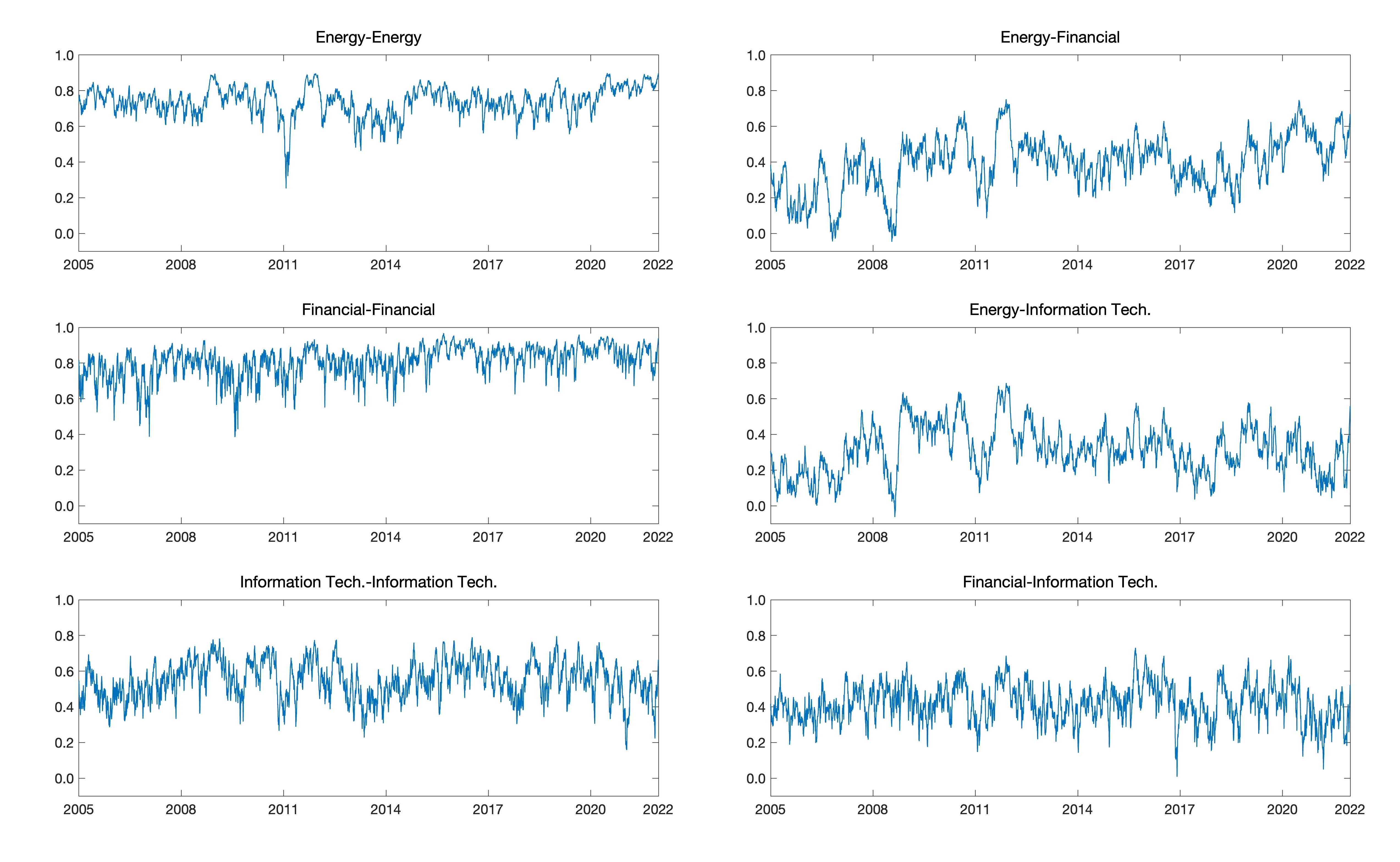
Figure 2: Within-sector and between-sector conditional correlations implied by the estimated Score-Driven model with a sector-based cluster structure in correlations and the Convolution-$t$ distribution (Cluster-$t$ with block correlation matrix).

6.2 Large Universe: Dynamic Correlation Matrix for $100$ Assets

Next, we estimate the model with the large universe, where $C_{t}$ has dimension $100\times 100$. We use the sector classification, see Table 1, to define the block structure on $C_{t}$. Ten (of the eleven) sectors represented in the Large Universe, such that $K=10$, and the number of unique correlations in $C_{t}$ is reduced from 4,950 to 55. We estimate the score-driven model with and without correlation targeting, see Section 5.2. With correlation targeting, the intercept, $\mu$, is estimated first, and the remaining parameters are estimated in a second stage.

Table 5: Large Universe Estimation Results: $C_{t}$ with Block Structure

			Score-Block Model with Full Parametrization										Score-Block Model with Correlation Targeting
			Gaussian		Multiv.-$t$		Canon-$t$		Cluster-$t$		Hetero-$t$		Gaussian		Multiv.-$t$		Canon-$t$		Cluster-$t$		Hetero-$t$
$\mu$	Mean		0.053		0.051		0.056		0.056		0.055		0.053		0.053		0.053		0.053		0.053
	Min		0.004		0.001		0.008		0.008		0.007		0.002		0.002		0.002		0.002		0.002
	$Q_{25}$		0.026		0.025		0.026		0.027		0.026		0.025		0.025		0.025		0.025		0.025
	$Q_{50}$		0.038		0.037		0.038		0.039		0.040		0.036		0.036		0.036		0.036		0.036
	$Q_{75}$		0.048		0.049		0.048		0.048		0.050		0.049		0.049		0.049		0.049		0.049
	Max		0.333		0.327		0.343		0.348		0.342		0.349		0.349		0.349		0.349		0.349
$\beta$	Mean		0.842		0.886		0.888		0.903		0.887		0.850		0.891		0.902		0.915		0.905
	Min		0.443		0.432		0.612		0.654		0.619		0.401		0.415		0.614		0.651		0.621
	$Q_{25}$		0.794		0.859		0.817		0.853		0.808		0.799		0.854		0.827		0.861		0.846
	$Q_{50}$		0.897		0.983		0.935		0.940		0.944		0.898		0.983		0.941		0.951		0.954
	$Q_{75}$		0.975		0.996		0.989		0.985		0.989		0.976		0.996		0.991		0.989		0.990
	Max		0.999		0.999		0.999		0.999		0.999		0.999		1.000		0.999		0.999		0.999
$\alpha$	Mean		0.030		0.023		0.042		0.041		0.041		0.030		0.023		0.041		0.039		0.041
	Min		0.001		0.003		0.005		0.006		0.004		0.001		0.004		0.008		0.005		0.003
	$Q_{25}$		0.013		0.007		0.015		0.014		0.016		0.013		0.007		0.013		0.015		0.015
	$Q_{50}$		0.028		0.015		0.035		0.038		0.036		0.028		0.015		0.032		0.029		0.036
	$Q_{75}$		0.045		0.029		0.057		0.058		0.055		0.045		0.028		0.058		0.055		0.055
	Max		0.102		0.108		0.137		0.127		0.140		0.103		0.106		0.138		0.128		0.139
$\nu_{0}$					10.06		12.25								10.11		12.20
$\nu_{1}$							7.111		7.320		4.852†						7.158		7.341		4.882†
$\nu_{2}$							5.778		6.012		4.723†						5.489		5.812		4.635†
$\nu_{3}$							6.640		6.903		4.451†						6.397		6.644		4.368†
$\nu_{4}$							5.373		5.579		3.884†						5.306		5.546		3.849†
$\nu_{5}$							5.657		5.896		4.049†						5.627		5.847		4.018†
$\nu_{6}$							6.024		6.263		4.070†						5.983		6.183		4.021†
$\nu_{7}$							6.018		6.159		4.280†						6.008		6.127		4.289†
$\nu_{8}$							5.581		5.784		3.829†						5.516		5.706		3.779†
$\nu_{9}$							7.022		7.286		5.347†						7.043		7.283		5.337†
$\nu_{10}$							5.693		6.007		4.366†						5.658		5.945		4.334†
$p$			165		166		176		175		265		110		111		121		120		210
$\ell$			-481966		-464247		-448572		-446633		-436613		-482019		-464307		-448640		-446711		-436704
$\ell_{m}$			-607256		-588971		-589777		-587713		-586615		-607256		-589006		-589625		-587506		-586446
$\ell_{c}$			125292		124724		141204		141079		150002		125236		124699		140986		140795		149742
AIC			964262		928826		897496		893616		873756		964258		928836		897522		893662		873828
BIC			965312		929882		898616		894729		875442		964958		929542		898292		894425		875164

Note: Parameter estimates for the full sample period, January 2005 to December 2021. Score-Driven models with a block correlation structure and five distributional specifications are estimated without correlation targeting (left panel) and with correlation targeting (right panel). We report summary statistics for the estimates of $\mu$, $\alpha$, and $\beta$, and all estimates of the degrees of freedom, except for the Heterogeneous Convolution-$t$ specifications where we report the average estimate within each cluster., as identified with the $\dagger$-superscript. $p$ is the number of parameters and we report the maximized log-likelihoods, $\ell=\ell_{m}+\ell_{c}$, and its two components: the log-likelihoods for the nine marginal distributions, $\ell_{m}$, and the corresponding log-copula density, $\ell_{c}$. We also report the AIC $=-2\ell+2p$ and BIC $=-2\ell+p\ln T$. Bold font is used to identify the “best performing” specification in each row for models with and without correlation targeting.

Table 5 reports the estimation results for the the score-driven models with block correlation matrices. The left panel has estimation results for models without correlation targeting, and the right panel has the estimation results based on correlation targeting. The estimates identified with a $\dagger$-superscript, are the average degrees of freedom within each cluster. These are used for specifications with heterogeneous Convolution-$t$ specifications (Hetero-$t$), which estimates 100 degrees of freedom parameters. Compared with the results for the Small Universe, we note some interesting difference. First, different from the results on small universe, the model with hetero-$t$ distribution now provides the best fitting performance, and compared with Cluster-$t$ distribution, its improvement concentrates on the copula part. This may due to the high level of heterogeneity across the large dataset, and the simple classification based GICS is poor. Second, the models estimated with targeting perform well and have the smallest BIC across all distributional specifications.

6.3 Out-of-sample Results

We next compare the out-of-sample (OOS) performance of the different models/specifications. We estimate all models (once) using data from 2005-2014 and evaluate the estimated models with (out-of-sample) data that spans the years: 2015-2021.

The OOS results for the Small Universe are shown in Panel A of Table 6. We decompose the predicted log-likelihood, $\ell$, into the marginal, $\ell_{m}$, and copula, $\ell_{c}$, components. For each of the five distributional specifications, we have highlighted the largest predicted log-likelihood, which is the Score-Driven model without a block structure on $C_{t}$, for all five distributions. This is consistent with our in-sample results, where this model also had the largest (in-sample) log-likelihood for each of the five distributional specifications, see Tables 3 and 4. Overall, the Convolution-$t$ distribution with a sector-based cluster structure, Cluster-$t$, has the largest predictive log-likelihood. We also note that the DCC model is has the worst performance across all distributional specifications. In sample, the DCC model was slightly better than the Score-Driven model with a block correlation matrix, for two of the five distributions (Gaussian and multivariate $t$). This suggests that the DCC suffer from an overfitting problem.

Table 6: Out-of-sample Results

Panel A: Out-of-sample Results for 9 Assets
	Gaussian		Multiv.-$t$		Canon-$t$		Cluster-$t$		Hetero-$t$
DCC Model
$p$	126		127		130		129		135
$\ell$	-17148		-15887		-15719		-15538		-15648
$\ell_{m}$	-22721		-21825		-21849		-21770		-21784
$\ell_{c}$	5573		5938		6130		6232		6136
Score-Full Model
$p$	108		109		112		111		117
$\ell$	-17139		-15812		-15672		-15459		-15572
$\ell_{m}$	-22721		-21839		-21864		-21782		-21804
$\ell_{c}$	5582		6027		6192		6323		6232
Score-Block Model
$p$	18		19		22		21		27
$\ell$	-17142		-15832		-15698		-15484		-15591
$\ell_{m}$	-22721		-21842		-21865		-21783		-21805
$\ell_{c}$	5579		6010		6167		6299		6214
Panel B: Out-of-sample Results for 100 Assets
	Gaussian		Student-$t$		Convo-$t$		Group-$t$		Hetero-$t$
Score-Block Model
$p$	165		166		176		175		265
$\ell$	-202633		-192366		-184318		-183362		-179509
$\ell_{m}$	-251946		-242925		-243415		-242198		-241225
$\ell_{c}$	49313		50559		59098		58836		61716
Score-Block Model with Correlation Targeting
$p$	110		111		121		120		210
$\ell$	-201910		-192041		-184080		-183145		-179205
$\ell_{m}$	-251946		-242891		-243364		-242005		-241072
$\ell_{c}$	50036		50850		59284		58860		61867

Note: Out-of-sample results for the sample period (January 2015 to December 2021). $p$ is the number of parameters, $\ell$ is the log-likelihood function. The Akaike and Bayesian information criteria are respectively computed as AIC $=-2\ell+2p$, and BIC $=-2\ell+p\ln T$. We include the Score-driven log Group-correlation model with several distribution assumptions. The highest log-likelihood and smallest AIC and BIC in each row are highlighted in bold.

We report the OOS results for the Large Universe in Panel B of Table 6, where all model-specifications employ a block structure on $C_{t}$. The empirical results favor correlation targeting, because the Score-Driven model with correlation targeting has the largest predicted log-likelihood for each of the five distributions. Across the five distributions, the Convolution-$t$ distribution based on $100$, independent $t$-distributions, Hetero-$t$, has the largest predictive log-likelihood.

7 Summary

We have introduced the Cluster GARCH model, which is a novel multivariate GARCH model, with two types of cluster structures. One that relates to the correlation structure and one that define non-linear dependencies. The Cluster GARCH framework combines several useful components from the existing literature. For instance, we incorporate the block correlation structure by Engle and Kelly, (2012), the correlation parametrization by Archakov and Hansen, (2021), and the convolution-$t$ distributions by Hansen and Tong, (2024). A convolution-$t$ distribution is a multivariate heavy-tailed distribution with cluster structures, flexible nonlinear dependencies, and heterogeneous marginal distributions. We also adopted the score-driven framework by Creal et al., (2013) to model the dynamic variation in the correlation structure. The convolution-$t$ distributions are well-suited for score-driven models, because their density functions are sufficiently tractable, allowing us to derive closed-form expressions for the key ingredients in score-driven models: the score and the Hessian. We derived detailed results for three special types of convolution-$t$ distributions. These are labelled Canonical-Block-$t$, Cluster-$t$, and Hetero-$t$, and their score functions and Fisher informations are all available in closed-form.

Applying the model to high-dimensional systems is possible when the block correlation structure is imposed. This was pointed out in Archakov et al., (2020), but the present paper is first to demonstrate this empirically with $n=100$. This was achieved with $K=10$ sector-based clusters that was used to define the block structure on the correlation matrix. The block structure is advantages for several reason. First, it reduces the number of distinct correlations in $C_{t}$ from 4,950 to 55 ($n(n-1)/2$ to $K(K+1)/2$). Second, many likelihood computations are greatly simplified due to the canonical representation of block correlation matrix, see Archakov and Hansen, (2024). An important implication for the dynamic model is that computations only involve inverses, determinants, square-roots of $K\times K$ matrices rather than $n\times n$ matrices.

We conduct an extensive empirical investigation on the performance of our dynamic model for correlation matrices. And we consider a “small universe” with $n=9$ assets and a “large universe” with $n=100$ assets. The empirical results find strong support for convolution-$t$ distributions that outperforms conventional distributions, in-sample as well as out-of-sample. Moreover, the score-driven framework out-performs the standard DCC model in all cases (dimensions and choice of distribution). The score-driven model with a sector-based block correlation matrix has the smallest BIC.

Appendix A Proofs

Proof of Proposition 1. Let $X\sim t_{\nu}^{\mathrm{std}}(0,I_{n})$ and consider $X_{\alpha}\equiv\alpha^{\prime}X$, for some $\alpha\in\mathbb{R}^{n}$. It follows that $X_{\alpha}=aY$ where $a=\left\|\alpha\right\|=\sqrt{\alpha^{\prime}\alpha}$ and $Y$ is a univariate random variable with distribution, $Y\sim t_{\nu}^{\mathrm{std}}(0,1)$. The characteristics function for the conventional Student’s $t$-distribution with $\nu$ degrees of freedom, see Hurst, (1995) and Joarder, (1995), is given by:

$$\varphi_{\nu}(s)=\frac{K_{\frac{\nu}{2}}(\sqrt{\nu}|s|)(\sqrt{\nu}|s|)^{\frac{1}{2}\nu}}{\Gamma\left(\frac{\nu}{2}\right)2^{\frac{\nu}{2}-1}},$$

where $K_{\frac{\nu}{2}}(\cdot)$ is the modified Bessel function of the second kind, such that the characteristic function for $Y$ is given by,

$$\varphi_{\nu}^{\mathrm{std}}(s)=\varphi_{\nu}(\sqrt{\tfrac{\nu-2}{\nu}}s)=\frac{K_{\frac{\nu}{2}}(\sqrt{\nu-2}|s|)(\sqrt{\nu-2}|s|)^{\frac{1}{2}\nu}}{\Gamma\left(\frac{\nu}{2}\right)2^{\frac{\nu}{2}-1}},$$

and the characteristic function for $X_{\alpha}$ is simply $\varphi_{X_{\alpha}}(s)=\varphi_{\nu}^{\mathrm{std}}(s\left\|\alpha\right\|)$.

Next, the $j$-th element of $Z=C^{\frac{1}{2}}U$ can be expresses as

$$Z_{j}=e_{j,n}^{\prime}C^{\frac{1}{2}}U=\sum_{g=1}^{G}\left(e_{j,n}^{\prime}C^{\frac{1}{2}}P_{g}\right)V_{g}=\sum_{g=1}^{G}\alpha_{jg}^{\prime}V_{g},$$

where $\alpha_{jg}=P_{g}^{\prime}C^{\frac{1}{2}}e_{j,n}\in\mathbb{R}^{m_{g}}$ and $e_{j,n}$ is the $j$-th column of identity matrix $I_{n}$. From the independence of $V_{1},\ldots,V_{G}$ it now follows that the characteristic function for $Z_{j}$ is given by

$$\varphi_{Z_{j}}(s) =\prod_{g=1}^{G}\mathbb{E}\left(\exp\left(is\alpha_{jg}^{\prime}V_{g}\right)\right)=\prod_{g=1}^{G}\varphi_{\nu}^{\mathrm{std}}\left(s\|\alpha_{jg}\|\right).$$

Finally, from the inverse Fourier transform, we can recover the probability and cumulative density functions from the characteristic functions of $Z_{j}$, given by

$$f_{Z_{j}}(z)=\frac{1}{\pi}\int_{0}^{\infty}{\rm Re}\left[e^{-isz}\varphi_{Z_{j}}(s)\right]\mathrm{d}s,$$

and

$$F_{Z_{j}}(z)=\frac{1}{2}-\frac{1}{\pi}\int_{0}^{\infty}\frac{{\rm Im}\left[e^{-isz}\varphi_{Z_{j}}(s)\right]}{s}\mathrm{d}s,$$

respectively. $\square$

A.1 Proofs of Results for Score Model (Section 4)

First some notation. Let $A$ and $B$ be $k\times k$ matrices, then $A\otimes B$ denotes the Kronecker product. We use $A_{\otimes}$ to denote $A\otimes A$ and $A\oplus B$ for $A\otimes B+B\otimes A$ as in Creal et al., (2012). The ${\rm vec}(A)$ stacks the columns of matrix $A$ into a $k^{2}\times 1$ column vector, while ${\rm vech}(A)$ stacks the lower triangular part (including diagonal elements) into a $k^{*}\times 1$ column vector, where $k^{*}=k(k+1)/2$. The $k\times k$ identity matrix is denoted by $I_{k}$.

From the eigendecomposition, $C=Q\Lambda Q^{\prime}$, we have from Laub, (2004, Theorem 13.16) that $C\oplus I=(Q\otimes Q)(\Lambda\oplus I)(Q^{\prime}\otimes Q^{\prime}).$ The inverse is therefore given by

$$\left(C\oplus I\right)^{-1}=\left(Q\otimes Q\right)\left(\Lambda^{-1}\oplus I\right)\left(Q^{\prime}\otimes Q^{\prime}\right).$$

From Linton and McCrorie, (1995), the expression for $\Gamma=\partial{\rm vec}\left(C\right)/\partial{\rm vec}\left(\log C\right)^{\prime}$ is

$$\Gamma=(Q\otimes Q)\varXi(Q\otimes Q)^{\prime},$$ (A.1)

where $Q$ is an orthonormal matrix from the eigenvectors of $\log A$ with eigenvalues, $\lambda_{1},\ldots,\lambda_{n}$, and $\varXi$ is a $n^{2}\times n^{2}$ diagonal matrix with elements $\delta_{ij}$, for $i,j=1,\ldots,n$

$$\delta_{ij}=\varXi_{(i-1)n+j,(i-1)n+j}=\begin{cases}e^{\lambda_{i}},&\text{ if }\lambda_{i}=\lambda_{j},\\ \frac{e^{\lambda_{i}}-e^{\lambda_{j}}}{\lambda_{i}-\lambda_{j}},&\text{ if }\lambda_{i}\neq\lambda_{j},\end{cases}$$

Note that the the expression for $\partial{\rm vec}\left(\log C\right)/\partial{\rm vec}\left(C\right)^{\prime}$ is just the inverse of $\Gamma$, given by

$$\Gamma^{-1}=(Q\otimes Q)\varXi^{-1}(Q\otimes Q)^{\prime},$$ (A.2)

where $\varXi^{-1}$ is a $n^{2}\times n^{2}$ diagonal matrix with elements $\delta_{ij}^{-1}$, for $i,j=1,\ldots,n$.

Next, we presents expectations of some quantities involving the $t_{\nu}^{\mathrm{std}}(0,I_{n})$ distribution, involving the following constant,

$$\zeta_{p,q}=\left(\tfrac{\nu+n}{\nu-2}\right)^{\frac{p}{2}}\left(\tfrac{\nu-2}{2}\right)^{\frac{q}{2}}\frac{\Gamma(\frac{\nu+n}{2})}{\Gamma(\tfrac{\nu}{2})}\frac{\Gamma(\tfrac{\nu+p-q}{2})}{\Gamma(\tfrac{\nu+p+n}{2})}.$$

Lemma A.1.

Suppose that $X\sim t_{\nu}^{\mathrm{std}}(0,I_{n})$ and define

$$W=\frac{\nu+n}{\nu-2+X^{\prime}X}.$$

(i) For any integrable function $g$ and any $p>2-\nu$, it holds that

$$\mathbb{E}\left[W^{\frac{p}{2}}g(X)\right]=\zeta_{p,0}\mathbb{E}\left[g(Y)\right],$$

where $Y\sim t_{\nu+p}^{\mathrm{std}}\left(0,\frac{v-2}{v+p-2}I_{n}\right)$.

(ii) Moreover, if $g$ is homogeneous of degree $q<\nu+p$, then

$$\mathbb{E}\left[W^{\frac{p}{2}}g(X)\right]=\zeta_{p,q}\mathbb{E}\left[g(Z)\right],$$

where $Z\sim N\left(0,I_{n}\right)$.

By integrable function, $g$, the requirement is $\mathbb{E}|g(Y)|<\infty$ and $\mathbb{E}|g(Z)|<\infty$ in parts (i) and (ii), respectively. Note that $p$ is allowed to be negative, since $2-\nu<0$. Also, if $p/2$ is a positive integer, then

$$\zeta_{p,q} = \left(\tfrac{\nu+n}{\nu-2}\right)^{\frac{p}{2}}\left(\tfrac{\nu-2}{2}\right)^{\frac{q}{2}}\frac{\tfrac{\nu+q}{2}}{\tfrac{\nu+n}{2}}\frac{\tfrac{\nu+q}{2}+1}{\tfrac{\nu+n}{2}+1}\cdots\frac{\tfrac{\nu+q}{2}+\tfrac{p}{2}-1}{\tfrac{\nu+n}{2}+\tfrac{p}{2}-1}$$

$$= \left(\tfrac{\nu+n}{\nu-2}\right)^{\frac{p}{2}}\left(\tfrac{\nu-2}{2}\right)^{\frac{q}{2}}\frac{\nu+q}{\nu+n}\frac{\nu+q+2}{\nu+n+2}\cdots\frac{\nu+q+p-2}{\nu+n+p-2}$$

$$= \left(\tfrac{\nu+n}{\nu-2}\right)^{\frac{p}{2}}\left(\tfrac{\nu-2}{2}\right)^{\frac{q}{2}}\prod_{k=0}^{\tfrac{p}{2}-1}\frac{\nu+q+2k}{\nu+n+2k}.$$

where we used $\Gamma(x+1)=x\Gamma(x)$, repeatedly. This simplifies the terms we use to derive the Fisher information matrix in several score models

$$\begin{array}[]{rclcrcl}\zeta_{2,0}&=&\frac{\nu}{\nu-2},&&\zeta_{2,2}&=&1,\\ \zeta_{4,0}&=&\frac{(\nu+n)}{(\nu+n+2)}\frac{(\nu+2)\nu}{(\nu-2)^{2}},&&\zeta_{4,2}&=&\frac{(\nu+n)\nu}{(\nu+n+2)(\nu-2)},\\ &&&&\zeta_{4,4}&=&\frac{(\nu+n)}{(\nu+n+2)}.\end{array}$$

Proof of Lemma A.1. Let $\kappa_{\nu,n}=\Gamma(\tfrac{\nu+n}{2})/\Gamma(\tfrac{\nu}{2})$ and the density for $X\sim t_{\nu}^{\mathrm{std}}(0,I_{n})$ is

$$f_{x}(x)=\kappa_{\nu,n}[(\nu-2)\pi]^{-\frac{n}{2}}\left(1+\tfrac{x^{\prime}x}{\nu-2}\right)^{-\frac{\nu+n}{2}},$$

whereas the density for $Y\sim t_{\nu+p}^{\mathrm{std}}(0,\frac{v-2}{v+p-2}I_{n})$ is

$$f_{y}(y) = \kappa_{\nu+p,n}[(\nu+p-2)\pi]^{-\frac{n}{2}}\left(\tfrac{\nu+p-2}{\nu-2}\right)^{\frac{n}{2}}\left(1+\tfrac{1}{\nu+p-2}x^{\prime}\left[\tfrac{\nu-2}{\nu+p-2}I_{n}\right]^{-1}x\right)^{-\frac{\nu+p+n}{2}}$$

$$= \kappa_{\nu+p,n}[(\nu-2)\pi]^{-\frac{n}{2}}\left(1+\tfrac{x^{\prime}x}{\nu-2}\right)^{-\frac{\nu+p+n}{2}}.$$

The expected value we seek is

$$\mathbb{E}\left[W^{\frac{p}{2}}g(X)\right] = \int\left(\tfrac{\nu+n}{\nu-2+x^{\prime}x}\right)^{\frac{p}{2}}g(x)\kappa_{\nu,n}[(\nu-2)\pi]^{-\frac{n}{2}}\left(1+\tfrac{x^{\prime}x}{\nu-2}\right)^{-\frac{\nu+n}{2}}\mathrm{d}x$$

$$= \left(\tfrac{\nu+n}{\nu-2}\right)^{\frac{p}{2}}\int g(x)\kappa_{\nu,n}[(\nu-2)\pi]^{-\frac{n}{2}}\left(1+\tfrac{x^{\prime}x}{\nu-2}\right)^{-\frac{\nu+p+n}{2}}\mathrm{d}x$$

$$= \left(\tfrac{\nu+n}{\nu-2}\right)^{\frac{p}{2}}\frac{\kappa_{\nu,n}}{\kappa_{\nu+p,n}}\int g(x)f_{y}(x)\mathrm{d}x,$$

and the results for part (i) follows, since

$$\zeta_{p,0}=\left(\tfrac{\nu+n}{\nu-2}\right)^{\frac{p}{2}}\frac{\Gamma(\tfrac{\nu+n}{2})/\Gamma(\tfrac{\nu}{2})}{\Gamma(\tfrac{\nu+p+n}{2})/\Gamma(\tfrac{\nu+p}{2})}=\left(\tfrac{\nu+n}{\nu-2}\right)^{\frac{p}{2}}\frac{\kappa_{\nu,n}}{\kappa_{\nu+p,n}}.$$

To prove (ii) we use that $Y\sim t_{\nu+p}^{\mathrm{std}}\left(0,\frac{v-2}{v+p-2}I_{n}\right)$ can be expressed as $Y=Z/\sqrt{\xi/(\nu-2)}$ where $Z\sim N(0,I_{n})$ and $\xi$ is an independent $\chi^{2}$-distributed random variable with $\nu+p$ degrees of freedom. Hence, $Y=\psi Z$, with $\psi=1/\sqrt{\xi/(\nu-2)}$, such that $\psi^{q}=\left(\tfrac{\nu-2}{\xi}\right)^{\frac{q}{2}}.$ Now using part (i) and that $g$ is homogeneous, we find

$$\mathbb{E}\left[W^{\frac{p}{2}}g(X)\right] = \zeta_{p,0}\mathbb{E}\left[g(Y)\right]=\zeta_{p,0}\mathbb{E}\left[\psi^{q}g(Z)\right]$$

$$= \zeta_{p,0}\left(\nu-2\right)^{\frac{q}{2}}\mathbb{E}[\xi^{-\frac{q}{2}}]\mathbb{E}\left[g(Z)\right],$$

$$= \zeta_{p,0}\left(\nu-2\right)^{\frac{q}{2}}\frac{\Gamma(\tfrac{\nu+p-q}{2})}{\Gamma(\tfrac{\nu+p}{2})}\left(\tfrac{1}{2}\right)^{\frac{q}{2}}\mathbb{E}\left[g(Z)\right]$$

$$= \left(\tfrac{\nu+n}{\nu-2}\right)^{\frac{p}{2}}\frac{\Gamma(\tfrac{\nu+n}{2})}{\Gamma(\tfrac{\nu}{2})}\frac{\Gamma(\tfrac{\nu+p-q}{2})}{\Gamma(\tfrac{\nu+p+n}{2})}\left(\tfrac{\nu-2}{2}\right)^{\frac{q}{2}}\mathbb{E}\left[g(Z)\right],$$

where we used that $\xi$ and $Z$ are independent, and Creal et al., (2012, Results 2), which states that if $\xi\sim\chi_{\nu+p}^{2}$, then

$$\mathbb{E}\left(\xi^{-\frac{q}{2}}\right)=\frac{\Gamma(\tfrac{\nu+p-q}{2})}{\Gamma(\tfrac{\nu+p}{2})}\left(\tfrac{1}{2}\right)^{\frac{q}{2}},\qquad\text{for}\quad q<\nu+p.$$

This completes the proof. $\square$

Proof of Theorem 1. The log-likelihood function for a vector, $Z$, with the multivariate $t$-distribution, is given by

$$\ell(Z) =c_{\nu,n}-\tfrac{1}{2}\log\left|C\right|-\tfrac{\nu+n}{2}\log\left(1+\tfrac{1}{\nu-2}Z^{\prime}C^{-1}Z\right).$$

So, we define $W=\left(\nu+n\right)/\left(\nu-2+Z^{\prime}C^{-1}Z\right)$, we have

$$\frac{\partial\ell}{\partial{\rm vec}(C)^{\prime}} =-\tfrac{1}{2}{\rm vec}\left(C^{-1}\right)^{\prime}-\tfrac{1}{2}\frac{\nu+n}{\nu-2+Z^{\prime}C^{-1}Z}\frac{\partial\left(Z^{\prime}C^{-1}Z\right)}{\partial{\rm vec}(C^{-1})^{\prime}}\frac{\partial{\rm vec}(C^{-1})}{\partial{\rm vec}(C)^{\prime}}$$

$$=-\tfrac{1}{2}\left[{\rm vec}\left(C^{-1}\right)^{\prime}+W{\rm vec}\left(ZZ^{\prime}\right)^{\prime}C_{\otimes}^{-1}\right]$$

$$=\tfrac{1}{2}\left[W{\rm vec}\left(ZZ^{\prime}\right)^{\prime}-{\rm vec}\left(C\right)^{\prime}\right]C_{\otimes}^{-1},$$

such that the score is given by

$$\nabla^{\prime}=\frac{\partial\ell}{\partial\gamma^{\prime}}=\frac{\partial\ell}{\partial{\rm vec}(C)^{\prime}}\frac{\partial{\rm vec}(C)^{\prime}}{\partial\gamma^{\prime}}=\tfrac{1}{2}\left[W{\rm vec}\left(ZZ^{\prime}\right)^{\prime}-{\rm vec}\left(C\right)^{\prime}\right]C_{\otimes}^{-1}M.$$

From Archakov and Hansen, (2021, Proposition 3) we have the expression

$$M=\frac{\partial{\rm vec}\left(C\right)}{\partial\gamma^{\prime}}=\left(E_{l}+E_{u}\right)^{\prime}E_{l}\left(I-\Gamma E_{d}^{\prime}\left(E_{d}\Gamma E_{d}^{\prime}\right)^{-1}E_{d}\right)\Gamma\left(E_{l}+E_{u}\right)^{\prime},$$ (A.3)

which uses the fact that $\partial{\rm vec}\left(C\right)/\partial{\rm vecl}\left(C\right)=E_{l}+E_{u}$, where $E_{l}$, $E_{u}$, $E_{d}$ are elimination matrices, and the expression $\Gamma=\partial{\rm vec}\left(C\right)/\partial{\rm vec}\left(\log C\right)^{\prime}$ is given in (A.1).

Next we rewrite $\nabla$ as

$$\nabla^{\prime} =\tfrac{1}{2}\left[W{\rm vec}\left(ZZ^{\prime}\right)^{\prime}-{\rm vec}\left(C\right)^{\prime}\right]C_{\otimes}^{-1}M=\tfrac{1}{2}\left[W{\rm vec}\left(UU^{\prime}\right)^{\prime}-{\rm vec}\left(I\right)^{\prime}\right]C_{\otimes}^{-\tfrac{1}{2}}M,$$

where $U=C^{-\frac{1}{2}}Z\sim t_{\nu}^{\mathrm{std}}\left(0,I_{n}\right)$, such that

$$\mathcal{I}=\mathbb{E}\left[\nabla\nabla^{\prime}\right]=\frac{1}{4}M^{\prime}C_{\otimes}^{-\tfrac{1}{2}}\left[\mathbb{E}\left(W^{2}{\rm vec}\left(UU^{\prime}\right){\rm vec}\left(UU^{\prime}\right)^{\prime}\right)-{\rm vec}\left(I\right){\rm vec}\left(I\right)^{\prime}\right]C_{\otimes}^{-\tfrac{1}{2}}M.$$

From Lemma A.1 with $\phi=\zeta_{42}=(v+n)/(v+n+2)$, we have

$$\mathbb{E}\left[W^{2}{\rm vec}\left(UU^{\prime}\right){\rm vec}\left(UU^{\prime}\right)^{\prime}\right]=\phi\mathbb{E}\left[{\rm vec}\left(\tilde{Z}\tilde{Z}^{\prime}\right){\rm vec}\left(\tilde{Z}\tilde{Z}^{\prime}\right)^{\prime}\right]=\phi\left[H_{n}+{\rm vec}\left(I\right){\rm vec}\left(I\right)^{\prime}\right],$$

where $\tilde{Z}\sim N\left(0,I_{n}\right)$. The expression for last expectation follows from Magnus and Neudecker, (1979, Theorem 4.1), which states that

$$\mathbb{E}\left[{\rm vec}\left(\tilde{Z}\tilde{Z}^{\prime}\right){\rm vec}\left(\tilde{Z}\tilde{Z}^{\prime}\right)^{\prime}\right]=H_{n}+{\rm vec}\left(I\right){\rm vec}\left(I\right)^{\prime},$$

if $\tilde{Z}\sim N\left(0,I_{n}\right)$, where $H_{n}=I_{n^{2}}+K_{n}$, and $K_{n}$ is the commutation matrix. Finally,

$$\mathcal{I} =\tfrac{1}{4}M^{\prime}C_{\otimes}^{-\tfrac{1}{2}}\left[\phi H_{n}+\left(\phi-1\right){\rm vec}\left(I_{n}\right){\rm vec}\left(I_{n}\right)^{\prime}\right]C_{\otimes}^{-\tfrac{1}{2}}M$$

$$=\tfrac{1}{4}M^{\prime}\left[\phi C_{\otimes}^{-1}H_{n}+(\phi-1){\rm vec}\left(C^{-1}\right){\rm vec}\left(C^{-1}\right)^{\prime}\right]M.$$ (A.4)

This completes the proof. $\square$

Proof of Theorem 1. For this case we have the log-likelihood function

$$\ell\left(Z\right) =-\log|C^{\frac{1}{2}}|+\sum_{g=1}^{G}c_{g}-\tfrac{\nu_{g}+m_{g}}{2}\log\left(1+\tfrac{1}{\nu_{g}-2}V_{g}^{\prime}V_{g}\right),$$

where $V_{g}=P_{g}^{\prime}U=P_{g}^{\prime}C^{-\frac{1}{2}}Z$, and $J_{g}=P_{g}P_{g}^{\prime}$. Because we have

$$\frac{\partial\left(V_{g}^{\prime}V_{g}\right)}{\partial{\rm vec}(C^{\frac{1}{2}})^{\prime}} =\frac{\partial\left(V_{g}^{\prime}V_{g}\right)}{\partial V_{g}^{\prime}}\frac{\partial{\rm vec}(P_{g}^{\prime}C^{-\frac{1}{2}}Z)}{\partial{\rm vec}(C^{-\frac{1}{2}})^{\prime}}\frac{\partial{\rm vec}(C^{-\frac{1}{2}})}{\partial{\rm vec}(C^{\frac{1}{2}})^{\prime}}$$

$$=-2V_{g}^{\prime}\left(Z^{\prime}\otimes P_{g}^{\prime}\right)C_{\otimes}^{-\frac{1}{2}}$$

$$=-2V_{g}^{\prime}\left(U^{\prime}\otimes P_{g}^{\prime}C^{-\frac{1}{2}}\right)$$

$$=-2{\rm vec}\left(C^{-\frac{1}{2}}P_{g}V_{g}U^{\prime}\right)^{\prime}.$$

Define $W_{g}=\left(\nu_{g}+m_{g}\right)/\left(\nu_{g}-2+V_{g}^{\prime}V_{g}\right)$, then we have

$$\frac{\partial\ell}{\partial{\rm vec}(C^{\frac{1}{2}})} =\sum_{g=1}^{G}W_{g}{\rm vec}\left(C^{-\frac{1}{2}}P_{g}V_{g}U^{\prime}\right)-{\rm vec}\left(C^{-\frac{1}{2}}\right)=\left(I_{n}\otimes C^{-\frac{1}{2}}\right)\nabla_{s},$$

where $\nabla_{s}=\sum_{g=1}^{G}W_{g}{\rm vec}\left(P_{g}V_{g}U^{\prime}\right)-{\rm vec}\left(I_{n}\right)$. So, we have the formula for the score

$$\nabla^{\prime} =\frac{\partial\ell}{\partial\gamma^{\prime}}=\frac{\partial\ell}{\partial{\rm vec}(C^{\frac{1}{2}})}\frac{\partial{\rm vec}(C^{\frac{1}{2}})}{\partial{\rm vec}(C)^{\prime}}\frac{\partial{\rm vec}(C)}{\partial\gamma^{\prime}}=\nabla_{s}^{\prime}\Omega M$$

where the matrix $M$ is defined in (A.3) and $\Omega=(I_{n}\otimes C^{-\frac{1}{2}})(C^{\frac{1}{2}}\oplus I_{n})^{-1}$, which is based on

$$\frac{\partial{\rm vec}(C^{\frac{1}{2}})}{\partial{\rm vec}(C)^{\prime}}=\left(\frac{\partial{\rm vec}(C)}{\partial{\rm vec}(C^{\frac{1}{2}})^{\prime}}\right)^{-1}=\left(C^{\frac{1}{2}}\oplus I_{n}\right)^{-1}.$$

This proves (20). Next, the inverse of the $n^{2}\times n^{2}$ matrix $C^{\frac{1}{2}}\oplus I$ is available in closed form, see Appendix A, based on the eigendecomposition $C^{\frac{1}{2}}=Q\Lambda^{\frac{1}{2}}Q^{\prime}$. This does not add to the computation burden additionally, because the eigendecomposition of $C^{\frac{1}{2}}$ is available from that of $\log C=Q\log\Lambda Q^{\prime}$, which was needed for computing $\Theta$ from $M$.

The Information Matrix

Next we turn to the information matrix. Note that$\mathcal{I}=M^{\prime}\Omega\mathbb{E}\left(\nabla_{s}\nabla_{s}^{\prime}\right)\Omega M$, with $\mathbb{E}\left(\nabla_{s}\nabla_{s}^{\prime}\right)$ given by

$$\mathbb{E}\left(\nabla_{s}\nabla_{s}^{\prime}\right) =\mathbb{E}\left[\sum_{k=1}^{G}\sum_{l=1}^{G}W_{k}W_{l}{\rm vec}\left(P_{k}V_{k}U^{\prime}\right){\rm vec}\left(P_{l}V_{l}U^{\prime}\right)^{\prime}-{\rm vec}\left(I_{n}\right){\rm vec}\left(I_{n}\right)^{\prime}\right]$$

For later use, we define $\psi_{k}=\zeta_{42}$, and $\phi_{k}=\zeta_{44}$, for $k=1,\ldots,G$, where the constants are given from Lemma A.1, given by

$$\phi_{k}=\frac{\nu_{k}+m_{k}}{\nu_{k}+m_{k}+2},\quad\text{and}\quad\psi_{k}=\phi_{k}\frac{\nu_{k}}{\nu_{k}-2},$$

and define the function $\varphi\left(k,l\right)$ as

$$\varphi\left(k,l\right)=W_{k}W_{l}{\rm vec}\left(P_{k}V_{k}U^{\prime}\right){\rm vec}\left(P_{l}V_{l}U^{\prime}\right)^{\prime}.$$

Note that we will use the following preliminary results in later analysis

$$U=\sum_{g=1}^{G}P_{g}V_{g},\quad J_{g}=P_{g}P_{g}^{\prime},\quad\sum_{g=1}^{G}J_{g}=I_{n}.$$

Expectation of $\varphi\left(k,l\right)$ when $k=l$

We have the expectation for $\varphi\left(k,k\right)$ given by

$$\mathbb{E}\left[\varphi\left(k,k\right)\right]= \mathbb{E}\left[W_{k}^{2}\sum_{p=1}^{G}{\rm vec}\left(P_{k}V_{k}V_{p}^{\prime}P_{p}^{\prime}\right)\sum_{q=1}^{G}{\rm vec}\left(P_{k}V_{k}V_{q}^{\prime}P_{q}^{\prime}\right)^{\prime}\right]$$

$$= \mathbb{E}\left[W_{k}^{2}\sum_{p\neq k}^{G}{\rm vec}\left(P_{k}V_{k}V_{p}^{\prime}P_{p}^{\prime}\right){\rm vec}\left(P_{k}V_{k}V_{p}^{\prime}P_{p}^{\prime}\right)^{\prime}+W_{k}^{2}{\rm vec}\left(P_{k}V_{k}V_{k}^{\prime}P_{k}^{\prime}\right){\rm vec}\left(P_{k}V_{k}V_{k}^{\prime}P_{k}^{\prime}\right)^{\prime}\right].$$

Based on Lemma A.1 with $\psi_{k}=\zeta_{42}$, we have

$$\sum_{p\neq k}^{G}\mathbb{E}\left[W_{k}^{2}{\rm vec}\left(P_{k}V_{k}V_{p}^{\prime}P_{p}^{\prime}\right){\rm vec}\left(P_{k}V_{k}V_{p}^{\prime}P_{p}^{\prime}\right)^{\prime}\right]$$

$$= \sum_{p\neq k}^{G}\left(P_{p}\otimes P_{k}\right)\mathbb{E}\left[W_{k}^{2}{\rm vec}\left(V_{k}V_{p}^{\prime}\right){\rm vec}\left(V_{k}V_{p}^{\prime}\right)^{\prime}\right]\left(P_{p}^{\prime}\otimes P_{k}^{\prime}\right)$$

$$= \psi_{k}\sum_{p\neq k}^{G}\left(P_{p}\otimes P_{k}\right)\left(P_{p}^{\prime}\otimes P_{k}^{\prime}\right)$$

$$= \psi_{k}\sum_{p\neq k}^{G}\left(J_{p}\otimes J_{k}\right)$$

$$= \psi_{k}\left(I_{n}-J_{k}\right)\otimes J_{k},$$

and from Lemma A.1 we have $\phi_{k}=\zeta_{44}$, such that

$$\mathbb{E}\left[W_{k}^{2}{\rm vec}\left(P_{k}V_{k}V_{k}^{\prime}P_{k}^{\prime}\right){\rm vec}\left(P_{k}V_{k}V_{k}^{\prime}P_{k}^{\prime}\right)^{\prime}\right]$$

$$= \left(P_{k}\otimes P_{k}\right)\mathbb{E}\left[W_{k}^{2}{\rm vec}\left(V_{k}V_{k}^{\prime}\right){\rm vec}\left(V_{k}V_{k}^{\prime}\right)^{\prime}\right]\left(P_{k}^{\prime}\otimes P_{k}^{\prime}\right)$$

$$= \phi_{k}\left(P_{k}\otimes P_{k}\right)\left[H_{n_{k}}+{\rm vec}(I_{n_{k}}){\rm vec}(I_{n_{k}})^{\prime}\right]\left(P_{k}^{\prime}\otimes P_{k}^{\prime}\right)$$

$$= \phi_{k}\left[J_{k\otimes}H_{n}+{\rm vec}(J_{k}){\rm vec}(J_{k})^{\prime}\right].$$

Finally we arrive at the expression,

$$\mathbb{E}\left[\varphi\left(k,k\right)\right] =\psi_{k}\left(I_{n}-J_{k}\right)\otimes J_{k}+\phi_{k}\left[J_{k\otimes}H_{n}+{\rm vec}(J_{k}){\rm vec}(J_{k})^{\prime}\right].$$

Expectation of $\varphi\left(k,l\right)$ when $k\neq l$

When $k\neq l$, we have

$$\mathbb{E}\left[\varphi\left(k,l\right)\right]= \mathbb{E}\left[W_{k}W_{l}\sum_{p=1}^{G}{\rm vec}\left(P_{k}V_{k}V_{p}^{\prime}P_{p}^{\prime}\right)\sum_{q=1}^{G}{\rm vec}\left(P_{l}V_{l}V_{q}^{\prime}P_{q}^{\prime}\right)^{\prime}\right]$$

$$= \mathbb{E}\left[W_{k}W_{l}{\rm vec}\left(P_{k}V_{k}V_{k}^{\prime}P_{k}^{\prime}\right){\rm vec}\left(P_{l}V_{l}V_{l}^{\prime}P_{l}^{\prime}\right)^{\prime}+W_{k}W_{l}{\rm vec}\left(P_{k}V_{k}V_{l}^{\prime}P_{l}^{\prime}\right){\rm vec}\left(P_{l}V_{l}V_{k}^{\prime}P_{k}^{\prime}\right)^{\prime}\right].$$

From Lemma A.1 with $p=2$ and $q=2$, we have

$$\mathbb{E}\left[W_{k}W_{l}{\rm vec}\left(P_{k}V_{k}V_{k}^{\prime}P_{k}^{\prime}\right){\rm vec}\left(P_{l}V_{l}V_{q}^{\prime}P_{q}^{\prime}\right)^{\prime}\right]$$

$$= {\rm vec}\left(P_{k}\mathbb{E}\left[W_{k}V_{k}V_{k}^{\prime}\right]P_{k}^{\prime}\right){\rm vec}\left(P_{l}\mathbb{E}\left[W_{l}V_{l}V_{l}^{\prime}\right]P_{l}^{\prime}\right)^{\prime}$$

$$= {\rm vec}\left(J_{k}\right){\rm vec}\left(J_{l}\right)^{\prime},$$

and we also have

$$\mathbb{E}\left[W_{k}W_{l}{\rm vec}\left(P_{k}V_{k}V_{l}^{\prime}P_{l}^{\prime}\right){\rm vec}\left(P_{l}V_{l}V_{k}^{\prime}P_{k}^{\prime}\right)^{\prime}\right]$$

$$= \mathbb{E}\left[W_{k}W_{l}{\rm vec}\left(P_{k}V_{k}V_{l}^{\prime}P_{l}^{\prime}\right){\rm vec}\left(P_{k}V_{k}V_{l}^{\prime}P_{l}^{\prime}\right)^{\prime}K_{n}\right]$$

$$= \left(P_{l}\otimes P_{k}\right)\mathbb{E}\left[{\rm vec}\left(\tilde{V}_{k}\tilde{V}_{l}^{\prime}\right){\rm vec}\left(\tilde{V}_{k}\tilde{V}_{l}^{\prime}\right)^{\prime}\right]\left(P_{l}^{\prime}\otimes P_{k}^{\prime}\right)K_{n}$$

$$= \left(P_{l}\otimes P_{k}\right)\left(P_{l}^{\prime}\otimes P_{k}^{\prime}\right)K_{n}$$

$$= \left(J_{l}\otimes J_{k}\right)K_{n},$$

where $\tilde{V}_{k}\sim N(0,I_{n_{k}})$. Finally we arrive at

$$\mathbb{E}\left[\varphi\left(k,l\right)\right]={\rm vec}\left(J_{k}\right){\rm vec}\left(J_{l}\right)^{\prime}+\left(J_{l}\otimes J_{k}\right)K_{n}.$$

The Expression for $\mathbb{E}\left(\nabla_{s}\nabla_{s}^{\prime}\right)$

We have the following expression,

$$\mathbb{E}\left(\nabla_{s}\nabla_{s}^{\prime}\right) =\mathbb{E}\left[\sum_{k=1}^{G}\sum_{l=1}^{G}W_{k}W_{l}{\rm vec}\left(P_{k}V_{k}U^{\prime}\right){\rm vec}\left(P_{l}V_{l}U^{\prime}\right)^{\prime}\right]-{\rm vec}\left(I_{n}\right){\rm vec}\left(I_{n}\right)^{\prime}$$

$$=\sum_{k=1}^{G}\sum_{l=1}^{G}\left[{\rm vec}\left(J_{k}\right){\rm vec}\left(J_{l}\right)^{\prime}+\left(J_{l}\otimes J_{k}\right)K_{n}\right]-{\rm vec}\left(I_{n}\right){\rm vec}\left(I_{n}\right)^{\prime}$$

$$\quad+\sum_{k=1}^{G}\left[\mathbb{E}\left[\varphi\left(k,k\right)\right]-{\rm vec}\left(J_{k}\right){\rm vec}\left(J_{k}\right)^{\prime}+J_{k\otimes}K_{n}\right]$$

$$=K_{n}+\Upsilon_{G}.$$

where $\Upsilon_{G}=\sum_{k=1}^{G}\Psi_{k}$ with $\Psi_{k}$ given by

$$\Psi_{k} =\psi_{k}\left(I_{n}-J_{k}\right)\otimes J_{k}+\phi_{k}\left[J_{k\otimes}H_{n}+{\rm vec}\left(J_{k}\right){\rm vec}\left(J_{k}\right)^{\prime}\right]-{\rm vec}\left(J_{k}\right){\rm vec}\left(J_{k}\right)^{\prime}-J_{k\otimes}K_{n}$$

$$=\psi_{k}\left(I_{n}-J_{k}\right)\otimes J_{k}+\phi_{k}J_{k\otimes}+\left(\phi_{k}-1\right)\left[J_{k\otimes}K_{n}+{\rm vec}\left(J_{k}\right){\rm vec}\left(J_{k}\right)^{\prime}\right]$$

$$=\psi_{k}\left(I_{n}\otimes J_{k}\right)+\left(\phi_{k}-\psi_{k}\right)J_{k\otimes}+\left(\phi_{k}-1\right)\left[J_{k\otimes}K_{n}+{\rm vec}\left(J_{k}\right){\rm vec}\left(J_{k}\right)^{\prime}\right].$$

So, the final formula for information matrix $\mathcal{I}$ is given by

$$\mathcal{I} =M^{\prime}\Omega\mathbb{E}\left(\nabla_{s}\nabla_{s}^{\prime}\right)\Omega M=M^{\prime}\Omega\left(K_{n}+\Upsilon_{G}\right)\Omega M,$$

as stated in (21). This completes the proof. $\square$

A.2 Block Correlation Matrix with Multivariate $t$-Distribution

Next, we prove the results in Section 4.2. For latter use, we define the following variables:

$$Q_{Y}=Y_{0}^{\prime}A^{-1}Y_{0}+\sum_{k=1}^{K}\lambda_{k}^{-1}Y_{k}^{\prime}Y_{k},\quad W=\frac{\nu+n}{\nu-2+Q_{Y}},\quad\nabla_{A}=\frac{\partial\ell}{\partial{\rm vec}\left(A\right)},\quad\Pi_{A}=\frac{\partial{\rm vec}\left(A\right)}{\partial{\rm vec}\left(W\right)^{\prime}}.$$

By (6) we have following form of log-likelihood function

$$\ell(Z)=c-\tfrac{1}{2}\log|A|-\frac{1}{2}\sum_{k=1}^{K}\left(n_{k}-1\right)\log\lambda_{k}-\tfrac{\nu+n_{k}}{2}\log\left(1+\tfrac{1}{\nu-2}Q_{Y}\right).$$

Because $\tilde{C}=\Lambda_{n}^{-1}W\Lambda_{n}^{-1}$, we have

$$\eta={\rm vech}(\tilde{C})=L_{K}\Lambda_{n\otimes}^{-1}{\rm vec}\left(W\right),$$

and the score is given by

$$\nabla^{\prime}=\frac{\partial\ell}{\partial\eta^{\prime}} =\underset{=\nabla_{A}^{\prime}}{\underbrace{\frac{\partial\ell}{\partial{\rm vec}\left(A\right)^{\prime}}}}\underset{=\Pi_{A}}{\underbrace{\frac{\partial{\rm vec}\left(A\right)}{\partial{\rm vec}\left(W\right)^{\prime}}\frac{\partial{\rm vec}\left(W\right)}{\partial\eta^{\prime}}}}.$$

Proof of Lemma 1. We have $\Pi_{A}=\frac{\partial{\rm vec}(A)}{\partial{\rm vec}(W)^{\prime}}\frac{\partial{\rm vec}\left(W\right)}{\partial\eta^{\prime}}$, where $\frac{\partial{\rm vec}\left(W\right)}{\partial\eta^{\prime}}=\Lambda_{n\otimes}D_{K}$ and

$$\frac{\partial{\rm vec}\left(W\right)}{\partial{\rm vec}\left(A\right)^{\prime}}=\frac{\partial{\rm vec}\left(\log A\right)}{\partial{\rm vec}\left(A\right)^{\prime}}-\frac{\partial{\rm vec}\left(\log\Lambda_{\lambda}\right)}{\partial{\rm vec}\left(A\right)^{\prime}}=\frac{\partial{\rm vec}\left(\log A\right)}{\partial{\rm vec}\left(A\right)^{\prime}}-E_{d}^{\prime}\frac{\partial{\rm diag}\left(\log\Lambda_{\lambda}\right)}{\partial{\rm diag}\left(A\right)^{\prime}}E_{d},$$

where the matrix $\tilde{\Phi}=\partial{\rm diag}\left(\log\Lambda_{\lambda}\right)/\partial{\rm diag}\left(A\right)^{\prime}$ is a diagonal matrix with diagonal elements $\left(A_{kk}-n_{k}\right)^{-1}=\lambda_{k}^{-1}\left(1-n_{k}\right)^{-1}$ for $k=1,\ldots,K$. The formula for $d{\rm vec}(\log A)/d{\rm vec}(A)$ is given by $\Gamma_{A}^{-1}$ in (A.2). So, we have

$$\Pi_{A}=\frac{\partial{\rm vec}\left(A\right)}{\partial{\rm vec}\left(W\right)^{\prime}}\Lambda_{n\otimes}D_{K}=\left(\frac{\partial{\rm vec}\left(W\right)}{\partial{\rm vec}\left(A\right)^{\prime}}\right)^{-1}\Lambda_{n\otimes}D_{K}.$$

Using the Woodbury formula, we simplify the inverse of the $K^{2}\times K^{2}$ matrix,

$$\left(\frac{\partial{\rm vec}\left(W\right)}{\partial{\rm vec}\left(A\right)^{\prime}}\right)^{-1}=\left(\Gamma_{A}^{-1}+E_{d}^{\prime}\tilde{\Phi}E_{d}\right)^{-1}=\Gamma_{A}-\Gamma_{A}E_{d}^{\prime}\left(\tilde{\Phi}^{-1}+E_{d}\Gamma_{A}E_{d}^{\prime}\right)^{-1}E_{d}\Gamma_{A},$$

which only requires the inverse of the low dimension, $K\times K$ matrix, $\tilde{\Phi}^{-1}+E_{d}\Gamma_{A}E_{d}^{\prime}$ to be evaluated. Moreover, because $\tilde{\Phi}$ is a diagonal matrix with elements $\tilde{\Phi}_{kk}=\lambda_{k}^{-1}\left(n_{k}-1\right)^{-1}$, we define the diagonal matrix $\Phi$ with diagonal elements $\Phi_{kk}=\lambda_{k}\left(n_{k}-1\right)$, such that $\Phi=\tilde{\Phi}^{-1}$. This proves (22) and completes the proof of Lemma 1. $\square$

Proof of Theorem 3. The expression for $\nabla_{A}$ is given by,

$$\nabla_{A}^{\prime}=-\tfrac{1}{2}{\rm vec}\left(A^{-1}\right)^{\prime}-\tfrac{1}{2}\sum_{k=1}^{K}\frac{n_{k}-1}{\lambda_{k}}\frac{\partial\lambda_{k}}{\partial{\rm vec}\left(A\right)^{\prime}}-\tfrac{1}{2}W\frac{\partial Q_{Y}}{\partial{\rm vec}(A)^{\prime}},$$

with

$$\frac{\partial\lambda_{k}}{\partial{\rm vec}\left(A\right)^{\prime}}=\frac{\partial\lambda_{k}}{\partial{\rm diag}\left(A\right)^{\prime}}\frac{\partial{\rm diag}\left(A\right)}{\partial{\rm vec}\left(A\right)^{\prime}}=\left(1-n_{k}\right)^{-1}e_{k,K}^{\prime}E_{d},$$

where $e_{k,K}$ is the $k$-th column of the $K\times K$ identity matrix $I_{K}$. Then we obtain

$$\frac{\partial Q_{Y}}{\partial{\rm vec}(A)^{\prime}}=-{\rm vec}\left(Y_{0}Y_{0}^{\prime}\right)^{\prime}A_{\otimes}^{-1}-\sum_{k=1}^{K}\lambda_{k}^{-2}\left(1-n_{k}\right)^{-1}\left(Y_{k}^{\prime}Y_{k}\right)e_{k,K}^{\prime}E_{d},$$

which leads to

$$\nabla_{A}^{\prime} =\tfrac{1}{2}\left[W{\rm vec}\left(Y_{0}Y_{0}^{\prime}\right)^{\prime}-{\rm vec}\left(A\right)^{\prime}\right]A_{\otimes}^{-1}+\tfrac{1}{2}S^{\prime}E_{d}$$

$$=\tfrac{1}{2}\left[W{\rm vec}\left(X_{0}X_{0}^{\prime}\right)^{\prime}-{\rm vec}\left(I_{K}\right)^{\prime}\right]A_{\otimes}^{-\frac{1}{2}}+\tfrac{1}{2}S^{\prime}E_{d},$$ (A.5)

where $S$ is a $K\times 1$ vector defined by

$$S=\sum_{k=1}^{K}\left(\lambda_{k}^{-1}-W\lambda_{k}^{-1}\left(n_{k}-1\right)^{-1}X_{k}^{\prime}X_{k}\right)e_{k}^{\prime},\quad{\rm with}\quad S_{k}=\frac{\left(n_{k}-1\right)-WX_{k}^{\prime}X_{k}}{\lambda_{k}\left(n_{k}-1\right)}.$$

The Information Matrix

First, from the formula of score, we have following form of information matrix,

$$\mathcal{I}=\Pi_{A}^{\prime}\mathcal{I}_{A}\Pi_{A}.$$

So we need to compute the matrix $\mathcal{I}_{A}=\mathbb{E}\left(\nabla_{A}\nabla_{A}^{\prime}\right)$. From, (A.5), we could find its first term is a function of $X_{0}$ and the second term is a function of $X_{k}^{\prime}X_{k},k=1,2,..K$. So, for the first term, we have

$$\nabla_{A}^{(1)} \equiv \tfrac{1}{2}A_{\otimes}^{-\frac{1}{2}}\left[W{\rm vec}\left(X_{0}X_{0}^{\prime}\right)-{\rm vec}\left(I_{K}\right)\right]$$

$$\mathcal{I}_{A}^{(1)} = \tfrac{1}{4}A_{\otimes}^{-1/2}\left(\mathbb{E}\left[W^{2}{\rm vec}\left(X_{0}X_{0}^{\prime}\right){\rm vec}\left(X_{0}X_{0}^{\prime}\right)^{\prime}\right]-{\rm vec}\left(I_{K}\right){\rm vec}\left(I_{K}\right)^{\prime}\right)A_{\otimes}^{-1/2}.$$

Similar to (A.4), we have

$$\mathcal{I}_{A}^{(1)} =\tfrac{1}{4}\left[\phi A_{\otimes}^{-1}H_{K}+\left(\phi-1\right){\rm vec}\left(A^{-1}\right){\rm vec}\left(A^{-1}\right)^{\prime}\right].$$

For the second term, we first define

$$\nabla_{A}^{(2)} \equiv\tfrac{1}{2}E_{d}^{\prime}S=\tfrac{1}{2}E_{d}^{\prime}\Lambda_{\lambda}\bar{S},\quad\mathcal{I}_{A}^{(2)}=\tfrac{1}{4}E_{d}^{\prime}\Lambda_{\lambda}\mathbb{E}\left(\bar{S}\bar{S}^{\prime}\right)\Lambda_{\lambda}E_{d},$$

where the element in vector $\bar{S}$ and diagonal matrix $\Lambda_{\lambda}$ are define by $\bar{S}_{k}=WX_{k}^{\prime}X_{k}-\left(n_{k}-1\right)$ and $\left[\Lambda_{\lambda}\right]_{kk}=\left[-\lambda_{k}\left(n_{k}-1\right)\right]^{-1}$. We know that

$$\mathbb{E}\left[W^{2}\left(X_{k}^{\prime}X_{k}\right)\left(X_{l}^{\prime}X_{l}\right)\right] =\phi\mathbb{E}\left[\left(\tilde{Z}_{k}^{\prime}\tilde{Z}_{k}\right)\left(\tilde{Z}_{l}^{\prime}\tilde{Z}_{l}\right)\right]=\begin{cases}\phi\left(n_{k}-1\right)\left(n_{l}-1\right)&k\neq l,\\ \phi\left[\left(n_{k}-1\right)^{2}+2\left(n_{k}-1\right)\right]&k=l,\end{cases}$$

where $\tilde{Z}_{k}\sim N\left(0,I_{n_{k}}\right)$. So $\mathbb{E}\left(\bar{S}_{k}\bar{S}_{l}^{\prime}\right)=\mathbb{E}\left[W^{2}\left(X_{k}^{\prime}X_{k}\right)\left(X_{l}^{\prime}X_{l}\right)\right]-\left(n_{k}-1\right)\left(n_{l}-1\right)$ is given by

$$\mathbb{E}\left(\bar{S}_{k}\bar{S}_{l}^{\prime}\right)=\begin{cases}\left(\phi-1\right)\left(n_{k}-1\right)\left(n_{l}-1\right)&k\neq l,\\ \left(\phi-1\right)\left(n_{k}-1\right)^{2}+2\phi\left(n_{k}-1\right)&k=l,\end{cases}$$

and along with the following $K\times 1$ vector $\xi$ and diagonal matrix $\Xi$, we have

$$\Lambda_{\lambda}\mathbb{E}\left(\bar{S}\bar{S}^{\prime}\right)\Lambda_{\lambda}=\left(\phi-1\right)\xi\xi^{\prime}+2\phi\Xi,\quad\xi_{k}=\lambda_{k}^{-1},\quad\Xi_{kk}=\lambda_{k}^{-2}\left(n_{k}-1\right)^{-1}.$$

So,

$$\mathcal{I}_{A}^{(2)} =\tfrac{1}{4}E_{d}^{\prime}\left[\left(\phi-1\right)\xi\xi^{\prime}+2\phi\Xi\right]E_{d}=\tfrac{\phi-1}{4}E_{d}^{\prime}\xi\xi^{\prime}E_{d}+\tfrac{\phi}{2}E_{d}^{\prime}\Xi E_{d},$$

and we also have

$$\mathbb{E}\left(W{\rm vec}\left(X_{0}X_{0}^{\prime}\right)-{\rm vec}(I_{K})\right)\bar{S}_{k} =\mathbb{E}\left[W^{2}{\rm vec}\left(X_{0}X_{0}^{\prime}\right)\left(X_{k}^{\prime}X_{k}\right)\right]-\left(n_{k}-1\right){\rm vec}(I_{K})$$

$$=\left(\phi-1\right)\left(n_{k}-1\right){\rm vec}\left(I_{K}\right).$$

Hence,

$$\mathcal{I}_{A}^{(12)}=\mathbb{E}\left(\nabla_{A}^{(1)}\nabla_{A}^{(2)\prime}\right)= -\tfrac{1}{4}A_{\otimes}^{-1/2}\left(\phi-1\right){\rm vec}\left(I_{K}\right)\xi^{\prime}E_{d}=\tfrac{1-\phi}{4}{\rm vec}\left(A_{\otimes}^{-1}\right)\xi^{\prime}E_{d}.$$

Finally, we have

$$\mathcal{I}_{A}=\mathcal{I}_{A}^{(1)}+\mathcal{I}_{A}^{(2)}+\mathcal{I}_{A}^{(12)}+\mathcal{I}_{A}^{(21)},$$

which gives the expression in Theorem 3. Finally, in the limited case, $\nu\rightarrow\infty$, which corresponds to the multivariate normal distribution, we have $\phi\rightarrow 1$, and the information matrix simplifies to $\mathcal{I}_{A}=\tfrac{1}{4}A_{\otimes}^{-1}H_{K}+\tfrac{1}{2}E_{d}^{\prime}\Xi E_{d}.$ This completes the proof. $\square$

Proof of Theorem 4. For this case we have

$$\nabla_{A}^{\prime}=\tfrac{1}{2}\left[W_{0}{\rm vec}\left(X_{0}X_{0}^{\prime}\right)^{\prime}-{\rm vec}\left(I_{K}\right)^{\prime}\right]A_{\otimes}^{-\frac{1}{2}}+\tfrac{1}{2}S^{\prime}E_{d},$$

where $W_{0}$ and $S\in\mathbb{R}^{K}$ are given by

$$W_{0}=\frac{\nu_{0}+K}{\nu_{0}-2+X_{0}^{\prime}X_{0}},\quad S_{k}=\frac{(n_{k}-1)-W_{k}X_{k}^{\prime}X_{k}}{\lambda_{k}(n_{k}-1)},\quad\text{with}\quad W_{k}=\frac{\nu_{k}+n_{k}-1}{\nu_{k}-2+X_{k}^{\prime}X_{k}}.$$

The covariance of the first part was derived in Theorem 3 and is given by

$$\mathcal{I}_{A}^{(1)}=\tfrac{1}{4}\left(\phi_{0}A_{\otimes}^{-1}H_{K}+\left(\phi-1\right){\rm vec}\left(A^{-1}\right){\rm vec}\left(A^{-1}\right)^{\prime}\right),\quad\phi_{0}=\frac{\nu_{0}+K}{\nu_{0}+K+2}.$$

For the second part, we have $\mathbb{E}\left(\bar{S}_{k}\bar{S}_{l}\right)=0$ for $k\neq l$, and

$$\mathbb{E}\left(\bar{S}_{k}^{2}\right)=\left(\phi_{k}-1\right)\left(n_{k}-1\right)^{2}+2\phi_{k}\left(n_{k}-1\right),$$

with $\phi_{k}=\left(\nu_{k}+n_{k}-1\right)/\left(\nu_{k}+n_{k}+1\right)$. Therefore, we have

$$\mathcal{I}_{A}^{(2)}=E_{d}^{\prime}\Lambda_{\lambda}\mathbb{E}\left(\bar{S}\bar{S}^{\prime}\right)\Lambda_{\lambda}E_{d}=\Xi,\quad\Xi_{kk}=\frac{2\phi_{k}}{\lambda_{k}^{2}\left(n_{k}-1\right)}+\frac{\phi_{k}-1}{\lambda_{k}^{2}},$$

and $\mathcal{I}_{A}^{(12)}=\mathbb{E}\left(\nabla_{A}^{(1)}\nabla_{A}^{(2)\prime}\right)=0$. Finally, we obtain

$$\mathcal{I}_{A}=\tfrac{1}{4}\left[\phi_{0}A_{\otimes}^{-1}H_{K}+(\phi-1){\rm vec}\left(A^{-1}\right){\rm vec}\left(A^{-1}\right)^{\prime}+E_{d}^{\prime}\Xi E_{d}\right].$$

Appendix B Block Correlation Matrix with Cluster-$t$ Distribution

Because $P=I_{n}$, and $\bm{n}=\bm{m}$, we have $V=U$, and $V_{k}=U_{k}$. Then the log-likelihood function is given by

$$\ell\left(Z\right) =-\tfrac{1}{2}\log|C|+\sum_{k=1}^{K}c_{k}-\tfrac{\nu_{k}+n_{k}}{2}\log\left(1+\tfrac{1}{\nu_{k}-2}U_{k}^{\prime}U_{k}\right),$$

by using the canonical representation of block correlation matrix $C=QDQ^{\prime}$, we define the vectors $X$ and $Y$ as $Y=Q^{\prime}Z$ and $X=Q^{\prime}U$, so we have $X_{0}=A^{-\frac{1}{2}}Y_{0}$, $X_{k}=\lambda_{k}^{-\frac{1}{2}}Y_{k}$. From $U=QX$ and the structure of $Q$, we have

$$U_{k,i} =n_{k}^{-1/2}X_{0,k}+\left(\tilde{e}_{i}^{\prime}v_{n_{k}}^{\perp}\right)X_{k}$$

$$U_{k,i}^{2} =X_{0,k}^{2}n_{k}^{-1}+X_{k}^{\prime}\left(v_{n_{k}}^{\perp\prime}\tilde{e}_{i}\tilde{e}_{i}^{\prime}v_{n_{k}}^{\perp}\right)X_{k}+2X_{0,k}\left(v_{n_{k}}^{\prime}\tilde{e}_{i}\tilde{e}_{i}^{\prime}v_{n_{k}}^{\perp}\right)X_{k},$$

for $i=1,\ldots,n_{k}$, and $\tilde{e}_{i}\in\mathbb{R}^{n_{k}\times 1}$ denote the $i$-th column of $I_{n_{k}}$. So we obtain

$$U_{k}^{\prime}U_{k}=\sum_{i=1}^{n_{k}}U_{k,i}^{2}=X_{0,k}^{2}+X_{k}^{\prime}X_{k}=Y_{0}^{\prime}\tilde{A}_{k}^{-1}Y_{0}+\lambda_{k}^{-1}Y_{k}^{\prime}Y_{k},$$

where $\tilde{A}_{k}^{-1}=A^{-\tfrac{1}{2}}J_{k}^{e}A^{-\tfrac{1}{2}}$ , and $J_{k}^{e}=e_{k}e_{k}^{\prime}$ with $e_{k}$ the $k$-th column of the $K\times K$ identity matrix $I_{K}$. This leads to the the simplified expression for log-likelihood function

$$\ell\left(Z\right) =-\tfrac{1}{2}\log|A|+\sum_{k=1}^{K}\left[c_{v_{k},n_{k}}-\tfrac{n_{k}-1}{2}\log\lambda_{k}-\tfrac{\nu_{k}+n_{k}}{2}\log\left(1+\tfrac{1}{\nu_{k}-2}\left(X_{0,k}^{2}+X_{k}^{\prime}X_{k}\right)\right)\right].$$

Note that we have

$$X_{0,k}=v_{n_{k}}^{\prime}U_{k},\quad X_{k}=v_{n_{k}}^{\perp\ \prime}U_{k}\qquad\text{for}\quad k=1,\ldots,K,$$

such that $X_{0,k}$ and $X_{k}$ are simply linear combinations of $U_{k}$. From the structure of $Q$ it follows that $X_{0,k}$ and $X_{0,l}$ are independent for $k\neq l$, just as it the case for $X_{k}$ and $X_{l}$ (by their definition). We also have that $X_{0,k}$ and $X_{k}$ are uncorrelated, but they are not independent, because they have $t$-distributed shocks in common.

B.1 The Form of the Score

By using $X_{0,k}=e_{k,K}^{\prime}A^{-\frac{1}{2}}Y_{0}$, we first have

$$\frac{\partial X_{0,k}^{2}}{\partial{\rm vec}\left(A\right)^{\prime}} =\frac{\partial X_{0,k}^{2}}{\partial X_{0,k}}\frac{\partial\left(e_{k}^{\prime}A^{-\frac{1}{2}}Y_{0}\right)}{\partial{\rm vec}\left(A^{-\frac{1}{2}}\right)^{\prime}}\frac{\partial{\rm vec}\left(A^{-\frac{1}{2}}\right)^{\prime}}{\partial{\rm vec}\left(A^{\frac{1}{2}}\right)^{\prime}}\frac{\partial{\rm vec}\left(A^{\frac{1}{2}}\right)^{\prime}}{\partial{\rm vec}\left(A\right)^{\prime}}$$

$$=-2X_{0,k}\left(Y_{0}^{\prime}\otimes e_{k}^{\prime}\right)A_{\otimes}^{-\frac{1}{2}}\left(A^{\frac{1}{2}}\oplus I\right)^{-1}$$

$$=-2X_{0,k}\left(X_{0}^{\prime}\otimes e_{k}^{\prime}A^{-\frac{1}{2}}\right)\left(A^{\frac{1}{2}}\oplus I\right)^{-1}$$

$$=-2X_{0,k}{\rm vec}\left(A^{-\frac{1}{2}}e_{k}X_{0}^{\prime}\right)^{\prime}\left(A^{\frac{1}{2}}\oplus I\right)^{-1}$$

$$=-2X_{0,k}{\rm vec}\left(e_{k}X_{0}^{\prime}\right)^{\prime}\Omega,$$

where $\Omega=\left(I\otimes A^{-\frac{1}{2}}\right)\left(A^{\frac{1}{2}}\oplus I\right)^{-1}$. It follows that

$$\nabla_{A}^{\prime}=\frac{\partial\ell}{\partial{\rm vec}\left(A\right)^{\prime}}=\left[\sum_{k=1}^{K}W_{k}X_{0,k}{\rm vec}\left(e_{k}X_{0}^{\prime}\right)^{\prime}-{\rm vec}\left(I_{K}\right)^{\prime}\right]\Omega+\tfrac{1}{2}E_{d}^{\prime}S$$

where $S$ is a $K\times 1$ vector defined by

$$S_{k}=\frac{\left(n_{k}-1\right)-W_{k}X_{k}^{\prime}X_{k}}{\left(n_{k}-1\right)\lambda_{k}},\quad W_{k}=\frac{\nu_{k}+n_{k}}{\nu_{k}-2+X_{0,k}^{2}+X_{k}^{\prime}X_{k}}.$$

B.2 The Form of the Information Matrix

The information matrix of $\nabla_{A}$ can be decompose into four components, given by

$$\mathcal{I}_{A}=\mathcal{I}_{A}^{(1)}+\mathcal{I}_{A}^{(2)}+\mathcal{I}_{A}^{(21)}+\mathcal{I}_{A}^{(12)}.$$

B.2.1 The Form of Matrix $\mathcal{I}_{A}^{(1)}$

Similar to previous proof, the covariance of the first part of $\partial\ell/\partial{\rm vec}\left(A\right)$ is given by

$$\mathcal{I}_{A}^{(1)} =\Omega\mathbb{E}\left[\sum_{k=1}^{K}\sum_{l=1}^{K}W_{k}W_{l}X_{0,k}X_{0,l}{\rm vec}\left(e_{k}X_{0}^{\prime}\right){\rm vec}\left(e_{l}X_{0}^{\prime}\right)^{\prime}-{\rm vec}\left(I_{K}\right){\rm vec}\left(I_{K}\right)^{\prime}\right]\Omega,$$

$$=\Omega\left(K_{K}+\Psi^{e}\right)\Omega$$

where $\Psi^{e}=\sum_{k=1}^{K}\Psi_{k}^{e}$ with

$$\Psi_{k}^{e} =\psi_{k}\left(I-J_{k}^{e}\right)\otimes J_{k}^{e}+\phi_{k}J_{k\otimes}^{e}+\left(\phi_{k}-1\right)\left[J_{k\otimes}^{e}K_{K}+{\rm vec}\left(J_{k}^{e}\right){\rm vec}\left(J_{k}^{e}\right)^{\prime}\right],$$

with $\phi_{k}=(v_{k}+n_{k})/(v_{k}+n_{k}+2)$.

B.2.2 The Form of Matrix $\mathcal{I}_{A}^{(2)}$

As for the second part, we have

$$\mathcal{I}_{A}^{(2)}=\tfrac{1}{4}E_{d}^{\prime}\mathbb{E}\left(SS^{\prime}\right)E_{d}=\tfrac{1}{4}E_{d}^{\prime}\Xi E_{d},$$

where $\Xi_{kk}=\mathbb{E}\left(S_{k}^{2}\right)$ given by

$$\mathbb{E}\left(S_{k}^{2}\right) =\left[\mathbb{E}\left(W_{k}^{2}\left(X_{k}^{\prime}X_{k}\right)^{2}\right)-\left(n_{k}-1\right)^{2}\right]/\left[\lambda_{k}^{2}\left(n_{k}-1\right)^{2}\right]$$

$$=\left[\phi_{k}\left[\left(n_{k}-1\right)^{2}+2\left(n_{k}-1\right)\right]-\left(n_{k}-1\right)^{2}\right]/\left[\lambda_{k}^{2}\left(n_{k}-1\right)^{2}\right]$$

$$=\left(\phi_{k}-1\right)\lambda_{k}^{-2}+2\phi_{k}\lambda_{k}^{-2}\left(n_{k}-1\right)^{-1},$$

and $\Xi_{kl}=\mathbb{E}\left(S_{k}S_{l}\right)=0$ for $k\neq l$, so $\Xi$ is a $K\times K$ diagonal matrix.

B.2.3 The Form of Matrix $\mathcal{I}_{A}^{(12)}$

As for the interaction term, we have $\mathcal{I}_{A}^{(21)}=\left[\mathcal{I}_{A}^{(12)}\right]^{\prime}$, and

$$\mathcal{I}_{A}^{(12)}=\tfrac{1}{2}E_{d}^{\prime}\mathbb{E}\left[S\left(\sum_{k=1}^{K}W_{k}X_{0,k}{\rm vec}\left(e_{k}X_{0}^{\prime}\right)^{\prime}-{\rm vec}\left(I\right)^{\prime}\right)\right]\Omega=\tfrac{1}{2}E_{d}^{\prime}\Theta\Omega,$$

where the $k$-th row of the $K\times K^{2}$ matrix $\Theta$ is given by

$$e_{k}^{\prime}\Theta =\mathbb{E}\left[S_{k}\left(\sum_{l=1}^{K}W_{l}X_{0,l}{\rm vec}\left(e_{l}X_{0}^{\prime}\right)^{\prime}-{\rm vec}\left(I_{K}\right)^{\prime}\right)\right]$$

$$=\left(n_{k}-1\right)^{-1}\lambda_{k}^{-1}\left[\mathbb{E}\left(\sum_{l=1}^{K}W_{k}W_{l}\left(X_{k}^{\prime}X_{k}\right)X_{0,l}{\rm vec}\left(e_{l}X_{0}^{\prime}\right)\right)-\left(n_{k}-1\right){\rm vec}\left(I_{K}\right)\right],$$

when $k=l$, we have

$$\mathbb{E}\left[W_{k}^{2}\left(X_{k}^{\prime}X_{k}\right)X_{0,k}{\rm vec}\left(e_{k}X_{0}^{\prime}\right)\right]= \mathbb{E}\left[\sum_{p=1}^{K}W_{k}^{2}\left(X_{k}^{\prime}X_{k}\right)X_{0,k}{\rm vec}\left(e_{k}X_{0,p}e_{p}^{\prime}\right)\right]$$

$$= \mathbb{E}\left[W_{k}^{2}\left(X_{k}^{\prime}X_{k}\right)X_{0,k}^{2}{\rm vec}\left(J_{k}^{e}\right)\right]$$

$$= \phi_{k}\left(n_{k}-1\right){\rm vec}\left(J_{k}^{e}\right),$$

when $k\neq l$, we have

$$\mathbb{E}\left[W_{k}W_{l}\left(X_{k}^{\prime}X_{k}\right)X_{0,l}{\rm vec}\left(e_{l}X_{0}^{\prime}\right)\right]= \mathbb{E}\left[\sum_{p=1}^{K}W_{k}W_{l}\left(X_{k}^{\prime}X_{k}\right)X_{0,l}{\rm vec}\left(e_{l}X_{0,p}e_{l}^{\prime}\right)\right]$$

$$= \mathbb{E}\left[W_{k}W_{l}\left(X_{k}^{\prime}X_{k}\right)X_{0,l}^{2}\right]{\rm vec}\left(J_{l}^{e}\right)$$

$$= \left(n_{k}-1\right){\rm vec}\left(J_{l}^{e}\right).$$

Thus, we have

$$\mathbb{E}\left[\sum_{l=1}^{K}W_{k}W_{l}\left(X_{k}^{\prime}X_{k}\right)X_{0,l}{\rm vec}\left(e_{l}X_{0}^{\prime}\right)\right]-\left(n_{k}-1\right){\rm vec}\left(I_{K}\right)$$

$$= \sum_{l}\left(n_{k}-1\right){\rm vec}\left(J_{l}^{e}\right)-\left(n_{k}-1\right){\rm vec}\left(J_{k}^{e}\right)+\phi_{k}\left(n_{k}-1\right){\rm vec}\left(J_{k}^{e}\right)-\left(n_{k}-1\right){\rm vec}\left(I_{K}\right)$$

$$= \left(n_{k}-1\right){\rm vec}\left(I_{K}\right)-\left(n_{k}-1\right){\rm vec}\left(J_{k}^{e}\right)+\phi_{k}\left(n_{k}-1\right){\rm vec}\left(J_{k}^{e}\right)-\left(n_{k}-1\right){\rm vec}\left(I_{K}\right)$$

$$= \left(n_{k}-1\right)\left(\phi_{k}-1\right){\rm vec}\left(J_{k}^{e}\right).$$

Finally, the $k$-th row of matrix $M$ is $e_{k}^{\prime}\Theta=-\lambda_{k}^{-1}\left(\phi_{k}-1\right){\rm vec}\left(J_{k}^{e}\right)^{\prime}$, so we have

$$\Theta=\sum_{k=1}^{K}e_{k}\left(e_{k}^{\prime}\Theta\right)=\sum_{k=1}^{K}\lambda_{k}^{-1}\left(1-\phi_{k}\right)e_{k}{\rm vec}\left(J_{k}^{e}\right)^{\prime}.$$

Appendix C Block Correlation Matrix with Hetero-$t$ Distribution

Because $P=I$, we have $U=PV=V$. By using $C=QDQ^{\prime}$, the log-likelihood function is now given by

$$\ell(Z)=c-\tfrac{1}{2}\log|A|-\tfrac{1}{2}\sum_{k=1}^{K}\left(n_{k}-1\right)\log\lambda_{k}-\sum_{k=1}^{K}\sum_{i=1}^{n_{k}}\tfrac{\nu_{k,i}+1}{2}\log\left(1+\tfrac{1}{\nu_{k,i}-2}U_{k,i}^{2}\right),$$

where $c=\sum_{i=1}^{n}c\left(\nu_{i},1\right)$, and $U_{k,i}$ is the $i$-th innovation of $U_{k}$. The cluster structure is implied by the block correlation matrix. To simplify the notation we let $\tilde{e}_{i}\in\mathbb{R}^{n_{k}\times 1}$ denote the $i$-th column of $I_{n_{k}}$. The identity $U_{k,i}=n_{k}^{-1/2}X_{0,k}+\left(e_{i}^{\prime}v_{n_{k}}^{\perp}\right)X_{k}$, which means that

$$\frac{\partial\left(U_{k,i}^{2}\right)}{\partial{\rm vec}\left(A\right)} =\frac{\partial\left(U_{k,i}^{2}\right)}{\partial U_{k,i}}\frac{\partial\left(n_{k}^{-1/2}X_{0,k}+\left(\tilde{e}_{i}^{\prime}v_{n_{k}}^{\perp}\right)X_{k}\right)}{\partial{\rm vec}\left(A\right)}$$

$$=2U_{k,i}\left[n_{k}^{-1/2}{\rm vec}\left(e_{k}X_{0}^{\prime}\right)^{\prime}\Omega-\frac{1}{2}\left(e_{i}^{\prime}v_{n_{k}}^{\perp}\right)X_{k}\lambda_{k}^{-1}\left(1-n_{k}\right)^{-1}e_{k}^{\prime}E_{d}\right]$$

$$=2U_{k,i}{\rm vec}\left(e_{k}X_{0}^{\prime}\right)^{\prime}n_{k}^{-1/2}\Omega-U_{k,i}F_{k,i}U_{k}e_{k}^{\prime}E_{d}/\left[\lambda_{k}\left(1-n_{k}\right)\right],$$

where $e_{k}$ is $k$-th column of the $K\times K$ identity matrix $I_{K}$, $\tilde{e}_{i}$ is the $i$-th column of the $n_{k}\times n_{k}$ identity matrix $I_{n_{k}}$, $X_{k}=v_{n_{k}}^{\perp\ \prime}U_{k}$ and $F_{k,i}=\tilde{e}_{i}^{\prime}v_{n_{k}}^{\perp}v_{n_{k}}^{\perp\prime}$. So we have

$$\nabla_{A}^{\prime}=\frac{\partial\ell}{\partial{\rm vec}\left(A\right)^{\prime}} =\left[\sum_{k=1}^{K}\sum_{i=1}^{n_{k}}W_{k,i}U_{k,i}{\rm vec}\left(e_{k}X_{0}^{\prime}\right)^{\prime}n_{k}^{-\frac{1}{2}}-{\rm vec}(I_{K})^{\prime}\right]\Omega+\tfrac{1}{2}S^{\prime}E_{d},$$

with the $W_{k,i}$ and $S_{k}$ defined by

$$W_{k,i}=\frac{\nu_{k,i}+1}{\nu_{k,i}-2+U_{k,i}^{\prime}U_{k,i}},\quad S_{k}=\frac{\left(n_{k}-1\right)-\sum_{i=1}^{n_{k}}W_{k,i}U_{k,i}F_{k,i}U_{k}}{\left(n_{k}-1\right)\lambda_{k}}.$$

The information matrix of $\nabla_{A}$ can be expressed by $\mathcal{I}_{A}=\mathcal{I}_{A}^{(1)}+\mathcal{I}_{A}^{(2)}+\mathcal{I}_{A}^{(21)}+\mathcal{I}_{A}^{(12)}$.

C.1 The Form of Matrix $\mathcal{I}_{A}^{(1)}$

$$\mathcal{I}_{A}^{(1)}= \mathbb{E}\left[\sum_{k=1}^{K}\sum_{i=1}^{n_{k}}W_{k,i}U_{k,i}{\rm vec}\left(e_{k}X_{0}^{\prime}\right)^{\prime}n_{k}^{-\frac{1}{2}}\right]\left[\sum_{l=1}^{K}\sum_{j=1}^{n_{k}}W_{l,j}U_{l,j}{\rm vec}\left(e_{l}X_{0}^{\prime}\right)^{\prime}n_{l}^{-\frac{1}{2}}\right]-{\rm vec}(I_{K}){\rm vec}(I_{K})^{\prime}$$

$$= \mathbb{E}\left[\sum_{k=1}^{K}\sum_{l=1}^{K}\sum_{i=1}^{n_{k}}\sum_{j=1}^{n_{l}}W_{k,i}W_{l,j}U_{k,i}U_{l,j}{\rm vec}\left(e_{k}X_{0}^{\prime}\right){\rm vec}\left(e_{l}X_{0}^{\prime}\right)^{\prime}n_{l}^{-\frac{1}{2}}n_{k}^{-\frac{1}{2}}\right]-{\rm vec}(I_{K}){\rm vec}(I_{K})^{\prime}$$

$$= \mathbb{E}\left[\sum_{k=1}^{K}\sum_{i=1}^{n_{k}}W_{k,i}^{2}U_{k,i}^{2}{\rm vec}\left(e_{k}X_{0}^{\prime}\right){\rm vec}\left(e_{k}X_{0}^{\prime}\right)^{\prime}n_{k}^{-1}\right]-{\rm vec}(I_{K}){\rm vec}(I_{K})^{\prime}$$

$$+\mathbb{E}\left[\sum_{k=1}^{K}\sum_{l\neq k}^{K}\sum_{i=1}^{n_{k}}\sum_{j=1}^{n_{l}}W_{k,i}W_{l,j}U_{k,i}U_{l,j}{\rm vec}\left(e_{k}X_{0}^{\prime}\right){\rm vec}\left(e_{l}X_{0}^{\prime}\right)^{\prime}n_{l}^{-\frac{1}{2}}n_{k}^{-\frac{1}{2}}\right]$$

$$+\mathbb{E}\left[\sum_{k=1}^{K}\sum_{i=1}^{n_{k}}\sum_{j\neq i}^{n_{k}}W_{k,i}W_{k,j}U_{k,i}U_{k,j}{\rm vec}\left(e_{k}X_{0}^{\prime}\right){\rm vec}\left(e_{k}X_{0}^{\prime}\right)^{\prime}n_{k}^{-\frac{1}{2}}n_{k}^{-\frac{1}{2}}\right],$$

and for later use, we have $X_{0}=\sum_{k}X_{0,k}e_{k}=\sum_{p}U_{p}^{\prime}v_{n_{p}}e_{p}$.

C.1.1 The First Term

We have

$$\mathbb{E}\left[W_{k,i}^{2}U_{k,i}^{2}{\rm vec}\left(e_{k}X_{0}^{\prime}\right){\rm vec}\left(e_{k}X_{0}^{\prime}\right)^{\prime}n_{k}^{-1}\right]$$

$$= \mathbb{E}\left[\sum_{p=1}^{K}\sum_{q=1}^{K}W_{k,i}^{2}U_{k,i}^{2}{\rm vec}\left(e_{k}U_{p}^{\prime}v_{n_{p}}e_{p}^{\prime}\right){\rm vec}\left(e_{k}U_{q}^{\prime}v_{n_{q}}e_{q}^{\prime}\right)^{\prime}n_{k}^{-1}\right]$$

$$= \mathbb{E}\left[W_{k,i}^{2}U_{k,i}^{2}{\rm vec}\left(e_{k}U_{k}^{\prime}v_{n_{k}}e_{k}^{\prime}\right){\rm vec}\left(e_{k}U_{k}^{\prime}v_{n_{k}}e_{k}^{\prime}\right)^{\prime}n_{k}^{-1}\right]$$

$$+\mathbb{E}\left[\sum_{p\neq k}^{K}W_{k,i}^{2}U_{k,i}^{2}{\rm vec}\left(e_{k}U_{p}^{\prime}v_{n_{p}}e_{p}^{\prime}\right){\rm vec}\left(e_{k}U_{p}^{\prime}v_{n_{p}}e_{p}^{\prime}\right)^{\prime}n_{k}^{-1}\right],$$

and with $p=k=q$, we have

$$\mathbb{E}\left[W_{k,i}^{2}U_{k,i}^{2}{\rm vec}\left(e_{k}U_{k}^{\prime}v_{n_{k}}e_{k}^{\prime}\right){\rm vec}\left(e_{k}U_{k}^{\prime}v_{n_{k}}e_{k}^{\prime}\right)^{\prime}n_{k}^{-1}\right]$$

$$= \mathbb{E}\left[\sum_{p=1}^{n_{k}}\sum_{q=1}^{n_{k}}W_{k,i}^{2}U_{k,i}^{2}U_{k,p}U_{k,q}{\rm vec}\left(e_{k}e_{k}^{\prime}\right){\rm vec}\left(e_{k}e_{k}^{\prime}\right)^{\prime}n_{k}^{-2}\right]$$

$$= \mathbb{E}\left[\sum_{p=1}^{n_{k}}\sum_{q=1}^{n_{k}}W_{k,i}^{2}U_{k,i}^{2}U_{k,p}U_{k,q}J_{k\otimes}^{e}n_{k}^{-2}\right]$$

$$= \mathbb{E}\left[W_{k,i}^{2}U_{k,i}^{4}\right]J_{k\otimes}^{e}n_{k}^{-2}+\sum_{p\neq i}^{n_{k}}\mathbb{E}\left[W_{k,i}^{2}U_{k,i}^{2}U_{k,p}^{2}\right]J_{k\otimes}^{e}n_{k}^{-2}$$

$$= \left[3\phi_{k,i}+\psi_{k,i}\left(n_{k}-1\right)\right]J_{k\otimes}^{e}n_{k}^{-2},$$

where we use that ${\rm vec}\left(e_{k}e_{k}^{\prime}\right)=e_{k}\otimes e_{k}$ because $e_{k}$ is a $K\times 1$ vector. Next, when $p\neq k$, we have

$$\sum_{p\neq k}^{K}\mathbb{E}\left[W_{k,i}^{2}U_{k,i}^{2}{\rm vec}\left(e_{k}U_{p}^{\prime}v_{n_{p}}e_{p}^{\prime}\right){\rm vec}\left(e_{k}U_{p}^{\prime}v_{n_{p}}e_{p}^{\prime}\right)^{\prime}n_{k}^{-1}\right]$$

$$= \sum_{p\neq k}^{K}\mathbb{E}\left[\sum_{r=1}^{n_{p}}\sum_{m=1}^{n_{p}}W_{k,i}^{2}U_{k,i}^{2}U_{p,r}U_{p,m}{\rm vec}\left(e_{k}e_{p}^{\prime}\right){\rm vec}\left(e_{k}e_{p}^{\prime}\right)^{\prime}n_{k}^{-1}n_{p}^{-1}\right]$$

$$= \sum_{p\neq k}^{K}\mathbb{E}\left[\sum_{r=1}^{n_{p}}W_{k,i}^{2}U_{k,i}^{2}U_{p,r}^{2}\left(e_{p}\otimes e_{k}\right)\left(e_{p}^{\prime}\otimes e_{k}^{\prime}\right)n_{k}^{-1}n_{p}^{-1}\right]$$

$$= \sum_{p\neq k}^{K}\psi_{k,i}n_{p}\left(e_{p}\otimes e_{k}\right)\left(e_{p}^{\prime}\otimes e_{k}^{\prime}\right)n_{k}^{-1}n_{p}^{-1}$$

$$= \sum_{p\neq k}^{K}\psi_{k,i}\left(J_{p}^{e}\otimes J_{k}^{e}\right)n_{k}^{-1}$$

$$= \psi_{k,i}\left[\left(I_{K}-J_{k}^{e}\right)\otimes J_{k}\right]n_{k}^{-1}.$$

So, we have

$$\sum_{k=1}^{K}\sum_{i=1}^{n_{k}}\mathbb{E}\left[W_{k,i}^{2}U_{k,i}^{2}{\rm vec}\left(e_{k}X_{0}^{\prime}\right){\rm vec}\left(e_{k}X_{0}^{\prime}\right)^{\prime}n_{k}^{-1}\right]$$

$$= \sum_{k=1}^{K}\sum_{i=1}^{n_{k}}\left[\left[3\phi_{k,i}+\psi_{k,i}\left(n_{k}-1\right)\right]n_{k}^{-2}J_{k\otimes}+\psi_{k,i}n_{k}^{-1}\left[\left(I_{K}-J_{k}\right)\otimes J_{k}\right]\right]$$

$$= \sum_{k=1}^{K}\left[n_{k}^{-1}\left(3\bar{\phi}_{k}-\bar{\psi}_{k}\right)J_{k\otimes}^{e}+\bar{\psi}_{k}\left(I_{K}\otimes J_{k}^{e}\right)\right],$$

where $\bar{\phi}_{k}$ and $\bar{\psi}_{k}$, $k=1,\ldots,K$ are defined as

$$\bar{\phi}_{k}=\frac{1}{n_{k}}\sum_{k=1}^{n_{k}}\phi_{k,i},\qquad\text{and}\qquad\bar{\psi}_{k}=\frac{1}{n_{k}}\sum_{k=1}^{n_{k}}\psi_{k,i},$$

respectively.

C.1.2 The Second Term

For $l\neq k$, we have

$$\mathbb{E}\left[W_{k,i}W_{l,j}U_{k,i}U_{l,j}{\rm vec}\left(e_{k}X_{0}^{\prime}\right){\rm vec}\left(e_{l}X_{0}^{\prime}\right)^{\prime}n_{l}^{-\frac{1}{2}}n_{k}^{-\frac{1}{2}}\right]$$

$$= \mathbb{E}\left[\sum_{p=1}^{n_{k}}\sum_{q=1}^{n_{k}}W_{k,i}W_{l,j}U_{k,i}U_{l,j}{\rm vec}\left(e_{k}U_{p}^{\prime}v_{n_{p}}e_{p}^{\prime}\right){\rm vec}\left(e_{l}U_{q}^{\prime}v_{n_{q}}e_{q}^{\prime}\right)^{\prime}n_{l}^{-\frac{1}{2}}n_{k}^{-\frac{1}{2}}\right]$$

$$= \mathbb{E}\left[W_{k,i}W_{l,j}U_{k,i}U_{l,j}{\rm vec}\left(e_{k}U_{k}^{\prime}v_{n_{k}}e_{k}^{\prime}\right){\rm vec}\left(e_{l}U_{l}^{\prime}v_{n_{l}}e_{l}^{\prime}\right)^{\prime}n_{l}^{-\frac{1}{2}}n_{k}^{-\frac{1}{2}}\right]$$

$$+\mathbb{E}\left[W_{k,i}W_{l,j}U_{k,i}U_{l,j}{\rm vec}\left(e_{k}U_{l}^{\prime}v_{n_{l}}e_{l}^{\prime}\right){\rm vec}\left(e_{l}U_{k}^{\prime}v_{n_{k}}e_{k}^{\prime}\right)^{\prime}n_{l}^{-\frac{1}{2}}n_{k}^{-\frac{1}{2}}\right].$$

The first term is given by

$$\mathbb{E}\left[W_{k,i}W_{l,j}U_{k,i}U_{l,j}{\rm vec}\left(e_{k}U_{k}^{\prime}v_{n_{k}}e_{k}^{\prime}\right){\rm vec}\left(e_{l}U_{l}^{\prime}v_{n_{l}}e_{l}^{\prime}\right)^{\prime}n_{l}^{-\frac{1}{2}}n_{k}^{-\frac{1}{2}}\right]$$

$$= \mathbb{E}\left[\sum_{r}^{n_{k}}\sum_{m}^{n_{l}}W_{k,i}W_{l,j}U_{k,i}U_{l,j}U_{k,r}U_{l,m}{\rm vec}\left(e_{k}e_{k}^{\prime}\right){\rm vec}\left(e_{l}e_{l}^{\prime}\right)^{\prime}n_{l}^{-1}n_{k}^{-1}\right]$$

$$= \mathbb{E}\left[\sum_{r}^{n_{k}}\sum_{m}^{n_{l}}W_{k,i}W_{l,j}U_{k,i}U_{l,j}U_{k,r}U_{l,m}{\rm vec}\left(J_{k}^{e}\right){\rm vec}\left(J_{l}^{e}\right)^{\prime}n_{l}^{-1}n_{k}^{-1}\right]$$

$$= \mathbb{E}\left[W_{k,i}W_{l,j}U_{k,i}^{2}U_{l,j}^{2}{\rm vec}\left(J_{k}^{e}\right){\rm vec}\left(J_{l}^{e}\right)^{\prime}n_{l}^{-1}n_{k}^{-1}\right]$$

$$= {\rm vec}\left(J_{k}^{e}\right){\rm vec}\left(J_{l}^{e}\right)^{\prime}n_{l}^{-1}n_{k}^{-1}.$$

The second term is given by

$$\mathbb{E}\left[W_{k,i}W_{l,j}U_{k,i}U_{l,j}{\rm vec}\left(e_{k}U_{l}^{\prime}v_{n_{l}}e_{l}^{\prime}\right){\rm vec}\left(e_{l}U_{k}^{\prime}v_{n_{k}}e_{k}^{\prime}\right)^{\prime}n_{l}^{-\frac{1}{2}}n_{k}^{-\frac{1}{2}}\right]$$

$$= \mathbb{E}\left[\sum_{r=1}^{n_{l}}\sum_{m=1}^{n_{k}}W_{k,i}W_{l,j}U_{k,i}U_{l,j}U_{l,r}U_{k,m}{\rm vec}\left(e_{k}e_{l}^{\prime}\right){\rm vec}\left(e_{l}e_{k}^{\prime}\right)^{\prime}n_{l}^{-1}n_{k}^{-1}\right]$$

$$= \mathbb{E}\left[W_{k,i}W_{l,j}U_{k,i}^{2}U_{l,j}^{2}{\rm vec}\left(e_{k}e_{l}^{\prime}\right){\rm vec}\left(e_{l}e_{k}^{\prime}\right)^{\prime}n_{l}^{-1}n_{k}^{-1}\right]$$

$$= {\rm vec}\left(e_{k}e_{l}^{\prime}\right){\rm vec}\left(e_{l}e_{k}^{\prime}\right)^{\prime}n_{l}^{-1}n_{k}^{-1}$$

$$= \left(J_{l}^{e}\otimes J_{k}^{e}\right)K_{K}n_{l}^{-1}n_{k}^{-1}.$$

So, we have

$$\sum_{k=1}^{K}\sum_{l\neq k}^{K}\sum_{i=1}^{n_{k}}\sum_{j=1}^{n_{l}}\mathbb{E}\left[W_{k,i}W_{l,j}U_{k,i}U_{l,j}{\rm vec}\left(e_{k}X_{0}^{\prime}\right){\rm vec}\left(e_{l}X_{0}^{\prime}\right)^{\prime}n_{l}^{-\frac{1}{2}}n_{k}^{-\frac{1}{2}}\right]$$

$$= \sum_{k=1}^{K}\sum_{l\neq k}^{K}\sum_{i=1}^{n_{k}}\sum_{j=1}^{n_{l}}\left[{\rm vec}\left(J_{k}^{e}\right){\rm vec}\left(J_{l}^{e}\right)^{\prime}n_{l}^{-1}n_{k}^{-1}+\left(J_{l}^{e}\otimes J_{k}^{e}\right)K_{K}n_{l}^{-1}n_{k}^{-1}\right]$$

$$= \sum_{k=1}^{K}\sum_{l\neq k}^{K}\left[{\rm vec}\left(J_{k}^{e}\right){\rm vec}\left(J_{l}^{e}\right)^{\prime}+\left(J_{l}^{e}\otimes J_{k}^{e}\right)K_{K}\right]$$

$$= \sum_{k=1}^{K}\left[{\rm vec}\left(J_{k}^{e}\right){\rm vec}\left(I_{K}\right)^{\prime}+\left(I_{K}\otimes J_{k}^{e}\right)K_{K}-J_{k\otimes}^{e}\left(K_{K}+I_{K^{2}}\right)\right]$$

$$= {\rm vec}\left(I_{K}\right){\rm vec}\left(I_{K}\right)^{\prime}+K_{K}-2\sum_{k=1}^{K}J_{k\otimes}^{e},$$

the last equality use the fact that $J_{k\otimes}^{e}={\rm vec}\left(J_{k}^{e}\right){\rm vec}\left(J_{k}^{e}\right)^{\prime}$ as $J_{k}^{e}=e_{k}e_{k}^{\prime}$, and $J_{k\otimes}^{e}K_{K}=J_{k\otimes}^{e}$.

C.1.3 The Third Term

We have $i\neq j$, then

$$\mathbb{E}\left[W_{k,i}W_{k,j}U_{k,i}U_{k,j}{\rm vec}\left(e_{k}X_{0}^{\prime}\right){\rm vec}\left(e_{k}X_{0}^{\prime}\right)^{\prime}n_{k}^{-\frac{1}{2}}n_{k}^{-\frac{1}{2}}\right]$$

$$= \mathbb{E}\left[\sum_{p}^{n_{k}}\sum_{q}^{n_{k}}W_{k,i}W_{k,j}U_{k,i}U_{k,j}{\rm vec}\left(e_{k}U_{p}^{\prime}v_{n_{p}}e_{p}^{\prime}\right){\rm vec}\left(e_{k}U_{q}^{\prime}v_{n_{q}}e_{q}^{\prime}\right)^{\prime}n_{k}^{-1}\right]$$

$$= \mathbb{E}\left[W_{k,i}W_{k,j}U_{k,i}U_{k,j}{\rm vec}\left(e_{k}U_{k}^{\prime}v_{n_{k}}e_{k}^{\prime}\right){\rm vec}\left(e_{k}U_{k}^{\prime}v_{n_{k}}e_{k}^{\prime}\right)^{\prime}n_{k}^{-1}\right]$$

$$= \sum_{r}^{n_{k}}\sum_{m}^{n_{k}}\mathbb{E}\left[W_{k,i}W_{k,j}U_{k,i}U_{k,j}U_{k,r}U_{k,m}{\rm vec}\left(e_{k}e_{k}^{\prime}\right){\rm vec}\left(e_{k}e_{k}^{\prime}\right)^{\prime}n_{k}^{-2}\right]$$

$$= \mathbb{E}\left[W_{k,i}W_{k,j}U_{k,i}U_{k,j}U_{k,i}U_{k,j}+W_{k,i}W_{k,j}U_{k,i}U_{k,j}U_{k,j}U_{k,i}\right]J_{k\otimes}^{e}n_{k}^{-2}$$

$$= 2\mathbb{E}\left[W_{k,i}W_{k,j}U_{k,i}^{2}U_{k,j}^{2}\right]J_{k\otimes}^{e}n_{k}^{-2}$$

$$= 2J_{k\otimes}^{e}n_{k}^{-2}.$$

So we have

$$\mathbb{E}\left[\sum_{k=1}^{K}\sum_{i=1}^{n_{k}}\sum_{j\neq i}^{n_{k}}W_{k,i}W_{k,j}U_{k,i}U_{k,j}{\rm vec}\left(e_{k}X_{0}^{\prime}\right){\rm vec}\left(e_{k}X_{0}^{\prime}\right)^{\prime}n_{k}^{-\frac{1}{2}}n_{k}^{-\frac{1}{2}}\right]$$

$$= \mathbb{E}\left[\sum_{k=1}^{K}\sum_{i=1}^{n_{k}}\sum_{j\neq i}^{n_{k}}2J_{k\otimes}^{e}n_{k}^{-2}\right]=\sum_{k=1}^{K}2J_{k\otimes}^{e}\left(1-n_{k}^{-1}\right).$$

C.1.4 Combine

Now we have

$$\mathbb{E}\left[\sum_{k=1}^{K}\sum_{i=1}^{n_{k}}W_{k,i}U_{k,i}{\rm vec}\left(e_{k}X_{0}^{\prime}\right)^{\prime}n_{k}^{-\frac{1}{2}}\right]\left[\sum_{l=1}^{K}\sum_{j=1}^{n_{k}}W_{l,j}U_{l,j}{\rm vec}\left(e_{l}X_{0}^{\prime}\right)^{\prime}n_{l}^{-\frac{1}{2}}\right]-{\rm vec}\left(I_{K}\right){\rm vec}\left(I_{K}\right)^{\prime}$$

$$= K_{K}+\sum_{k=1}^{K}\left[n_{k}^{-1}\left(3\bar{\phi}_{k}-\bar{\psi}_{k}\right)J_{k\otimes}^{e}+\bar{\psi}_{k}\left(I_{K}\otimes J_{k}^{e}\right)-2J_{k\otimes}^{e}+2J_{k\otimes}^{e}\left(1-n_{k}^{-1}\right)\right]$$

$$= K_{K}+\Upsilon_{K}^{e},$$

where $\Upsilon_{K}^{e}=\sum_{k=1}^{K}\Psi_{k}^{e}$ with

$$\Psi_{k}^{e} =n_{k}^{-1}\left(3\bar{\phi}_{k}-\bar{\psi}_{k}\right)J_{k\otimes}^{e}+\bar{\psi}_{k}\left(I_{K}\otimes J_{k}^{e}\right)-2J_{k\otimes}^{e}+2J_{k\otimes}^{e}\left(1-n_{k}^{-1}\right)$$

$$=n_{k}^{-1}\left(3\bar{\phi}_{k}-2-\bar{\psi}_{k}\right)J_{k\otimes}^{e}+\bar{\psi}_{k}\left(I_{K}\otimes J_{k}^{e}\right).$$

C.2 The Form of Matrix $\mathcal{I}_{A}^{(2)}$

We first define the $K\times 1$ vector $\bar{S}$ with elements

$$\bar{S}_{k}=\sum_{i=1}^{n_{k}}W_{k,i}U_{k,i}F{}_{k,i}U_{k}-\left(n_{k}-1\right),$$

and obviously we have $\mathbb{E}\left(S_{k}S_{l}\right)=0$ for $k\neq l$. And we need to compute

$$\mathbb{E}\left(\bar{S}_{k}^{2}\right) =\mathbb{E}\left(\sum_{i=1}^{n_{k}}\sum_{j=1}^{n_{k}}W_{k,i}W_{k,j}U_{k,i}U_{k,j}F_{k,i}U_{k}U_{k}^{\prime}F_{k,j}^{\prime}\right)-\left(n_{k}-1\right)^{2}$$

$$=\mathbb{E}\left(\sum_{i=1}^{n_{k}}\sum_{j=1}^{n_{k}}W_{k,i}W_{k,j}\left(U_{k,i}U_{k,j}\right)F_{k,i}\left(U_{k}U_{k}^{\prime}\right)F_{k,j}^{\prime}\right)-\left(n_{k}-1\right)^{2}$$

$$=\mathbb{E}\left(\sum_{i=1}^{n_{k}}W_{k,i}^{2}U_{k,i}^{2}F_{k,i}\left(U_{k}U_{k}^{\prime}\right)F_{k,i}^{\prime}\right)-\left(n_{k}-1\right)^{2}$$

$$\quad+\mathbb{E}\left(\sum_{i=1}^{n_{k}}\sum_{j\neq i}^{n_{k}}W_{k,i}W_{k,j}\left(U_{k,i}U_{k,j}\right)F_{k,i}\left(U_{k}U_{k}^{\prime}\right)F_{k,j}^{\prime}\right).$$

Based on the following results on $F_{k,i}=\tilde{e}_{i}^{\prime}v_{n_{k}}^{\perp}v_{n_{k}}^{\perp\ \prime}$, for $i\neq j$ we have

$$F_{k,i}F_{k,i}^{\prime} =\tilde{e}_{i}^{\prime}\left(v_{n_{k}}^{\perp}v_{n_{k}}^{\perp\ \prime}\right)\tilde{e}_{i}=\tilde{e}_{i}^{\prime}\left(I_{n_{k}}-v_{n_{k}}v_{n_{k}}^{\prime}\right)\tilde{e}_{i}=1-n_{k}^{-1}$$

$$F_{k,i}\tilde{e}_{i}\tilde{e}_{i}^{\prime}F_{k,i}^{\prime} =\left(\tilde{e}_{i}^{\prime}v_{n_{k}}^{\perp}v_{n_{k}}^{\perp\ \prime}\tilde{e}_{i}\right)\left(\tilde{e}_{i}^{\prime}v_{n_{k}}^{\perp}v_{n_{k}}^{\perp\ \prime}\tilde{e}_{i}\right)=\left(1-n_{k}^{-1}\right)^{2}$$

$$F_{k,i}\tilde{e}_{j}\tilde{e}_{i}^{\prime}F_{k,j}^{\prime} =\left(\tilde{e}_{i}^{\prime}v_{n_{k}}^{\perp}v_{n_{k}}^{\perp\ \prime}\tilde{e}_{j}\right)\left(\tilde{e}_{i}^{\prime}v_{n_{k}}^{\perp}v_{n_{k}}^{\perp\ \prime}\tilde{e}_{j}\right)=\left(-n_{k}^{-1}\right)^{2}=n_{k}^{-2},$$

we have

$$\mathbb{E}\left[W_{k,i}^{2}U_{k,i}^{2}F_{k,i}\left(U_{k}U_{k}^{\prime}\right)F_{k,i}^{\prime}\right]$$

$$= \mathbb{E}\left[\sum_{p}^{n_{k}}\sum_{q}^{n_{k}}W_{k,i}^{2}U_{k,i}^{2}\left(U_{k,p}U_{k,q}\right)F_{k,i}\left(\tilde{e}_{p}\tilde{e}_{q}^{\prime}\right)F_{k,i}^{\prime}\right]$$

$$= \mathbb{E}\left[W_{k,i}^{2}U_{k,i}^{4}F_{k,i}\left(\tilde{e}_{i}\tilde{e}_{i}^{\prime}\right)F_{k,i}^{\prime}\right]+\sum_{p\neq i}^{n_{k}}\mathbb{E}\left[W_{k,i}^{2}U_{k,i}^{2}U_{k,p}^{2}F_{k,i}\left(\tilde{e}_{p}\tilde{e}_{p}^{\prime}\right)F_{k,i}^{\prime}\right]$$

$$= 3\phi_{k,i}F_{k,i}\left(\tilde{e}_{i}\tilde{e}_{i}^{\prime}\right)F_{k,i}^{\prime}+\sum_{p\neq i}^{n_{k}}\psi_{k,i}F_{k,i}\left(\tilde{e}_{p}\tilde{e}_{p}^{\prime}\right)F_{k,i}^{\prime}$$

$$= 3\phi_{k,i}F_{k,i}\left(\tilde{e}_{i}\tilde{e}_{i}^{\prime}\right)F_{k,i}^{\prime}+\psi_{k,i}n_{k}^{-2}\left(n_{k}-1\right)$$

$$= 3\phi_{k,i}\left(1-n_{k}^{-1}\right)^{2}+\psi_{k,i}n_{k}^{-2}\left(n_{k}-1\right).$$

So

$$\sum_{i=1}^{n_{k}}\mathbb{E}\left[W_{k,i}^{2}U_{k,i}^{2}F_{k,i}\left(U_{k}U_{k}^{\prime}\right)F_{k,i}^{\prime}\right]=3n_{k}\bar{\phi}_{k}\left(1-n_{k}^{-1}\right)^{2}+\bar{\psi}_{k}\left(1-n_{k}^{-1}\right),$$

and for $i\neq j$, we have

$$\mathbb{E}\left[W_{k,i}W_{k,j}\left(U_{k,i}U_{k,j}\right)F_{k,i}\left(U_{k}U_{k}^{\prime}\right)F_{k,j}^{\prime}\right]$$

$$= \mathbb{E}\left[\sum_{p}^{n_{k}}\sum_{q}^{n_{k}}W_{k,i}W_{k,j}\left(U_{k,i}U_{k,j}\right)\left(U_{k,p}U_{k,q}\right)F_{k,i}\left(\tilde{e}_{p}\tilde{e}_{q}^{\prime}\right)F_{k,j}^{\prime}\right]$$

$$= \mathbb{E}\left[W_{k,i}W_{k,j}\left(U_{k,i}^{2}U_{k,j}^{2}\right)F_{k,i}\left(\tilde{e}_{i}\tilde{e}_{j}^{\prime}\right)F_{k,j}^{\prime}\right]+\mathbb{E}\left[W_{k,i}W_{k,j}\left(U_{k,i}^{2}U_{k,j}^{2}\right)F_{k,i}\left(\tilde{e}_{j}\tilde{e}_{i}^{\prime}\right)F_{k,j}^{\prime}\right]$$

$$= F_{k,i}\left(\tilde{e}_{i}\tilde{e}_{j}^{\prime}+\tilde{e}_{j}\tilde{e}_{i}^{\prime}\right)F_{k,j}^{\prime}=\left(1-n_{k}^{-1}\right)^{2}+n_{k}^{-2}.$$

So,

$$\mathbb{E}\left[\sum_{j\neq i}^{n_{k}}W_{k,i}W_{k,j}\left(U_{k,i}U_{k,j}\right)F_{k,i}\left(U_{k}U_{k}^{\prime}\right)F_{k,j}^{\prime}\right]=\left(n_{k}-1\right)\left[\left(1-n_{k}^{-1}\right)^{2}+n_{k}^{-2}\right],$$

and this leads to

$$\mathbb{E}\left(\bar{S}_{k}^{2}\right) =3n_{k}\bar{\phi}_{k}\left(1-n_{k}^{-1}\right)^{2}+\bar{\psi}_{k}\left(1-n_{k}^{-1}\right)+n_{k}\left(n_{k}-1\right)\left[\left(1-n_{k}^{-1}\right)^{2}+n_{k}^{-2}\right]-\left(n_{k}-1\right)^{2},$$

$$\mathbb{E}\left(S_{k}^{2}\right) =\lambda_{k}^{-2}\left(n_{k}-1\right)^{-2}\mathbb{E}\left(\bar{S}_{k}^{2}\right)=\lambda_{k}^{-2}n_{k}^{-1}\left[3\bar{\phi}_{k}-1+\left(\bar{\psi}_{k}+1\right)\left(n_{k}-1\right)^{-1}\right],$$

and define the matrix $\Xi$ as $\Xi_{kk}=\mathbb{E}\left(S_{k}^{2}\right)$ and $\Xi_{kl}=\mathbb{E}\left(S_{k}S_{j}\right)=0$ for $k\neq l$, we have $\mathcal{I}_{A}^{(2)}=\frac{1}{4}E_{d}^{\prime}\Xi E_{d}$.

C.3 The Form of Matrix $\mathcal{I}_{A}^{(12)}$

We first need to compute

$$\mathbb{E}\left[\sum_{i=1}^{n_{k}}W_{k,i}U_{k,i}F_{k,i}U_{k}-\left(n_{k}-1\right)\right]\left[\sum_{l=1}^{K}\sum_{j=1}^{n_{l}}W_{l,j}U_{l,j}{\rm vec}\left(e_{l}X_{0}^{\prime}\right)^{\prime}n_{l}^{-\frac{1}{2}}-{\rm vec}(I_{K})^{\prime}\right]$$

$$= \mathbb{E}\left[\sum_{l=1}^{K}\sum_{i=1}^{n_{k}}\sum_{j=1}^{n_{l}}W_{k,i}W_{l,j}U_{k,i}U_{l,j}\left(F_{k,i}U_{k}\right){\rm vec}\left(e_{l}X_{0}^{\prime}\right)^{\prime}n_{l}^{-\frac{1}{2}}\right]-\left(n_{k}-1\right){\rm vec}(I_{K})^{\prime}$$

$$= \mathbb{E}\left[\sum_{i=1}^{n_{k}}W_{k,i}^{2}U_{k,i}^{2}\left(F_{k,i}U_{k}\right){\rm vec}\left(e_{k}X_{0}^{\prime}\right)^{\prime}n_{k}^{-\frac{1}{2}}\right]-\left(n_{k}-1\right){\rm vec}(I_{K})^{\prime}$$

$$+\mathbb{E}\left[\sum_{i=1}^{n_{k}}\sum_{j\neq i}^{n_{k}}W_{k,i}W_{k,j}U_{k,i}U_{k,j}\left(F_{k,i}U_{k}\right){\rm vec}\left(e_{k}X_{0}^{\prime}\right)^{\prime}n_{k}^{-\frac{1}{2}}\right]$$

$$+\mathbb{E}\left[\sum_{l\neq k}^{K}\sum_{i=1}^{n_{k}}\sum_{j=1}^{n_{l}}W_{k,i}W_{l,j}U_{k,i}U_{l,j}\left(F_{k,i}U_{k}\right){\rm vec}\left(e_{l}X_{0}^{\prime}\right)^{\prime}n_{l}^{-\frac{1}{2}}\right].$$

For the first term, we have

$$\mathbb{E}\left[W_{k,i}^{2}U_{k,i}^{2}\left(F_{k,i}U_{k}\right){\rm vec}\left(e_{k}X_{0}^{\prime}\right)^{\prime}n_{k}^{-\frac{1}{2}}\right]$$

$$= \mathbb{E}\left[\sum_{q}^{K}\sum_{p}^{n_{k}}W_{k,i}^{2}U_{k,i}^{2}\left(F_{k,i}U_{k,p}\tilde{e}_{p}\right){\rm vec}\left(e_{k}U_{q}^{\prime}v_{n_{q}}e_{q}^{\prime}\right)^{\prime}n_{k}^{-\frac{1}{2}}\right]$$

$$= \mathbb{E}\left[\sum_{p}^{n_{k}}W_{k,i}^{2}U_{k,i}^{2}U_{k,p}\left(F_{k,i}\tilde{e}_{p}\right){\rm vec}\left(e_{k}U_{k}^{\prime}v_{n_{k}}e_{k}^{\prime}\right)^{\prime}n_{k}^{-\frac{1}{2}}\right]$$

$$= \mathbb{E}\left[\sum_{p}^{n_{k}}\sum_{r}^{n_{k}}W_{k,i}^{2}U_{k,i}^{2}U_{k,p}U_{k,r}\left(F_{k,i}\tilde{e}_{r}\right){\rm vec}\left(e_{k}e_{k}^{\prime}\right)^{\prime}n_{k}^{-1}\right]$$

$$= \mathbb{E}\left[W_{k,i}^{2}U_{k,i}^{4}\left(F_{k,i}\tilde{e}_{i}\right){\rm vec}\left(e_{k}e_{k}^{\prime}\right)^{\prime}n_{k}^{-1}\right]+\mathbb{E}\left[\sum_{p\neq i}^{n_{k}}W_{k,i}^{2}U_{k,i}^{2}U_{k,p}^{2}\left(F_{k,i}\tilde{e}_{p}\right){\rm vec}\left(e_{k}e_{k}^{\prime}\right)^{\prime}n_{k}^{-1}\right]$$

$$= 3\phi_{k,i}\left[\left(F_{k,i}\tilde{e}_{i}\right){\rm vec}\left(J_{k}^{e}\right)^{\prime}n_{k}^{-1}\right]+\sum_{p\neq i}^{n_{k}}\psi_{k,i}\left(F_{k,i}\tilde{e}_{p}\right){\rm vec}\left(J_{k}^{e}\right)^{\prime}n_{k}^{-1}$$

$$= 3\phi_{k,i}\left(1-n_{k}^{-1}\right){\rm vec}\left(J_{k}^{e}\right)^{\prime}n_{k}^{-1}-\psi_{k,i}\left(n_{k}-1\right)n_{k}^{-1}{\rm vec}\left(J_{k}^{e}\right)^{\prime}n_{k}^{-1}$$

$$= \left(3\phi_{k,i}-\psi_{k,i}\right)\left(1-n_{k}^{-1}\right){\rm vec}\left(J_{k}^{e}\right)^{\prime}n_{k}^{-1}.$$

So

$$\mathbb{E}\left[\sum_{i}^{n_{k}}W_{k,i}^{2}U_{k,i}^{2}\left(F_{k,i}U_{k}\right){\rm vec}\left(e_{k}X_{0}^{\prime}\right)^{\prime}n_{k}^{-\frac{1}{2}}\right] =\left(3\bar{\phi}_{k}-\bar{\psi}_{k}\right)\left(1-n_{k}^{-1}\right){\rm vec}\left(J_{k}\right)^{\prime},$$

and for the second term, we have $i\neq j$ and

$$\mathbb{E}\left[W_{k,i}W_{k,j}U_{k,i}U_{k,j}\left(F_{k,i}U_{k}\right){\rm vec}\left(e_{k}X_{0}^{\prime}\right)^{\prime}n_{k}^{-\frac{1}{2}}\right]$$

$$= \mathbb{E}\left[\sum_{q=1}^{K}\sum_{p=1}^{n_{k}}W_{k,i}W_{k,j}U_{k,i}U_{k,j}U_{k,p}\left(F_{k,i}\tilde{e}_{p}\right){\rm vec}\left(e_{k}U_{q}^{\prime}v_{n_{q}}e_{q}^{\prime}\right)^{\prime}n_{k}^{-\frac{1}{2}}\right]$$

$$= \mathbb{E}\left[\sum_{p=1}^{n_{k}}W_{k,i}W_{k,j}U_{k,i}U_{k,j}U_{k,p}\left(F_{k,i}\tilde{e}_{p}\right){\rm vec}\left(e_{k}U_{k}^{\prime}v_{n_{k}}e_{k}^{\prime}\right)^{\prime}n_{k}^{-\frac{1}{2}}\right]$$

$$= \mathbb{E}\left[\sum_{p=1}^{n_{k}}\sum_{r=1}^{n_{k}}W_{k,i}W_{k,j}U_{k,i}U_{k,j}U_{k,p}U_{k,r}\left(F_{k,i}\tilde{e}_{p}\right){\rm vec}\left(e_{k}e_{k}^{\prime}\right)^{\prime}n_{k}^{-1}\right]$$

$$= \mathbb{E}\left[W_{k,i}W_{k,j}U_{k,i}^{2}U_{k,j}^{2}\left(F_{k,i}\tilde{e}_{i}\right){\rm vec}\left(J_{k}\right)^{\prime}n_{k}^{-1}\right]+\mathbb{E}\left[W_{k,i}W_{k,j}U_{k,i}^{2}U_{k,j}^{2}\left(F_{k,i}\tilde{e}_{j}\right){\rm vec}\left(J_{k}\right)^{\prime}n_{k}^{-1}\right]$$

$$= \left(F_{k,i}\tilde{e}_{i}\right){\rm vec}\left(J_{k}^{e}\right)^{\prime}n_{k}^{-1}+\left(F_{k,i}\tilde{e}_{j}\right){\rm vec}\left(J_{k}^{e}\right)^{\prime}n_{k}^{-1}$$

$$= \left(1-n_{k}^{-1}\right){\rm vec}\left(J_{k}^{e}\right)^{\prime}n_{k}^{-1}-n_{k}^{-1}{\rm vec}\left(J_{k}^{e}\right)^{\prime}n_{k}^{-1}$$

$$= \left(1-2n_{k}^{-1}\right){\rm vec}\left(J_{k}^{e}\right)^{\prime}n_{k}^{-1}.$$

So

$$\mathbb{E}\left[\sum_{i=1}^{n_{k}}\sum_{j\neq i}^{n_{k}}W_{k,i}W_{k,j}U_{k,i}U_{k,j}\left(F_{k,i}U_{k}\right){\rm vec}\left(e_{k}X_{0}^{\prime}\right)^{\prime}n_{k}^{-\frac{1}{2}}\right]=\left(n_{k}-1\right)\left(1-2n_{k}^{-1}\right){\rm vec}\left(J_{k}^{e}\right)^{\prime},$$

as for the third term, we have $k\neq l$, and

$$\mathbb{E}\left[W_{k,i}W_{l,j}U_{k,i}U_{l,j}\left(F_{k,i}U_{k}\right){\rm vec}\left(e_{l}X_{0}^{\prime}\right)^{\prime}n_{l}^{-\frac{1}{2}}\right]$$

$$= \mathbb{E}\left[\sum_{q=1}^{K}\sum_{p=1}^{n_{k}}W_{k,i}W_{l,j}U_{k,i}U_{l,j}U_{k,p}\left(F_{k,i}\tilde{e}_{p}\right){\rm vec}\left(e_{l}U_{q}^{\prime}v_{n_{q}}e_{q}^{\prime}\right)^{\prime}n_{l}^{-\frac{1}{2}}\right]$$

$$= \mathbb{E}\left[\sum_{p=1}^{n_{k}}W_{k,i}W_{l,j}U_{k,i}U_{l,j}U_{k,p}\left(F_{k,i}\tilde{e}_{p}\right){\rm vec}\left(e_{l}U_{l}^{\prime}v_{n_{l}}e_{l}^{\prime}\right)^{\prime}n_{l}^{-\frac{1}{2}}\right]$$

$$= \mathbb{E}\left[\sum_{p=1}^{n_{k}}\sum_{r=1}^{n_{l}}W_{k,i}W_{l,j}U_{k,i}U_{k,p}U_{l,j}U_{l,r}\left(F_{k,i}\tilde{e}_{p}\right){\rm vec}\left(e_{l}e_{l}^{\prime}\right)^{\prime}n_{l}^{-1}\right]$$

$$= \mathbb{E}\left[W_{k,i}W_{l,j}U_{k,i}^{2}U_{l,j}^{2}\left(F_{k,i}\tilde{e}_{i}\right){\rm vec}\left(e_{l}e_{l}^{\prime}\right)^{\prime}n_{l}^{-1}\right]$$

$$= \left(F_{k,i}\tilde{e}_{i}\right){\rm vec}\left(J_{l}^{e}\right)^{\prime}n_{l}^{-1}$$

$$= \left(1-n_{k}^{-1}\right){\rm vec}\left(J_{l}^{e}\right)^{\prime}n_{l}^{-1}.$$

So, we have

$$\mathbb{E}\left[\sum_{l\neq k}^{K}\sum_{i=1}^{n_{k}}\sum_{j=1}^{n_{l}}W_{k,i}W_{l,j}U_{k,i}U_{l,j}\left(F_{k,i}U_{k}\right){\rm vec}\left(e_{l}X_{0}^{\prime}\right)^{\prime}n_{l}^{-\frac{1}{2}}\right]=\left(n_{k}-1\right){\rm vec}\left(I_{K}-J_{k}^{e}\right)^{\prime},$$

and

$$\mathbb{E}\left[\sum_{i=1}^{n_{k}}W_{k,i}U_{k,i}F_{k,i}U_{k}-\left(n_{k}-1\right)\right]\left[\sum_{l=1}^{K}\sum_{j=1}^{n_{k}}W_{k,j}U_{k,j}{\rm vec}\left(e_{k}X_{0}^{\prime}\right)^{\prime}n_{k}^{-\frac{1}{2}}-{\rm vec}(I_{K})^{\prime}\right]$$

$$= \left(3\bar{\phi}_{k}-\bar{\psi}_{k}\right)\left(1-n_{k}^{-1}\right){\rm vec}\left(J_{k}^{e}\right)^{\prime}+\left(n_{k}-1\right)\left(1-2n_{k}^{-1}\right){\rm vec}\left(J_{k}^{e}\right)^{\prime}$$

$$+\left(n_{k}-1\right){\rm vec}\left(I_{K}-J_{k}^{e}\right)^{\prime}-\left(n_{k}-1\right){\rm vec}(I_{K})^{\prime}$$

$$= \left[\left(3\bar{\phi}_{k}-\bar{\psi}_{k}-2\right)\left(1-n_{k}^{-1}\right)\right]{\rm vec}\left(J_{k}^{e}\right)^{\prime}.$$

We finally arrive at the following expression for $\Theta$, with $\mathcal{I}_{A}^{(21)}=\frac{1}{2}E_{d}^{\prime}\Theta E_{d}$,

$$\Theta=\mathbb{E}\left[S\left(\sum_{k=1}^{K}\sum_{j=1}^{n_{k}}W_{k,j}U_{k,j}{\rm vec}\left(e_{k}X_{0}^{\prime}\right)^{\prime}n_{k}^{-\frac{1}{2}}-{\rm vec}(I_{K})^{\prime}\right)\right]=\sum_{k=1}^{K}e_{k}\left(e_{k}^{\prime}\Theta\right),$$

where its $k$-th row $e_{k}^{\prime}\Theta$ is given by

$$e_{k}^{\prime}\Theta =-\left(n_{k}-1\right)^{-1}\lambda_{k}^{-1}\left[\left(3\bar{\phi}_{k}-\bar{\psi}_{k}-2\right)\left(1-n_{k}^{-1}\right)\right]{\rm vec}\left(J_{k}^{e}\right)^{\prime}$$

$$=-\lambda_{k}^{-1}n_{k}^{-1}\left(3\bar{\phi}_{k}-\bar{\psi}_{k}-2\right){\rm vec}\left(J_{k}^{e}\right)^{\prime}.$$

References

• Aielli, (2013) Aielli, G. P. (2013). Dynamic conditional correlation: on properties and estimation. Journal of Business and Economic Statistics, 31:282–299.
• Andersen et al., (2024) Andersen, T. G., Ding, Y., and Todorov, V. (2024). The granular source of tail risk in the cross-section of asset prices. Working paper.
• Archakov and Hansen, (2021) Archakov, I. and Hansen, P. R. (2021). A new parametrization of correlation matrices. Econometrica, 89:1699–1715.
• Archakov and Hansen, (2024) Archakov, I. and Hansen, P. R. (2024). A canonical representation of block matrices with applications to covariance and correlation matrices. Review of Economics and Statistics, 106:1–15.
• Archakov et al., (2020) Archakov, I., Hansen, P. R., and Lunde, A. (2020). A multivariate Realized GARCH model. arXiv:2012.02708, [econ.EM].
• Archakov et al., (2024) Archakov, I., Hansen, P. R., and Luo, Y. (2024). A new method for generating random correlation matrices. Econometrics Journal, forthcoming.
• Bauwens et al., (2006) Bauwens, L., Laurent, S., and Rombouts, J. V. K. (2006). Multivariate GARCH models: A survey. Journal of Applied Econometrics, 21:79–109.
• Bollerslev, (1986) Bollerslev, T. (1986). Generalized autoregressive heteroskedasticity. Journal of Econometrics, 31:307–327.
• Bollerslev, (1990) Bollerslev, T. (1990). Modelling the Coherence in Short-run Nominal Exchange Rates: A Multivariate Generalized ARCH Model. The Review of Economics and Statistics, 72:498–505.
• Creal et al., (2012) Creal, D., Koopman, S. J., and Lucas, A. (2012). A dynamic multivariate heavy-tailed model for time-varying volatilities and correlations. Journal of Business and Economic Statistics, 29:552–563.
• Creal et al., (2013) Creal, D., Koopman, S. J., and Lucas, A. (2013). Generalized autoregressive score models with applications. Journal of Applied Econometrics, 28:777–795.
• Creal and Tsay, (2015) Creal, D. and Tsay, R. S. (2015). High dimensional dynamic stochastic copula models. Journal of Econometrics, 189:335–345.
• Engle and Kelly, (2012) Engle, R. and Kelly, B. (2012). Dynamic equicorrelation. Journal of Business and Economic Statistics, 30:212–228.
• Engle, (1982) Engle, R. F. (1982). Autoregressive conditional heteroskedasticity with estimates of the variance of U.K. inflation. Econometrica, 45:987–1007.
• Engle, (2002) Engle, R. F. (2002). Dynamic conditional correlation: A simple class of multivariate generalized autoregressive conditional heteroskedasticity models. Journal of Business and Economic Statistics, 20:339–350.
• Engle et al., (2019) Engle, R. F., Ledoit, O., and Wolf, M. (2019). Large dynamic covariance matrices. Journal of Business and Economic Statistics, 37:363–375.
• Engle and Sheppard, (2001) Engle, R. F. and Sheppard, K. (2001). Theoretical and Empirical properties of Dynamic Conditional Correlation Multivariate GARCH. NBER Working Papers 8554, National Bureau of Economic Research, Inc.
• Gorgi et al., (2019) Gorgi, P., Hansen, P. R., Janus, P., and Koopman, S. J. (2019). Realized Wishart-GARCH: A score-driven multi-asset volatility model. Journal of Financial Econometrics, 17:1–32.
• Hafner and Wang, (2023) Hafner, C. M. and Wang, L. (2023). A dynamic conditional score model for the log correlation matrix. Journal of Econometrics, 237.
• Hansen and Tong, (2024) Hansen, P. R. and Tong, C. (2024). Convolution-t distributions. arXiv:2404.00864, [econ.EM].
• Harvey, (2013) Harvey, A. (2013). Dynamic Models for Volatility and Heavy Tails: with Applications to Financial and Economic Time Series. Cambridge University Press.
• Hurst, (1995) Hurst, S. (1995). The characteristic function of the Student t distribution. Financial Mathematics Research Report No. FMRR006-95, Statistics Research Report No. SRR044-95.
• Ibragimov et al., (2015) Ibragimov, M., Ibragimov, R., and Walden, J. (2015). Heavy-Tailed Distributions and Robustness in Economics and Finance. Springer.
• Joarder, (1995) Joarder, A. H. (1995). The characteristic function of the univariate T-distribution. Dhaka University Journal of Science, 43:117–25.
• Kotz and Nadarajah, (2004) Kotz, S. and Nadarajah, S. (2004). Multivariate t-distributions and their applications. Cambridge University Press.
• Laub, (2004) Laub, A. J. (2004). Matrix analysis for scientists and engineers. SIAM.
• Linton and McCrorie, (1995) Linton, O. and McCrorie, J. R. (1995). Differentiation of an exponential matrix function: Solution. Econometric Theory, 11:1182–1185.
• Magnus and Neudecker, (1979) Magnus, J. R. and Neudecker, H. (1979). The commutation matrix: some properties and applications. The Annals of Statistics, 7:381–394.
• Nelson, (1991) Nelson, D. B. (1991). Conditional heteroskedasticity in asset returns: A new approach. Econometrica, 59:347–370.
• Oh and Patton, (2023) Oh, D. H. and Patton, A. J. (2023). Dynamic factor copula models with estimated cluster assignments. Journal of Econometrics, 237. 105374.
• Opschoor et al., (2017) Opschoor, A., Janus, P., Lucas, A., and van Dijk, D. (2017). New HEAVY models for fat-tailed realized covariances and returns. Journal of Business and Economic Statistics, 36:643–657.
• Opschoor et al., (2021) Opschoor, A., Lucas, A., Barra, I., and van Dijk, D. (2021). Closed-form multi-factor copula models with observation-driven dynamic factor loadings. Journal of Business and Economic Statistics, 39:1066–1079.
• Pakel et al., (2021) Pakel, C., Shephard, N., Sheppard, K., and Engle, R. F. (2021). Fitting vast dimensional time-varying covariance models. Journal of Business and Economic Statistics, 39:652–668.
• Pedersen, (2016) Pedersen, R. S. (2016). Targeting estimation of CCC-GARCH models with infinite fourth moments. Econometrics Journal, 32:498–531.
• Tong and Hansen, (2023) Tong, C. and Hansen, P. R. (2023). Characterizing correlation matrices that admit a clustered factor representation. Economic Letters, 233. 111433.
• Tse and Tsui, (2002) Tse, Y. K. and Tsui, A. K. C. (2002). A Multivariate Generalized Autoregressive Conditional Heteroscedasticity Model with Time-Varying Correlations. Journal of Business and Economic Statistics, 20:351–362.