Robustness to Missing Data:
Breakdown Point Analysis

Abstract

Missing data is pervasive in econometric applications, and rarely is it plausible that the data are missing (completely) at random. This paper proposes a methodology for studying the robustness of results drawn from incomplete datasets. Selection is measured as the squared Hellinger divergence between the distributions of complete and incomplete observations, which has a natural interpretation. The breakdown point is defined as the minimal amount of selection needed to overturn a given result. Reporting point estimates and lower confidence intervals of the breakdown point is a simple, concise way to communicate the robustness of a result. An estimator of the breakdown point of a result drawn from a generalized method of moments model is proposed and shown $\sqrt{n}$-consistent and asymptotically normal under mild assumptions. Lower confidence intervals of the breakdown point are simple to construct. The paper concludes with a simulation study illustrating the finite sample performance of the estimators in several common models.

JEL classification: C01, C14, C18, C21, C25.

Keywords: Missing data, generalized method of moments, robustness, sensitivity analysis.

1 Introduction

Virtually every economic dataset is plagued by missing and incomplete records. Survey nonresponse is the most visible cause, and appears to be worsening over time. Bollinger et al. (2019) report that the Current Population Survey’s Annual Social and Economics Supplement item and whole nonresponse has been increasing, reaching 43% in 2015. By linking these data with the Social Security Administration Detailed Earnings Record, the authors show that the distribution of nonreponders differs from that of responders even after conditioning on a large set of covariates.

Samples with missing or incomplete observations fail to identify the population distribution (Manski, 2005). To make progress, researchers commonly apply standard procedures to the complete observations. This practice is typically justified by assuming the data are “missing completely at random” (MCAR); that is, incomplete observations follow the same distribution as that of the complete observations. In many settings such an assumption is implausible. Without it, the conclusions drawn are uncomfortably qualified as being about the distribution of the complete observations, rather than the actual distribution of interest.

This paper proposes a method to investigate the robustness of a conclusion when asserted about the whole population. Results are more robust when overturning them would require more selection. To make this intuition precise, selection is measured with the squared Hellinger divergence between the distribution of complete observations and that of the incomplete observations. Although many different statistical divergences could be used to measure selection, squared Hellinger is interpretable as a measure of how well the variables under study would predict an observation being complete. This gives the values of the selection measure context, allowing researchers to guage how much selection can be expected in a given setting.

The breakdown point is the minimum amount of selection needed to overturn a conclusion. Readers who doubt the setting exhibits that much selection will find the conclusion compelling. In models identified with the generalized method of moments (GMM), the breakdown point is the constrained minimum of the value function of a convex optimization problem. Estimators of the breakdown point are constructed from the dual of this convex inner problem, and shown to be $\sqrt{n}$-consistent and asymptotically normal. Lower confidence intervals are simple to construct. Reporting the point estimates and lower confidence intervals of the breakdown point is a simple, concise way to communicate a result’s robustness.

This approach has a number of advantages over existing methods for incomplete datasets. Sample selection models consider regressions with samples where the dependent variable is sometimes missing, and obtain point identification by modeling the selection process (Heckman, 1979; Das et al., 2003). These models require the data include a variable changing the probability of observation but not the dependent variable. This “exclusion restriction” is difficult to satisfy in many applications. The breakdown point approach proposed here can be used on most common GMM models (including but not restricted to regressions with missing outcomes), and requires no additional data. The breakdown point can be estimated even if the incomplete observations are in fact completely missing, a distinct possibility when using survey data.

The econometric literature on missing data has also explored bounding the parameter of interest based on the support (Manski, 2005; Horowitz & Manski, 2006). If all parameter values within these “worst-case” bounds satisfy the researcher’s conclusion, the conclusion is undoubtedly robust. Unfortunately, the bounds may be uninformative in practice. Proponents of this approach are well aware these bounds are conservative, and propose this exercise as a place to begin an investigation rather than end one. Additional identifying assumptions should then be considered, in order to make plain to readers what needs to be assumed to reach a given conclusion (Manski, 2013). The breakdown approach proposed here is a simple version of this exercise, as the assumption that selection is less than the breakdown point leads one to conclude the hypothesis under investigation.

A growing literature advocates for breakdown analysis as a general, tractable method to assess the sensitivity of a result to relaxations of identifying assumptions. The term “identification breakdown point” can be found as early as Horowitz & Manski (1995) in the context of corrupted data. Masten & Poirier (2020) advocates for the approach generally, and illustrates it with the potential outcomes framework. Diegert et al. (2022) define and study breakdown points in linear regressions suffering from omitted variable bias.

This paper is not the first to notice the appeal of breakdown point analysis in the context of missing data. Kline & Santos (2013) consider a setting with a missing scalar, propose measuring selection with the maximal Kolmogorov-Smirnov (KS) distance between the conditional distributions of complete and incomplete observations across all values of covariates, and advocate for “reporting the minimal level of selection necessary to undermine a hypothesis,” (p. 233). The methodology proposed here has some notable advantages. First, measuring selection with the maximal KS distance limits researchers to the case where only a scalar is missing, while measuring selection as proposed here allows any number of variables to be missing. Second, in a given setting it is easier to gauge whether the variables under study are likely to be good predictors of missingness than what share of the missing data is missing at random. This makes squared Hellinger a more natural measure of selection than KS distance. Which approach is more tractable will depend on the parameter of interest. Kline & Santos (2013) derives sharp, closed form bounds to the conditional quantiles of the missing variable, and frame the conclusion to be investigated in terms of those quantiles. This paper assumes the parameter of interest is identified with GMM and uses the model directly, giving up closed form solutions. In thoery this could lead to computational difficulties, but the simulations in section 5 present no issue.

The remainder of this paper is structured as follows. Section 2 formalizes the setting, the proposed measure of selection, and the breakdown point. The dual problem is presented and discussed in section 3. Section 4 defines the estimator and states the main results on estimation and inference, which are proven in the appendix. Section 5 presents a simulation study investigating the finite sample performance of the estimators. Section 6 concludes.

2 Measuring selection and breakdown analysis

Suppose the available data is the i.i.d. sample $\{(D_{i},D_{i}Y_{i},X_{i})\}_{i=1}^{n}$, where $Z_{i}\equiv(Y_{i},X_{i})\in\mathbb{R}^{d_{y}}\times\mathbb{R}^{d_{x}}$ contains the variables of interest and $D_{i}\in\{0,1\}$ indicates whether $Y_{i}$ is observed. Note that $Y_{i}$ may be a vector, and $X_{i}$ may be empty. Let $p_{D}\equiv P(D=1)$ denote the probability of observing $Y$, $P_{1}$ the distribution of $Z$ conditional on $D=1$, and $P_{0}$ the distribution of $Z$ conditional on $D=0$. $P_{1}$ and $P_{0}$ are called the complete case and incomplete case distributions respectively. The distribution of interest is the unconditional distribution of $Z$, given by $p_{D}P_{1}+(1-p_{D})P_{0}$. When $X$ is nonempty, the marginal distribution of $X$ conditional on $D=0$ is denoted $P_{0X}$. For simplicitly, $X$ is assumed to have the same finite support when $D=0$ as when $D=1$. Remark 2.3 below discusses this assumption further.

To fix ideas, consider data collection via survey. $Y$ is a vector of data the survey hopes to collect, which is observed only if the recipient responds ($D=1$). The survey’s response rate, $p_{D}=P(D=1)$, is essentially always less than one in practice. It is common for administrative data to provide basic information about a survey recipient (such as age, occupation, etc.), which is collected in $X$.

Analyses based on the complete observations may not convince researchers who worry that $P_{0}$ differs from $P_{1}$. Such concerns are common, as few settings plausibly satisfy the missing completely at random assumption. However, it is often similarly implausible that $P_{0}$ differs greatly from $P_{1}$. Researchers who convincingly argue that $P_{0}$ is not too different from $P_{1}$ can still convince their audience of conclusions drawn from an analysis of $P_{1}$.

A quantitative measure of the difference between $P_{1}$ and $P_{0}$ is needed to make this argument formal and convincing. The statistics literature provides a natural solution in the form of divergences: functions mapping two probability distributions to the nonnegative real line that take value zero if and only if the two distributions are the same. There are many such functions. To be useful as a measure of selection, a divergence should have a tractable interpretation, so that researchers can gauge whether a given amount of selection is reasonable for their setting.

2.1 An interpretable measure of selection

Missing data cause greater concern when researchers expect the variables of interest ($Z$) to be a good predictor of incompleteness ($D$). Consider again the example of data collection via survey. Researchers are rightfully more concerned about survey nonresponse when asking about the respondent’s arrest record than when asking for opinions on recent television programming. People with criminal records may be less willing to answer questions about that record. This suggests that the distribution of responders may look quite different from the distribution of nonresponders, and that criminal records would be a good predictor of nonresponse.

To illustrate this more formally, let $f_{1}$ and $f_{0}$ be densities of $P_{1}$ and $P_{0}$ with respect to $p_{D}P_{1}+(1-p_{D})P_{0}$ respectively:

$$f_{1}(z)=\frac{P(D=1\mid Z=z)}{p_{D}}, f_{0}(z)=\frac{1-P(D=1\mid Z=z)}{1-p_{D}}$$

An optimist may assume $D$ is independent of $Z$, implying that $P(D=1\mid Z=z)=P(D=1)=p_{D}$ and $f_{0}=f_{1}=1$. In contrast, a pessimist may assume $D$ is close to a deterministic function of $Z$, allowing $Z$ to predict $D$ well. This would imply $P(D=1\mid Z=z)$ is close to $1$ or $0$ for many values of $z$, and that $f_{1}$ differs greatly from $f_{0}$.

As in the survey example, the setting often makes it clear whether $Z$ would be a good predictor of $D$. This hueristic is useful to identify and discuss selection concerns. The following lemma shows that measuring selection as the squared Hellinger distance between $P_{0}$ and $P_{1}$ captures this intuition, with larger values corresponding to $Z$ having greater capability of predicting $D$.

Lemma 2.1.

Let $(Z,D)\in\mathbb{R}^{d_{z}}\times\{0,1\}$ be random variables with $p_{D}=P(D=1)\in(0,1)$. Let $Z\mid D=1\sim P_{1}$ and $Z\mid D=0\sim P_{0}$. Then

$$H^{2}(P_{0},P_{1})=1-\frac{E\left[\sqrt{\text{Var}(D\mid Z)}\right]}{\sqrt{\text{Var}(D)}}$$ (1)

where the expectation is taken with respect to $p_{D}P_{1}+(1-p_{D})P_{0}$, the marginal distribution of $Z$.

All results are proven in the appendix.

Equation (1) states that the squared Hellinger distance between $P_{0}$ and $P_{1}$ is the expected percent of the standard deviation of $D$ reduced by conditioning on $Z$. In the extreme case where $\text{Var}(D\mid Z)=\text{Var}(D)$, equation (1) implies $H^{2}(P_{0},P_{1})=0$ and the conditional distributions are the same. As the ability of $Z$ to predict $D$ grows, the variance of $D$ conditional on $Z$ decreases and $H^{2}(P_{0},P_{1})$ grows toward one.

Remark 2.1.

It’s straightforward to see that $\text{Var}(D\mid X)\geq\text{Var}(D\mid X,Y)$ implies

$$H^{2}(P_{0},P_{1})=1-\frac{E\left[\sqrt{\text{Var}(D\mid Y,X)}\right]}{\sqrt{\text{Var}(D)}}\geq 1-\frac{E[\sqrt{\text{Var}(D\mid X)}]}{\sqrt{\text{Var}(D)}}=H^{2}(P_{0X},P_{1X})$$

where $P_{0X}$, $P_{1X}$ are the marginal distributions of $X$ conditonal on $D=0$ and $D=1$ respectively. This lower bound on selection is identified from the sample, and motivates the common practice of comparing the distribution of $X$ conditional on $D=0$ with that of $X$ conditional on $D=1$; the distributions $P_{0}$ and $P_{1}$ can only be “further” apart.

2.2 Divergences

Squared Hellinger provides an intuitive measure of selection, but there are many other options. A function $d(\cdot\|\cdot)$ mapping two probability distributions $P$ and $Q$ to $\mathbb{R}$ is called a divergence if $d(Q\|P)\geq 0$, with equality if and only if $P=Q$. Divergences need not be symmetric nor satisfy the triangle inequality. The set of $f$-divergences are particularly well behaved. Given a convex function $f:\mathbb{R}\rightarrow[0,\infty]$ satisfying $f(t)=\infty$ for $t<0$ and taking a unique minimum of $f(1)=0$, the corresponding $f$-divergence is given by

$$d_{f}(Q\|P)\equiv\begin{cases}\int f\left(\frac{dQ}{dP}\right)dP&\text{ if }Q\ll P\\ \infty&\text{ otherwise }\end{cases}$$ (2)

Many popular divergences are equal to $f$-divergences when $P$ dominates $Q$.

Table 1: Common $f$-divergences

Name	Common formula	$f(t)$
Squared Hellinger	$H^{2}(Q,P)=\frac{1}{2}\int\left(\sqrt{\frac{dQ}{dP}(z)}-1\right)^{2}dP(z)$	$\frac{1}{2}(\sqrt{t}-1)^{2}$
Kullback-Leibler (KL)	$KL(Q\|P)=\int\log\left(\frac{dQ}{dP}(z)\right)dQ(z)$	$t\log(t)-t+1$
“Reverse” KL	$KL(P\|Q)=\int\log\left(\frac{dP}{dQ}(z)\right)dP(z)$	$-\log(t)+t-1$
Cressie-Read	–	$\frac{t^{\gamma}-\gamma t+\gamma-1}{\gamma(\gamma-1)}$, $\gamma<1$

Although squared Hellinger has intuitive appeal outlined in Section 2.1, the breakdown point analysis proposed in this paper remains tractable for any $f$-divergence listed in Table 1. Precise assumptions regarding the $f$-divergence are collected in Assumption 1 below.

Remark 2.2.

Measuring selection with an $f$-divergence facilitates estimation and inference, as the space of distributions $Q$ with $d_{f}(Q\|P_{1})<\infty$ corresponds to the set of densities with respect to $P_{1}$. In substance, this assumes $P_{0}\ll P_{1}$ and rules out selection mechanisms that “truncate” data.

2.3 Breakdown analysis in GMM models

Suppose a preliminary analysis supports an alternative hypothesis $H_{1}$ over a null hypothesis $H_{0}$. The breakdown point is the minimum amount of selection needed to overturn such a conclusion. When selection is measured in terms of the squared Hellinger distance, the breakdown point translates the claim that $H_{0}$ is true into a claim about the ability of $Z$ to predict $D$. Specifically, if $H_{0}$ were true then $1-\frac{E[\sqrt{\text{Var}(D\mid Z)}]}{\sqrt{\text{Var}(D)}}$ would be weakly larger than the breakdown point. If this is implausible, then $H_{0}$ is similarly implausible.

This section formalizes this idea for generalized method of moment (GMM) models. Suppose the parameter of interest $\beta\in\textbf{B}\subseteq\mathbb{R}^{d_{b}}$ is characterized as the unique solution to a finite set of moment conditions,

$$E[g(Z,\beta)]=0\in\mathbb{R}^{d_{g}}$$

where the expectation is taken with respect to the unconditional distribution, $p_{D}P_{1}+(1-p_{D})P_{0}$. The conclusion to be investigated is that $\beta$ falls outside a particular set $\textbf{B}_{0}\subset\textbf{B}$, motivating the null and alternative hypotheses

$$H_{0}\;:\;\beta\in\textbf{B}_{0}, H_{1}\;:\;\beta\in\textbf{B}\setminus\textbf{B}_{0}$$

Recall that the observed data is $\{(D_{i},D_{i}Y_{i},X_{i})\}_{i=1}^{n}$, where $D_{i}=\mathbbm{1}\{Y_{i}\text{ is observed}\}$. The sample identifies $P_{1}$, $p_{D}$, and $P_{0X}$. A hypothetical distribution of the incomplete observations $Q$ rationalizes the parameter $b$ if it has the identified marginal distribution of $X$, $Q_{X}=P_{0X}$, and the implied unconditional distribution $p_{D}P_{1}+(1-p_{D})Q$ solves the moment conditions for $b$. The set of such distributions implying finite selection is

$$\textbf{P}^{b}\equiv\left\{Q\;;\;Q\ll P_{1},\;Q_{X}=P_{0X},\;p_{D}E_{P_{1}}[g(Z,b)]+(1-p_{D})E_{Q}[g(Z,b)]=0\right\}.$$ (3)

The breakdown point $\delta^{BP}$ is the minimum selection needed to rationalize the null hypothesis:

$$\delta^{BP}\equiv\inf_{b\in\textbf{B}_{0}}\inf_{Q\in\textbf{P}^{b}}d_{f}(Q\|P_{1})$$ (4)

where the infimum over the empty set is understood as $\infty$. A simple example illustrates the idea.

Example 2.1.

Let $Y\in\mathbb{R}$ and $\beta=E[Y]=p_{D}E_{P_{1}}[Y]+(1-p_{D})E_{P_{0}}[Y]$. Let $p_{D}=0.7$ and $P_{1}$ be $\mathcal{U}[0,1]$. The claim to support is $H_{1}\;:\;\beta>0.4$, and selection is measured with squared Hellinger. $\textbf{P}^{b}$ is the set of continuous distributions on $[0,1]$ with expectation $\frac{b-p_{D}/2}{1-p_{D}}$, so that $Q\in\textbf{P}^{b}$ implies

$$p_{D}E_{P_{1}}[Y]+(1-p_{D})E_{Q}[Y]=\frac{p_{D}}{2}+(1-p_{D})\frac{b-p_{D}/2}{1-p_{D}}=b$$

The inner minimization in display (4) chooses the distribution that minimizes selection while rationalizing $b$. The outer minimization chooses the parameter that minimizes selection while rationalizing $H_{0}\;:\;\beta\leq 0.4$. Unsurprisingly, the outer minimization is solved by $b=0.4$. The breakdown point $\delta^{BD}$ is slightly above $0.2$. A researcher convinced $H^{2}(P_{0},P_{1})\leq 0.2$ should conclude $\beta>0.4$.

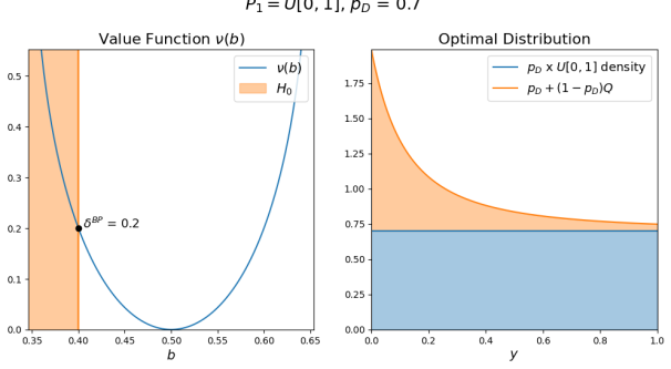
Figure 1: $\nu(b)$ and $p_{D}P_{1}+(1-pD)Q^{*}$, where $Q^{*}\in\textbf{P}^{0.4}$ minimizes selection.

Breakdown analysis can also be framed as an exercise in partial identification, as in Kline & Santos (2013), Masten & Poirier (2020), and Diegert et al. (2022). In this framing, the researcher considers assumptions of the form $d_{f}(P_{0},P_{1})\leq\delta$ for some $\delta>0$, which continuously relax the assumption $P_{0}=P_{1}$. The identified set for $\beta$ grows with $\delta$. As long as the identified set is a subset of $\textbf{B}\setminus\textbf{B}_{0}$, it is clear the researcher’s conclusion holds. The breakdown point $\delta^{BP}$ can then be defined as either the largest $\delta$ for which the identified set is contained in $\textbf{B}\setminus\textbf{B}_{0}$, or the smallest $\delta$ for which the identified set has nontrivial intersection with $\textbf{B}_{0}$ (the latter of which corresponds to the definition given in display (4)). For further discussion of this equivalent framing of the breakdown point, see appendix B.2.

The remainder of this paper constructs a $\sqrt{n}$-consistent and asymptotically normal estimator of $\delta^{BP}$, and constructs a lower confidence interval for $\delta^{BP}$. Researchers working with partially complete datasets should discuss the plausible amount of selection in their setting, and report the point estimate and the lower confidence interval for $\delta^{BP}$ for each asserted conclusion. This will make plain to readers which conclusions are more sensitive to missing data concerns, and whether crucial results are sufficiently robust.

2.4 Preview of results

The estimation proceeds by separating the optimizations in (4). Define the primal problem

$$\nu(b)=\inf_{Q\in\textbf{P}^{b}}d_{f}(Q\|P_{1})$$ (5)

and notice that $\delta^{BP}=\inf_{b\in\textbf{B}_{0}}\nu(b)$. The first step is to estimate the value function $\nu$ over a set $B\subseteq\textbf{B}$ large enough that $\inf_{b\in\textbf{B}_{0}}\nu(b)=\inf_{b\in B\cap\textbf{B}_{0}}\nu(b)$, while the second step estimates $\delta^{BP}$ through a simple plug-in estimator.

The primal problem is an infinite dimensional convex optimization problem over the space of probability distributions, but one that is very well studied in convex analysis. In particular, when $\textbf{P}^{b}$ defined in display (3) is characterized by a finite number of moment conditions, the primal problem has a well behaved, finite-dimensional dual problem with the same value function (Borwein & Lewis, 1991, 1993; Csiszár et al., 1999; Broniatowski & Keziou, 2006). Section 3 discusses this dual problem and the assumptions needed to make use of it. Under regularity conditions discussed in Section 4, sample analogue estimators based on this dual problem are uniformly consistent and asymptotically Gaussian on compact sets. Differentiability of the infimum then implies convergence in distribution of the plug-in estimator.

To conclude this section, Assumption 1 collects conditions on the setting, the GMM model, and the $f$-divergence used to measure selection.

Assumption 1 (Setting).

$\{(D_{i},D_{i}Y_{i},X_{i})\}_{i=1}^{n}$ is an i.i.d. sample from a distribution satisfying

1. $p_{D}=P(D=1)\in(0,1)$,

2. $X\mid D=1$ and $X\mid D=0$ have the same finite support $\{x_{1},\ldots,x_{K}\}$,

3. $E\left[\sup_{b\in\boldsymbol{B}}\lVert g(Z,b)\rVert\mid D=1\right]<\infty$, where $Z=(Y,X)$, and

4. $f:\mathbb{R}\rightarrow[0,\infty]$ is closed, proper, strictly convex, essentially smooth, takes its unique minimum of $f(t)=0$ at $t=1$, and satisfies $f(t)=\infty$ for all $t<0$. The interior of $\text{dom}(f)\equiv\{t\in\mathbb{R}\;;\;f(t)<\infty\}$, denoted $(\ell,u)$, satisfies $\ell<1<u$, and $f$ is twice continuously differentiable on $(\ell,u)$.

The finite support condition (ii) ensures that $\textbf{P}^{b}$ is characterized by a finite number of moments (see remark 2.3 below for additional discussion). Condition (iv) ensures the $f$-divergence used to measure selection is well behaved, and is satisfied by every divergence in Table 1. In particular, strict convexity of $f$ ensures the primal problem (5) has a unique solution ($P_{1}$-almost surely). $f$ is required to be essentially smooth to ensure the dual problem has a unique solution. The requirements that $f(x)$ take a unique minimum of $0$ at $x=1$ and $f(x)=\infty$ for $x<0$ ensures that $d_{f}(Q\|P)$ is a well defined $f$-divergence.

Remark 2.3.

If $X$ is not finitely valued, it is easy to see that requiring $Q_{X}$ match a finite number of moments of $P_{0X}$ will estimate a value no larger than $\delta^{BP}$. If this value is large enough to assuage missing data concerns, the breakdown point can only be larger.

3 Duality

As defined in display (5), $\nu(b)$ is the value function of an infinite dimensional convex optimization problem. Fortunately, when selection is measured with an $f$-divergence, this minimization becomes a well-studied problem known by various names: maximal entropy (Csiszár et al. (1999)), partially finite programming (Borwein & Lewis (1991)), or simply $f$-divergence projection (Broniatowski & Keziou (2006)). The convex analysis results in these papers connect the primal problem in display (5) to a finite dimensional dual problem that is much easier to study and estimate. Under mild conditions, the value function of this dual problem coincides with the value function of the primal.

To state the dual problem, first note that the primal can be viewed as a problem over the set of densities with respect to $P_{1}$:

$$\nu(b)= \inf_{q}E\left[f(q(Y,X))\mid D=1\right]$$

$$\text{s.t. }E[h(Y,X,b)q(Y,X)\mid D=1]=c(b)$$

where

$$h(z,b)=h(y,x,b)=\begin{pmatrix}g(y,x,b)\\ \mathbbm{1}\{x=x_{1}\}\\ \vdots\\ \mathbbm{1}\{x=x_{K}\}\end{pmatrix}, c(b)=\begin{pmatrix}\frac{-p_{D}}{1-p_{D}}E[g(Y,X,b)\mid D=1]\\ P(X=x_{1}\mid D=0)\\ \vdots\\ P(X=x_{K}\mid D=0)\end{pmatrix},$$ (6)

The dual problem corresponding to (5) is given by

$$V(b)\equiv\sup_{\lambda\in\mathbb{R}^{d_{g}+K}}\lambda^{\intercal}c(b)-E\left[f^{*}\left(\lambda^{\intercal}h(Y,X,b)\right)\mid D=1\right]$$ (7)

where $f^{*}$ is the convex conjugate of $f$, given by $f^{*}(r)\equiv\sup_{t\in\mathbb{R}}\{rt-f(t)\}$. For convenience, table 2 summarizes the convex conjugate for several common divergences.

Table 2: Common $f$-divergence conjugates and effective domains

Name	$f(t)$	$\ell$, $u$	$f^{*}(r)$	$\ell^{*}$, $u^{*}$
Squared Hellinger	$\frac{1}{2}(\sqrt{t}-1)^{2}$	$\ell=0$, $u=\infty$	$\frac{1}{2}\left(\frac{1}{1-2r}-1\right)$	$\ell^{*}=-\infty$, $u^{*}=1/2$
Kullback-Leibler	$t\log(t)-t+1$	$\ell=0$, $u=\infty$	$\exp(r)-1$	$\ell^{*}=-\infty$, $u^{*}=\infty$
“Reverse” KL	$-\log(t)+t-1$	$\ell=0$, $u=\infty$	$-\log(1-r)$	$\ell^{*}=-\infty$, $u^{*}=1$

Remark 3.1.

To ensure $q$ corresponds to a probability density, the constraints must enforce $\int q(z)dP(z)=1$. This is implied by the constraints ensuring $Q_{X}=P_{0X}$ when $X$ is present. If there are no always-observed variables, set $h(z,b)=\begin{pmatrix}g(z,b)^{\intercal}&1\end{pmatrix}^{\intercal}\in\mathbb{R}^{d_{g}+1}$ and $c(b)=\begin{pmatrix}\frac{-p_{D}}{(1-p_{D})}E[g(Y,X,b)\mid D=1]^{\intercal}&1\end{pmatrix}^{\intercal}$.

3.1 Weak and strong duality

Assumption 1 suffices to show $V(b)\leq\nu(b)$. This fact is known as weak duality, and implies that

$$\inf_{b\in B\cap\textbf{B}_{0}}V(b)\leq\inf_{b\in B\cap\textbf{B}_{0}}\nu(b)=\delta^{BP}$$ (8)

for any $B\subseteq\textbf{B}$. This inequality shows that using the dual problem for estimation of the breakdown point is at worst conservative. If $\inf_{b\in B\cap\textbf{B}_{0}}V(b)$ is large enough to assuage selection concerns, researchers are assured that the breakdown point can only be larger.

Assuming only slightly more ensures strong duality holds, that is, $V(b)=\nu(b)$. Recall from Assumption 1 (iv) that the interior of $\text{dom}(f)=\{t\in\mathbb{R}\;;\;f(t)<\infty\}$ is denoted $(\ell,u)$.

Assumption 2 (Strong duality).

$B\subseteq\textbf{B}$ is convex, compact, and satisfies $\inf_{b\in\textbf{B}_{0}}\nu(b)=\inf_{b\in B\cap\textbf{B}_{0}}\nu(b)$. Furthermore, for each $b\in B$,

1. there exists $Q^{b}\in\textbf{P}^{b}$ such that $\ell<\frac{\partial Q^{b}}{\partial P_{1}}(z)<u$, almost surely $P_{1}$, and

2. $\lambda(b)$ solving (7) is in the interior of $\{\lambda\;;\;E[\lvert f^{*}(\lambda^{\intercal}h(Z,b))\rvert\mid D=1]<\infty\}$.

That strong duality holds under these conditions is a well known result.

Theorem 3.1 (Strong duality).

Suppose assumptions 1 and 2 hold. Then for each $b\in B$, $\nu(b)=V(b)$, with dual attainment.

The first order condition of the dual problem (7) provides intuition. Exchanging expectation and differentiation, the first order condition is

$$\begin{pmatrix}\frac{-p_{D}}{1-p_{D}}E_{P_{1}}[g(Y,X,b)]\\ P(X=x_{1}\mid D=0)\\ \vdots\\ P(X=x_{K}\mid D=0)\end{pmatrix}=E_{P_{1}}\left[(f^{*})^{\prime}\left(\lambda(b)^{\intercal}h(Y,X,b)\right)\begin{pmatrix}g(Y,X,b)\\ \mathbbm{1}\{X=x_{1}\}\\ \vdots\\ \mathbbm{1}\{X=x_{K}\}\end{pmatrix}\right]$$

where $\lambda(b)\in\mathbb{R}^{d_{g}+K}$ solves the dual problem. Consider $(f^{*})^{\prime}(\lambda(b)^{\intercal}h(y,x,b))$ as a density with respect to $P_{1}$. Notice that the first $d_{g}$ equations of the first order condition ensure $p_{D}E_{P_{1}}[g(Y,X,b)]+(1-p_{D})E_{P_{1}}[(f^{*})^{\prime}\left(\lambda(b)^{\intercal}h(Y,X,b)\right)g(Y,X,b)]=0$, while the remaining $K$ equalities ensure the marginal distribution of $X$ matches $P_{0X}$. In fact, the proof of theorem 3.1 shows that under assumptions 1 and 2, $(f^{*})^{\prime}\left(\lambda(b)^{\intercal}h(y,x,b)\right)$ is the $P_{1}$-density of the solution to the primal problem.

Assumption 2 ensures the set on which $\nu$ is estimated is large enough to estimate the breakdown point, but not so large as to contain parameter values that cannot be rationalized with a well behaved $P_{1}$-density. To illustrate, consider again example 2.1. $Y$ is a scalar, $\beta=E[Y]=p_{D}E_{P_{1}}[Y]+(1-p_{D})E_{P_{0}}[Y]$, and $P_{1}$ is $\mathcal{U}[0,1]$. For tractability suppose that Kullback-Leibler is used to measure selection. Since $P_{0}$ takes values on $[0,1]$, the Manski bounds for $\beta$ are $\left[\frac{p_{D}}{2},1-\frac{p_{D}}{2}\right]$. Appendix E.1 shows that strong duality is satisfied whenever $b\in\left(\frac{p_{D}}{2},1-\frac{p_{D}}{2}\right)$. Thus for this example, $B$ can be any convex, compact set in the interior of the Manski bounds.

Assumption 2 is maintained throughout the remainder of the paper. Accordingly, the notation $\nu$ will be used for the value function of the dual problem as well.

4 Estimation

4.1 The estimator

The sample analogue of the dual problem provides an estimator of the value function, and suggests a simple plug-in estimator of the breakdown point. The asymptotic properties of these estimators are easier to study if the objective of the dual problem is expressed with a single unconditional expectation, which comes at the cost of additional notation.

First define the matrix $J(D)=\begin{bmatrix}-DI_{d_{g}}&0\\ 0&(1-D)I_{K}\end{bmatrix}$ where $I_{d_{g}}$ and $I_{K}$ are identity matrices. Notice that $E\left[\frac{J(D)h(DY,X,b)}{(1-p_{D})}\right]=c(b)$ and

$$\nu(b)=\sup_{\lambda\in\mathbb{R}^{d_{g}+K}}E\left[\frac{\lambda^{\intercal}J(D)h(DY,X,b)}{1-p_{D}}-\frac{Df^{*}\left(\lambda^{\intercal}h(DY,X,b)\right)}{p_{D}}\right].$$ (9)

Define

$$\varphi(D,DY,X,b,\lambda,p)\equiv\frac{\lambda^{\intercal}J(D)h(DY,X,b)}{1-p}-\frac{D}{p}f^{*}(\lambda^{\intercal}h(DY,X,b)),$$ (10)

and observe that the dual problem is $\sup_{\lambda\in\mathbb{R}^{d_{g}+K}}E[\varphi(D,DY,X,b,\lambda,p_{D})]$. The estimator of the value function is defined pointwise by

$$\hat{\nu}_{n}(b)\equiv\sup_{\lambda\in\mathbb{R}^{d_{g}+K}}\frac{1}{n}\sum_{i=1}^{n}\varphi(D_{i},D_{i}Y_{i},X_{i},b,\lambda,\hat{p}_{D,n}),$$ (11)

where $\hat{p}_{D,n}\equiv\frac{1}{n}\sum_{i=1}^{n}D_{i}$ estimates $p_{D}$. Finally, $\hat{\delta}_{n}^{BP}\equiv\inf_{b\in B\cap\textbf{B}_{0}}\hat{\nu}_{n}(b)$ estimates the breakdown point.

4.2 Asymptotic normality

The following assumption suffices for $\hat{\delta}_{n}^{BP}$ to be $\sqrt{n}$-consistent and asymptotically normal. First observe that the estimands $\theta_{0}(b)=(\nu(b),\lambda(b),p_{D})$ solve the moment conditions $E[\phi(D,DY,X,b,\theta_{0}(b))]=0$, where

$$\phi(D,DY,X,b,\theta)=\phi(D,DY,X,b,v,\lambda,p)=\begin{pmatrix}\varphi(D,DY,X,b,\lambda,p)-v\\ \nabla_{\lambda}\varphi(D,DY,X,b,\lambda,p)\\ D-p\end{pmatrix},$$ (12)

Let $\text{Gr}(\theta_{0})\equiv\left\{(b,\theta(b))\;;\;b\in B\right\}$ denote the graph of $\theta_{0}$. For $\eta>0$, the closed $\eta$-expansion about this graph is $\text{Gr}(\theta_{0})^{\eta}\equiv\left\{(b,\theta)\in B\times\mathbb{R}^{d_{g}+K+2}\;;\;\inf_{(b^{\prime},\theta^{\prime})\in\text{Gr}(\theta_{0})}\lVert(b,\theta)-(b^{\prime},\theta^{\prime})\rVert\leq\eta\right\}$.

Assumption 3 (Estimation).

Suppose that

1. $\textbf{B}_{0}$ is closed,

2. $\min_{b\in B\cap\textbf{B}_{0}}\nu(b)$ has a unique solution,

3. the matrix $E[h(Y,X,b)h(Y,X,b)^{\intercal}\mid D=1]$ is nonsingular for each $b\in B$,

4. $g(y,x,b)$ is continuously differentiable with respect to $b$ for each $(y,x)$, and

5. there exists a convex, compact set $\Theta^{B}$ containing $\text{Gr}(\theta_{0})^{\eta}$ for some $\eta>0$ satisfying

   $$E\left[\sup_{(b,\theta)\in\Theta^{B}}\lVert\phi(D,DY,X,b,\theta)\rVert^{2}\right]<\infty E\left[\left(\sup_{(b,\theta)\in\Theta^{B}}\lVert\nabla_{(b,\theta)}\phi(D,DY,X,b,\theta)\rVert\right)^{2}\right]<\infty.$$ and

As previewed in section 2.4, $\hat{\delta}_{n}^{BP}$ is viewed as a two-step estimator where $\hat{\nu}_{n}$ estimates $\nu$ in the first step, and $\hat{\delta}_{n}^{BP}=\inf_{b\in B\cap\textbf{B}_{0}}\hat{\nu}_{n}(b)$ is a plug-in estimator for $\delta^{BP}=\inf_{b\in B\cap\textbf{B}_{0}}\nu(b)$. Conditions (iii), (iv), and (v) imply $\sqrt{n}(\hat{\nu}_{n}-\nu)$ converges weakly in the space of bounded functions on $B$, to a limiting process that is almost surely continuous. This is shown by linearizing $0=\frac{1}{n}\sum_{i=1}^{n}\phi(D_{i},D_{i}Y_{i},X_{i},b,\hat{\theta}_{n}(b))$ uniformly over $b\in B$. Conditions (i) and (ii) ensure minimization over $B\cap\textbf{B}_{0}$ is a (Hadamard) differentiable map on the set of continuous functions of $B$. The delta method then implies $\sqrt{n}(\hat{\delta}_{n}^{BP}-\delta^{BP})$ converges in distribution to a normal distribution.

Assumption 3 (i) and (iv) are easily verified by inspection of $\textbf{B}_{0}$ and $g$ respectively. Conditions (iii) and (v) are similar to conditions required of generalized empirical likelihood estimators (see, e.g., Antoine & Dovonon (2021) assumption 1 (v) and assumption 3 (iv), (vii)). Assumption 3 (ii) deserves additional scrutiny. When $\textbf{B}_{0}$ is a convex set, condition (ii) holds when $\nu$ is a strictly convex function. The following lemma shows that this is the case when $g(y,x,b)$ describes a linear model with the outcome being the only missing data value.

Lemma 4.1 (Convex value function, linear models).

Suppose assumptions 1 and 2 hold, the sample is $\{D_{i},D_{i}Y_{i},X_{i1},X_{i2}\}_{i=1}^{n}$ where $Y_{i}\in\mathbb{R}$, $X_{i1}\in\mathbb{R}^{d_{x1}}$, and $X_{i2}\in\mathbb{R}^{d_{x2}}$, and the parameter $\beta$ is identified by

$$E[(Y-X_{1}^{\intercal}\beta)X_{2}]=0$$

Then $\hat{\nu}_{n}$ and $\nu$ are convex. If in addition $E[X_{2}X_{1}^{\intercal}]$ has full column rank, then $\nu$ is strictly convex.

Lemma 4.1 covers instrumental variable models directly, and ordinary least squares as a special case (by setting $X_{2}=X_{1}$). It also covers parameters of the form $\beta=E[\tilde{g}(Y,X)]$, because the OLS regression of $\tilde{g}(Y,X)$ on a constant recovers $E[\tilde{g}(Y,X)]$. Simulation evidence presented in appendix E suggests data generating processes and models not covered by lemma 4.1 also produce convex $\nu$. Remark 4.1 below discusses an approach to relaxing assumption 3 (ii), at the cost of additional complexity.

Theorem 4.2 below formally states the convergence in distribution result along with consistency of an estimator of the asymptotic variance. The variance depends on the jacobian term $\Phi(b)\equiv E[\nabla_{\theta}\phi(D,DY,X,b,\theta_{0}(b))]$, which is estimated with

$$\hat{\Phi}_{n}(b)\equiv\frac{1}{n}\sum_{i=1}^{n}\nabla_{\theta}\phi(D,DY,X,b,\hat{\theta}_{n}(b)),$$ (13)

where $\hat{\theta}_{n}(b)\equiv(\hat{\nu}_{n}(b),\hat{\lambda}_{n}(b),\hat{p}_{D,n})$ and $\hat{\lambda}_{n}(b)\equiv\operatorname*{arg\,max}_{\lambda\in\mathbb{R}^{d_{g}+K}}\frac{1}{n}\sum_{i=1}^{n}\varphi(D_{i},D_{i}Y_{i},X_{i},b,\lambda,\hat{p}_{D,n})$.

Theorem 4.2 (Asymptotic normality).

Suppose assumptions 1, 2, and 3 hold. Let $\hat{b}_{n}\equiv$
$\operatorname*{arg\,min}_{b\in B\cap\textbf{B}_{0}}\hat{\nu}_{n}(b)$ and

$$\hat{\sigma}_{n}^{2}\equiv\frac{1}{n}\sum_{i=1}^{n}\left((\hat{\Phi}_{n}(\hat{b}_{n})^{-1})^{(1)}\phi(D,DY,X,\hat{b}_{n},\hat{\theta}_{n}(\hat{b}_{n}))\right)^{2}$$

where $(\hat{\Phi}_{n}(\hat{b}_{n})^{-1})^{(1)}$ is the first row of the matrix $\hat{\Phi}_{n}(\hat{b}_{n})^{-1}$. Then $\sqrt{n}(\hat{\delta}_{n}^{BP}-\delta^{BP})/\hat{\sigma}_{n}\overset{d}{\rightarrow}N(0,1)$.

4.3 Inference

A large breakdown point implies the incomplete distribution $P_{0}$ would have to differ greatly from $P_{1}$ to rationalize the null hypothesis. If $\delta^{BD}$ is larger than the plausible amount of selection in the setting, the null hypothesis is similarly implausible. Skeptical readers following this argument may worry the point estimate $\hat{\delta}_{n}^{BP}$ is larger than $\delta^{BP}$ due to sample noise – but the force of the argument is only strengthened if $\hat{\delta}_{n}^{BP}$ falls below $\delta^{BP}$.

To address these concerns, researchers should report lower confidence intervals along with point estimates of the breakdown point. Theorem 4.2 implies that under assumptions 1, 2, and 3,

$$\widehat{CI}_{L,n}\equiv\hat{\delta}_{n}-\frac{\hat{\sigma}_{n}}{\sqrt{n}}c_{1-\alpha}$$ (14)

satisfies $\lim_{n\rightarrow\infty}P(\widehat{CI}_{L,n}\leq\delta^{BP})=1-\alpha$ when $c_{1-\alpha}$ is the $1-\alpha$ quantile of the standard normal distribution.

Remark 4.1.

Assumption 3 (ii) can be relaxed at the cost of additional complexity. Without assumption 3 (ii), $\sqrt{n}(\hat{\nu}_{n}-\nu)$ still converges in $\ell^{\infty}(B)$ to $\mathbb{G}_{\nu}$, a tight Gaussian process on $B$, and minimization of a function over $B\cap\textbf{B}_{0}$ remains a (Hadamard) directionally differentiable map on the set of continuous functions of $B$. The delta method continues to imply $\sqrt{n}(\hat{\delta}_{n}^{BP}-\delta^{BP})$ converges in distribution to $\inf_{b\in\textbf{m}(\nu)}\mathbb{G}_{\nu}(b)$, where $\textbf{m}(\nu)$ is the set of minimizers of $\nu$.

Given a bootstrap $\hat{\nu}_{n}^{*}$ such that $\sqrt{n}(\hat{\nu}_{n}^{*}-\hat{\nu}_{n})$ converges weakly in probability conditional on $\{D_{i},D_{i}Y_{i},X_{i}\}_{i=1}^{n}$ to $\mathbb{G}_{\nu}$, confidence intervals can still be constructed by utilizing the tools developed in Fang & Santos (2019). One approach is to estimate the set $\textbf{m}(\nu)$ through “near maximizers” of $\hat{\nu}_{n}$ and using this estimated set to form an estimator of the map $h\mapsto\inf_{b\in\textbf{m}(\nu)}h(b)$. The confidence interval for $\delta^{BP}$ is formed by replacing $\hat{\sigma}_{n}c_{1-\alpha}$ in display (14) with the $1-\alpha$ quantile of this estimated function applied to the bootstrap sample; see Fang & Santos (2019) theorem 3.2 and appendix lemma S.4.8.. As most cases of interest appear to satisfy assumption 3 (ii), this extension is left for future research.

5 Simulations

This section presents simulation results on a variety of different data generating processes. This serves both to illustrate the wide scope of models which can make use of breakdown point analysis and to investigate the finite sample properties of the proposed estimators. In each case, selection is measured using squared Hellinger divergence.

5.1 Simple mean

Recall example 2.1. The parameter of interest is the mean of a scalar random variable $Y$, $\beta=E[Y]=p_{D}E_{P_{1}}[Y]+(1-p_{D})E_{P_{0}}[Y]$, and the sample is $\{D_{i},D_{i}Y_{i}\}_{i=1}^{n}$. The distribution of $Y\mid D=1$ is the uniform distribution on $[0,1]$. The probability of observing $Y$ is $p_{D}=P(D=1)=0.7$. To support the claim $H_{1}\;:\;\beta>0.4$, let $H_{0}\;:\;\beta\leq 0.4$. Recall that the true breakdown point, $\delta^{BP}$, of this example is just over $0.2$.

The following table summarizes 1,000 simulations for several different sample size.

Table 3: Simulations, expectation

n	Bias	St. Dev.	Coverage	Ave. CI Length
1,000	0.005	0.056	98.5	0.090
3,000	0.002	0.032	96.3	0.051
5,000	0.001	0.025	95.8	0.039
10,000	0.001	0.017	95.8	0.028

The simulations show little bias. Coverage is slightly above the targeted 95% significance level in smaller samples.

5.2 Linear models

Linear models are the among the most common tools used by empirical researchers. This subsection uses simulations to investigate linear regression with exogenous regressors.

Consider the model

$$Y_{1}=\beta_{0}+\beta_{1}X_{1}+\beta_{2}Y_{2}+\beta_{3}X_{2}+\varepsilon=W^{\intercal}\beta+\varepsilon,$$ (15)

where $W=\begin{pmatrix}1&X_{1}&Y_{2}&X_{2}\end{pmatrix}^{\intercal}$ are the exogenous regressors: $E[W\varepsilon]=0$. Here $Y_{1}$ is a continuous outcome variable, $X_{1}=\{0,1\}$ is the regressor of interest, $Y_{2}$ is a continuously distributed control, and $X_{2}\in\{0,1,2\}$ is a discrete control. The conclusion to be investigated is that the coefficient on $X_{1}$ is positive:

$$H_{0}\;:\;\beta_{1}\leq 0, H_{1}\;:\;\beta_{1}>0$$ (16)

The researcher observes the sample $\{D_{i},D_{i}Y_{1i},D_{i}Y_{2i},X_{1i},X_{2i}\}_{i=1}^{n}$ and uses squared Hellinger to measure selection.

The data generating process specification takes inspiration from mincerian wage equations. For worker $i$, let $Y_{1i}$ be $i$’s log-income, $X_{1i}$ an indicator for $i$ being a college graduate, $Y_{2i}$ be $i$’s work experience, and $X_{2i}$ the number of parents with college degrees ($0$, $1$, or $2$). Specifically, let $X_{2}$ be multinomial, $X_{1}\sim\text{Binomial}\left(\frac{X_{2}+1}{4}\right)$, and $Y_{2}\sim\text{Beta}(3-X_{1},3)$. Let $\tilde{\varepsilon}\sim U[-1,1]$ (independent of all other variables), and $\varepsilon=(X_{1}+1)\tilde{\varepsilon}$. The coefficients are specified as $\beta_{0}=\beta_{1}=\beta_{2}=1$ and $\beta_{3}=0.5$. Finally, $Y_{1}$ is generated according to equation (15). Notice the support of $(Y_{1},Y_{2},X_{1},X_{2})$ is compact, ensuring the moment conditions in assumption 3 (v) are satisfied.

For the missing data process, let $D=\mathbbm{1}\{\varepsilon X_{1}+10X_{1}+5(X_{2}-1)>\eta\}$, where $\eta\sim N(\mu_{\eta},\sigma_{\eta}^{2})$. The population value of the breakdown point is approximated as the point estimate obtained from a sample with one million observations. This sample reveals $P(D=1)$ is about $0.71$, and suffers from selection. Specifically, ignoring the incomplete observations is equivalent to solving $\frac{1}{n}\sum_{i=1}^{n}\frac{D_{i}}{\hat{p}_{D,n}}(Y_{i}-W_{i}^{\intercal}\hat{\beta}_{n}^{MCAR})W_{i}=0$ for $\hat{\beta}_{n}^{MCAR}$, which results in $\hat{\beta}_{n}^{MCAR}=(1.04,1.37,1.02,0.42)$. The estimated squared Hellinger distance between $P_{0X}$ and $P_{1X}$ is $0.081$. This large sample suggests the breakdown point of the conclusion described in display (16) is about 0.163.

The following table summarizes 1,000 simulations for several different sample sizes.

Table 4: Simulations, OLS

n	Bias	St. Dev.	Coverage	Ave. CI Length
1,000	0.016	0.049	98.7	0.076
3,000	0.007	0.026	95.8	0.041
5,000	0.004	0.019	95.5	0.031
10,000	0.003	0.013	94.5	0.022

Once again the simulations show little bias, with coverage slightly above the targeted 95% significance level in smaller samples.

5.3 Logistic regression

The logistic model is a popular choice for estimating the conditional probability of an event. Let $Z=(Z_{1},Z_{-1})\in\{0,1\}\times\mathbb{R}^{d}$ and suppose that $P(Z_{1}=1\mid Z_{-1})=\Lambda(Z_{-1}^{\intercal}\beta)$, where $\Lambda(t)\equiv\frac{\exp(t)}{1+\exp(t)}$. The log-likelihood is concave, so estimating this model through maximum likelihood is equivalent to solving the first order condition

$$E[(Z_{1}-\Lambda(Z_{-1}^{\intercal}\beta))Z_{-1}]=0.$$

The model can be viewed as nonlinear GMM, with moment function $g(z,b)=(z_{1}-\Lambda(z_{-1}^{\intercal}b))z_{-1}$.

This simulation considers the model’s prediction for $P(Z_{1}=1\mid Z_{-1}=\bar{z})=\Lambda(\bar{z}^{\intercal}\beta)$ for a known $\bar{z}$, and investigates the robustness of the conclusion that this conditional probability is at least 0.5. The corresponding null and alternative hypotheses are

$$H_{0}:\Lambda(\bar{z}^{\intercal}\beta)\leq 0.5, H_{1}:\Lambda(\bar{z}^{\intercal}\beta)>0.5.$$ (17)

Simulation evidence presented in appendix E.3 suggests the data generating process described below produces a convex value function. Since $H_{0}$ is equivalent to $\bar{z}^{\intercal}\beta\leq\ln(0.5)-\ln(1-0.5)=0$ and is therefore convex, this suggests that assumption 3 (ii) holds.

The data generating process is one where the outcome is always observed, and the explanatory variables are sometimes missing. Specifically, $Y=Z_{-1}\in\mathbb{R}^{3}$ is constructed by drawing $\tilde{Y}\sim N(0,\Omega)$ and setting $Y^{(j)}=2\times(\Phi(\tilde{Y}^{(j)})-0.5)$; the result is that each $Y^{(j)}$ has uniform marginal distributions on $[-1,1]$, and nontrivial covariance matrix. The outcome is always-observed: $X=Z_{1}$. The true underlying coefficients are $\beta=(1,-1,0.1)$, and the missing data process is conditionally binomial with $P(D=1\mid X=x,Y=y)=\max\{0.8-X,Y^{(3)}/2+0.5\}$; that is, the probability of a complete observation is at least $0.8$ when $X=1$ and grows weakly with $Y_{3}$.

The resulting samples suffer from selection. A sample with one million observations suggests that $P(D=1)$ is about $0.65$. Ignoring the incomplete observations is equivalent to solving $\frac{1}{n}\sum_{i=1}^{n}\frac{D}{\hat{p}_{D,n}}g(D_{i}Y_{i},X_{i},\hat{\beta}_{n}^{MCAR})=0$, which results in $\hat{\beta}_{n}^{MCAR}=(1,-1,0.79)$. The estimated squared Hellinger distance between $P_{0X}$ and $P_{1X}$ is $0.076$. The covariate value of interest is $\bar{y}=(-0.35,-0.25,0.5)$. The true value for $\Lambda(\bar{y}^{\intercal}\beta)$ is $0.488$, while the estimate assuming using the complete observations of the large sample above is $\Lambda(\bar{y}^{\intercal}\hat{\beta}_{n}^{MCAR})=0.573$. The point estimate for the breakdown point described by (17) using this large sample is $0.108$. This is treated as the truth when evaluating the 1,000 simulations per sample size summarized in the following table:

Table 5: Simulations, logistic

n	Bias	St. Dev.	Coverage	Ave. CI Length
1,000	0.003	0.018	94.5	0.029
3,000	-0.000	0.010	96.1	0.017
5,000	0.001	0.008	94.8	0.013
10,000	-0.000	0.005	95.9	0.009

These simulations shows essentially zero bias and correct coverage at relatively small sample sizes.

6 Conclusion

This paper proposes breakdown point analysis as a tractable approach to assessing the sensitivity of a researcher’s conclusion to the common MCAR assumption. When defined with squared Hellinger, the breakdown point $\delta^{BP}$ has a natural interpretation: if the result were false, the variables under study ($Z$) would have to predict an observation being selected into the sample ($D$) at least well enough that $H^{2}(P_{0},P_{1})=1-E[\sqrt{\text{Var}(D\mid Z)}]/\sqrt{\text{Var}(D)}\geq\delta^{BP}$. Estimators based on the sample analogue of the dual problem are shown $\sqrt{n}$-consistent and asymptotically normal, which facilitates the construction of lower confidence intervals. Researchers working with incomplete datasets should report the breakdown point estimate and lower confidence interval along with standard results, making transparent to their audience how robust the conclusion is to relaxing the MCAR assumption.

Appendices

Appendix A Appendix: notation

This appendix summarizes notation and facts used throughout the paper and appendices.

A.1 Calculations

A number of expressions are useful for verifying conditions in proofs and programming estimators. These are collected here for convenience.

Recall that $\theta_{0}(b)=(\nu(b),\lambda(b),p_{D})$, where $\nu(b)$ is the population value of the value function, $\lambda(b)$ is the corresponding Lagrange multiplier, and $p_{D}=P(D=1)$. The notation $\theta=(v,\lambda,p)\in\mathbb{R}^{d_{g}+K+2}$ refers to a vector in Euclidean space.

$$\varphi(D,DY,X,b,\lambda,p) \equiv\frac{\lambda^{\intercal}J(D)h(DY,X,b)}{1-p}-\frac{D}{p}f^{*}(\lambda^{\intercal}h(DY,X,b))$$ (18)

$$\phi(D,DY,X,b,\theta) =\phi(D,DY,X,b,v,\lambda,p)\equiv\begin{pmatrix}\varphi(D,DY,X,b,\lambda,p)-v\\ \nabla_{\lambda}\varphi(D,DY,X,b,\lambda,p)\\ D-p\end{pmatrix},$$ (19)

$$\Phi(b) =E[\nabla\phi(D,DY,X,b,\theta_{0}(b))]$$ (20)

$$\nabla_{\theta}\phi(d,dy,x,b,\theta) =\nabla_{v,\lambda,p}\begin{pmatrix}\varphi(d,dy,x,b,\lambda,p)-v\\ \nabla_{\lambda}\varphi(d,dy,b,\lambda,p)\\ d-p\end{pmatrix}$$

$$=\begin{bmatrix}-1&\nabla_{\lambda}\varphi(d,dy,x,b,\lambda,p)^{\intercal}&\nabla_{p}\varphi(d,dy,x,b,\lambda,p)\\ 0&\nabla_{\lambda}^{2}\varphi(d,dy,x,b,\lambda,p)&\nabla_{p}\nabla_{\lambda}\varphi(d,dy,x,b,\lambda,p)\\ 0&0&-1\end{bmatrix}$$ (21)

$$\nabla_{\lambda}\varphi(d,dy,x,b,\lambda,p) =\frac{J(d)h(dy,x,b)}{1-p}-\frac{d}{p}(f^{*})^{\prime}(\lambda^{\intercal}h(dy,x,b))h(dy,x,b)$$ (22)

$$\nabla_{\lambda}^{2}\varphi(d,dy,x,b,\lambda,p) =-\frac{d}{p}(f^{*})^{\prime\prime}(\lambda^{\intercal}h(dy,x,b))h(dy,x,b)h(dy,x,b)^{\intercal}$$

$$\nabla_{p}\varphi(d,dy,x,b,\lambda,p) =\frac{\lambda^{\intercal}J(d)h(dy,x,b)}{(1-p)^{2}}+\frac{d}{p^{2}}f^{*}(\lambda^{\intercal}h(dy,x,b))$$

$$\nabla_{p}\nabla_{\lambda}\varphi(d,dy,x,b,\lambda,p) =\frac{J(d)h(dy,x,b)}{(1-p)^{2}}+\frac{d}{p^{2}}(f^{*})^{\prime}(\lambda^{\intercal}h(dy,x,b))h(dy,x,b)$$

A.2 Graphs

Let $X\subseteq\mathbb{R}^{d_{x}}$ and $Y\subseteq\mathbb{R}^{d_{y}}$. For a function $f:X\rightarrow Y$, the graph of the function refers to the set $\text{Gr}(f)=\left\{(x,f(x))\;;\;x\in X\right\}\subseteq X\times Y$. Define the closed $\delta$-expansion of the graph of $f$:

$$\text{Gr}(f)^{\delta}\equiv\left\{(x,y)\in X\times Y\;;\;\inf_{(x^{\prime},y^{\prime})\in\text{Gr}(f)}\lVert(x,y)-(x^{\prime},y^{\prime})\rVert\leq\delta\right\}$$

Note that $\text{Gr}(f)^{\delta}$ is closed, and bounded if $\text{Gr}(f)$ is bounded.

Given $Z\subseteq\mathbb{R}^{d_{z}}$ and $g:X\rightarrow Z$, one can view $(f,g)$ as a function from $X$ to $(Y,Z)$:

$$(f,g):X\rightarrow(Y,Z), (f,g)(x)=(f(x),g(x))$$

Define the graph of this function, $\text{Gr}(f,g)=\left\{(x,f(x),g(x))\;;\;x\in X\right\}\subseteq X\times Y\times Z$, and the closed $\delta$-expansion about this graph:

$$\text{Gr}(f,g)^{\delta}=\left\{(x,y,z)\in X\times Y\times Z\;;\;\inf_{(x^{\prime},y^{\prime},z^{\prime})\in\text{Gr}(f,g)}\lVert(x,y,z)-(x^{\prime},y^{\prime},z^{\prime})\rVert\leq\delta\right\}$$

Several easily constructed subsets of $\text{Gr}(f,g)^{\delta}$ imply useful inequalities. For example,

$$\inf_{(x^{\prime},y^{\prime},z^{\prime})\in\text{Gr}(f,g)}\lVert(x,y,g(x))-(x^{\prime},y^{\prime},z^{\prime})\rVert \leq\inf_{(x^{\prime},y^{\prime},z^{\prime})\in\text{Gr}(f,g)}\lVert(x,y,g(x))-(x^{\prime},y^{\prime},g(x))\rVert$$

$$=\inf_{(x,y)\in\text{Gr}(f)^{\delta}}\lVert(x,y)-(x^{\prime},y^{\prime})\rVert$$

implies $\left\{(x,y,g(x))\;;\;(x,y)\in\text{Gr}(f)^{\delta}\right\}\subseteq\text{Gr}(f,g)^{\delta}$. It follows that for a function $h:X\times Y\times Z\rightarrow\mathbb{R}$,

$$\sup_{(x,y)\in\text{Gr}(f)^{\delta}}h(x,y,g(x))\leq\sup_{(x,y,z)\in\text{Gr}(f,g)^{\delta}}h(x,y,z).$$

Similarly,

$$\lVert(x,y,z)-(x^{\prime},y^{\prime},z^{\prime})\rVert \leq\lVert(x,y,z)-(x^{\prime},y^{\prime},z)\rVert+\lVert(x^{\prime},y^{\prime},z)-(x^{\prime},y^{\prime},z^{\prime})\rVert$$

$$=\lVert(x,y)-(x^{\prime},y^{\prime})\rVert+\lVert z-z^{\prime}\rVert$$

implies that

$$\inf_{(x^{\prime},y^{\prime})\in\text{Gr}(f)^{\delta/2},\;z^{\prime}\in\text{Gr}(g)^{\delta/2}}\lVert(x,y,z)-(x^{\prime},y^{\prime},z^{\prime})\rVert$$

$$\hskip 56.9055pt\leq\inf_{(x^{\prime},y^{\prime})\in\text{Gr}(f)^{\delta/2}}\lVert(x,y)-(x^{\prime},y^{\prime})\rVert+\inf_{z^{\prime}\in\text{Gr}(g)^{\delta/2}}\lVert z-z^{\prime}\rVert.$$

It follows that $\left\{(x,y,z)\;;\;(x,y)\in\text{Gr}(f)^{\delta/2},\;(x,z)\in\text{Gr}(g)^{\delta/2}\right\}\subseteq\text{Gr}(f,g)^{\delta}$, and hence for a function $h:X\times Y\times Z\rightarrow\mathbb{R}$,

$$\sup_{(x,y)\in\text{Gr}(f)^{\delta/2},\;z\in\text{Gr}(g)^{\delta/2}}h(x,y,)\leq\sup_{(x,y,z)\in\text{Gr}(f,g)^{\delta}}h(x,y,z).$$

Finally, note that any constant $\bar{y}\in Y$ can be viewed as a trivial function of $X$. The graph of this function is the set $\text{Gr}(\bar{y})=\{(x,\bar{y})\;;\;x\in X\}$ and $\text{Gr}(\bar{y})^{\delta}$ is the set $\left\{(x,y)\;;\;x\in X,\lVert y-\bar{y}\rVert\leq\delta\right\}$.

A.3 Spaces of bounded functions

For any set $T$, $\ell^{\infty}(T)\equiv\left\{f:T\rightarrow\mathbb{R}\;;\;\sup_{t\in T}\lvert f(t)\rvert<\infty\right\}$ denotes the set of real-valued bounded functions on $T$. $\ell^{\infty}(T)$ is equipped with the sup-norm: for $f\in\ell^{\infty}(T)$, $\lVert f\rVert_{\infty}\equiv\lVert f\rVert_{T}\equiv\sup_{t\in T}\lvert f(t)\rvert$. The space of bounded functions taking values in $\mathbb{R}^{K}$ for some $K\in\mathbb{N}$ is the product space $\ell^{\infty}(T)^{K}=\underbrace{\ell^{\infty}(T)\times\ldots\times\ell^{\infty}(T)}_{K\text{ times }}$, but can also be viewed as a process on $\ell^{\infty}(T\times\{1,\ldots,K\})$. The latter notation makes it clear that standard empirical process results, typically stated for scalar-valued processes, apply.

If $(T,d)$ is a compact metric space, the extreme value theorem implies that continuous functions on $T$ are also bounded and hence form of a subpace of $\ell^{\infty}(T)$. This subspace is denoted

$$\mathcal{C}(T,d)=\{f:T\rightarrow\mathbb{R}\;;\;f\text{ is continuous}\}$$

the notation $\mathcal{C}(T)$ will be used to mean $\mathcal{C}(T,d)$ when the metric $d$ is clear from context.

Some results will refer to subsets of bounded functions whose graphs falls into a particular set. Specifically, let $E^{t}\subseteq\mathbb{R}^{d_{E}}$ for each $t\in T$, $E^{T}\equiv\{(t,e)\;;\;t\in T,e\in E^{t}\}$, and $\ell^{\infty}(T,E^{T})^{d_{E}}$ be the subset of $\ell^{\infty}(T)^{d_{E}}$ whose graph is a subset of $E^{T}$:

$$\ell^{\infty}(T,E^{T})^{d_{E}}=\left\{g:T\rightarrow\mathbb{R}^{d_{E}}\;;\;g(t)\in E^{t},\;\sup_{t\in T}\lVert g(t)\rVert<\infty\right\}\subset\ell^{\infty}(T)^{d_{E}}$$

For an example of how this will be used, let $\bar{x}>0$ and note that the function $f(t,e)=\ln(t+e)$ is uniformly continuous on the set $\{(t,e)\;;\;t+e\geq\bar{x}\}$. Defining $E^{t}=\{e\in\mathbb{R}\;;\;e\geq\bar{x}-t\}$ and $E^{T}$ as above, we have that $f(t,e)$ is uniformly continuous on this set. This implies that $\tilde{f}:\ell^{\infty}(T,E^{T})\rightarrow\ell^{\infty}(T)$ given by $\tilde{f}(g)(t)=f(t,g(t))=\ln(t+g(t))$ is continuous (see lemma D.1).

A.4 Matrices

For a matrix $A\in\mathbb{R}^{J\times K}$, let $\lVert A\rVert_{o}=\sup_{x\;;\;\lVert x\rVert_{2}=1}\lVert Ax\rVert_{2}$ be the operator norm of $A$, and $\lVert A\rVert_{\max}=\max_{ij}\lvert a_{ij}\rvert$, where $a_{ij}\in\mathbb{R}$ is the entry in the $i$-th row and $j$-th column of $A$. Let $\sigma_{1}(A)\geq\ldots\geq\sigma_{K}(A)\geq 0$ be the ordered singular values of $A$. For a square $K\times K$ real matrix $A$, let $\alpha_{1}(A)\geq\ldots\geq\alpha_{K}(A)$ be the ordered eigenvalues of $A$.

Recall that all norms on finite dimensional real vector spaces are strongly equivalent, meaning that if $\lVert\cdot\rVert_{1}$ and $\lVert\cdot\rVert_{2}$ are any norms on $\mathbb{R}^{J\times K}$, there exist constants $c,C>0$ such that $c\lVert A\rVert_{1}\leq\lVert A\rVert_{2}\leq C\lVert A\rVert_{1}$ for any matrix $A\in\mathbb{R}^{J\times K}$. If $A:T\rightarrow\mathbb{R}^{J\times K}$ for some set $T$, it follows that $E[\sup_{t}\lVert A(t)\rVert]<\infty$ for any norm if and only if $E[\sup_{t}\lVert A(t)\rVert_{\max}]<\infty$. Notice that strong equivalence with $\lVert\cdot\rVert_{\max}$ implies that, for any submatrix $\tilde{A}(t)$ of $A(t)$, $E[\sup_{t}\lVert A(t)\rVert]<\infty$ implies $E[\sup_{t}\lVert\tilde{A}(t)\rVert]<\infty$.

Recall that the singular values of a matrix $A\in\mathbb{R}^{J\times K}$ are related to the eigenvalues of the $K\times K$ square matrix $A^{\intercal}A$ by $\sigma_{k}(A)=\sqrt{\alpha_{k}(A^{\intercal}A)}$. The operator norm of a matrix is equal to its largest singular value, $\lVert A\rVert_{o}=\sigma_{1}(A)$, and for invertible matrix $A$ and any $k=1,\ldots,K$, $\frac{1}{\sigma_{k}(A)}$ is a singular value of $A^{-1}$. These imply $\lVert A^{-1}\rVert_{o}=\frac{1}{\sigma_{K}(A)}$. Finally, for a vector $x\in\mathbb{R}^{K}$, $\lVert xx^{\intercal}\rVert_{o}=\lVert x^{\intercal}x\rVert_{o}=\lVert x\rVert_{2}$.

Appendix B Appendix: measuring selection and breakdown analysis

B.1 Measuring selection

See 2.1

Proof.

The marginal, unconditional distribution of $Z$ is $P=p_{D}P_{1}+(1-p_{D})P_{0}$. This distribution dominates $P_{1}$ and $P_{0}$, which have densities

$$f_{1}(z)=\frac{P(D=1\mid Z=z)}{p_{D}}, f_{0}(z)=\frac{(1-P(D=1\mid Z=z))}{1-p_{D}},$$

with respect to $P$. This implies

$$H^{2}(P_{0},P_{1}) =\frac{1}{2}\int\left(\sqrt{f_{0}(z)}-\sqrt{f_{1}(z)}\right)^{2}dP(z)=\frac{1}{2}\left[\int f_{0}(z)+f_{1}(z)-2\sqrt{f_{1}(z)f_{0}(z)}dP(z)\right]$$

$$=1-\frac{\int\sqrt{P(D=1\mid Z=z)(1-P(D=1\mid Z=z))}dP(z)}{\sqrt{p_{D}(1-p_{D})}}$$

$$=1-\frac{E_{P}\left[\sqrt{\text{Var}(D\mid Z)}\right]}{\sqrt{\text{Var}(D)}}.$$

∎

B.2 Nominal identified sets

The exercise proposed in section 2.3 can also be understood with a framework of nominally identified sets. This approach to exposition is used in Kline & Santos (2013), Masten & Poirier (2020), and Diegert et al. (2022), and described for the current setting in this appendix.

Under the assumption $d(P_{0}\|P_{1})\leq\delta$ and $P_{0}\ll P_{1}$, the identified set for $\beta_{P}$ is a function of $\delta$:

$$\textbf{B}_{ID}(\delta)=\Big{\{}b\in\boldsymbol{B}\;;\;\exists Q,\;\;p_{D}\mathbb{E}_{P_{1}}[g(Z,b)]+(1-p_{D})\mathbb{E}_{Q}[g(Z,b)]=0,\text{ and }\;d(Q\;\|\;P_{1})\leq\delta\Big{\}}$$ (23)

Notice $\textbf{B}_{ID}(\delta)$ is always growing with $\delta$, in the sense that $\delta<\delta^{\prime}\implies\textbf{B}_{ID}(\delta)\subseteq\textbf{B}_{ID}(\delta^{\prime})$.

The researcher is primarily interested in testing $H_{0}\;:\;\beta\in\textbf{B}_{0}$ against $H_{1}\;:\;\beta\in\textbf{B}_{1}=\textbf{B}\setminus\textbf{B}_{0}$. Naturally, if $\textbf{B}_{ID}(\delta)$ has trivial intersection with $\textbf{B}_{0}$ she is confident in rejecting $H_{0}$. This leads to the question “what is the largest value of $\delta$ such that $\textbf{B}_{ID}(\delta)$ has empty intersection with $\textbf{B}_{0}$?” Formally, define the breakdown point as

$$\bar{\delta}^{BD}=\sup\left\{\delta\in\mathbb{R}_{+}\;;\;\textbf{B}_{ID}(\delta)\cap\textbf{B}_{0}=\varnothing\right\}$$ (24)

if $\textbf{B}_{ID}(0)\cap\textbf{B}_{0}=\varnothing$, otherwise define $\bar{\delta}^{BD}\coloneqq 0$.

B.2.1 Characterization through a value function

Lemma B.1 shows that the definition of the breakdown point given in (24) is equivalent to that given by (4).

Lemma B.1 (Characterization of breakdown point).

$$\inf_{b\in\boldsymbol{B}_{0}}\nu(b)=\bar{\delta}^{BD}$$

Proof.

Define the “robust region” as the set of $\delta\in\mathbb{R}_{+}$ where the identified set has trivial intersection with the null hypothesis:

$$RR=\{\delta\in\mathbb{R}_{+}\;;\;\textbf{B}_{ID}(\delta)\cap\textbf{B}_{0}=\varnothing\}$$

and let $RR^{c}=\mathbb{R}_{+}\setminus RR=\{\delta\in\mathbb{R}_{+}\;;\;\textbf{B}_{ID}(\delta)\cap\textbf{B}_{0}\neq\varnothing\}$ be its compliment in $\mathbb{R}_{+}$. Notice that

$$\bar{\delta}^{BD}=\begin{cases}\sup RR&\text{ if }RR\neq\varnothing\\ 0&\text{ otherwise}\end{cases}$$

The proof consists of two steps:

1. Showing that

   $$\bar{\delta}^{BD}=\inf RR^{c}$$ (25)

   where the infimum over the empty set is defined to be $\infty$.

2. Arguing that

   $$\inf_{b\in\boldsymbol{B}_{0}}\nu(b)\leq\inf RR^{c}, \inf_{b\in\boldsymbol{B}_{0}}\nu(b)\geq\inf RR^{c},$$ and

Step 1. is a consequence of $\textbf{B}_{ID}(\delta)$ being a growing set (in the sense that $\delta\leq\delta^{\prime}\implies\textbf{B}_{ID}(\delta)\subseteq\textbf{B}_{ID}(\delta^{\prime})$). Define $\bar{\delta}^{*}=\inf RR^{c}=\inf\{\delta\in\mathbb{R}_{+}\;;\;\textbf{B}_{ID}(\delta)\cap\textbf{B}_{0}\neq\varnothing\}$. There are three possibilities:

1. $\delta^{BD}=0$. Then $RR^{c}$ contains $(0,\infty)$, hence $0\leq\bar{\delta}^{*}=\inf RR^{c}\leq\inf(0,\infty)=0$.

2. $\delta^{BD}\in(0,\infty)$. Notice that $\delta\leq\delta^{\prime}\implies\textbf{B}_{ID}(\delta)\subseteq\textbf{B}_{ID}(\delta^{\prime})$ implies that $\delta\leq\delta^{\prime}\implies(\textbf{B}_{ID}(\delta)\cap\textbf{B}_{0})\subseteq(\textbf{B}_{ID}(\delta^{\prime})\cap\textbf{B}_{0})$, from which it follows that

   $$\delta\leq\delta^{\prime}\text{ and }\delta^{\prime}\in RR \implies \delta\in RR$$

   $$\delta\leq\delta^{\prime}\text{ and }\delta\in RR^{c} \implies \delta^{\prime}\in RR^{c}$$

   since $\bar{\delta}^{BD}\in(0,\infty)$, we have $RR$ contains $[0,\bar{\delta}^{BD})$. Similarly, $RR^{c}$ contains $(\bar{\delta}^{*},\infty)$, and since $RR\cap RR^{c}=\varnothing$, we have $\bar{\delta}^{BD}\leq\bar{\delta}^{*}$. For $n\in\mathbb{N}$, let $\delta_{n}\coloneqq\bar{\delta}^{*}-\frac{1}{n}\geq 0$, and notice that $\textbf{B}_{ID}(\delta_{n})\cap B=\varnothing$, equivalently, $\delta_{n}\in RR$. Therefore

   $$\bar{\delta}^{*}-\frac{1}{n}\leq\bar{\delta}^{BD}\leq\bar{\delta}^{*}$$

   let $n\rightarrow\infty$ to see that $\delta^{BD}=\delta^{*}$.

3. $\delta^{BD}=\infty$. Then the argument above implies $RR$ contains $[0,\infty)$, so $RR^{c}=\varnothing$ and $\delta^{*}=\infty$.

Therefore (25) holds.

For step 2., first notice that

$$\inf_{b\in\boldsymbol{B}_{0}}\nu(b)=\inf_{b\in\boldsymbol{B}_{0}}\inf_{Q\in\textbf{P}^{b}}d(Q\;\|\;P_{1})=\inf\bigcup_{b\in\boldsymbol{B}_{0}}\left\{d(Q\;\|\;P_{1})\;;\;Q\in\textbf{P}^{b}\right\}$$ (26)

If $\delta$ is such that $\textbf{B}_{ID}(\delta)\cap\textbf{B}_{0}\neq\varnothing$, then there exists $b\in\textbf{B}_{0}$ and $Q\in\textbf{P}^{b}$ such that $d(Q\;\|\;P_{1})\leq\delta$. This implies

$$\inf RR^{c}=\inf\left\{\delta\in\mathbb{R}_{+}\;;\;\textbf{B}_{ID}(\delta)\cap\textbf{B}_{0}\neq\varnothing\right\}\geq\inf\bigcup_{b\in\textbf{B}_{0}}\left\{d(Q\;\|\;P_{1})\;;\;K\in\textbf{P}^{b}\right\}$$

Conversely, for each real number $a$ satisfying $a=d(Q\;\|\;P_{1})$ for some $Q\in\textbf{P}^{b}$, $b\in\textbf{B}_{0}$, we have that $a\in\left\{\delta\;;\;\textbf{B}_{ID}(\delta)\cap\textbf{B}_{0}\neq\varnothing\right\}$. This implies

$$\inf\bigcup_{b\in\textbf{B}_{0}}\left\{d(Q\;\|\;P_{1})\;;\;Q\in\textbf{P}_{b}\right\}\geq\inf\left\{\delta\;;\;\textbf{B}_{ID}(\delta)\cap\textbf{B}_{0}\neq\varnothing\right\}=\inf RR^{c}$$

Putting (25), (26), and these two inequalities together we obtain

$$\inf_{b\in\textbf{B}_{0}}\nu(b) =\inf\bigcup_{b\in\textbf{B}_{0}}\left\{d(Q\;\|\;P_{1})\;;\;Q\in\textbf{P}^{b}\right\}=\inf\left\{\delta\;;\;\textbf{B}_{ID}(\delta)\cap\textbf{B}_{0}\neq\varnothing\right\}=\delta^{BD}$$

as was claimed. $\square$ ∎

Appendix C Appendix: proofs of duality results

Lemma C.1 (Unique primal solution).

Suppose $f$ is strictly convex on its domain, $p_{D}\in(0,1)$, and the infimum in (5) is finite. Then any solution attaining the infimum in (5) is unique, $P_{1}$-almost surely.

Proof.

Let $Q^{0},Q^{1}\in\textbf{P}^{b}$ attain the finite infimum in (5), and let $q^{0}$ and $q^{1}$ denote their densities with respect to $P_{1}$. We have that $\frac{-p_{D}}{(1-p_{D})}E_{P_{1}}[g(Y,X,b)]=E_{Q^{0}}[g(Y,X,b)]=E_{Q^{1}}[g(Y,X,b)]$ and $Q_{X}^{0}=Q_{X}^{1}=P_{0X}$. For any $\alpha\in(0,1)$, the measure $Q^{\alpha}=\alpha Q^{1}+(1-\alpha)Q^{0}\in\textbf{P}^{b}$ is feasible in (5), and characterized by the $P_{1}$-density $\alpha q^{1}+(1-\alpha)q^{0}$.

Suppose for contradiction that $Q^{0}$ and $Q^{1}$ differ on a set of positive $P_{1}$-measure. Strict convexity implies that for any $(y,x)$ in that set,

$$f(\alpha q^{1}(y,x)+(1-\alpha)q^{0}(y,x))<\alpha f(q^{1}(y,x))+(1-\alpha)q^{0}(y,x)$$

Integrating with respect to $P_{1}$ reveals $d_{f}(\alpha Q^{1}+(1-\alpha)Q^{0}\|P_{1})<\alpha d_{f}(Q^{1}\|P_{1})+(1-\alpha)d_{f}(Q^{0}\|P_{1})$, contradicting optimality of $Q^{0},Q^{1}$. ∎

Lemma C.2 (Weak duality).

Let $\nu(b)$ and $V(b)$ be as defined in (5) and (7), respectively. If assumption 1 holds, then $V(b)\leq\nu(b)$ for any $b\in\textbf{B}$.

Proof.

First note that if $\nu(b)=\infty$ the inequality holds trivially.

Suppose $\nu(b)<\infty$. Then $\textbf{P}^{b}\neq\varnothing$, hence there exists at least one density $q(z)=\frac{dQ}{dP_{1}}(z)$ satisfying $\int h(z,b)q(z)dP_{1}(z)=c(b)$. Notice that $f^{*}(r)=\sup_{t\in\mathbb{R}}\{rt-f(t)\}$ implies $f(t)+f^{*}(r)\geq f(t)+rt-f(t)=rt$. Use this to see that for any $Q\in\textbf{P}^{b}$ with $P_{1}$-density $q$,

$$f(q(z))+f^{*}(\lambda^{\intercal}h(z,b)) \geq\lambda^{\intercal}h(z,b)q(z)$$

$$\implies f(q(z)) \geq\lambda^{\intercal}h(z,b)q(z)-f^{*}(\lambda^{\intercal}h(z,b))$$

integrating over $z$ with respect to $P_{1}$ gives

$$\int f(q(z))dP_{1}(z) \geq\lambda^{\intercal}\underbrace{\int h(z,b)q(z)dP_{1}(z)}_{=c(b)}-\int f^{*}(\lambda^{\intercal}h(z,b))dP_{1}(z)$$

$$\implies d_{f}(Q\|P_{1}) \geq\lambda^{\intercal}c(b)-E\left[f^{*}(\lambda^{\intercal}h(z,b))\mid D=1\right]$$

the left hand side of the last inequality doesn’t depend on $\lambda\in\mathbb{R}^{d_{g}+K}$, while the right hand side doesn’t depend on $Q\in\textbf{P}^{b}$. Hence,

$$\nu(b)=\inf_{Q\in\textbf{P}^{b}}d_{f}(Q\|P_{1})\geq\sup_{\lambda\in\mathbb{R}^{d_{g}+K}}\left\{\lambda^{\intercal}c(b)-E\left[f^{*}(\lambda^{\intercal}h(Z,b))\mid D=1\right]\right\}=V(b).$$

∎

See 3.1

Proof.

Let M be the set of measurable functions mapping $z=(x,y)\mapsto\mathbb{R}$. Consider the relaxed problem

$$\tilde{\nu}(b) =\inf_{q\in\tilde{\textbf{P}}^{b}}\int f(q(y,x))dP_{1}(y,x)$$

$$\tilde{\textbf{P}}^{b} =\Bigg{\{}q\in\textbf{M}\;;\;\int h(y,x,b)q(y,x)dP_{1}(y,x)=c(b)\Bigg{\}}$$

for any $q\in\tilde{\textbf{P}}^{b}$, $K(\psi)=\int\psi(y,x)q(y,x)dP_{1}(y,x)$ is a (possibly signed) measure with total measure one. Notice this problem has the same objective as the primal problem (5), but a larger feasible set (the set of finite signed measures with total measure one).

Now apply Theorem II.2 of Csiszár et al. (1999), with trivial $\mathcal{K}=\{c(b)\}$. The dual of the relaxed problem is (7). Assumption 2 (i) is the “constraint qualification” of Csiszár et al. (1999) Theorem II.2, implying strong duality holds for the relaxed problem, $\tilde{\nu}(b)=V(b)$, and the dual problem’s value is attained at a maximum. Let $\lambda(b)$ solve the dual problem. Assumption 2 (ii) allows application of the second part of Theorem II.2, implying the solution to the relaxed problem is given by

$$q^{b}(y,x)=(f^{\prime})^{-1}(\lambda(b)^{\intercal}h(y,x,b))=(f^{*})^{\prime}(\lambda(b)^{\intercal}h(y,x,b))$$

By assumption 1 (iv) and Lemma C.1, this solution is unique $P_{1}$-almost surely.

Now we show that $q^{b}$ in fact solves the primal problem, (5). Notice $q^{b}$ is nonnegative, because $f^{\prime}$ is only defined on the non-negative reals. Furthermore,

$$\int q^{b}(x,y)dP_{1}(x,y) =\int\sum_{k=1}^{K}\mathbbm{1}\{x=x_{k}\}q^{b}(x,y)dP_{1}(x,y)$$

$$=\sum_{k=1}^{K}\int\mathbbm{1}\{x=x_{k}\}q^{b}(x,y)dP_{1}(x,y)$$

$$=\sum_{k=1}^{K}P(X=x_{k}\mid D=0)$$

$$=1$$

where the third equality follows from $\int h(y,x,b)q^{b}(x,y)dP_{1}(x,y)=c(b)$. So the measure $Q^{b}$ given by $Q^{b}(\psi)=\int\psi(y,x)q^{b}(y,x)dP_{1}(y,x)$ is a probability distribution dominated by $P_{1}$. Therefore $Q^{b}\in\textbf{P}^{b}$ is feasible in the primal problem (5). Being feasible in the primal and solving the relaxed problem, $Q^{b}$ must also solve the primal problem. ∎

Appendix D Appendix: proofs of estimation results

D.1 Technical lemmas

These results are self contained, with notation not related to the present paper.

Lemma D.1 (Uniform continuity of maps between bounded functions).

Let $T$ be a set, $E^{t}\subseteq\mathbb{R}^{d_{E}}$ for each $t\in T$, $E^{T}=\{(t,e)\;;\;t\in T,e\in E^{t}\}$, and $\ell^{\infty}(T,E^{T})^{d_{E}}$ be the subset of $\ell^{\infty}(T)^{d_{E}}$ whose graph is a subset of $E^{T}$:

$$\ell^{\infty}(T,E^{T})^{d_{E}}=\left\{g:T\rightarrow\mathbb{R}^{d_{E}}\;;\;g(t)\in E^{t},\;\sup_{t\in T}\lVert g(t)\rVert<\infty\right\}\subset\ell^{\infty}(T)^{d_{E}}$$

Let $f:E^{T}\rightarrow\mathbb{R}^{d_{f}}$ be such that $\sup_{t\in T}\lVert f(t,g(t))\rVert<\infty$ for any $g\in\ell^{\infty}(T,E^{T})^{d_{E}}$, and define

$$\tilde{f}:\ell^{\infty}(T,E^{T})^{d_{E}}\rightarrow\ell^{\infty}(T)^{d_{f}}, \tilde{f}(g)(t)=f(t,g(t)).$$

If $\{f(t,\cdot)\}_{t\in T}$ is uniformly equicontinuous, then $\tilde{f}$ is uniformly continuous.

Proof.

Let $\varepsilon>0$, and use uniform equicontinuity to choose $\delta>0$ such that

$$\lvert e_{1}-e_{2}\rvert<\delta\implies\lvert f(t,e_{1})-f(t,e_{2})\rvert<\varepsilon/2$$

for any $t\in T$. Notice that if $g_{1},g_{2}\in\ell^{\infty}(T,E^{T})^{d_{E}}$ with $\lVert g_{1}-g_{2}\rVert_{T}=\sup_{t\in T}\lvert g_{1}(t)-g_{2}(t)\rvert<\delta$, then

$$\lVert\tilde{f}(g_{1})-\tilde{f}(g_{2})\rVert_{T}=\sup_{t\in T}\lvert f(t,g_{1}(t)-f(t,g_{2}(t))\rvert\leq\varepsilon/2<\varepsilon$$

and hence $\lVert g_{1}-g_{2}\rVert_{T}<\delta\implies\lVert\tilde{f}(g_{1})-\tilde{f}(g_{2})\rVert_{T}<\varepsilon$. ∎

Remark D.1.

Lemma D.1 implies many simpler special cases. For example, suppose that for all $t,t^{\prime}\in T$, $f(t,e)=f(t^{\prime},e)$ and $E^{t}=E\subseteq\mathbb{R}$. Then lemma D.1 simplifies to: if $f:E\rightarrow\mathbb{R}$ is uniformly continuous, then $\tilde{f}:\ell^{\infty}(T)\rightarrow\ell^{\infty}(T)$ defined pointwise by $\tilde{f}(g)(t)=f(g(t))$ is continuous.

Lemma D.2 (Restricted infimum is uniformly continuous).

For any $A\subseteq T$ and any $f,g\in\ell^{\infty}(T)$,

$$\left\lvert\inf_{t\in A}f(t)-\inf_{t\in A}g(t)\right\rvert\leq\sup_{t\in A}\lvert f(t)-g(t)\rvert$$

as a result, $\iota:\ell^{\infty}(T)\rightarrow\mathbb{R}$ given by $\iota(h)=\inf_{t\in A}h(t)$ is uniformly continuous.

Proof.

Notice that

$$\sup_{t\in A}f(t)-\sup_{t\in A}g(t) \leq\sup_{t\in A}\{f(t)-g(t)\}\leq\sup_{t\in A}\lvert f(t)-g(t)\rvert,\text{ and }$$

$$-\left[\sup_{t\in A}f(t)-\sup_{t\in A}g(t)\right]=\sup_{t\in A}g(t)-\sup_{t\in A}f(t) \leq\sup_{t\in A}\{g(t)-f(t)\}\leq\sup_{t\in A}\lvert g(t)-f(t)\rvert=\sup_{t\in A}\lvert f(t)-g(t)\rvert,$$

hence $-\sup_{t\in A}\lvert f(t)-g(t)\rvert\leq\sup_{t\in A}f(t)-\sup_{t\in A}g(t)\leq\sup_{t\in A}\lvert f(t)-g(t)\rvert$, or equivalently

$$\left\lvert\sup_{t\in A}f(t)-\sup_{t\in A}g(t)\right\rvert\leq\sup_{t\in A}\lvert f(t)-g(t)\rvert.$$

Use this to see the claimed inequality:

$$\left\lvert\inf_{t\in A}f(t)-\inf_{t\in A}g(t)\right\rvert =\left\lvert-\sup_{t\in A}\{-f(t)\}-\left(-\sup_{t\in A}\{-g(t)\}\right)\right\rvert=\left\lvert\sup_{t\in A}\{-g(t)\}-\sup_{t\in A}\{-f(t)\}\right\rvert$$

$$\leq\sup_{t\in A}\lvert-g(t)-\{-f(t)\}\rvert=\sup_{t\in A}\lvert f(t)-g(t)\rvert.$$

Regarding the continuity claim, let $\varepsilon>0$ and set $\delta=\varepsilon$. Then

$$\lvert\iota(f)-\iota(g)\rvert\leq\sup_{t\in A}\lvert f(t)-g(t)\rvert\leq\sup_{t\in T}\lvert f(t)-g(t)\rvert=\lVert f-g\rVert_{T},$$

hence $\lVert f-g\rVert_{T}<\delta$ implies $\lvert\iota(f)-\iota(g)\rvert<\varepsilon$. ∎

Lemma D.3 (Restricted infimum is Hadamard directionally differentiable).

Let $(T,d)$ be a metric space, $A$ a compact subset of $T$, and

$$\iota:\ell^{\infty}(T)\rightarrow\mathbb{R}, \iota(f)=\inf_{t\in A}f(t)$$

Then $\iota$ is Hadamard directionally differentiable at any $f\in\mathcal{C}(T,d)$ tangentially to $\mathcal{C}(T,d)$. $\Psi_{A}(f)=\operatorname*{arg\,min}_{t\in A}f(t)$ is nonempty, and the directional derivative is given by

$$\iota_{f}^{\prime}:\mathcal{C}(T,d)\rightarrow\mathbb{R}, \iota_{f}^{\prime}(h)=\inf_{t\in\Psi_{A}(f)}h(t)$$

If $\Psi_{A}(f)$ is the singleton $\{t_{f}\}$, then $\iota$ is fully Hadamard differentiable at $f$ tangentially to $\mathcal{C}(T,d)$ and $\iota_{f}^{\prime}(h)=h(t_{f})$.

Proof.

The result is essentially a corollary of Fang & Santos (2019) Lemma S.4.9, which shows that $\phi:\ell^{\infty}(A)\rightarrow\mathbb{R}$ given by $\phi(f)=\sup_{t\in A}f(t)$ is Hadamard directionally differentiable at any $f\in\mathcal{C}(A,d)$ tangentially to $\mathcal{C}(A,d)$, with directional derivative

$$\phi_{f}^{\prime}:\mathcal{C}(A,d)\rightarrow\mathbb{R}, \phi_{f}^{\prime}(h)=\sup_{t\in\Psi_{A}(f)}h(t).$$

See Fang & Santos (2019) definition 2.1 for definitions of Hadamard directionally differentiable and fully Hadamard differentiable.

Let $f\in\mathcal{C}(T,d)$ and note that $\Psi_{A}(f)=\operatorname*{arg\,min}_{t\in A}f(t)$ is nonempty by the extreme value theorem. Let $\{h_{n}\}_{n=1}^{\infty}\subseteq\ell^{\infty}(T)$ and $\{r_{n}\}_{n=1}^{\infty}\subseteq\mathbb{R}_{+}$ be such that $h_{n}\rightarrow h\in\mathcal{C}(T,d)$ and $r_{n}\downarrow 0$. For $g\in\ell^{\infty}(T)$, let $g_{A}:A\rightarrow\mathbb{R}$ be the restriction of $g$ to $A$, given by $g_{A}(t)=g(t)$. Observe that $g\in\mathcal{C}(T,d)$ implies $g_{A}\in\mathcal{C}(A,d)$. Now notice that

$$\left\lvert\frac{\iota(f+r_{n}h_{n})-\iota(f)}{r_{n}}-\iota_{a}^{\prime}(h)\right\rvert$$

$$\hskip 28.45274pt=\left\lvert\frac{\inf_{t\in A}\{f(t)+r_{n}h_{n}(t)\}-\inf_{t\in A}f(t)}{r_{n}}-\inf_{t\in\Psi_{A}(f)}h(t)\right\rvert$$

$$\hskip 28.45274pt=\left\lvert\frac{-\sup_{t\in A}\{-f(t)-r_{n}h_{n}(t)\}-\left(-\sup_{t\in A}\{-f(t)\}\right)}{r_{n}}-\left(-\sup_{t\in\Psi_{A}(f)}\{-h(t)\}\right)\right\rvert$$

$$\hskip 28.45274pt=\left\lvert\frac{\sup_{t\in A}\{-f(t)+r_{n}\left(-h_{n}(t)\right)\}-\left(\sup_{t\in A}\{-f(t)\}\right)}{r_{n}}-\left(\sup_{t\in\Psi_{A}(f)}\{-h(t)\}\right)\right\rvert$$

$$\hskip 28.45274pt=\left\lvert\frac{\phi(-f_{A}+r_{n}(-h_{n,A}))-\phi(-f_{A})}{r_{n}}-\phi_{f}^{\prime}(-h_{A})\right\rvert,$$

where the last equality follows from the definitions and the fact that $\Psi_{A}(f)=\operatorname*{arg\,min}_{a\in A}f(a)=\operatorname*{arg\,max}_{a\in A}\{-f_{A}(a)\}$.

$h_{n}\rightarrow h\in h\in\mathcal{C}(T,d)$ implies $-h_{n,A}\rightarrow-h_{A}\in\mathcal{C}(A,d)$. Thus Fang & Santos (2019) Lemma S.4.9 and the definition of Hadamard directional differentiability implies

$$\lim_{n\rightarrow\infty}\left\lvert\frac{\iota(f+t_{n}h_{n})-\iota(f)}{t_{n}}-\iota_{a}^{\prime}(h)\right\rvert=\lim_{n\rightarrow\infty}\left\lvert\frac{\phi(-f_{A}+t_{n}(-h_{n,A}))-\phi(-f_{A})}{t_{n}}-\phi_{f}^{\prime}(-h_{A})\right\rvert=0.$$

Finally, if $\Psi_{A}(f)=\{t_{f}\}$ then $\inf_{t\in\Psi_{A}(f)}(h)=h(t_{f})$ is linear in $h$, and hence $\iota$ is fully Hadamard differentiable at $f$. ∎

Lemma D.4 (Uniform consistency of estimated moments).

Let $\mathcal{X}\subseteq\mathbb{R}^{d_{X}}$, $T\subseteq\mathbb{R}^{d_{T}}$, $E^{t}\subseteq\mathbb{R}^{d_{E}}$, $E^{T}=\{(t,e)\;;\;t\in T,e\in E^{t}\}$,

$$\hat{\gamma}_{n},\gamma:T\rightarrow\mathbb{R}^{d_{E}}, f:\mathcal{X}\times E^{T}\rightarrow\mathbb{R}^{K\times J}.$$ and

Suppose that

1. $\{X_{i}\}_{i=1}^{n}$ is i.i.d.,

2. $\sup_{t\in T}\lVert\hat{\gamma}_{n}(t)-\gamma(t)\rVert\overset{p}{\rightarrow}0$,

3. $\text{Gr}(\gamma)=\{(t,\gamma(t))\;;\;t\in T\}$ is bounded, and

4. there exists a finite $\varepsilon>0$ such that $(t,e)\mapsto f(x,t,e)$ is continuous on

   $$\text{Gr}(\gamma)^{\varepsilon}\equiv\left\{(t,e)\in E^{T}\;;\;\inf_{(t^{\prime},e^{\prime})\in\text{Gr}(\gamma)}\lVert(t,e)-(t^{\prime},e^{\prime})\rVert\leq\varepsilon\right\}$$

   for all $x\in\mathcal{X}$, and

   $$E\left[\sup_{(t,e)\in\text{Gr}(\gamma)^{\varepsilon}}\lVert f(X,t,e)\rVert\right]<\infty.$$

Then

$$\sup_{t\in T}\left\lVert\frac{1}{n}\sum_{i=1}^{n}f(X_{i},t,\hat{\gamma}_{n}(t))-E[f(X,t,\gamma(t))]\right\rVert\overset{p}{\rightarrow}0$$

Proof.

The triangle inequality implies

$$\sup_{t\in T}\left\lVert\frac{1}{n}\sum_{i=1}^{n}f(X_{i},t,\hat{\gamma}_{n}(t))-E[f(X,t,\gamma(t))]\right\rVert$$

$$\hskip 28.45274pt\leq\sup_{t\in T}\left\lVert\frac{1}{n}\sum_{i=1}^{n}f(X_{i},t,\hat{\gamma}_{n}(t))-E[f(X,t,\hat{\gamma}_{n}(t))]\right\rVert+\sup_{t\in T}\left\lVert E[f(X,t,\hat{\gamma}_{n}(t))]-E[f(X,t,\gamma(t))]\right\rVert$$

Consider the second term first. The dominated convergence theorem, $(t,e)\mapsto f(x,t,e)$ being continuous, and $E\left[\sup_{(t,e)\in\text{Gr}(\gamma)^{\varepsilon}}\lVert f(X,t,e)\rVert\right]<\infty$ implies that

$$\psi:\text{Gr}(\gamma)^{\varepsilon}\rightarrow\mathbb{R}^{K\times J}, \psi(t,e)=E[f(X,t,e)]$$

is continuous. $\text{Gr}(\gamma)^{\varepsilon}$ is a closed and bounded subset of $\mathbb{R}^{d_{T}}\times\mathbb{R}^{d_{E}}$, hence compact by the Heine-Borel theorem. Thus $\psi$ is in fact uniformly continuous by the Heine-Cantor theorem. Lemma D.1 then implies

$$\Psi:\ell^{\infty}(T,\text{Gr}(\gamma)^{\varepsilon})\rightarrow\ell^{\infty}(T)^{K\times J}, \Psi(g)(t)=\psi(t,g(t))$$

is continuous. $\sup_{t\in T}\left\lVert E[f(X,t,\hat{\gamma}_{n}(t))]-E[f(X,t,\gamma(t))]\right\rVert\overset{p}{\rightarrow}0$ follows from $\sup_{t\in T}\lVert\hat{\gamma}_{n}(t)-\gamma(t)\rVert\overset{p}{\rightarrow}0$ and the continuous mapping theorem.

Now consider the first term. Compactness of $\text{Gr}(\gamma)^{\varepsilon}$, continuity of $(t,e)\mapsto f(x,t,e)$ on $\text{Gr}(\gamma)^{\varepsilon}$, and $E\left[\sup_{(t,e)\in\text{Gr}(\gamma)^{\varepsilon}}\lVert f(X,t,e)\rVert\right]<\infty$ implies that $\left\{f(X,t,e)\;;\;(t,e)\in\text{Gr}(\gamma)^{\varepsilon}\right\}$ is Glivenko-Cantelli by van der Vaart (2007) example 19.8. With probability approaching one, $\sup_{t\in T}\lVert\hat{\gamma}_{n}(t)-\gamma(t)\rVert<\varepsilon$ and when this holds,

$$\sup_{t\in T}\left\lVert\frac{1}{n}\sum_{i=1}^{n}f(X_{i},t,\hat{\gamma}_{n}(t))-E[f(X,t,\hat{\gamma}_{n}(t))]\right\rVert\leq\sup_{(t,g)\in\text{Gr}(\gamma)^{\varepsilon}}\left\lVert\frac{1}{n}\sum_{i=1}^{n}f(X_{i},t,e)-E[f(X,t,e)]\right\rVert\overset{p}{\rightarrow}0.$$

This concludes the proof. ∎

Lemma D.5 (Uniform consistency of matrix inverses).

Let $\hat{\Phi}_{n},\Phi:T\rightarrow\mathbb{R}^{K\times K}$. If

1. $\Phi(t)^{-1}$ exists for all $t\in T$,

2. $\sup_{t\in T}\lVert\Phi(t)\rVert_{o}<\infty$ and $\sup_{t\in T}\lVert\Phi(t)^{-1}\rVert_{o}<\infty$, and

3. $\sup_{t\in T}\lVert\hat{\Phi}_{n}(t)-\Phi(t)\rVert_{o}\overset{p}{\rightarrow}0$,

then with probability approaching one, the function mapping $T$ to $\hat{\Phi}_{n}(t)^{-1}$ is well defined and

$$\sup_{t\in T}\lVert\hat{\Phi}_{n}(t)^{-1}-\Phi(t)^{-1}\rVert_{o}\overset{p}{\rightarrow}0$$

Proof.

It suffices to show that the singular values of $\hat{\Phi}_{n}(t)$ converge in probability to the singular values of $\Phi(t)$, uniformly over $t\in T$:

$$\sup_{t\in T}\max_{k}\lvert\sigma_{k}(\hat{\Phi}_{n}(t))-\sigma_{k}(\Phi(t))\rvert\overset{p}{\rightarrow}0.$$ (27)

To see why, notice that $\infty>\sup_{t\in T}\lVert\Phi(t)^{-1}\rVert_{o}=\sup_{t\in T}\frac{1}{\sigma_{K}(\Phi(t))}=\frac{1}{\inf_{t\in T}\sigma_{K}(\Phi(t))}$ implies $\varepsilon\equiv\inf_{t\in T}\sigma_{K}(\Phi(t))>0$. Condition (27) implies that with probability approaching one,

$$\sup_{t\in T}\max_{k}\left\lvert\sigma_{k}(\hat{\Phi}_{n}(t))-\sigma_{k}(\Phi(t))\right\rvert<\varepsilon/2,$$

and on this event the function mapping $T$ to $\hat{\Phi}_{n}(t)^{-1}$ is well defined. Then notice that

$$\left\lVert\hat{\Phi}_{n}(t)^{-1}-\Phi(t)^{-1}\right\rVert_{o} =\left\lVert\hat{\Phi}_{n}(t)^{-1}(\Phi(t)-\hat{\Phi}_{n}(t))\Phi(t)^{-1}\right\rVert_{o}$$

$$\leq\left\lVert\hat{\Phi}_{n}(t)^{-1}\right\rVert_{o}\left\lVert\Phi(t)-\hat{\Phi}_{n}(t)\right\rVert_{o}\left\lVert\Phi(t)^{-1}\right\rVert_{o}$$

implying

$$\sup_{t\in T}\left\lVert\hat{\Phi}_{n}(t)^{-1}-\Phi(t)^{-1}\right\rVert_{o}\leq\sup_{t\in T}\left\lVert\hat{\Phi}_{n}(t)^{-1}\right\rVert_{o}\sup_{t\in T}\left\lVert\Phi(t)-\hat{\Phi}_{n}(t)\right\rVert_{o}\sup_{t\in T}\left\lVert\Phi(t)^{-1}\right\rVert_{o}$$ (28)

$\sup_{t\in T}\lVert\Phi(t)^{-1}\rVert_{o}<\infty$ and $\sup_{t\in T}\lVert\hat{\Phi}_{n}(t)-\Phi(t)\rVert_{o}\overset{p}{\rightarrow}0$ are assumed, the latter implying $\sup_{t\in T}\lVert\hat{\Phi}_{n}(t)\rVert_{o}=O_{p}(1)$ by the continuous mapping theorem. Thus (28) implies $\sup_{t\in T}\left\lVert\hat{\Phi}_{n}(t)^{-1}-\Phi(t)^{-1}\right\rVert_{o}\overset{p}{\rightarrow}0$.

The argument that (27) holds is broken into three steps:

1. Show that $\hat{\Phi}_{n}(t)^{\intercal}\hat{\Phi}_{n}(t)$ is uniformly consistent for $\Phi(t)^{\intercal}\Phi(t)$.

   Notice that

   $$\sup_{t\in T}\left\lVert\hat{\Phi}_{n}(t)^{\intercal}\hat{\Phi}_{n}(t)-\Phi(t)^{\intercal}\Phi(t)\right\rVert_{o}$$

   $$\hskip 28.45274pt\leq\sup_{t\in T}\left\lVert\hat{\Phi}_{n}(t)^{\intercal}\hat{\Phi}_{n}(t)-\hat{\Phi}_{n}(t)^{\intercal}\Phi(t)\right\rVert_{o}+\sup_{t\in T}\left\lVert\hat{\Phi}_{n}(t)^{\intercal}\Phi(t)-\Phi(t)^{\intercal}\Phi(t)\right\rVert_{o}$$

   $$\hskip 28.45274pt\leq\sup_{t\in T}\left\lVert\hat{\Phi}_{n}(t)^{\intercal}\right\rVert_{o}\sup_{t\in T}\left\lVert\hat{\Phi}_{n}(t)-\Phi(t)\right\rVert_{o}+\sup_{t\in T}\left\lVert\hat{\Phi}_{n}(t)^{\intercal}-\Phi(t)^{\intercal}\right\rVert_{o}\sup_{t\in T}\left\lVert\Phi(t)\right\rVert_{o}$$

   Recall that for any square matrix $A\in\mathbb{R}^{K\times K}$,

   $$\lVert A^{\intercal}\rVert_{\text{max}}=\lVert A\rVert_{\text{max}}\leq\lVert A\rVert_{o}\leq K\lVert A\rVert_{\text{max}}=K\lVert A^{\intercal}\rVert_{\text{max}}.$$

   Use this to see that

   $$\sup_{t\in T}\lVert\hat{\Phi}_{n}(t)^{\intercal}\rVert_{o}\leq K\sup_{t\in T}\lVert\hat{\Phi}_{n}(t)\rVert_{o} \sup_{t\in T}\left\lVert\hat{\Phi}_{n}(t)^{\intercal}-\Phi(t)^{\intercal}\right\rVert_{o}\leq K\sup_{t\in T}\left\lVert\hat{\Phi}_{n}(t)-\Phi(t)\right\rVert_{o},$$ and

   and therefore

   $$\sup_{t\in T}\left\lVert\hat{\Phi}_{n}(t)^{\intercal}\hat{\Phi}_{n}(t)-\Phi(t)^{\intercal}\Phi(t)\right\rVert_{o}$$

   $$\hskip 28.45274pt\leq K\left(\sup_{t\in T}\lVert\hat{\Phi}_{n}(t)\rVert+\sup_{t\in T}\lVert\Phi(t)\rVert\right)\sup_{t\in T}\lVert\hat{\Phi}_{n}(t)-\Phi(t)\rVert$$ (29)

   $\sup_{t\in T}\lVert\Phi(t)^{-1}\rVert_{o}<\infty$ and $\sup_{t\in T}\lVert\hat{\Phi}_{n}(t)-\Phi(t)\rVert_{o}\overset{p}{\rightarrow}0$ by assumption, implying $\sup_{t\in T}\lVert\hat{\Phi}_{n}(t)\rVert_{o}=O_{p}(1)$ by the continuous mapping theorem, and thus $\sup_{t\in T}\left\lVert\hat{\Phi}_{n}(t)^{\intercal}\hat{\Phi}_{n}(t)-\Phi(t)^{\intercal}\Phi(t)\right\rVert_{o}\overset{p}{\rightarrow}0$ by (29).

2. Show the eigenvalues of $\hat{\Phi}_{n}(t)^{\intercal}\hat{\Phi}_{n}(t)$ converge to the eigenvalues of $\Phi(t)^{\intercal}\Phi(t)$ uniformly over $t\in T$.

   Apply Weyl’s perturbation theorem, found in Bhatia (1997) as corollary III.2.6: for Hermitian matrices $A$ and $B$,

   $$\max_{k}\lvert\alpha_{k}(A)-\alpha_{k}(b)\rvert\leq\lVert A-B\rVert_{o}$$

   For real matrices Hermitian is equivalent to symmetric, so Weyl’s perturbation theorem implies

   $$\sup_{t\in T}\max_{k}\lvert\alpha_{k}(\hat{\Phi}_{n}(t)^{\intercal}\hat{\Phi}_{n}(t))-\alpha_{k}(\Phi(t)^{\intercal}\Phi(t))\rvert$$

   $$\hskip 28.45274pt\leq\sup_{t\in T}\lvert\hat{\Phi}_{n}(t)^{\intercal}\hat{\Phi}_{n}(t)-\Phi(t)^{\intercal}\Phi(t)\rVert_{o}\overset{p}{\rightarrow}0$$

   In other words, the eigenvalues of $\hat{\Phi}_{n}(t)^{\intercal}\hat{\Phi}_{n}(t)$ converge to the eigenvalues of $\Phi(t)^{\intercal}\Phi(t)$ uniformly over $t\in T$. These eigenvalues are the squared singular values of $\Phi_{n}(t)$.

3. Apply the continuous mapping theorem to conclude (27) holds.

   Let $\ell^{\infty}(T,[0,\infty))$ denote the subset of $\ell^{\infty}(T)$ consisting of functions $h$ taking nonnegative real values: $h:T\rightarrow[0,\infty)$. Lemma D.1 shows that if $f:[0,\infty)\rightarrow\mathbb{R}$ is uniformly continuous, then $\tilde{f}:\ell^{\infty}(T,[0,\infty))\rightarrow\ell^{\infty}(T)$ given pointwise by $\tilde{f}(h)(t)=f(h(t))$ is continuous. It is well known that the square root funtion $x\mapsto\sqrt{x}$ is uniformly continuous on $[0,\infty)$. Thus (27) follows by the continuous mapping theorem.

∎

D.2 Consistency

Lemma D.6 (Unique dual solution).

Suppose assumptions 1 and 2 hold, $b\in B$, and
$E[h(Y,X,b)h(Y,X,b)^{\intercal}\mid D=1]$ is nonsingular. Then $M(b,\lambda)\equiv E[\varphi(D,DY,X,b,\lambda,p_{D})]$ is strictly concave in $\lambda$ and $\lambda(b)=\operatorname*{arg\,max}_{\lambda\in\mathbb{R}^{d_{g}+K}}M(b,\lambda)$ is unique.

Proof.

Let $\lambda\neq\tilde{\lambda}$ and $\alpha\in(0,1)$. Since $f$ is essentially smooth, $f^{*}$ is strictly convex and as a result,

$$f^{*}((\alpha\tilde{\lambda}+(1-\alpha)\lambda)^{\intercal}h(y,x,b))<\alpha f^{*}(\tilde{\lambda}^{\intercal}h(y,x,b))+(1-\alpha)f^{*}(\lambda^{\intercal}h(y,x,b))$$ (30)

for any $(y,x)$ where $\tilde{\lambda}^{\intercal}h(y,x,b)\neq\lambda^{\intercal}h(y,x,b)$, equivalently, where $(\lambda-\tilde{\lambda})^{\intercal}h(y,x,b)\neq 0$. Since $\lambda-\tilde{\lambda}\neq 0$, nonsingularity of $E[h(Y,X,b)h(Y,X,b)^{\intercal}\mid D=1]$ implies

$$0<(\lambda-\tilde{\lambda})^{\intercal}E[h(Y,X,b)h(Y,X,b)^{\intercal}\mid D=1](\lambda-\tilde{\lambda})=E[\big{(}(\lambda-\tilde{\lambda})^{\intercal}h(Y,X,b)\big{)}^{2}\mid D=1]$$

implies $\left\{(y,x)\;;\;(\lambda-\tilde{\lambda})^{\intercal}h(y,x,b)\neq 0\right\}$ is a $P_{1}$-nonnegligible set. It follows that

$$E\left[\frac{D}{p_{D}}f^{*}((\alpha\tilde{\lambda}+(1-\alpha)\lambda)^{\intercal}h(DY,X,b))\right]$$

$$\hskip 56.9055pt<\alpha E\left[\frac{D}{p_{D}}f^{*}(\tilde{\lambda}^{\intercal}h(DY,X,b))\right]+(1-\alpha)E\left[\frac{D}{p_{D}}f^{*}(\lambda^{\intercal}h(Y,X,b))\right]$$

and hence

$$M(b,\alpha\tilde{\lambda}+(1-\alpha)\lambda)=E[\varphi(D,DY,X,b,\alpha\tilde{\lambda}+(1-\alpha)\lambda,p_{D})]$$

$$\hskip 28.45274pt=E\left[\frac{(\alpha\tilde{\lambda}+(1-\alpha)\lambda)^{\intercal}J(D)h(DY,X,b)}{1-p_{D}}-\frac{D}{p_{D}}f^{*}((\alpha\tilde{\lambda}+(1-\alpha)\lambda)^{\intercal}h(DY,X,b))\right]$$

$$\hskip 28.45274pt>\alpha E\left[\frac{\tilde{\lambda}^{\intercal}J(D)h(DY,X,b)}{1-p_{D}}\right]+(1-\alpha)E\left[\frac{\lambda^{\intercal}J(D)h(DY,X,b)}{1-p_{D}}\right]$$

$$\hskip 56.9055pt-\alpha E\left[\frac{D}{p_{D}}f^{*}(\tilde{\lambda}^{\intercal}h(DY,X,b))\right]-(1-\alpha)E\left[\frac{D}{p_{D}}f^{*}(\lambda^{\intercal}h(Y,X,b))\right]$$

$$\hskip 28.45274pt=\alpha M(b,\tilde{\lambda})+(1-\alpha)M(b,\lambda)$$

Therefore $M(b,\cdot)$ is strictly concave. $M(b,\cdot)$ attains a maximum by Theorem 3.1, and strict concavity implies this maximizer is unique. ∎

Lemma D.7 (Continuous dual solution and value function).

Suppose assumptions 1, 2, and 3 hold. Then $\lambda(b)=\operatorname*{arg\,max}_{\lambda\in\mathbb{R}^{d_{g}+K}}M(b,\lambda)$, $\nu(b)=M(b,\lambda(b))$, and $\nabla_{\lambda}^{2}M(b,\lambda(b))$ are all continuous.

Proof.

Jensen’s inequality and assumption 3 (v) imply that

$$E\left[\sup_{(b,\nu,\lambda,p)\in\text{Gr}(\theta_{0})^{\eta}}\lVert\nabla_{(b,\nu,\lambda,p)}\phi(D,DY,X,b,\nu,\lambda,p)\rVert\right]<\infty$$

and, therefore, the following inequalities as well:

$$E\left[\sup_{(b,\lambda)\in\text{Gr}(\lambda)^{\eta}}\lVert\nabla_{\lambda}\varphi(D,DY,X,b,\lambda,p_{D})\rVert\right]<\infty, E\left[\sup_{(b,\lambda)\in\text{Gr}(\lambda)^{\eta}}\lVert\nabla_{\lambda}^{2}\varphi(D,DY,X,b,\lambda,p_{D})\rVert\right]<\infty$$

where $\text{Gr}(\lambda)=\left\{(b,\lambda(b))\;;\;b\in B\right\}$ and $\text{Gr}(\lambda)^{\eta}=\left\{(b,\lambda)\;;\;\inf_{(b^{\prime},\lambda^{\prime})\in\text{Gr}(\lambda)}\lVert(b,\lambda)-(b^{\prime},\lambda^{\prime})\rVert\leq\eta\right\}$. It follows from the dominated convergence theorem that $M(b,\lambda)=E[\varphi(D,DY,X,b,\lambda,p_{D})]$ is twice continuously differentiable with respect to $\lambda$ in a neighborhood of $\lambda(b)$ for every $b\in B$, with $\nabla_{\lambda}M(b,\lambda)=E\left[\nabla_{\lambda}\varphi(D,DY,X,b,\lambda,p_{D})\right]$ and $\nabla_{\lambda}^{2}M(b,\lambda)=E\left[\nabla_{\lambda}^{2}\varphi(D,DY,X,b,\lambda,p_{D})\right]$.

$\lambda(b)$ must therefore solve the first order condition

$$0=\nabla_{\lambda}M(b,\lambda(b))=E\left[\nabla_{\lambda}\varphi(D,DY,X,b,\lambda,p_{D})\right].$$

Apply the implicit function theorem to this equation. The maps $(b,\lambda)\mapsto\nabla_{\lambda}M(b,\lambda)$ and $(b,\lambda)\mapsto\nabla_{\lambda}^{2}M(b,\lambda)$ exist and are continuous on an open neighborhood of $(b,\lambda(b))$. Moreover, strict concavity of $M(b,\cdot)$ shown in lemma D.6 implies $\nabla_{\lambda}^{2}M(b,\lambda(b))$ is negative definite and hence invertible. It follows from the implicit function theorem (found in Zeidler (1986) as theorem 4.B) that $\lambda(b)$ is continuous in a neighborhood of $b$. Since this holds for every $b\in B$, the function $\lambda:B\rightarrow\mathbb{R}^{d_{g}+K}$ is continuous.

Assumption 3 (v) and the dominated convergence theorem implies $M(b,\lambda)=E\left[\varphi(D,DY,X,b,\lambda,p_{D})\right]$ and $(b,\lambda)\mapsto\nabla_{\lambda}^{2}M(b,\lambda)$ are continuous. This implies $\nu(b)=M(b,\lambda(b))$ and $b\mapsto\nabla_{\lambda}^{2}M(b,\lambda(b))$ are the composition of continuous functions and hence continuous. ∎

Lemma D.8 (Uniform consistency of the dual objective).

Suppose assumptions 1, 2, and 3 hold, and let $\hat{M}_{n}(b,\lambda)\equiv\frac{1}{n}\sum_{i=1}^{n}\varphi(D_{i},D_{i}Y_{i},X_{i},b,\lambda,\hat{p}_{D,n})$. Then

$$\sup_{(b,\lambda)\in\text{Gr}(\lambda)^{\eta/2}}\lvert\hat{M}_{n}(b,\lambda)-M(b,\lambda)\rvert\overset{p}{\rightarrow}0$$

where $\text{Gr}(\lambda)^{\eta/2}=\left\{(b,\lambda)\;;\;\inf_{(b^{\prime},\lambda^{\prime})\in\text{Gr}(\lambda)}\lVert(b,\lambda)-(b^{\prime},\lambda^{\prime})\rVert\leq\eta/2\right\}$ and $\text{Gr}(\lambda)=\left\{(b,\lambda(b))\;;\;b\in B\right\}$.

Proof.

Note that

$$\sup_{(b,\lambda)\in\text{Gr}(\lambda_{0})^{\eta/2}}\lvert\hat{\nu}_{n}(b,\lambda)-\nu(b,\lambda)\rvert$$

$$\hskip 28.45274pt=\sup_{(b,\lambda)\in\text{Gr}(\lambda)^{\eta/2}}\left\lvert\frac{1}{n}\sum_{i=1}^{n}\varphi(D_{i},D_{i}Y_{i},X_{i},b,\lambda,\hat{p}_{D,n})-E[\varphi(D,DY,X,b,\lambda,p_{D})\right\rvert$$

and so the claim can be shown by applying technical lemma D.4, with $T\equiv\text{Gr}(\lambda)^{\eta/2}$ indexed by $t=(b,\lambda)$, and the constant map $\gamma(t)=p_{D}$ for all $t\in T$. Verify the conditions of lemma D.4:

1. $\{D_{i},D_{i}Y_{i},X_{i}\}_{i=1}^{n}$ is i.i.d. by assumption 1.

2. $\sup_{(b,\lambda)\in\text{Gr}(\lambda)^{\eta/2}}\lvert\hat{p}_{D,n}-p_{D}\rvert=\lvert\hat{p}_{D,n}-p_{D}\rvert\overset{p}{\rightarrow}0$ by the law of large numbers.

3. $\text{Gr}(p_{D})=\{(b,\lambda,p_{D})\;;\;(b,\lambda)\in\text{Gr}(\lambda)^{\eta/2}\}=\{(b,\lambda(b),p_{D})\;;\;b\in B\}$ is bounded because $\lambda$ is continuous (by lemma D.7) and $B$ is compact by assumption 2.

4. $p_{D}\in(0,1)$ implies $\varepsilon\equiv\min\{\min\{p_{D},1-p_{D}\},\eta\}/2>0$. Let $\text{Gr}(p_{D})\equiv\left\{(b,\lambda,p_{D})\;;\;(b,\lambda)\in\text{Gr}(\lambda)^{\eta/2}\right\}$ and

   $$\text{Gr}(p_{D})^{\varepsilon} \equiv\left\{(b,\lambda,p)\;;\;\inf_{(b^{\prime},\lambda^{\prime},p^{\prime})\in\text{Gr}(p_{D})}\lVert(b,\lambda,p)-(b^{\prime},\lambda^{\prime},p^{\prime})\rVert\leq\varepsilon\right\}$$

   $$=\left\{(b,\lambda,p)\;;\;(b,\lambda)\in\text{Gr}(\lambda)^{\eta/2},\;\lvert p-p_{D}\rvert\leq\varepsilon\right\}.$$

   Observe that

   $$(b,\lambda,p)\mapsto\varphi(d,dy,x,b,\lambda,p)=\frac{\lambda^{\intercal}J(d)h(dy,x,b)}{1-p}-\frac{d}{p}f^{*}(\lambda^{\intercal}h(dy,x,b))$$

   is continuous on $\text{Gr}(p_{D})^{\varepsilon}$ for each $(d,dy,x)$. Moreover, $(b,\lambda,p)\in\text{Gr}(p_{D})^{\varepsilon}$ implies

   $$\inf_{(b^{\prime},\lambda^{\prime},p^{\prime})\in\text{Gr}(p_{D})}\lVert(b,\lambda,p)-(b^{\prime},\lambda^{\prime},p^{\prime})\rVert \leq\inf_{(b,\lambda)\in\text{Gr}(\lambda)^{\eta/2}}\lVert(b,\lambda)-(b^{\prime},\lambda^{\prime})\rVert+\lvert p-p_{D}\rvert$$

   $$\leq\eta/2+\varepsilon\leq\eta$$

   and hence $\{(b,\nu(b),\lambda,p)\;;\;(b,\lambda,p)\in\text{Gr}(p_{D})^{\varepsilon}\}\subseteq\text{Gr}(\theta_{0})^{\eta}$. This implies

   $$E\left[\sup_{(b,\lambda,p)\in\text{Gr}(p_{D})^{\varepsilon}}\lvert\varphi(D,DY,X,b,\lambda,p)\rvert\right]\leq E\left[\sup_{(b,v,\lambda,p)\in\text{Gr}(\theta_{0})^{\eta}}\lvert\varphi(D,DY,X,b,\lambda,p)\rvert\right]$$

   $$\hskip 28.45274pt\leq E\left[\sup_{(b,v,\lambda,p)\in\Theta^{B}}\lvert\varphi(D,DY,X,b,\lambda,p)\rvert\right]<\infty.$$

Thus the result follows from lemma D.4. ∎

Lemma D.9 (Uniform consistency of the first stage).

Suppose assumptions 1, 2, and 3 hold, and let $\hat{\lambda}_{n}(b)=\operatorname*{arg\,max}_{\lambda\in\mathbb{R}^{d_{g}+K}}\hat{M}_{n}(b,\lambda)$. Then

$$\sup_{b\in B}\lVert(\hat{\nu}_{n}(b),\hat{\lambda}_{n}(b),\hat{p}_{D,n})-(\nu(b),\lambda(b),p_{D})\rVert\overset{p}{\rightarrow}0$$

Proof.

Let $\Lambda(b)\equiv\left\{\lambda\;;\;\lVert\lambda-\lambda(b)\rVert\leq\eta/2\right\}$ and $\bar{\lambda}_{n}(b)=\operatorname*{arg\,max}_{\lambda\in\Lambda(b)}\hat{M}_{n}(b,\lambda)$. The proof consists of three steps:

1. Show $\sup_{b\in B}\lVert\bar{\lambda}_{n}(b)-\lambda(b)\rVert\overset{p}{\rightarrow}0$.

   The following argument shows that for any $\varepsilon>0$ there exists $\xi>0$ such that $\sup_{b\in B}M(b,\lambda(b))-M(b,\bar{\lambda}_{n}(b))\leq\xi$ implies $\sup_{b\in B}\lVert\bar{\lambda}_{n}(b)-\lambda(b)\rVert<\varepsilon$, and the probability of the former event converges to one. Let $\varepsilon>0$, and recall that $M(b,\lambda)$ and $\lambda(b)$ are continuous by lemma D.7. This implies $M(b,\lambda(b))-M(b,\lambda)$ is continuous in $(b,\lambda)$ and

   $$\bar{\Lambda}^{B,\varepsilon}\equiv\left\{(b,\lambda)\in\text{Gr}(\lambda)^{\eta/2}\;;\;\lVert\lambda-\lambda(b)\rVert\geq\varepsilon/2\right\}$$

   is compact. It follows by the extreme value theorem that $\sup_{(b,\lambda)\in\bar{\Lambda}^{B,\varepsilon}}M(b,\lambda(b))-M(b,\lambda)$ is attained, say by $(b^{s},\lambda^{s})$. Lemma D.6 shows $\lambda(b)$ is the unique maximizer of $M(b,\cdot)$ over $\Lambda(b)$, which is a subset of $\left\{\lambda\;;\;(b,\lambda)\in\text{Gr}(\lambda)^{\eta/2}\right\}$, and therefore $\xi\equiv M(b^{s},\lambda(b^{s}))-M(b^{s},\lambda^{s})>0$. Observe that $M(b,\lambda(b))-M(b,\bar{\lambda}_{n}(b))<\xi$ implies $\lVert\bar{\lambda}_{n}(b)-\lambda(b)\rVert<\varepsilon/2$, and thus

   $$\sup_{b\in B}M(b,\lambda(b))-M(b,\bar{\lambda}_{n}(b))<\xi \implies \sup_{b\in B}\lVert\bar{\lambda}_{n}(b)-\lambda(b)\rVert\leq\varepsilon/2<\varepsilon$$ (31)

   Now notice that

   $$\sup_{b\in B}M(b,\lambda(b))-M(b,\bar{\lambda}_{n}(b)) \leq\sup_{b\in B}\left\{M(b,\lambda(b))-\hat{M}_{n}(b,\lambda(b))\right\}+\underbrace{\sup_{b\in B}\left\{\hat{M}_{n}(b,\lambda(b))-\hat{M}_{n}(b,\bar{\lambda}_{n}(b))\right\}}_{\leq 0\text{ by defn of }\bar{\lambda}_{n}(b)}$$

   $$\hskip 56.9055pt+\sup_{b\in B}\left\{\hat{M}_{n}(b,\bar{\lambda}_{n}(b))-M(b,\bar{\lambda}_{n}(b))\right\}$$

   $$\leq\sup_{b\in B}\left\lvert\hat{M}_{n}(b,\lambda(b))-M(b,\lambda(b))\right\rvert+\sup_{b\in B}\left\lvert\hat{M}_{n}(b,\bar{\lambda}_{n}(b))-M(b,\bar{\lambda}_{n}(b))\right\rvert$$

   $$\leq 2\sup_{(b,\lambda)\in\text{Gr}(\lambda)^{\eta/2}}\left\lvert\hat{M}_{n}(b,\lambda)-M(b,\lambda)\right\rvert.$$ (32)

   Lemma D.8 implies that $\sup_{(b,\lambda)\in\text{Gr}(\lambda)^{\eta/2}}\left\lvert\hat{M}_{n}(b,\lambda)-M(b,\lambda)\right\rvert<\xi/2$ holds with probability approaching one. When it does, (31) and (32) imply $\sup_{b\in B}\lVert\bar{\lambda}_{n}(b)-\lambda(b)\rVert<\varepsilon$. Therefore $\sup_{b\in B}\lVert\bar{\lambda}_{n}(b)-\lambda(b)\rVert\overset{p}{\rightarrow}0$.
   

2. Show $\sup_{b\in B}\lvert\hat{M}_{n}(b,\bar{\lambda}_{n}(b))-M(b,\lambda(b))\rvert\overset{p}{\rightarrow}0$.

   The claim follows from lemma D.8, because

   $$\sup_{b\in B}\lvert\hat{M}_{n}(b,\bar{\lambda}_{n}(b))-M(b,\lambda(b))\rvert =\sup_{b\in B}\left\lvert\sup_{\lambda\in\Lambda^{b}}\hat{M}_{n}(b,\bar{\lambda}_{n}(b))-\sup_{\lambda\in\Lambda^{b}}M(b,\bar{\lambda}_{n}(b))\right\rvert$$

   $$\leq\sup_{b\in B}\sup_{\lambda\in\Lambda^{b}}\left\lvert\hat{M}_{n}(b,\lambda)-M(b,\lambda)\right\rvert$$

   $$\leq\sup_{(b,\lambda)\in\text{Gr}(\lambda)^{\eta/2}}\left\lvert\hat{M}_{n}(b,\lambda)-M(b,\lambda)\right\rvert\overset{p}{\rightarrow}0.$$

3. Show that with probability approaching one, $\sup_{b\in B}\lVert\hat{\lambda}_{n}(b)-\bar{\lambda}_{n}(b)\rVert=0$.

   This follows from an argument similar to the proof of Theorem 2.7 in Newey & McFadden (1994). With probability approaching one, $\sup_{b\in B}\lVert\bar{\lambda}_{n}(b)-\lambda(b)\rVert<\eta/2$ and on this event, $\bar{\lambda}_{n}(b)\in\text{int}(\Lambda(b))=\{\lambda\;;\;\lVert\lambda-\lambda(b)\rVert<\eta/2\}$ for every $b\in B$. Since

   $$\hat{M}_{n}(b,\lambda) =\frac{1}{n}\sum_{i=1}^{n}\varphi(D_{i},D_{i}Y_{i},X_{i},b,\lambda,\hat{p}_{D,n})$$

   $$=\frac{1}{n}\sum_{i=1}^{n}\frac{\lambda^{\intercal}J(D_{i})h(D_{i}Y_{i},X_{i},b)}{1-\hat{p}_{D,n}}-\frac{D_{i}}{\hat{p}_{D,n}}f^{*}(\lambda^{\intercal}h(D_{i}Y_{i},X_{i},b))$$

   is concave in $\lambda$, no $\lambda$ outside of $\text{int}(\Lambda(b))$ could make the objective larger than $\bar{\lambda}_{n}(b)$. Thus when $\sup_{b\in B}\lVert\bar{\lambda}_{n}(b)-\lambda(b)\rVert<\eta/2$ holds, $\hat{\lambda}_{n}(b)=\bar{\lambda}_{n}(b)$ for every $b\in B$ or equivalently, $\sup_{b\in B}\lVert\hat{\lambda}_{n}(b)-\bar{\lambda}_{n}(b)\rVert=0$.

∎

Theorem D.10 (Consistency of $\delta^{BP}$).

Suppose assumptions 1, 2, and 3 hold. Then $\hat{\delta}_{n}^{BP}\overset{p}{\rightarrow}\delta^{BP}$.

Proof.

Lemma D.9 implies $\hat{\nu}_{n}$ converges in probability to $\nu$ in $\ell^{\infty}(B)$, and lemma D.2 shows $\iota:\ell^{\infty}(B)\rightarrow\mathbb{R}$ given by $\iota(f)=\inf_{b\in B\cap\textbf{B}_{0}}f(b)$ is continuous. Since $\hat{\delta}_{n}^{BP}=\iota(\hat{\nu}_{n})$ and $\delta^{BP}=\iota(\nu)$, the result follows from the continuous mapping theorem. ∎

D.3 Inference

Lemma D.11 (Bounds on Jacobian terms).

Suppose assumption 1, 2, and 3 hold. Then $\sup_{b\in B}\lVert\Phi(b)\rVert_{o}<\infty$ and $\sup_{b\in B}\lVert\Phi(b)^{-1}\rVert_{o}<\infty$.

Proof.

Recall that $\Phi(b)=E[\nabla_{\theta}\phi(D,DY,X,b,\theta_{0}(b))]$. Jensen’s inequality and convexity of norms implies

$$\sup_{b\in B}\lVert\Phi(b)\rVert_{o} =\sup_{b\in B}\lVert E[\nabla_{\theta}\phi(D,DY,X,b,\theta)]\rVert_{o}\leq E\left[\sup_{b\in B}\lVert\nabla_{\theta}\phi(D,DY,X,b,\theta)\rVert_{o}\right]$$

$$\leq E\left[\sup_{(b,\theta)\in\Theta^{B}}\lVert\nabla_{\theta}\phi(D,DY,X,b,\theta)\rVert_{o}\right],$$

and $E\left[\sup_{(b,\theta)\in\Theta^{B}}\lVert\nabla_{\theta}\phi(D,DY,X,b,\theta)\rVert\right]<\infty$ is implied by assumption 3 (v) and Jensen’s inequality. Therefore $\sup_{b\in B}\lVert\Phi(b)\rVert_{o}<\infty$.

To establish $\sup_{b\in B}\lVert\Phi(b)^{-1}\rVert_{o}<\infty$, first use expression (21) to see that

$$\Phi(b) =E\left[\nabla_{\theta}\phi(D,DY,X,b,\nu(b),\lambda(b),p_{D})\right]$$

$$=\begin{bmatrix}-1&0&E[\nabla_{p}\varphi(D,DY,X,b,\lambda(b),p_{D})]\\ 0&E[\nabla_{\lambda}^{2}\varphi(D,DY,X,b,\lambda(b),p_{D})]&E[\nabla_{p}\nabla_{\lambda}\varphi(D,DY,X,b,\lambda(b),p_{D})]\\ 0&0&-1\end{bmatrix}$$

where $E[\nabla_{\lambda}\varphi(D,DY,X,b,\lambda(b),p_{D})]^{\intercal}=0$ is the first order condition of the dual problem.

The middle matrix, $E[\nabla_{\lambda}^{2}\varphi(D,DY,X,b,\lambda(b),p_{D})]$, is invertible for each $b\in B$. To see this, first recall that lemma D.7, this matrix equals $\nabla_{\lambda}^{2}M(b,\lambda(b)$, which is also continuous in $b$. The mapping from matrices to eigenvalues is continuous (see Bhatia (1997) corollary III.2.6 or its application in the proof of lemma D.5), so the extreme value theorem implies $\sup_{b\in B}\alpha_{1}(\nabla_{\lambda}^{2}M(b,\lambda(b)))$ is attained by some $\bar{b}\in B$. Lemma D.6 argues that $M(\bar{b},\lambda)$ is strictly concave in $\lambda$, hence $\nabla_{\lambda}^{2}M(\bar{b},\lambda(\bar{b}))$ is negative definite and thus $\alpha_{1}(\nabla_{\lambda}^{2}M(\bar{b},\lambda(\bar{b})))<0$. To summarize,

$$\sup_{b\in B}\alpha_{1}(\nabla_{\lambda}^{2}M(b,\lambda(b)))=\alpha_{1}(\nabla_{\lambda}^{2}M(\bar{b},\lambda(\bar{b})))<0$$

which implies $\nabla M(b,\lambda(b))=E[\nabla_{\lambda}^{2}\varphi(D,DY,X,b,\lambda(b),p_{D})]$ is invertible for each $b\in B$. With this invertibility claim, it is straightforward to verify that for each $b\in B$, $\Phi(b)^{-1}$ exists and is given by

$$\Phi(b)^{-1}=$$

$$\begin{bmatrix}-1&0&-E[\nabla_{p}\varphi(D,DY,X,b,\lambda(b),p_{D})]\\ 0&E[\nabla_{\lambda}^{2}\varphi(D,DY,X,b,\lambda(b),p_{D})]^{-1}&E[\nabla_{\lambda}^{2}\varphi(D,DY,X,b,\lambda(b),p_{D})]^{-1}E[\nabla_{p}\nabla_{\lambda}\varphi(D,DY,X,b,\lambda(b),p_{D})]\\ 0&0&-1\end{bmatrix}$$

To see that $\sup_{b\in B}\lVert\Phi(b)^{-1}\rVert_{o}$ is finite, first recall that for conformable matrices,

$$\left\lVert\begin{bmatrix}A_{11}&A_{12}\\ A_{21}&A_{22}\end{bmatrix}\right\rVert_{o} \leq\lVert A_{11}\rVert_{o}+\lVert A_{12}\rVert_{o}+\lVert A_{21}\rVert_{o}+\lVert A_{22}\rVert_{o},\text{ and }$$

$$\lVert AB\rVert_{o} \leq\lVert A\rVert_{o}\lVert B\rVert_{o}.$$

Apply these inequalities to find that

$$\sup_{b\in B}\lVert\Phi(b)^{-1}\rVert_{o}$$

$$\hskip 28.45274pt\leq 2+\sup_{b\in B}\left\lvert E[\nabla_{p}\varphi(D,DY,X,b,\lambda(b),p_{D})]\right\rvert+\sup_{b\in B}\lVert E[\nabla_{\lambda}^{2}\varphi(D,DY,X,b,\lambda(b),p_{D})]^{-1}\rVert_{o}$$

$$\hskip 56.9055pt+\sup_{b\in B}\lVert E[\nabla_{\lambda}^{2}\varphi(D,DY,X,b,\lambda(b),p_{D})]^{-1}\rVert_{o}\times\sup_{b\in B}\left\lVert E[\nabla_{p}\nabla_{\lambda}\varphi(D,DY,X,b,\lambda(b),p_{D})]\right\rVert$$ (33)

$\left\lvert E[\nabla_{p}\varphi(D,DY,X,b,\lambda(b),p_{D})]\right\rvert$ and $\left\lVert E[\nabla_{p}\nabla_{\lambda}\varphi(D,DY,X,b,\lambda(b),p_{D})]\right\rVert$ are the operator norms of submatrices of $\Phi(b)$. Thus $\sup_{b\in B}\lVert\Phi(b)\rVert_{o}<\infty$, argued above, implies

$$\sup_{b\in B}\left\lvert E[\nabla_{p}\varphi(D,DY,X,b,\lambda(b),p_{D})]\right\rvert<\infty \sup_{b\in B}\left\lVert E[\nabla_{p}\nabla_{\lambda}\varphi(D,DY,X,b,\lambda(b),p_{D})]\right\rVert<\infty.$$ and (34)

Finally, since $E[\nabla_{\lambda}^{2}\varphi(D,DY,X,b,\lambda(b),p_{D})]=\nabla_{\lambda}^{2}M(b,\lambda(b))$ is symmetric and negative definite, $\lVert E[\nabla_{\lambda}^{2}\varphi(D,DY,X,b,\lambda(b),p_{D})]^{-1}\rVert_{o}=\lVert\nabla_{\lambda}^{2}M(b,\lambda(b))^{-1}\rVert_{o}=\frac{1}{\lvert\alpha_{1}(\nabla_{\lambda}^{2}M(b,\lambda(b)))\rvert}$ and

$$\sup_{b\in B}\lVert E[\nabla_{\lambda}^{2}\varphi(D,DY,X,b,\lambda(b),p_{D})]^{-1}\rVert_{o}$$

$$\hskip 56.9055pt=\sup_{b\in B}\lVert\nabla_{\lambda}^{2}M(b,\lambda(b))^{-1}\rVert_{o}=\sup_{b\in B}\frac{1}{\lvert\alpha_{1}(\nabla_{\lambda}^{2}M(b,\lambda(b)))\rvert}$$

$$\hskip 56.9055pt=\frac{1}{\inf_{b\in B}\lvert\alpha_{1}(\nabla_{\lambda}^{2}M(b,\lambda(b)))\rvert}=\frac{1}{\lvert\sup_{b\in B}\alpha_{1}(\nabla_{\lambda}^{2}M(b,\lambda(b)))\rvert}<\infty,$$ (35)

where the final claim follows from $\sup_{b\in B}\alpha_{1}(\nabla_{\lambda}^{2}M(b,\lambda(b)))<0$ as argued above. Taken together, (33), (34), and (35) show that $\sup_{b\in B}\lVert\Phi(b)^{-1}\rVert_{o}<\infty$. ∎

Lemma D.12 (Donsker influence functions).

Suppose assumptions 1, 2, and 3 hold. Then the class of functions

$$\left\{\phi(D,DY,X,b,\theta)\;;\;(b,\theta)\in\Theta^{B}\right\}$$

is Donsker.

Proof.

By verifying the conditions of van der Vaart (2007) example 19.7.

$\Theta^{B}$ is a compact subset of a finite dimensional space, hence bounded. Let $(b_{1},\theta_{1}),(b_{2},\theta_{2})\in\Theta^{B}$ and apply the mean value inequality (e.g., Coleman (2012) Corollary 3.2) to find

$$\lVert\phi(d,dy,x,b_{1},\theta_{1})-\phi(d,dy,x,b_{2},\theta_{2})\rVert$$

$$\hskip 28.45274pt\leq\left[\sup_{t\in(0,1)}\left\lVert\nabla_{(b,\theta)}\phi(d,dy,x,tb_{1}+(1-t)b_{2},t\theta_{1}+(1-t)\theta_{2})\right\rVert_{o}\right]\lVert(b_{1},\theta_{1})-(b_{2},\theta_{2})\rVert$$

$$\hskip 28.45274pt\leq\left[\sup_{(b,\theta)\in\Theta^{B}}\left\lVert\nabla_{(b,\theta)}\phi(d,dy,x,b,\theta)\right\rVert_{o}\right]\lVert(b_{1},\theta_{1})-(b_{2},\theta_{2})\rVert$$

Assumption 3 (v) includes $E\left[\left(\sup_{(b,\theta)\in\Theta^{B}}\left\lVert\nabla_{(b,\theta)}\phi(d,dy,x,b,\theta)\right\rVert_{o}\right)^{2}\right]<\infty$. Therefore the class $\left\{\phi(D,DY,X,b,\theta)\;;\;(b,\theta)\in\Theta^{B}\right\}$ is a special case of van der Vaart (2007) example 19.7, and thus Donsker. ∎

Lemma D.13 (Weak convergence of the first stage).

Suppose assumptions 1, 2, and 3 hold. Let $\mathcal{I}=\{1,\ldots,d_{g}+K+2\}$, and view $\hat{\theta}_{n}(b)\equiv(\hat{\nu}_{n}(b),\hat{\lambda}_{n}(b),\hat{p}_{D,n})$ and $\theta_{0}(b)\equiv(\nu(b),\lambda(b),p_{D})$ as functions mapping $B\times\mathcal{I}$ to $\mathbb{R}$. Then

$$\sqrt{n}(\hat{\theta}_{n}-\theta_{0})\overset{L}{\rightarrow}\mathbb{G}$$

where $\mathbb{G}$ is a tight, mean zero Gaussian process in $\ell^{\infty}(B\times\mathcal{I})$. The covariance function of $\mathbb{G}$ is given by

$$\text{Cov}(\mathbb{G}(b_{1},i_{1}),\mathbb{G}(b_{2},i_{2}))$$

$$\hskip 28.45274pt=E\left[(\Phi(b_{1})^{-1})^{(i_{1})}\phi(D,DY,X,b_{1},\theta_{0}(b_{1}))\left\{(\Phi(b_{2})^{-1})^{(i_{2})}\phi(D,DY,X,b_{2},\theta_{0}(b_{2}))\right\}\right].$$

where $(\Phi(b)^{-1})^{(i)}$ is the $i$-th row of the matrix $\Phi(b)^{-1}=E[\nabla_{\theta}\phi(D,DY,X,b,\theta_{0}(b))]^{-1}$.

Proof.

For legibility, the proof is presented in six steps:

1. Mean value theorem.

   For each $b\in B$, apply the mean value theorem to each coordinate of $0=\frac{1}{n}\sum_{i=1}^{n}\phi(D_{i},D_{i}Y_{i},X_{i},b,\hat{\theta}_{n}(b))$ and stack the results to obtain

   $$0 =\frac{1}{n}\sum_{i=1}^{n}\phi(D_{i},D_{i}Y_{i},X_{i},b,\theta_{0}(b))$$

   $$\hskip 28.45274pt+\underbrace{\begin{bmatrix}\frac{1}{n}\sum_{i=1}^{n}\nabla_{\theta}\phi^{(1)}(D_{i},D_{i}Y_{i},X_{i},b,\bar{\theta}_{n}^{1}(b))\\ \vdots\\ \frac{1}{n}\sum_{i=1}^{n}\nabla_{\theta}\phi^{(d_{g}+K+2)}(D_{i},D_{i}Y_{i},X_{i},b,\bar{\theta}_{n}^{d_{g}+K+2}(b))\end{bmatrix}}_{\equiv\bar{\Phi}_{n}(b)}(\hat{\theta}_{n}(b)-\theta_{0}(b))$$ (36)

   where $\nabla_{\theta}\phi^{(j)}(D_{i},D_{i}Y_{i},X_{i},b,\theta)$ is the $j$-th coordinate of the vector $\nabla_{\theta}\phi(D_{i},D_{i}Y_{i},X_{i},b,\theta)$, and $\bar{\theta}_{n}^{j}=\theta_{0}(b)+a_{n}^{j}(b)\times(\hat{\theta}_{n}(b)-\theta_{0}(b))\in\mathbb{R}^{d_{g}+K+2}$ for some $a_{n}^{j}(b)\in(0,1)$. Notice

   $$\lVert\bar{\theta}_{n}^{j}(b)-\theta_{0}(b)\rVert =\left\lVert\theta_{0}(b)+a_{n}^{j}(b)\times(\hat{\theta}_{n}(b)-\theta_{0}(b))-\theta_{0}(b)\right\rVert$$

   $$=a_{n}^{j}(b)\times\lVert\hat{\theta}_{n}(b)-\theta_{0}(b)\rVert$$

   $$\leq\lVert\hat{\theta}_{n}(b)-\theta_{0}(b)\rVert$$

   and $\sup_{b\in B}\lVert\hat{\theta}_{n}(b)-\theta_{0}(b)\rVert\overset{p}{\rightarrow}0$, shown in lemma D.9, implies $\sup_{b\in B}\lVert\bar{\theta}_{n}^{j}(b)-\theta_{0}(b)\rVert\overset{p}{\rightarrow}0$.

2. Show $\sup_{b\in B}\lVert\bar{\Phi}_{n}(b)-\Phi(b)\rVert\overset{p}{\rightarrow}0$.

   First, notice that

   $$\bar{\Phi}_{n}(b)=\sum_{j=1}^{d_{g}+K+2}e_{jj}\frac{1}{n}\sum_{i=1}^{n}\nabla_{\theta}\phi(D_{i},D_{i}Y_{i},X_{i},b,\bar{\theta}_{n}^{j}(b))$$

   where $e_{jj}$ is the square $(d_{g}+K+2)\times(d_{g}+K+2)$ matrix whose $(j,j)$-th entry is one and all other entries are zero.

   Apply lemma D.4 to $\frac{1}{n}\sum_{i=1}^{n}\nabla_{\theta}\phi(D_{i},D_{i}Y_{i},X_{i},b,\bar{\theta}_{n}^{j}(b))$ for each $j\in\{1,\ldots,d_{g}+K+2\}$ to argue this is consistent for $E[\nabla_{\theta}\phi(D,DY,X,b,\theta_{0}(b))]$ uniformly over $b\in B$.

   1. $\{D_{i},D_{i}Y_{i},X_{i}\}_{i=1}^{n}$ is i.i.d. by assumption 1.

   2. $\sup_{b\in B}\lVert\bar{\theta}_{n}^{j}(b)-\theta_{0}(b)\rVert\overset{p}{\rightarrow}0$ is shown in step 1.

   3. $\theta_{0}(b)=(\nu(b),\lambda(b),p_{D})$ is bounded, since $B$ is compact by assumption 2 and $\nu(\cdot)$, $\lambda(\cdot)$ are continuous as shown by lemma D.7.

   4. $(b,\theta)\mapsto\nabla_{\theta}\phi(d,dy,x,b,\theta)$ is continuous at any $(b,\theta)\in\text{Gr}(\theta_{0})^{\eta}$, by examination of equations (21) and (22). Moreover, $E\left[\sup_{(b,\theta)\in\text{Gr}(\theta_{0})^{\eta}}\lVert\nabla_{\theta}\phi(D,DY,X,b,\theta)\rVert_{o}\right]$ is finite; $\nabla_{\theta}\phi(D,DY,X,b,\theta)$ is a submatrix of $\nabla_{(b,\theta)}\phi(D,DY,X,b,\theta)$, while assumption 3 (v) and Jensen’s inequality imply

      $$E\left[\sup_{(b,\theta)\in\text{Gr}(\theta_{0})^{\eta}}\lVert\nabla_{(b,\theta)}\phi(D,DY,X,b,\theta)\rVert_{o}\right]\leq E\left[\sup_{(b,\theta)\in\Theta^{B}}\lVert\nabla_{(b,\theta)}\phi(D,DY,X,b,\theta)\rVert_{o}\right]<\infty.$$

   So by Lemma D.4, $\sup_{b\in B}\left\lVert\frac{1}{n}\sum_{i=1}^{n}\nabla_{\theta}\phi(D_{i},D_{i}Y_{i},X_{i},b,\bar{\theta}_{n}^{j}(b))-E[\nabla_{\theta}\phi(D,DY,X,b,\theta_{0}(b))]\right\rVert_{o}\overset{p}{\rightarrow}0$ for each $j\in\{1,\ldots,d_{g}+K+2\}$, from which it follows that

   $$\sup_{b\in B}\lVert\bar{\Phi}_{n}(b)-\Phi(b)\rVert_{o}$$

   $$\hskip 28.45274pt=\sup_{b\in B}\left\lVert\sum_{j=1}^{d_{g}+K+2}e_{jj}\left(\frac{1}{n}\sum_{i=1}^{n}\nabla_{\theta}\phi(D_{i},D_{i}Y_{i},X_{i},b,\bar{\theta}_{n}^{j}(b))-E[\nabla_{\theta}\phi(D,DY,X,b,\theta_{0}(b))]\right)\right\rVert_{o}$$

   $$\hskip 28.45274pt\leq\sum_{j=1}^{d_{g}+K+2}\sup_{b\in B}\left\lVert\frac{1}{n}\sum_{i=1}^{n}\nabla_{\theta}\phi(D_{i},D_{i}Y_{i},X_{i},b,\bar{\theta}_{n}^{j}(b))-E[\nabla_{\theta}\phi(D,DY,X,b,\theta_{0}(b))]\right\rVert_{o}$$

   $$\hskip 28.45274pt\leq(d_{g}+K+2)\max_{j}\sup_{b\in B}\left\lVert\frac{1}{n}\sum_{i=1}^{n}\nabla_{\theta}\phi(D_{i},D_{i}Y_{i},X_{i},b,\bar{\theta}_{n}^{j}(b))-E[\nabla_{\theta}\phi(D,DY,X,b,\theta_{0}(b))]\right\rVert_{o}$$

   $$\hskip 28.45274pt\overset{p}{\rightarrow}0$$

3. Uniform linearization.

   Lemma D.11 shows $\sup_{b\in B}\lVert\Phi(b)\rVert_{o}<\infty$ and $\sup_{b\in B}\lVert\Phi(b)^{-1}\rVert_{o}<\infty$. Since with $\sup_{b\in B}\lVert\bar{\Phi}_{n}(b)-\Phi(b)\rVert_{o}\overset{p}{\rightarrow}0$ is shown in step 2, lemma D.5 implies that with probability approaching one, $\bar{\Phi}_{n}(b)^{-1}$ is well defined as a function on $B$. When it is, rearrange expression (36) to find

   $$\sqrt{n}(\hat{\theta}_{n}(b)-\theta_{0}(b)) =\bar{\Phi}_{n}(b)^{-1}\frac{1}{\sqrt{n}}\sum_{i=1}^{n}\phi(D_{i},D_{i}Y_{i},X_{i},b,\theta_{0}(b))$$

   $$=G_{n}(b)+R_{n}(b)$$

   $$\text{where }G_{n}(b) =\Phi(b)^{-1}\frac{1}{\sqrt{n}}\sum_{i=1}^{n}\phi(D_{i},D_{i}Y_{i},X_{i},b,\theta_{0}(b)),$$

   $$\text{and }R_{n}(b) =\left[\bar{\Phi}_{n}(b)^{-1}-\Phi(b)^{-1}\right]\frac{1}{\sqrt{n}}\sum_{i=1}^{n}\phi(D_{i},D_{i}Y_{i},X_{i},b,\theta_{0}(b)).$$

4. Show $G_{n}\overset{L}{\rightarrow}\mathbb{G}$ in $\ell^{\infty}(B\times\mathcal{I})$.

   Define $\tilde{G}_{n}:B\rightarrow\mathbb{R}^{d_{g}+K+2}$ pointwise as

   $$\tilde{G}_{n}(b)=\frac{1}{\sqrt{n}}\sum_{i=1}^{n}\phi(D_{i},D_{i}Y_{i},X_{i},b,\theta_{0}(b))$$

   $\{\phi(D,DY,X,b,\theta_{0}(b))\;;\;b\in B\}$ is a subset of the class considered in lemma D.12, and is therefore Donsker (see van der Vaart & Wellner (1997) theorem 2.10.1). Thus, $\tilde{G}_{n}\overset{L}{\rightarrow}\tilde{\mathbb{G}}$ in $\ell^{\infty}(B)^{d_{g}+K+2}$, where $\tilde{\mathbb{G}}$ is a tight, mean-zero Gaussian process with covariance function

   $$\text{Cov}(\tilde{\mathbb{G}}(b_{1}),\tilde{\mathbb{G}}(b_{2}))=E\left[\phi(D,DY,X,b_{1},\theta_{0}(b_{1}))\phi(D,DY,X,b,\theta_{0}(b_{2}))^{\intercal}\right]$$

   Now define

   $$L:\ell^{\infty}(B)^{d_{g}+K+2}\rightarrow\ell^{\infty}(B\times\mathcal{I}), L(H)(b,i)=(\Phi(b)^{-1})^{(i)}H(b)$$

   and observe that $G_{n}=L(\tilde{G}_{n})$. Note that $L$ is a linear operator on $H$. Lemma D.11 shows $\sup_{b\in B}\lVert\Phi(b)^{-1}\rVert_{o}<\infty$, which along with

   $$\lVert LH\rVert_{B}=\sup_{b\in B}\lVert\Phi(b)^{-1}H(b)\rVert\leq\sup_{b\in B}\lVert\Phi(b)^{-1}\rVert_{o}\sup_{b\in B}\lVert H(b)\rVert=\left(\sup_{b\in B}\lVert\Phi(b)^{-1}\rVert_{o}\right)\lVert H\rVert_{B}$$

   shows that $L$ is bounded, hence continuous. The continuous mapping theorem then implies

   $$L(\tilde{G}_{n})\overset{L}{\rightarrow}L(\tilde{\mathbb{G}})$$

   where $L(\tilde{\mathbb{G}})$ is a tight, mean-zero Gaussian process on $\ell^{\infty}(B\times\mathcal{I})$. Letting $(\Phi(b))^{(i)}$ be the $i$-th row of the matrix $\Phi(b)^{-1}$, the covariance function of $L(\tilde{\mathbb{G}})$ is

   $$\text{Cov}(\mathbb{G}(b_{1},i_{1}),\mathbb{G}(b_{2},i_{2}))$$

   $$\hskip 28.45274pt=E\left[(\Phi(b_{1})^{-1})^{(i_{1})}\phi(D,DY,X,b_{1},\theta_{0}(b_{1}))\left\{(\Phi(b_{2})^{-1})^{(i_{2})}\phi(D,DY,X,b_{2},\theta_{0}(b_{2}))\right\}\right].$$

   Notice that the marginals of $L(\tilde{\mathbb{G}})$ are equal in distribution to those of $\mathbb{G}$. By van der Vaart & Wellner (1997) lemma 1.5.3, this implies the two distributions are the same and hence $G_{n}=L(\tilde{G}_{n})\overset{L}{\rightarrow}\mathbb{G}$.

5. Uniform linearization remainder control.

   Since $\{\phi(D,DY,X,b,\theta_{0}(b))\;;\;b\in B\}$ is Donsker and $E[\phi(D,DY,X,b,\theta_{0}(b))]=0$ for all $b\in B$, $\sup_{b\in B}\left\|\frac{1}{\sqrt{n}}\sum_{i=1}^{n}\phi(D_{i},D_{i}Y_{i},X_{i},b,\theta_{0}(b))\right\rVert_{o}=O_{p}(1)$ by the continuous mapping theorem. Lemma D.11 shows $\lVert\Phi(b)\rVert_{o}<\infty$ and step 2 that $\lVert\Phi(b)^{-1}\rVert_{p}<\infty$, and $\lVert\bar{\Phi}_{n}(b)-\Phi(b)\rVert\overset{p}{\rightarrow}0$, so lemma D.5 implies $\sup_{b\in B}\left\lVert\bar{\Phi}_{n}(b)^{-1}-\Phi(b)^{-1}\right\rVert=o_{p}(1)$. Thus,

   $$\sup_{b\in B}\lVert R_{n}(b)\rVert =\sup_{b\in B}\left\lVert\left[\bar{\Phi}_{n}(b)^{-1}-\Phi(b)^{-1}\right]\frac{1}{\sqrt{n}}\sum_{i=1}^{n}\phi(D_{i},D_{i}Y_{i},X_{i},b,\theta_{0}(b))\right\rVert$$

   $$\leq\sup_{b\in B}\left\lVert\bar{\Phi}_{n}(b)^{-1}-\Phi(b)^{-1}\right\rVert\sup_{b\in B}\left\lVert\frac{1}{\sqrt{n}}\sum_{i=1}^{n}\phi(D_{i},D_{i}Y_{i},X_{i},b,\theta_{0}(b))\right\rVert$$

   $$\overset{p}{\rightarrow}0.$$

6. Conclusion.

   As elements of $\ell^{\infty}(B\times\mathcal{I})$, $G_{n}\overset{L}{\rightarrow}\mathbb{G}$ and $R_{n}\overset{p}{\rightarrow}0$, so

   $$(G_{n},R_{n})\overset{L}{\rightarrow}(\mathbb{G},0) \text{ in }\ell^{\infty}(B\times\mathcal{I})$$

   by van der Vaart (2007) theorem 18.10. The continuous mapping theorem (van der Vaart (2007) theorem 18.11) then implies

   $$\sqrt{n}(\hat{\theta}_{n}-\theta_{0})=G_{n}+R_{n}\overset{L}{\rightarrow}\mathbb{G}+0$$

   which concludes the proof.

∎

Lemma D.14 (Support of $\mathbb{G}_{\nu}$).

Suppose assumptions 1, 2, and 3 hold, let $\mathbb{G}$ be the the random element of $\ell^{\infty}(B\times\mathcal{I})$ from lemma D.13, and let $\mathbb{G}_{\nu}\in\ell^{\infty}(B)$ be the mean-zero Gaussian process on $B$ defined pointwise by $\mathbb{G}_{\nu}(b)=\mathbb{G}(b,1)$. Then $\sqrt{n}(\hat{\nu}_{n}-\nu)\overset{L}{\rightarrow}\mathbb{G}_{\nu}$ in $\ell^{\infty}(B)$ and $P(\mathbb{G}_{\nu}\in\mathcal{C}(B))=1$, where $\mathcal{C}(B)$ is the set of continuous functions defined on $B$.

Proof.

Lemma D.13 and the continuous mapping thoerem implies $\sqrt{n}(\hat{\nu}_{n}-\nu)\overset{L}{\rightarrow}\mathbb{G}_{\nu}$. The Portmanteau theorem (van der Vaart & Wellner (1997) theorem 1.3.4) shows that this is equivalent to

$$\limsup_{n\rightarrow\infty}P(\sqrt{n}(\hat{\nu}_{n}-\nu)\in F)\leq P(\mathbb{G}_{\nu}\in F)$$

for all closed sets $F\subseteq\ell^{\infty}(B)$. Since $\mathcal{C}(B)$ is closed and $\nu(\cdot)$ is continuous by lemma D.7, it suffices to show that $\hat{\nu}_{n}$ is continuous with probability approaching one.

The argument is based on the Berge maximum theorem (Aliprantis & Border (2006) theorem 17.31). Recall $\hat{\lambda}_{n}(b)\equiv\operatorname*{arg\,max}_{\lambda\in\mathbb{R}^{d_{g}+K}}\hat{M}_{n}(b,\lambda)$ and $\hat{\nu}_{n}(b)=\hat{M}_{n}(b,\hat{\lambda}_{n}(b))$. Let $\Lambda(b)\equiv\left\{\lambda\;;\;\lVert\lambda-\lambda(b)\rVert\leq\eta/2\right\}$. Lemma D.9 implies $\sup_{b\in B}\left\lVert\hat{\lambda}_{n}(b)-\lambda(b)\right\rVert<\eta/2$ holds with probability approaching one, and when it does,

$$\sup_{b\in B}\lvert\hat{\nu}_{n}(b)-\max_{\lambda\in\Lambda(b)}\hat{M}_{n}(b,\lambda)\rvert=\sup_{b\in B}\left\lvert\sup_{\lambda\in\mathbb{R}^{d_{g}+K}}\hat{M}_{n}(b,\lambda)-\max_{\lambda\in\Lambda(b)}\hat{M}_{n}(b,\lambda)\right\rvert=0$$

It thus suffices to show that $b\mapsto\max_{\lambda\in\Lambda(b)}\hat{M}_{n}(b,\lambda)$ is continuous with probability approaching one. This will follow from the Berge maximum theorem, once it is shown that $\Lambda(\cdot)$ is a continuous correspondence and $\hat{M}_{n}$ is continuous on $\text{Gr}(\Lambda)$. Since

$$\Lambda(b)\subseteq\lambda(B)^{\eta/2}\equiv\left\{\lambda\;;\;\inf_{\lambda^{\prime}\in\Lambda(B)}\lVert\lambda-\lambda^{\prime}\rVert\leq\eta/2\right\}=\left\{\lambda\;;\;\inf_{b^{\prime}\in B}\lVert\lambda-\lambda(b^{\prime})\rVert\leq\eta/2\right\}$$

we can view $\Lambda:B\rightrightarrows\lambda(B)^{\eta/2}$, and thus

$$\text{Gr}(\Lambda)=\left\{(b,\lambda)\in B\times\lambda(B)^{\eta/2}\;;\;\lambda\in\Lambda(b)\right\}=\left\{(b,\lambda)\;;\;\lVert\lambda-\lambda(b)\rVert\leq\eta/2\right\}.$$

1. Consider continuity of the objective first.

   Assumption 3 (iv) implies $h(y,x,b)$ is continuous in $b$, and assumption 1 (iv) includes that $f^{*}(\cdot)$ is essentially smooth. It follows that

   $$\hat{M}_{n}(b,\lambda)=\frac{1}{n}\sum_{i=1}^{n}\frac{\lambda^{\intercal}J(D_{i})h(D_{i}Y_{i},X_{i},b)}{1-\hat{p}_{D,n}}-\frac{D_{i}}{\hat{p}_{D,n}}f^{*}(\lambda^{\intercal}h(D_{i}Y_{i},X_{i},b))$$

   is continuous at $(b,\lambda)$ if and only if $\lambda^{\intercal}h(D_{i}Y_{i},X_{i},b)\in(\ell^{*},u^{*})$ for every $i$, which holds if and only if $\hat{M}_{n}(b,\lambda)<\infty$. Notice that $\text{Gr}(\lambda)^{\eta/2}\equiv\left\{(b,\lambda)\;;\;\inf_{(b^{\prime},\lambda^{\prime})\in\text{Gr}(\lambda)}\lVert(b,\lambda)-(b^{\prime},\lambda^{\prime})\rVert\leq\eta/2\right\}$ contains $\text{Gr}(\Lambda)$ because $(b^{\prime},\lambda^{\prime})=(b,\lambda(b))$ is an element of $\text{Gr}(\lambda)=\left\{(b,\lambda(b))\;;\;b\in B\right\}$. Assumption 3 (v) implies $\sup_{(b,\lambda)\in\text{Gr}(\lambda)^{\eta/2}}\lvert M(b,\lambda)\rvert$ is finite, and lemma D.8 shows that $\hat{M}_{n}$ is uniformly consistent for $M$ on $\text{Gr}(\lambda)^{\eta/2}$, thus the continuous mapping theorem implies $\sup_{(b,\lambda)\in\text{Gr}(\lambda)^{\eta/2}}\lvert\hat{M}_{n}(b,\lambda)\rvert\overset{p}{\rightarrow}\sup_{(b,\lambda)\in\text{Gr}(\lambda)^{\eta/2}}\lvert M(b,\lambda)\rvert$ and therefore $\sup_{(b,\lambda)\in\text{Gr}(\lambda)^{\eta/2}}\lvert\hat{M}_{n}(b,\lambda)\rvert$ is finite with probability approaching one. When it is,

   $$\sup_{(b,\lambda)\in\text{Gr}(\Lambda)}\hat{M}_{n}(b,\lambda)\leq\sup_{(b,\lambda)\in\text{Gr}(\lambda)^{\eta/2}}\lvert\hat{M}_{n}(b,\lambda)\rvert<\infty.$$

   and $\hat{M}_{n}$ is continuous on $\text{Gr}(\Lambda)$.

2. Now consider continuity of $\Lambda:B\rightrightarrows\lambda(B)^{\eta/2}$.

   Upper hemicontinuity will follow by application of the Closed Graph Theorem, Aliprantis & Border (2006) theorem 17.11. $B$ is compact by assumption 2 and D.7 shows that $\lambda(\cdot)$ is continuous, therefore $\lambda(B)=\{\lambda(b)\;;\;b\in B\}$ is compact, and hence $\lambda(B)^{\eta/2}$ is compact. Suppose $\{(b_{n},\lambda_{n})\}_{n=1}^{\infty}\subseteq\text{Gr}(\Lambda)$ converges to $(b,\lambda)$. Then $b\in B$ because $B$ is closed. Since $\lambda(\cdot)$ is continuous, $\lVert\lambda(b_{n})-\lambda(b)\rVert\rightarrow 0$, and therefore

   $$\lVert\lambda-\lambda(b)\rVert\leq\underbrace{\lVert\lambda-\lambda_{n}\rVert}_{\rightarrow 0}+\underbrace{\lVert\lambda_{n}-\lambda(b_{n})\rVert}_{\leq\eta/2}+\underbrace{\lVert\lambda(b_{n})-\lambda(b)\rVert}_{\rightarrow 0}$$

   shows that $\lVert\lambda-\lambda(b)\rVert\leq\eta/2$, i.e. $\lambda\in\Lambda(b)$. Thus $(b,\lambda)\in\text{Gr}(\Lambda)$, so $\text{Gr}(\Lambda)$ is closed. Aliprantis & Border (2006) theorem 17.11 then implies $\Lambda:B\rightrightarrows\lambda(B)^{\eta/2}$ is upper hemicontinuous.

   Regarding lower semicontinuity, note that $B\subseteq\mathbb{R}^{d_{b}}$ and $\lambda(B)^{\eta/2}\subseteq\mathbb{R}^{d_{g}+K}$ are both metric spaces and hence first countable. Thus Aliprantis & Border (2006) theorem 17.21 implies $\Lambda$ is lower hemicontinuous at $b\in B$ if and only if for any sequence $\{b_{n}\}\subseteq B$ with $b_{n}\rightarrow b$ and any $\lambda\in\Lambda(b)$, there exists a subsequence $\{b_{n_{k}}\}_{k=1}^{\infty}$ and elements $\lambda_{k}\in\Lambda(b_{n_{k}})$ for each $k$ such that $\lambda_{k}\rightarrow\lambda$. For the subsequence we can take the sequence itself. Notice that $\lambda_{n}\equiv\lambda(b_{n})+\lambda-\lambda(b)$ satisfies

   $$\lVert\lambda_{n}-\lambda(b_{n})\rVert=\lVert\lambda(b_{n})+\lambda-\lambda(b)-\lambda(b_{n})\rVert=\lVert\lambda-\lambda(b)\rVert\leq\eta/2$$

   and therefore $\lambda_{n}\in\lambda(b_{n})$. Continuity of $\lambda(\cdot)$ and $b_{n}\rightarrow b$ implies $\lambda_{n}\rightarrow\lambda$, and thus $\Lambda$ is lower semicontinuous.

To summarize,

$$\sup_{b\in B}\left\lVert\hat{\lambda}_{n}(b)-\lambda(b)\right\rVert<\eta/2 \sup_{(b,\lambda)\in\text{Gr}(\Lambda)}\hat{M}_{n}(b,\lambda)<\infty$$ and

hold with probability approaching one. When both hold, $\hat{\nu}_{n}(b)=\max_{\lambda\in\Lambda(b)}\hat{M}_{n}(b,\lambda)$ is continuous by the berge Maximum theorem, implying $\sqrt{n}(\hat{\nu}_{n}-\nu)\in\mathcal{C}(B)$. Thus

$$P(\sqrt{n}(\hat{\nu}_{n}-\nu)\in\mathcal{C}(B))\geq P\left(\sup_{b\in B}\left\lVert\hat{\lambda}_{n}(b)-\lambda(b)\right\rVert<\eta/2\text{ and }\sup_{(b,\lambda)\in\text{Gr}(\Lambda)}\hat{M}_{n}(b,\lambda)<\infty\right)\rightarrow 1.$$

As argued above, the Portmanteau theorem implies $P(\mathbb{G}_{\nu}\in\mathcal{C}(B))=1$. ∎

Lemma D.15 ($\sqrt{n}$-consistency and convergence in distribution).

Suppose assumptions 1 and 2 hold, and 3 (i), (iii), (iv), (v) hold, but do not assume $\textbf{m}(\nu)=\operatorname*{arg\,min}_{b\in B\cap\textbf{B}_{0}}\nu(b)$ is unique. Then

$$\sqrt{n}(\hat{\delta}_{n}^{BP}-\delta^{BP})\overset{d}{\rightarrow}\inf_{b\in\textbf{m}(\nu)}\mathbb{G}_{\nu}(b)$$

where $\mathbb{G}_{\nu}$ is the weak limit of $\sqrt{n}(\hat{\nu}_{n}-\nu)$ in $\ell^{\infty}(B)$.

Proof.

Let $\iota:\ell^{\infty}(B)\rightarrow\mathbb{R}$ be given by $\iota(f)=\inf_{b\in B\cap\textbf{B}_{0}}f(b)$. Then

$$\sqrt{n}(\hat{\delta}_{n}^{BP}-\delta^{BP})=\sqrt{n}(\iota(\hat{\nu}_{n})-\iota(\nu))$$

suggests applying the Delta method, found in Fang & Santos (2019) as theorem 2.1. There are two assumptions to verify:

1. On the map $\iota$:

   1. $\iota$ maps $(\ell^{\infty}(B),\lVert\cdot\rVert_{B})$ to $(\mathbb{R},\lvert\cdot\rvert)$, which are both Banach spaces.

   2. Lemma D.3 implies that $\iota$ is Hadamard directionally differentiable at any $f\in\mathcal{C}(B)$ tangentially to $\mathcal{C}(B)$, and lemma D.7 shows that $\nu\in\mathcal{C}(B)$.

2. On the estimator $\hat{\nu}_{n}$:

   1. As noted in lemma D.14, $\sqrt{n}(\hat{\nu}_{n}-\nu)\overset{L}{\rightarrow}\mathbb{G}_{\nu}$ in $\ell^{\infty}(B)$.

   2. $\mathbb{G}_{\nu}$ is tight. Lemma D.14 shows that $P(\mathbb{G}_{\nu}\in\mathcal{C}(B))=1$, i.e. the support of $\mathbb{G}_{\nu}$ is included in $\mathcal{C}(B)$.

Fang & Santos (2019) theorem 2.1 then implies

$$\sqrt{n}(\iota(\hat{\nu}_{n})-\iota(\nu))=\iota_{\nu}^{\prime}(\sqrt{n}(\hat{\nu}_{n}-\nu))+o_{p}(1)$$

Lemma D.3 shows the directional derivative of $\iota$ at $\nu$ is given by

$$\iota_{\nu}^{\prime}:\mathcal{C}(B)\rightarrow\mathbb{R}, \iota_{\nu}^{\prime}(h)=\inf_{b\in\textbf{m}(\nu)}h(b)$$

and therefore

$$\sqrt{n}(\hat{\delta}_{n}^{BP}-\delta^{BP})=\sqrt{n}(\iota(\hat{\nu}_{n})-\iota(\nu))=\inf_{b\in\textbf{m}(\nu)}\left\{\sqrt{n}(\hat{\nu}_{n}(b)-\nu(b))\right\}+o_{p}(1)\overset{L}{\rightarrow}\inf_{b\in\textbf{m}(\nu)}\mathbb{G}_{\nu}(b).$$

∎

See 4.2

Proof.

Since $\textbf{m}(\nu)$ is a singleton, say $\textbf{m}(\nu)=\{b_{\nu}\}$, lemmas D.13 and D.15 imply $\sqrt{n}(\hat{\delta}_{n}^{BP}-\delta^{BP})\overset{d}{\rightarrow}N(0,\sigma^{2})$ where

$$\sigma^{2} =E\left[\left((\Phi(b_{\nu})^{-1})^{(1)}\phi(D,DY,X,b_{\nu},\theta_{0}(b_{\nu}))\right)^{2}\right]$$

$$=e_{1}^{\intercal}\Phi(b_{\nu})^{-1}E\left[\phi(D,DY,X,b_{\nu},\theta_{0}(b_{0}))\phi(D,DY,X,b_{\nu},\theta_{0}(b_{0}))^{\intercal}\right](\Phi(b_{\nu})^{-1})^{\intercal}e_{1}$$

and $e_{1}=(1,0,\ldots,0)\in\mathbb{R}^{d_{g}+K+2}$. Now notice that $\hat{\sigma}_{n}^{2}$ is the sample analogue:

$$\hat{\sigma}_{n}^{2} \equiv\frac{1}{n}\sum_{i=1}^{n}\left((\hat{\Phi}_{n}(\hat{b}_{n})^{-1})^{(1)}\phi(D,DY,X,\hat{b}_{n},\hat{\theta}_{n}(\hat{b}_{n}))\right)^{2}$$

$$=e_{1}^{\intercal}\hat{\Phi}_{n}(\hat{b}_{n})^{-1}\left[\frac{1}{n}\sum_{i=1}^{n}\phi(D_{i},D_{i}Y_{i},X_{i},\hat{b}_{n},\hat{\theta}_{n}(\hat{b}_{n}))\phi(D_{i},D_{i}Y_{i},X_{i},\hat{b}_{n},\hat{\theta}_{n}(\hat{b}_{n}))^{\intercal}\right](\hat{\Phi}_{n}(\hat{b}_{n})^{-1})^{\intercal}e_{1}$$

It suffices to show $\hat{\Phi}_{n}(\hat{b}_{n})\overset{p}{\rightarrow}\Phi(b_{\nu})$ and

$$\frac{1}{n}\sum_{i=1}^{n}\phi(D_{i},D_{i}Y_{i},X_{i},\hat{b}_{n},\hat{\theta}_{n}(\hat{b}_{n}))\phi(D_{i},D_{i}Y_{i},X_{i},\hat{b}_{n},\hat{\theta}_{n}(\hat{b}_{n}))^{\intercal}$$

$$\hskip 85.35826pt\overset{p}{\rightarrow}E\left[\phi(D,DY,X,b_{\nu},\theta_{0}(b_{0}))\phi(D,DY,X,b_{\nu},\theta_{0}(b_{0}))^{\intercal}\right].$$ (37)

With these, the continuous mapping theorem will imply $\hat{\sigma}_{n}\overset{p}{\rightarrow}\sigma$, hence $(\sqrt{n}(\hat{\delta}_{n}^{BP}-\delta^{BP}),\hat{\sigma})\overset{d}{\rightarrow}(N(0,\sigma^{2}),\sigma)$, and another application of the continuous mapping theorem gives the conclusion $\frac{\sqrt{n}(\hat{\delta}_{n}^{BP}-\delta^{BP})}{\hat{\sigma}_{n}}\overset{d}{\rightarrow}N(0,1)$.

To show $\hat{\Phi}_{n}(\hat{b}_{n})\overset{p}{\rightarrow}\Phi(b_{\nu})$ and (37), first notice that

$$\left\{\phi(D,DY,X,b,\theta)\phi(D,DY,X,b,\theta)^{\intercal}\;;\;(b,\theta)\in\text{Gr}(\theta_{0})^{\eta}\right\}$$

$$\left\{\nabla_{\theta}\phi(D,DY,X,b,\theta)\;;\;(b,\theta)\in\text{Gr}(\theta_{0})^{\eta}\right\}$$

are special cases of van der Vaart (2007) example 19.8 and hence Glivenko-Cantelli. Specifically, $\text{Gr}(\theta_{0})^{\eta}$ is closed and bounded and hence compact. $(b,\theta)\mapsto\phi(D,DY,X,b,\theta)\phi(D,DY,X,b,\theta)^{\intercal}$ and $(b,\theta)\mapsto\nabla_{\theta}\phi(D,DY,X,b,\theta)$ are continuous by inspection of (19), (21), and (22). Finally, $E\left[\sup_{(b,\theta)\in\text{Gr}(\theta_{0})^{\eta}}\rVert\nabla_{\theta}\phi(D,DY,X,b,\theta)\rVert\right]<\infty$ and

$$E\left[\sup_{(b,\theta)\in\text{Gr}(\theta_{0})^{\eta}}\rVert\phi(D,DY,X,b,\theta)\phi(D,DY,X,b,\theta)^{\intercal}\rVert_{o}\right]=E\left[\sup_{(b,\theta)\in\text{Gr}(\theta_{0})^{\eta}}\rVert\phi(D,DY,X,b,\theta)\rVert^{2}\right]<\infty$$

are implied by assumption 3 (v).

Next, observe that $(\hat{b}_{n},\hat{\theta}_{n}(\hat{b}_{n}))\overset{p}{\rightarrow}(b_{\nu},\theta_{0}(b_{\nu}))$. First, $\hat{b}_{n}\overset{p}{\rightarrow}b_{\nu}$ follows from a standard extremum estimator argument. The function $\nu:B\rightarrow\mathbb{R}$ is continuous, uniquely minimized over the compact $B\cap\textbf{B}_{0}$ at $b_{\nu}$, and $\sup_{b\in B}\lvert\hat{\nu}_{n}(b)-\nu(b)\rvert\overset{p}{\rightarrow}0$ by lemma D.9. Thus Newey & McFadden (1994) theorem 2.1 implies $\hat{b}_{n}=\operatorname*{arg\,min}_{b\in B\cap\textbf{B}_{0}}\hat{\nu}_{n}(b)$ are consistent for $b_{\nu}$. Use the triangle inequality, $\hat{b}_{n}\overset{p}{\rightarrow}b_{\nu}$, continuity of $\theta_{0}(b)=(\nu(b),\lambda(b),p_{D})$ (lemma D.7), and $\sup_{b\in B}\lVert\hat{\theta}_{n}(b)-\theta_{0}(b)\rVert=o_{p}(1)$ (lemma D.9) to see that

$$\lVert\hat{\theta}_{n}(\hat{b}_{n})-\theta_{0}(b_{\nu})\rVert \leq\underbrace{\sup_{b\in B}\lVert\hat{\theta}_{n}(b)-\theta_{0}(b)\rVert}_{=o_{p}(1)}+\underbrace{\lVert\theta_{0}(\hat{b}_{n})-\theta_{0}(b_{\nu})\rVert}_{=o_{p}(1)\text{ by CMT}}=o_{p}(1)$$

Note that $(b,\theta)\mapsto E[\nabla_{\theta}\phi(D,DY,X,b,\theta)]$ is continuous on $\text{Gr}(\theta_{0})^{\eta}$ by the dominated convergence theorem and continuity of $(b,\theta)\mapsto\nabla_{\theta}\phi(D,DY,X,b,\theta)$ visible in equations (21) and (22). $(\hat{b}_{n},\hat{\theta}_{n}(\hat{b}_{n}))\overset{p}{\rightarrow}(b_{\nu},\theta_{0}(b_{\nu}))$, so $(\hat{b}_{n},\hat{\theta}_{n}(\hat{b}_{n}))\in\text{Gr}(\theta_{0})^{\eta}$ holds with probability approaching one and when it does,

$$\lVert\hat{\Phi}_{n}(\hat{b}_{n})-\Phi(b_{\nu})\rVert =\left\lVert\frac{1}{n}\sum_{i=1}^{n}\nabla_{\theta}\phi(D_{i},D_{i}Y_{i},X_{i},\hat{b}_{n},\hat{\theta}_{n}(\hat{b}_{n}))-E\left[\nabla_{\theta}\phi(D,DY,X,b_{\nu},\theta_{0}(b_{\nu}))\right]\right\rVert$$

$$\leq\left\lVert\frac{1}{n}\sum_{i=1}^{n}\nabla_{\theta}\phi(D_{i},D_{i}Y_{i},X_{i},\hat{b}_{n},\hat{\theta}_{n}(\hat{b}_{n}))-E\left[\nabla_{\theta}\phi(D,DY,X,\hat{b}_{n},\hat{\theta}_{n}(\hat{b}))\right]\right\rVert$$

$$\hskip 28.45274pt+\left\lVert E\left[\nabla_{\theta}\phi(D,DY,X,\hat{b}_{n},\hat{\theta}_{n}(\hat{b}))\right]-E\left[\nabla_{\theta}\phi(D,DY,X,b_{\nu},\theta_{0}(b_{\nu}))\right]\right\rVert$$

$$\leq\underbrace{\sup_{(b,\theta)\in\text{Gr}(\theta_{0})^{\eta}}\left\lVert\frac{1}{n}\sum_{i=1}^{n}\nabla_{\theta}\phi(D_{i},D_{i}Y_{i},X_{i},b,\theta)-E\left[\nabla_{\theta}\phi(D,DY,X,b,\theta)\right]\right\rVert}_{=o_{p}(1)\text{ by Glivenko-Cantelli}}$$

$$\hskip 28.45274pt+\underbrace{\left\lVert E\left[\nabla_{\theta}\phi(D,DY,X,\hat{b}_{n},\hat{\theta}_{n}(\hat{b}))\right]-E\left[\nabla_{\theta}\phi(D,DY,X,b_{\nu},\theta_{0}(b_{\nu}))\right]\right\rVert}_{=o_{p}(1)\text{ by CMT}}$$

$$=o_{p}(1).$$

Essentially the same argument implies (37) holds, which completes the proof. ∎

Appendix E Appendix: examples

E.1 Expectation

This simple example is useful primarily to illustrate the ideas in a concrete setting.

Suppose the parameter of interest is $\beta=E[Y]\in\mathbb{R}$, and the sample is $\{D_{i},D_{i}Y_{i}\}_{i=1}^{n}$. The conclusion to be supported is that $\beta>\bar{b}$, motivating the null and alternative hypotheses

$$H_{0}\;:\;\beta\leq\bar{b}, H_{1}\;:\;\beta>\bar{b}$$

The model is characterized by $g(y,b)=y-b$. For the dual problem, set $h(y,b)=\begin{pmatrix}y-b&1\end{pmatrix}^{\intercal}$. The dual problem is

$$\sup_{\lambda\in\mathbb{R}^{2}}\lambda^{\intercal}c(b)-E_{P_{1}}[f^{*}(\lambda^{\intercal}h(Y,b))]$$ (38)

where $c(b)=\begin{pmatrix}\frac{-p_{D}}{1-p_{D}}(E_{P_{1}}[Y]-b)&1\end{pmatrix}^{\intercal}$.

E.1.1 Dual solution when $d_{f}$ is Kullback-Leibler and $P_{1}$ is $\mathcal{U}[0,1]$

Suppose that $P_{1}$, the distribution of $Y\mid D=1$, is $\mathcal{U}[0,1]$. Let $\mu_{1}=E[Y\mid D=1]=1/2$. Note that, since the support of $P_{0}$ is contained within $[0,1]$ as well, we have $\beta=E[Y]\in\left[p_{D}\mu_{1},p_{D}\mu_{1}+(1-p_{D})\right]$. The endpoints are only attained if $P_{0}$ concentrates degenerately at $0$ or $1$ respectively, distributions which violate $P_{0}\ll P_{1}$.

For tractability, let the measure of selection be Kullback-Leibler. For this divergence we let $f(t)=t\log(t)-t+1$, which has convex conjugate $f^{*}(r)=\exp(r)-1$. The dual problem has first order condition

$$0 =c(b)-E_{P_{1}}\left[(f^{*})^{\prime}(\lambda^{\intercal}h(Y,b))h(Y,b)\right]$$

$$=\begin{pmatrix}\frac{-p_{D}}{1-p_{D}}\left(\frac{1}{2}-b\right)\\ 1\end{pmatrix}-E\left[\exp\left(\lambda_{1}(Y-b)+\lambda_{2}\right)\begin{pmatrix}(Y-b)\\ 1\end{pmatrix}\right]$$

From the second equation we have

$$\lambda_{2}=-\log\left(E[\exp(\lambda_{1}(Y-b))]\right)$$ (39)

Suppose $b=\frac{1}{2}$. Then the first equation requires

$$0=E\left[\exp(\lambda_{1}(Y-b)+\lambda_{2})\left(Y-\frac{1}{2}\right)\right]$$ (40)

Notice that if $\lambda_{1}=0$, then (39) implies $\lambda_{2}=0$, and (40) holds.

Now suppose $b\neq 1/2$. Consider the dual objective, and notice that

$$E_{P_{1}}[f^{*}(\lambda^{\intercal}h(Y,b))]=\int_{0}^{1}\exp(\lambda^{\intercal}h(y,b))-1dy$$

Since $b\neq 1/2$, it follows that $\frac{-p_{D}}{1-p_{D}}(1/2-b)\neq 0$ and so $\lambda_{1}\neq 0$. Thus the integral above can be solved with $u$-substition, setting $u=\lambda_{1}(y-b)+\lambda_{2}$:

$$E_{P_{1}}[f^{*}(\lambda^{\intercal}h(Y,b))] =\int_{0}^{1}\exp(\lambda^{\intercal}h(y,b))-1dy=\frac{1}{\lambda_{1}}\int_{\lambda_{1}(-b)+\lambda_{2}}^{\lambda_{1}(1-b)+\lambda_{2}}\exp(u)du-1$$

$$=\frac{\exp(\lambda^{\intercal}\textbf{b}_{1})-\exp(\lambda^{\intercal}\textbf{b}_{0})}{\lambda^{\intercal}e_{1}}-1$$

where $\textbf{b}_{1}=\begin{pmatrix}1-b&1\end{pmatrix}^{\intercal}$, $\textbf{b}_{0}=\begin{pmatrix}-b&1\end{pmatrix}^{\intercal}$, and $e_{1}=\begin{pmatrix}1&0\end{pmatrix}^{\intercal}$. Thus (38) becomes

$$\sup_{\lambda\in\mathbb{R}^{2}}\lambda^{\intercal}\begin{pmatrix}\frac{-p_{D}}{1-p_{D}}(1/2-b)\\ 1\end{pmatrix}-\frac{\exp(\lambda^{\intercal}\textbf{b}_{1})-\exp(\lambda^{\intercal}\textbf{b}_{0})}{\lambda^{\intercal}e_{1}}+1$$

from which we can compute the first order conditions

$$0=\begin{pmatrix}\frac{-p_{D}}{1-p_{D}}(1/2-b)\\ 1\end{pmatrix}-\frac{\exp(\lambda^{\intercal}\textbf{b}_{1})\textbf{b}_{1}-\exp(\lambda^{\intercal}\textbf{b}_{0})\textbf{b}_{0}}{\lambda^{\intercal}e_{1}}+\frac{\exp(\lambda^{\intercal}\textbf{b}_{1})-\exp(\lambda^{\intercal}\textbf{b}_{0})}{(\lambda^{\intercal}e_{1})^{2}}e_{1}$$

Once again, the second equation can be solved for $\lambda_{2}$. The following form will be more useful:

$$0 =1-\frac{\exp(\lambda_{1}(1-b)+\lambda_{2})-\exp(\lambda_{1}(-b)+\lambda_{2})}{\lambda_{1}}$$

$$\implies\frac{\lambda_{1}}{\exp(\lambda_{2})} =\exp(\lambda_{1}(1-b))-\exp(\lambda_{1}(-b))$$ (41)

The first equation is

$$\frac{-p_{D}}{1-p_{D}}\left(\frac{1}{2}-b\right) =\frac{\exp(\lambda_{1}(1-b)+\lambda_{2})(1-b)-\exp(\lambda_{1}(-b)+\lambda_{2})(-b)}{\lambda_{1}}$$

$$\hskip 113.81102pt-\frac{\exp(\lambda_{1}(1-b)+\lambda_{2})-\exp(\lambda_{1}(-b)+\lambda_{2})}{\lambda_{1}^{2}}$$

$$=\frac{\exp(\lambda_{2})}{\lambda_{1}}\Bigg{[}\exp(\lambda_{1}(1-b))-b[\exp(\lambda_{1}(1-b))-\exp(\lambda_{1}(-b))]$$

$$\hskip 113.81102pt-\frac{\exp(\lambda_{1}(1-b))-\exp(\lambda_{1}(-b))}{\lambda_{1}}\Bigg{]}$$

$$=\frac{\exp(\lambda_{1}(1-b))}{\exp(\lambda_{1}(1-b))-\exp(\lambda_{1}(-b))}-b-\frac{1}{\lambda_{1}}=\frac{\exp(\lambda_{1})}{\exp(\lambda_{1})-1}-b-\frac{1}{\lambda_{1}}$$

where the second to last equality uses (41) above. Rearranging gives

$$\frac{\exp(\lambda_{1})}{\exp(\lambda_{1})-1}-\frac{1}{\lambda_{1}} =\frac{-p_{D}(1/2-b)+(1-p_{D})b}{1-p_{D}}=\frac{2b-p_{D}}{2(1-p_{D})}$$

Now notice that $\frac{\exp(\lambda_{1})}{\exp(\lambda_{1})-1}-\frac{1}{\lambda_{1}}$ is well defined and continuous whenever $\lambda_{1}\neq 0$, takes values between $0$ and $1$, with limits

$$\lim_{\lambda_{1}\rightarrow\infty}\frac{\exp(\lambda_{1})}{\exp(\lambda_{1})-1}-\frac{1}{\lambda_{1}}=1, \lim_{\lambda_{1}\rightarrow-\infty}\frac{\exp(\lambda_{1})}{\exp(\lambda_{1})-1}-\frac{1}{\lambda_{1}}=0$$

Repeated applications of l’Hôpital’s rule shows that

$$\lim_{\lambda_{1}\rightarrow 0}\frac{\exp(\lambda_{1})}{\exp(\lambda_{1})-1}-\frac{1}{\lambda_{1}} =\lim_{\lambda_{1}\rightarrow 0}\frac{\lambda_{1}\exp(\lambda_{1})-\exp(\lambda_{1})+1}{\lambda_{1}(\exp(\lambda_{1})-1)}=\frac{1}{2}$$

Therefore there exists a solution whenever $\frac{2b-p_{D}}{2(1-p_{D})}\in\left(0,\frac{1}{2}\right)\cup\left(\frac{1}{2},1\right)$. Given this solution, (41) can be rearranged to obtain

$$\lambda_{2}=\log\left(\frac{\lambda_{1}}{\exp(\lambda_{1}(1-b))-\exp(\lambda_{1}(-b))}\right)$$

Now notice that

$$\frac{2b-p_{D}}{2(1-p_{D})}>0 \implies b>\frac{p_{D}}{2},$$

$$\frac{2b-p_{D}}{2(1-p_{D})}<1 \implies b<1-\frac{p_{D}}{2}$$

and recall that $b=1/2$ implies $\lambda_{1}=\lambda_{2}=0$ solves the dual problem. Therefore the dual problem has a solution whenever $b\in\left(\frac{p_{D}}{2},1-\frac{p_{D}}{2}\right)$.

$P_{1}$ has compact support, and $f^{*}(\lambda_{1}(y-b)+\lambda_{2})=\exp(\lambda_{1}(y-b)+\lambda_{2})-1$ is continuous in $y$ for any $(\lambda_{1},\lambda_{2})$. Thus the extreme value theorem implies the solution is in the interior of $\left\{\lambda\in\mathbb{R}^{2}\;;\;E[\lvert f^{*}(\lambda^{\intercal}h(Y,b))\rvert]<\infty\right\}=\left\{\lambda\in\mathbb{R}^{2}\;;\;\int\lvert\exp(\lambda_{1}(y-b)+\lambda_{2})-1\rvert dy<\infty\right\}$. The implied solution to the primal, $q^{b}(y)=(f^{*})^{\prime}(\lambda^{\intercal}h(y,b))=\exp(\lambda_{1}(y-b)+\lambda_{2})$ satisfies $0<q^{b}(y)<\infty$ on the support of $P_{1}$ and solves the moment conditions. Thus assumption 2 is satisfied for any convex, compact $B\subset\left(\frac{p_{D}}{2},1-\frac{p_{D}}{2}\right)$.

E.2 Linear models

See 4.1

Proof.

Let $b^{0},b^{1}\in B$, be distinct, $\alpha\in(0,1)$, and $b^{\alpha}=\alpha b^{1}+(1-\alpha)b^{0}$. The proof of theorem (3.1) shows that the primal problem at $b^{0}$ and $b^{1}$ is attained by $Q^{0}$ and $Q^{1}$ with densities $q^{0}$, $q^{1}$. The moment conditions are $0=E\left[X_{2}(Y-X_{1}^{\intercal}\beta)\right]=E\left[X_{2}Y\right]-E\left[X_{2}X_{1}^{\intercal}\right]\beta$, so $Q^{0}\in\textbf{P}^{b^{0}}$ and $Q^{\in}\textbf{P}^{b^{1}}$ implies

$$E_{Q^{1}}\left[X_{2}Y\right]-E_{P_{0X}}\left[X_{2}X_{1}^{\intercal}\right]b^{1} =\frac{-p_{D}}{1-p_{D}}\left(E_{P_{1}}\left[X_{2}Y\right]-E_{P_{1}}\left[X_{2}X_{1}^{\intercal}\right]b^{1}\right),$$ (42)

$$E_{Q^{0}}\left[X_{2}Y\right]-E_{P_{0X}}\left[X_{2}X_{1}^{\intercal}\right]b^{0} =\frac{-p_{D}}{1-p_{D}}\left(E_{P_{1}}\left[X_{2}Y\right]-E_{P_{1}}\left[X_{2}X_{1}^{\intercal}\right]b^{0}\right)$$ (43)

implying that

$$E_{\alpha Q^{1}+(1-\alpha)Q^{0}}\left[X_{2}Y\right]-E_{P_{0X}}\left[X_{2}X_{1}^{\intercal}\right]b^{\alpha}=\frac{-p_{D}}{1-p_{D}}\left(E_{P_{1}}\left[X_{2}Y\right]-E_{P_{1}}\left[X_{2}X_{1}^{\intercal}\right]b^{\alpha}\right)$$

Similarly, $E_{Q^{0}}[\mathbbm{1}\{X=x_{k}\}]=E_{Q^{1}}[\mathbbm{1}\{X=x_{k}\}]=E_{P_{0X}}[\mathbbm{1}\{X=x_{k}\}]$ for all $k=1,\ldots,K$. It follows that $Q^{\alpha}\equiv\alpha Q^{1}+(1-\alpha)Q^{0}$ is feasible for $b^{\alpha}=\alpha b^{1}+(1-\alpha)b^{0}$. This implies

$$d_{f}(Q^{\alpha}\|P_{1})\geq\inf_{Q\in\textbf{P}^{b^{\alpha}}}d_{f}(Q\|P_{1})=\nu(b^{\alpha})$$

$Q^{\alpha}$ has $P_{1}$-density $q^{\alpha}=\alpha q^{1}+(1-\alpha)q^{0}$. Convexity of $f$ implies that for any $(y,x)$,

$$\alpha f(q^{1}(y,x))+(1-\alpha)f(q^{0}(y,x))\geq f(\alpha q^{1}(y,x)+(1-\alpha)q^{0}(y,x))=f(q^{\alpha}(y,x))$$

integrating with respect to $P_{1}$ shows that

$$\alpha d_{f}(Q^{1}\|P_{1})+(1-\alpha)d_{f}(Q^{0}\|P_{1})\geq d_{f}(Q^{\alpha}\|P_{1})\geq\nu(b^{\alpha})$$

Since the left hand side equals $\alpha\nu(b^{1})+(1-\alpha)\nu(b^{0})$, this shows $\nu$ is convex. Notice that no properties of $P_{1}$, $P_{0X}$ were specified in the argument above, so the same argument works to show $\hat{\nu}_{n}(b)$ is convex in $b$ by replacing $P_{1}$, $P_{0X}$ with their empirical counterparts.

Finally, to see that $\nu$ is strictly convex when $E[X_{2}X_{1}^{\intercal}]$ has full column rank, use equations (42) and (43) to see that

$$(1-p_{D})\left[E_{Q^{1,n}}\left[X_{2}Y\right]-E_{Q^{0,n}}\left[X_{2}Y\right]\right] =\underbrace{\left[p_{D}E_{P_{1}}[X_{2}X_{1}^{\intercal}]+(1-p_{D})E_{P_{0}}[X_{2}X_{1}^{\intercal}]\right]}_{=E[X_{2}X_{1}^{\intercal}]}(b^{1}-b_{0})$$

Since $E[X_{2}X_{1}^{\intercal}]$ has full column rank and $b^{1}-b^{0}\neq 0$,

$$(1-p_{D})\left[E_{Q^{1}}\left[X_{2}Y\right]-E_{Q^{0}}\left[X_{2}Y\right]\right]\neq 0$$

and thus $Q^{1}$ differs from $Q^{0}$, implying $q^{1}$ differs from $q^{0}$ on a set of positive $P_{1}$ measure. For $(y,x)$ in that set, strict convexity of $f$ assumed in (1) (iv) implies

$$\alpha f(q^{1}(y,x))+(1-\alpha)f(q^{0}(y,x))>f(\alpha q^{1}(y,x)+(1-\alpha)q^{0}(y,x))=f(q^{\alpha}(y,x))$$

integrating with respect to $P_{1}$ implies $\alpha d_{f}(Q^{1}\|P_{1})+(1-\alpha)d_{f}(Q^{0}\|P_{1})>d_{f}(Q^{\alpha}\|P_{1})$, and thus $\alpha\nu(b^{1})+(1-\alpha)\nu(b^{0})>d_{f}(Q^{\alpha}\|P_{1})\geq\nu(b^{\alpha})$. ∎

Simulations suggest that OLS more generally produces convex $\nu(b)$. Consider the data generating process described in section 5.2. Here the data is of the form $\{D_{i},D_{i}Y_{i1},D_{i}Y_{i2},X_{i1},X_{i2}\}_{i=1}^{n}$, and the model is given by

$$Y_{i1}=\beta_{0}+\beta_{1}X_{1}+\beta_{2}Y_{2}+\beta_{3}X_{2}+\varepsilon, E\left[\begin{pmatrix}1\\ X_{1}\\ Y_{2}\\ X_{2}\end{pmatrix}\varepsilon\right]=0$$

The following figure investigates convexity of the $\nu(b)$ (where $d_{f}(Q\|P)=H^{2}(Q,P)$) numerically, by looking for convexity along random line segments. Specifically, let $b_{1}$ and $b_{0}$ be points in the sample space and compute $\hat{\nu}_{n}(\lambda b_{1}+(1-\lambda)b_{0})$ for many values of $\lambda$ between $0$ and $1$. The following figure shows the results of this exercise for 10 randomly selected $(b_{0},b_{1})$ pairs, and shows that no deviation from convexity was detected.

E.3 Binary choice models

Let $V\in\{0,1\}$, $W\in\mathbb{R}^{d}$, and suppose interest is in $P(V=1\mid W=w)$. A common choice of model assumes

$$P(V=1\mid W=w)=F(w^{\intercal}\beta)$$

for a known CDF $F(\cdot)$. This model can be derived from a latent variable model of the form $V=\mathbbm{1}\{W^{\prime}\beta\geq\xi\}$, where conditional on $W$, the unobserved “latent variable” $\xi$ has distribution $F(x)$.

$$P(V=1\mid W=w)=P(\xi\leq W^{\intercal}\beta\mid W=w)=F(w^{\intercal}\beta)$$

For example, the logistic regression uses $F(x)=\Lambda(x)=\frac{\exp(x)}{1+\exp(x)}$, while the probit model uses $F(x)=\Phi(x)=\int_{\infty}^{x}\frac{1}{\sqrt{2\pi}}\exp(-t^{2}/2)dt$.

Given i.i.d. data of the form $\{V_{i},W_{i}\}_{i=1}^{n}$, the model can be estimated through maximum likelihood. The likelihood of an observation $(V,W)$ is $F(W^{\intercal}b)^{V}(1-F(W^{\intercal}b)^{1-V}$, implying a population log-likelihood of

$$\ell(b)\equiv E\left[V\ln(F(W^{\intercal}b))+(1-V)\ln(1-F(W^{\intercal}b))\right]$$

Assuming $F(x)$ is differentiable with density $f(x)$ and that differentiation and expectation can be interchanged, the score is given by

$$s(b)\equiv\nabla_{b}\ell(b)=E\left[\frac{f(W^{\intercal}b)}{F(W^{\intercal}b)\left(1-F(W^{\intercal}b)\right)}\left(V-F(W^{\intercal}b)\right)W\right]$$

and supposing $f(x)$ is differentiable with derivative $f^{\prime}(x)$, the Hessian can be calculated and shown negative definite when $E[WW^{\intercal}]$ is full rank. This implies the log-likelihood is strictly concave, and hence the first order condition suffices for maximization. Therefore the model could also be viewed as a GMM model solving

$$0=E\left[\frac{f(W^{\intercal}\beta)}{F(W^{\intercal}\beta)\left(1-F(W^{\intercal}\beta)\right)}\left(V-F(W^{\intercal}\beta)\right)W\right]$$

E.3.1 Logistic model

For the logistic model, $F(x)=\Lambda(x)=\frac{\exp(x)}{1+\exp(x)}$, we can compute that

$$f(x)=\frac{\exp(x)}{(1+\exp(x))^{2}}=F(x)(1-F(x))$$

and thus the score simplifies to

$$s(b)=E\left[\left(V-\Lambda(W^{\intercal}b)\right)W\right]$$

This makes it straightforward to compute the Hessian of the log-likelihood as

$$\nabla_{b}^{2}\ell(b)=E\left[-\Lambda(W^{\intercal}b)(1-\Lambda(W^{\intercal}b))WW^{\intercal}\right]$$

Let $U\equiv\sqrt{\Lambda(W^{\intercal}b)(1-\Lambda(W^{\intercal}b))}W$ and observe that $\nabla_{b}^{2}\ell(b)=-E[UU^{\intercal}]$ is negative definite if $E[WW^{\intercal}]$ is full rank. Thus, the logistic model can be viewed as a GMM model, where $\beta$ solves

$$0=E\left[\left(V-\Lambda(W^{\intercal}\beta)\right)W\right]$$

This model can be put into the form used in assumption 1 with $Z=(Z_{(1)},Z_{-1})=(V,W)$, $g(z,b)=(z_{1}-\Lambda(z_{-1}^{\intercal}b))z_{-1}$, and $\nabla_{b}g(z,b)=-\Lambda(z_{-1}^{\intercal}b)(1-\Lambda(z_{-1}^{\intercal}b))z_{-1}z_{-1}^{\intercal}$.

Simulations suggest that the logistic model may also produce a convex $\nu(b)$. Consider the data generating process described in section 5.3. The logistic model can also be investigated for convexity. The same numerical exercise described above results in a figure that again shows no deviation from convexity.

References

• Aliprantis & Border (2006) Aliprantis, C. D., & Border, K. C. (2006). Infinite Dimensional Analysis: A Hitchhiker’s Guide. Berlin, Heidelberg: Springer Berlin Heidelberg.
• Antoine & Dovonon (2021) Antoine, B., & Dovonon, P. (2021). Robust estimation with exponentially tilted hellinger distance. Journal of Econometrics, 224(2), 330–344.
• Bhatia (1997) Bhatia, R. (1997). Matrix Analysis. New York, NY: Springer New York.
• Bollinger et al. (2019) Bollinger, C. R., Hirsch, B. T., Hokayem, C. M., & Ziliak, J. P. (2019). Trouble in the tails? what we know about earnings nonresponse 30 years after lillard, smith, and welch. Journal of Political Economy, 127(5), 2143–2185.
• Borwein & Lewis (1991) Borwein, J. M., & Lewis, A. S. (1991). Duality relationships for entropy-like minimization problems. SIAM Journal on Control and Optimization, 29(2), 325–338.
• Borwein & Lewis (1993) Borwein, J. M., & Lewis, A. S. (1993). Partially-finite programming in l_1 and the existence of maximum entropy estimates. SIAM Journal on Optimization, 3(2), 248–267.
• Brame et al. (2012) Brame, R., Turner, M. G., Paternoster, R., & Bushway, S. D. (2012). Cumulative prevalence of arrest from ages 8 to 23 in a national sample. Pediatrics, 129(1), 21–27.
• Broniatowski & Keziou (2006) Broniatowski, M., & Keziou, A. (2006). Minimization of $\varphi$-divergences on sets of signed measures. Studia Scientiarum Mathematicarum Hungarica, 43(4), 403–442.
• Broniatowski & Keziou (2012) Broniatowski, M., & Keziou, A. (2012). Divergences and duality for estimation and test under moment condition models. Journal of Statistical Planning and Inference, 142(9), 2554–2573.
• Coleman (2012) Coleman, R. (2012). Calculus on normed vector spaces. Springer Science & Business Media.
• Csiszár et al. (1999) Csiszár, I., Gamgoa, F., & Gassiat, E. (1999). Mem pixel correlated solutions for generalized moment and interpolation problems. IEEE Transactions on Information Theory, 45(7), 2253–2270.
• Das et al. (2003) Das, M., Newey, W. K., & Vella, F. (2003). Nonparametric estimation of sample selection models. The Review of Economic Studies, 70(1), 33–58.
• Diegert et al. (2022) Diegert, P., Masten, M. A., & Poirier, A. (2022). Assessing omitted variable bias when the controls are endogenous. arXiv preprint arXiv:2206.02303.
• Fang & Santos (2019) Fang, Z., & Santos, A. (2019). Inference on directionally differentiable functions. The Review of Economic Studies, 86(1), 377–412.
• Heckman (1979) Heckman, J. J. (1979). Sample selection bias as a specification error. Econometrica: Journal of the econometric society, (pp. 153–161).
• Horowitz & Manski (1995) Horowitz, J. L., & Manski, C. F. (1995). Identification and robustness with contaminated and corrupted data. Econometrica: Journal of the Econometric Society, (pp. 281–302).
• Horowitz & Manski (2006) Horowitz, J. L., & Manski, C. F. (2006). Identification and estimation of statistical functionals using incomplete data. Journal of Econometrics, 132(2), 445–459.
• Kline & Santos (2013) Kline, P., & Santos, A. (2013). Sensitivity to missing data assumptions: Theory and an evaluation of the us wage structure. Quantitative Economics, 4(2), 231–267.
• Manski (2005) Manski, C. F. (2005). Partial identification with missing data: concepts and findings. International Journal of Approximate Reasoning, 39(2-3), 151–165.
• Manski (2013) Manski, C. F. (2013). Response to the review of ‘public policy in an uncertain world’.
• Masten & Poirier (2020) Masten, M. A., & Poirier, A. (2020). Inference on breakdown frontiers. Quantitative Economics, 11(1), 41–111.
• Newey & McFadden (1994) Newey, W. K., & McFadden, D. (1994). Large sample estimation and hypothesis testing. Handbook of econometrics, 4, 2111–2245.
• Rockafellar (1970) Rockafellar, R. T. (1970). Convex analysis, vol. 18. Princeton university press.
• van der Vaart & Wellner (1997) van der Vaart, A., & Wellner, J. A. (1997). Weak convergence and empirical processes with applications to statistics. London: Royal Statistical Society, 1988-.
• van der Vaart (2007) van der Vaart, A. W. (2007). Asymptotic statistics. Cambridge university press.
• Zeidler (1986) Zeidler, E. (1986). Nonlinear functional analysis vol. 1: Fixed-point theorems.