Nanoscale Transmitters Employing Cooperative Transmembrane Transport Proteins for Molecular Communication

Abstract.

This paper introduces a novel optically controllable molecular communication (MC) transmitter (TX) design, which is based on a vesicular nanodevice (ND) functionalized for the release of signaling molecules via transmembrane proteins. Due to its optical-to-chemical conversion capability, the ND can be used as an externally controllable TX for several MC applications such as bit transmission and targeted drug delivery. The proposed TX design comprises two cooperating modules, an energizing module and a release module, and depending on the specific choices for the modules allows for the release of different types of signaling molecules. After setting up a general system model for the proposed TX design, we conduct a detailed mathematical analysis of a specific realization. In particular, we derive an exact analytical and an approximate closed-form solution for the concentration of the released signaling molecules and validate our results by comparison with a numerical solution. Moreover, we consider the impact of a buffering medium, which is typically present in experimental and application environments, in both our analytical and numerical analyses to evaluate the feasibility of our proposed TX design for practical chemical implementation. The proposed analytical and closed-form models facilitate system parameter optimization, which can accelerate the experimental development cycle of the proposed ND architecture in the future.

1. Introduction

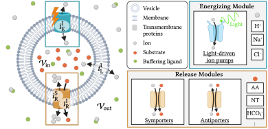
Figure 1. General system model for the proposed ND. The variables $i^{\mathrm{I}}_{\mathrm{E}}$, $i^{\mathrm{I}}_{\mathrm{L}}$, $i^{\mathrm{I}}_{\mathrm{R}}$, and $i^{\mathrm{S}}_{\mathrm{R}}$ denote the the flux of ion $\mathrm{I}$ caused by the energizing module, the leakage flux of $\mathrm{I}$, the flux of $\mathrm{I}$ caused by the release module, and the flux of substrate $\mathrm{S}$ caused by the release module, respectively. The possible flux directions between the intravesicular volume, $\mathcal{V}_{\mathrm{in}}$, and the extravesicular volume, $\mathcal{V}_{\mathrm{out}}$, are indicated by arrows. The complex that the buffering ligand may form with $\mathrm{I}$ is also depicted (complex of green and grey dots). Abbreviations: AA = amino acid, NT = neurotransmitter. Created with BioRender.com.

MC is a burgeoning research area in the field of communication engineering and focuses on the development of communication systems that use molecules as information carriers (Nakano2013, 16). Diverging from conventional electromagnetic (EM) wave–based communication, MC has emerged as a novel paradigm, with the potential to facilitate communication in scenarios where EM wave–based methods face limitations, such as in liquid environments or at nanoscale. Therefore, MC offers numerous revolutionary prospective applications including health monitoring, targeted drug delivery (TDD), or the detection of toxic agents in various environments (Nakano2013, 16). The successful deployment of MC systems largely depends on the development of practically realizable TX and receiver (RX) designs tailored to the envisioned application. The majority of research on TXs in MC is theoretical and often relies on unrealistic assumptions such as perfect controlability of the TX release dynamics or instantaneous release of signaling molecules (Noel2016, 17). Some works, however, consider more realistic TX models. In (Ahmadzadeh2022, 1), a molecule harvesting TX, which is capable of (re-)uptake and release of SMs, was proposed. In (Schaefer2022, 21), the controlled release of SMs by pH-driven membrane permeability switches was considered. Nevertheless, there is a lack of externally controllable TX designs that are applicable for a variety of (possible) SMs. In (Arjmandi2016, 2), the release of ions from a ND via ion channels was considered and, in (Grebenstein2019, 11), an MC testbed was presented that utilized bacteria expressing light-driven ion pumps as TX for the release of protons. This shows that ND-based optically controllable TXs are feasible in practice, and the development of more general and more flexible TX concepts allowing for a variety of possible SMs is promising. The authors of (Arjmandi2016, 2) and (Grebenstein2019, 11) focused on bit transmission as use case for MC, where ions as SMs are sufficient, whereas other applications such as TDD may require more sophisticated SMs and, hence, more sophisticated transport proteins for SM release (Soldner2020, 23). Some experimental work has been conducted on the incorporation of light-driven transport proteins and co-transport proteins into synthetic vesicle membranes (Goers2018, 9, 13), showing that synthetic vesicle-based functionalized NDs are feasible. Additionally, in (Stauffer2021, 24), an ND for filtering out pollutants from natural water sources was proposed using a combination of different types of transmembrane proteins.
In this paper, we introduce a realistic externally controllable TX design based on a vesicular ND that is functionalized for the controlled release of a variety of SMs using two different types of transmembrane proteins. One protein operates as energizing module and powers the second protein, which serves as release module for SMs. The energizing module facilitates the conversion of external light energy supplied by a light-emitting diode (LED) to a chemical concentration gradient using light-driven ion pumps. This gradient then drives the release module which enables the release of SMs using ion/SM co-transporters. Generally, the combination of cooperating energizing and release modules for increased SM versatility, which has not been analyzed in the MC literature yet, diversifies the range of future applications of ND-based TXs. Our proposed design potentially enables applications, such as TDD, that require controlled release of sophisticated SMs. Furthermore, in-body fluid systems, e.g., the bloodstream, and most chemical experimental systems rely on buffers for stabilization of ion concentrations (Ellison1958, 7). Whilst often disregarded in MC models, we also consider the influence of this realistic environmental effect on the operation of our proposed TX. This paper, thus, develops a comprehensive mathematical model for the proposed ND-based TX design, which also accounts for buffering effects. The main contributions of this work are as follows:

• We propose a modular, externally controllable TX capable of releasing different types of SMs and operating under realistic environmental conditions.

• We develop analytical and numerical models for the proposed TX design, analyze one possible practical realization, and evaluate the impact of several system parameters on its SM release characteristics.

The remainder of this paper is structured as follows. In Section 2, the proposed generic TX design is introduced and a mathematical description as well as possible biological realizations for energizing and release modules are provided. In Section 3, an analytical characterization of the signals of interest is derived. In Section 4, simulation results for the proposed system are presented, and conclusions are drawn in Section 5.

2. System Model

2.1. ND Architecture

Fig. 1 shows the proposed ND including both the energizing and the release module. The ND has a spherical shape and a lipid or polymer membrane, which enables the encapsulation of molecules as cargo in the intravesicular space, $\mathcal{V}_{\mathrm{in}}$. The vesicle membrane is semi-permeable, i.e., it allows the translocation of some molecules between $\mathcal{V}_{\mathrm{in}}$ and the extravesicular space, $\mathcal{V}_{\mathrm{out}}$. The permeability of the membrane to a specific molecule depends on various factors, including the size of the molecule, with smaller sizes corresponding to a higher membrane permeability. The resulting net flux of ion $\mathrm{I}$ in outward direction, also referred to as leakage, at time $t$ is denoted by $i^{\mathrm{I}}_{\mathrm{L}}(t)$. As $\mathrm{S}$ is generally a larger molecule, e.g., an amino acid, for which the membrane typically has a very low permeability (Chakrabarti1992, 4), we assume that there is no $\mathrm{S}$ leakage over the membrane.

The energizing module is an energy conversion unit transforming the energy of photons into an electrochemical potential (i.e., a concentration and/or charge gradient). Therefore, the energizing module, consisting of $n_{\mathrm{P}}\in\mathbb{N}_{0}$ light-driven ion pumping transmembrane proteins, actively transports ions $\mathrm{I}$ over the membrane. Here, $\mathbb{N}_{0}$ denotes the set of non-negative integers. The influx caused by the energizing module is denoted by $i^{\mathrm{I}}_{\mathrm{E}}(t)$. This flux is generally unidirectional, as the direction of the pumps can be controlled during the insertion process in practice (Goers2018, 9). For the energizing module, several naturally occurring light-driven ion pumps emerge as potential realizations, including proton ($\mathrm{H^{+}}$) pumps (such as bacteriorhodopsin (Grebenstein2019, 11) and proteorhodopsin (PR) (Dioumaev2003, 6)), light-driven chloride ($\ce{Cl-}$) pumps (Schobert1982, 22), and light-driven sodium ($\ce{Na+}$) pumps (Soldner2020, 23).

The release module leverages the established ion concentration gradient as energy supply for the transport of the encapsuled substrate $\mathrm{S}$ across the ND membrane via $n_{\mathrm{Sym}}\in\mathbb{N}_{0}$ $\mathrm{I}$/$\mathrm{S}$ co-transporters. Two main groups of co-transporters exist: Symporters transport both molecules $\mathrm{S}$ and $\mathrm{I}$ in the same direction (see bottom left box in Fig. 1), while antiporters act as exchangers, i.e., $\mathrm{S}$ is transported in the opposite direction as $\mathrm{I}$ (see bottom right box in Fig. 1). The outfluxes of $\mathrm{I}$ and $\mathrm{S}$ caused by the release module are denoted by $i^{\mathrm{I}}_{\mathrm{R}}(t)$ and $i^{\mathrm{S}}_{\mathrm{R}}(t)$, respectively. If antiporters are used for the release module, an $\mathrm{I}$ gradient from $\mathcal{V}_{\mathrm{out}}$ to $\mathcal{V}_{\mathrm{in}}$ has to be established, such that $\mathrm{S}$ is transported from $\mathcal{V}_{\mathrm{in}}$ to $\mathcal{V}_{\mathrm{out}}$, i.e., released from the vesicle. However, an $\mathrm{I}$ concentration gradient in the opposite direction is required if symporters are used. Hence, the required insertion direction of the light-driven $\mathrm{I}$ pumps depends on the type of employed co-transporter. For some co-transporters, it has been found that a minimum concentration gradient of $\mathrm{I}$ across the membrane is necessary to facilitate the transport (Nakamura1986, 15). We denote by $\xi$ the corresponding threshold of the gradient of the negative logarithm of the concentrations between $\mathcal{V}_{\mathrm{in}}$ and $\mathcal{V}_{\mathrm{out}}$ (e.g., $\Delta\mathrm{pH}$ for $\mathrm{I}=\mathrm{H^{+}}$). There is a vast number of natural, ion-driven co-transporters capable of transporting complex substrates. Biological examples include $\ce{H+}$/amino acid symporters or $\ce{Na+}$/amino acid symporters (Foltz2005, 8, 20), $\ce{Na+}$/neurotransmitter symporters (Soldner2020, 23), and $\ce{Cl-}$/bicarbonate antiporters (Reithmeier2016, 18). The choice of the specific energizing and release modules depends on the type of $\mathrm{I}$ that is available, as both the light-driven pumps and co-transporters need to be able to transport it. Whilst there are a number of possible combinations of energizing and release modules, the practical realization of inserting these transport proteins into the vesicle membrane may become challenging and many co-transporters lack a formal kinetic characterization. Thus, for the system analysis and the simulations, we will concentrate on proteins that have already been successfully inserted into synthetic vesicle membranes and for which the transport kinetics are known.

2.2. Modeling Assumptions

For the sake of mathematical tractability, we now make the following assumptions.

• The solution is well-stirred and the total number of ions, $N^{\mathrm{I}}$, and substrate molecules, $N^{\mathrm{S}}$, are known. We assume that the ion and the substrate concentrations are uniform in both $\mathcal{V}_{\mathrm{in}}$ and $\mathcal{V}_{\mathrm{out}}$, as the diffusion of $\mathrm{I}$ and $\mathrm{S}$ is fast in comparison to their transport over the membrane.

• The light signal emitted by the LED, $l(t)$, is binary, i.e., $l(t)\in\{0,1\}$ for all times $t$. Here, $l(t)=1$ indicates that the LED is turned on, and $l(t)=0$ means that the LED is turned off.

• The buffer molecules only interact with $\mathrm{I}$ as they have a low affinity to other molecules.

2.3. System of ODEs Modeling the ND Kinetics

Using assumptions (A1)–(A3), the fluxes of $\mathrm{I}$ and $\mathrm{S}$ caused by the energizing module (comprising $n_{\mathrm{P}}$ pumps) and release module (comprising $n_{\mathrm{Sym}}$ co-transporters), and the leakage (see Fig. 1) can be used to set up a system of coupled ordinary differential equations describing the system kinetics for the proposed TX design as follows

(1) $$V_{\mathrm{in}}\frac{\mathrm{d}C^{\mathrm{I}}_{\mathrm{in}}(t)}{\mathrm{d}t} =i^{\mathrm{I}}_{\mathrm{E}}(t)-i^{\mathrm{I}}_{\mathrm{L}}(t)-i^{\mathrm{I}}_{\mathrm{R}}(t,C^{\mathrm{S}}_{\mathrm{in}}(t)),$$

(2) $$V_{\mathrm{in}}\frac{\mathrm{d}C^{\mathrm{S}}_{\mathrm{in}}(t)}{\mathrm{d}t} =-i^{\mathrm{S}}_{\mathrm{R}}(t,C^{\mathrm{I}}_{\mathrm{in}}(t)),$$

where $V_{\mathrm{in}}$, $C^{\mathrm{I}}_{\mathrm{in}}(t)$, $i^{\mathrm{I}}_{\mathrm{E}}(t)$, $i^{\mathrm{I}}_{\mathrm{R}}(t)$, $C^{\mathrm{S}}_{\mathrm{in}}(t)$, and $i^{\mathrm{S}}_{\mathrm{R}}(t)$ are the volume of $\mathcal{V}_{\mathrm{in}}$ in ${\mathrm{m}}^{3}$, intravesicular concentration of $\mathrm{I}$ in $\mathrm{mol}\text{\,}{\mathrm{m}}^{-3}$, the influx of $\mathrm{I}$ caused by the energizing module, the outflux of $\mathrm{I}$ caused by the release module, the intravesicular concentration of $\mathrm{S}$ in $\mathrm{mol}\text{\,}{\mathrm{m}}^{-3}$, and the outflux of $\mathrm{S}$ caused by the release module, respectively. All fluxes are measured in $\mathrm{mol}\text{\,}{\mathrm{s}}^{-1}$. Note that the coupled system of ODEs in (1) and (2) only considers the concentrations in $\mathcal{V}_{\mathrm{in}}$, but is sufficient to characterize the entire system, as $N^{\mathrm{S}}$ and $N^{\mathrm{I}}$ are constant and known. The concentrations in $\mathcal{V}_{\mathrm{out}}$ can thus be derived from those in $\mathcal{V}_{\mathrm{in}}$, i.e., $C^{\mathrm{I}}_{\mathrm{out}}(t)=(N^{\mathrm{I}}-C^{\mathrm{I}}_{\mathrm{in}}(t)V_{\mathrm{in}})/V_{\mathrm{out}}$ and $C^{\mathrm{S}}_{\mathrm{out}}(t)=(N^{\mathrm{S}}-C^{\mathrm{S}}_{\mathrm{in}}(t)V_{\mathrm{in}})/V_{\mathrm{out}}$, where $V_{\mathrm{out}}$ is the volume of $\mathcal{V}_{\mathrm{out}}$ in ${\mathrm{m}}^{3}$.

The system of ODEs (1) and (2) does not consider any buffering effects, yet. However, as metal ion or pH buffers are used in most experimental environments and are present, e.g., in in-body fluids, their effect should be taken into account. We consider the following reversible reaction between $\mathrm{I}$ and a buffering ligand $\mathrm{L}$

(3)

where $\mathrm{I}\mathrm{L}$, $k_{\mathrm{-}}$, and $k_{\mathrm{+}}$ are the complex formed by the ion and the ligand, the unbinding rate constant of $\mathrm{I}$ from $\mathrm{L}$, and the binding rate constant of $\mathrm{I}$ to $\mathrm{L}$, respectively. The dissociation constant of the ligand in equilibrium is $k_{\mathrm{D}}=k_{\mathrm{-}}/k_{\mathrm{+}}$ in $\mathrm{mol}\text{\,}{\mathrm{m}}^{-3}$. Using the mass action law, we obtain for the concentration of $\mathrm{I}$ in the buffered system

(4) $$-\log(C^{\mathrm{I}})=-\log(k_{\mathrm{D}})+\log(C^{\mathrm{L}})-\log(C^{\mathrm{I}\mathrm{L}}),$$

where $C^{\mathrm{X}}$ denotes the concentration of molecule $\mathrm{X}$. Note that for $\mathrm{I}\;\hat{=}\;\mathrm{H^{+}}$ the ligand $\mathrm{L}$ would be a base and $-\log(C^{\mathrm{H^{+}}})=\mathrm{pH}$. In this case, (4) specializes to the well-known Henderson-Hasselbalch equation (Ellison1958, 7). Generally, the buffer molarity is given by $C_{0}=C^{\mathrm{I}\mathrm{L}}+C^{\mathrm{I}}$ and remains constant. Thus, in equilibrium and at a given $\mathrm{I}$ concentration, $C^{\mathrm{I}}$ and $C^{\mathrm{I}\mathrm{L}}$ can be deduced from (4). We do not explicitly model the concentration of the buffer molecules in our system of ODEs, as the required extension is not straightforward. Instead, in the simulations, (4) will serve as the ground truth for the buffering effect, while we approximate the effect for the analytical models (see Section 3.6).

3. System Analysis and Analytical Models

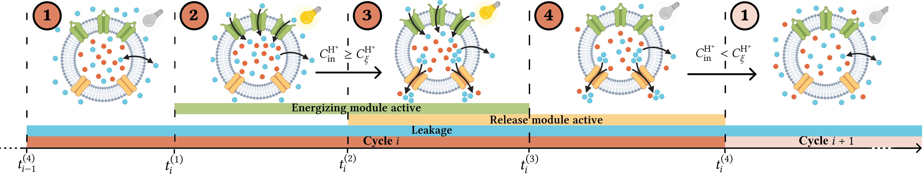
Figure 2. A typical illumination cycle for a vesicle with $\smash{n_{\mathrm{P}}=3}$ and $\smash{n_{\mathrm{Sym}}=2}$ comprising four different cycle phases. The times $\smash{t^{(1)}_{i}}$, $\smash{t^{(2)}_{i}}$, $\smash{t^{(3)}_{i}}$, and $\smash{t^{(4)}_{i}}$ mark the transitions between two adjacent cycle phases. Here, $\smash{C^{\mathrm{H^{+}}}_{\mathrm{in,}\xi}}$ indicates the intravesicular $\smash{\mathrm{H^{+}}}$ concentration, $\smash{C^{\mathrm{H^{+}}}_{\mathrm{in}}(t)}$, at which the symporters become active. Parts of the image were created with BioRender.com.

This section investigates one realization of the proposed ND using a light-driven $\mathrm{H^{+}}$ pump (such as PR (Dioumaev2003, 6)) and an $\mathrm{H^{+}}$ symporter (e.g., PAT1 (Foltz2005, 8)) as energizing and release modules, respectively. Hence, $\mathrm{I}\;\hat{=}\;\mathrm{H^{+}}$ in the rest of this paper. Consequently, the mathematical analysis in this section considers the buffer effect on the $\mathrm{H^{+}}$ concentration. As the use of light-driven $\mathrm{H^{+}}$ pumps allows for a variety of possible release modules and, hence, different $\mathrm{S}$ (e.g., amino acids or neurotransmitters), we continue to consider $\mathrm{S}$ as a generic molecule.

3.1. Functionality of the ND

To discuss the functionality of the proposed ND in detail, it is helpful to examine its behavior upon different external and internal stimuli. Hence, we consider the different states of the ND during one illumination cycle (shown in Fig. 2). A cycle consists of four different phases, which are defined as the time periods during which a certain combination of system components (energizing module, release module, and leakage) are active. The intravesicular $\mathrm{H^{+}}$ threshold concentration for the start of the symport is denoted as $C^{\mathrm{H^{+}}}_{\mathrm{in,}\xi}$ and can be inferred from the pH difference, $\Delta\mathrm{pH}$, threshold $\xi$, and the initial $\mathrm{H^{+}}$ concentrations in $\mathcal{V}_{\mathrm{in}}$ and $\mathcal{V}_{\mathrm{out}}$. As the external light signal $l(t)\in\{0,1\}$ can be chosen arbitrarily and usually consists of multiple illumination cycles, variable $i\in\mathbb{N}_{0}$ is used to index the cycles. Variables $t^{(j)}_{i}$ for $j\in\{1,2,3,4\}$ denote the end times of phase $j$ in cycle $i$, as shown on the axis in Fig. 2. Typically, the sequence of phases during a cycle $i$ is as follows.

1. Leakage: During the first cycle phase the ND is not illuminated and both types of transport proteins are inactive, i.e., only the leakage influences the $\mathrm{H^{+}}$ flux ($i^{\mathrm{H^{+}}}_{\mathrm{L}}(t)\geq 0$).

2. Energizing module and leakage: When the illumination of the system by the external light source starts at $t^{(1)}_{i}$, the pumps start transporting $\mathrm{H^{+}}$ ($i^{\mathrm{H^{+}}}_{\mathrm{E}}(t)>0$). Simultaneously, the increasing pH difference between $\mathcal{V}_{\mathrm{out}}$ and $\mathcal{V}_{\mathrm{in}}$ leads to a larger leakage outflux of $\mathrm{H^{+}}$ ($i^{\mathrm{H^{+}}}_{\mathrm{L}}(t)>0$).

3. Energizing and release modules, and leakage: When the threshold concentration for symporter activity within the vesicle, $C^{\mathrm{H^{+}}}_{\mathrm{in,}\xi}$, is reached at time $t^{(2)}_{i}$, the symporters become active. The symporters cause an additional outflux of $\mathrm{H^{+}}$ and an outward transport of $\mathrm{S}$ ($i^{\mathrm{H^{+}}}_{\mathrm{R}}(t)>0,i^{\mathrm{S}}_{\mathrm{R}}(t)>0,i^{\mathrm{H^{+}}}_{\mathrm{E}}(t)>0,i^{\mathrm{H^{+}}}_{\mathrm{L}}(t)>0$).

4. Release module and leakage: When the illumination ends at time $t^{(3)}_{i}$, but the intravesicular $\mathrm{H^{+}}$ concentration $C^{\mathrm{H^{+}}}_{\mathrm{in}}(t)$ is still above the symport threshold $C^{\mathrm{H^{+}}}_{\mathrm{in,}\xi}$, the symporters remain active while the pumps stop transporting $\mathrm{H^{+}}$. During this cycle phase, both the symporters and the leakage cause $\mathrm{H^{+}}$ outflux and $\mathrm{S}$ is transported outwards ($i^{\mathrm{H^{+}}}_{\mathrm{R}}(t)>0,i^{\mathrm{S}}_{\mathrm{R}}(t)>0,i^{\mathrm{H^{+}}}_{\mathrm{L}}(t)>0$). When $C^{\mathrm{H^{+}}}_{\mathrm{in}}(t)$ falls below the threshold $C^{\mathrm{H^{+}}}_{\mathrm{in,}\xi}$ at time $t^{(4)}_{i}$, cycle $i$ ends and the next cycle $i+1$ starts.

Note that we assume $t^{(4)}_{0}=0$, i.e., the first cycle ($i=1$) starts at $t=0$. While $t^{(1)}_{i}$ and $t^{(3)}_{i}$ depend on $l(t)$, which can be chosen arbitarily, the symport start and end times, $t^{(2)}_{i}$ and $t^{(4)}_{i}$, depend on the $\mathrm{H^{+}}$ concentrations and, thus, have to be calculated from $C^{\mathrm{H^{+}}}_{\mathrm{in}}(t)$, as shown in Section 3.5. Note that by definition during an illumination cycle the light source turns on and off exactly once. Generally, different types of illumination cycles can occur, e.g., if the symporters do not become active during illumination. This means (P1)–(P4) do not necessarily occur in each cycle. However, due to space constraints, we leave the extension of our model to other cycle types for future work. Note that indexing by $i$ is required for the time variables limiting the cycle phases, but can be omitted for the fluxes and concentrations, which are defined for absolute time. This is possible because the time variables for new cycles are monotonically increasing (see Fig. 2).

3.2. Proton and Substrate Fluxes

To derive solutions to (1) and (2) in Sections 3.3 and 3.4, a mathematical model for the $\mathrm{H^{+}}$ and $\mathrm{S}$ fluxes caused by the system components is required. We assume that the light-driven proton pumps always operate at maximum effective rate as long as enough $\mathrm{H^{+}}$ is available in $\mathcal{V}_{\mathrm{out}}$ during illumination. As the transport process of $\mathrm{H^{+}}$ by light-driven pumps is rate-limited by one reaction, this assumption is well-justified (Bamann2014, 3). Consequently, the $\mathrm{H^{+}}$ flux in $\mathrm{mol}\text{\,}{\mathrm{s}}^{-1}$ caused by the energizing module, $i^{\mathrm{H^{+}}}_{\mathrm{E}}(t)$, is obtained as

(5) $$i^{\mathrm{H^{+}}}_{\mathrm{E}}(t)=\frac{C^{\mathrm{H^{+}}}_{\mathrm{out}}(t)}{C^{\mathrm{H+}}_{\mathrm{out,0}}}\gamma_{\mathrm{P}}\mathds{1}_{\{1\}}(l(t)),$$

where $C^{\mathrm{H+}}_{\mathrm{out,0}}$, $\gamma_{\mathrm{P}}$, and $\mathds{1}_{\mathcal{X}}(x)$ are the initial $\mathrm{H^{+}}$ concentration in $\mathcal{V}_{\mathrm{out}}$, the effective rate constant of $\mathrm{H^{+}}$ caused by $n_{\mathrm{P}}$ proton pumps, and the indicator function, i.e., $\mathds{1}_{\mathcal{X}}(x)=1$, if $x\in\mathcal{X}$, and $\mathds{1}_{\mathcal{X}}(x)=0$, otherwise, respectively. The effective pumping rate of one vesicle, $\gamma_{\mathrm{P}}=\hat{\gamma}_{\mathrm{P}}n_{\mathrm{P}}/\mathrm{N}_{\mathrm{A}}$ in $\mathrm{mol}\text{\,}{\mathrm{s}}^{-1}$, depends on the effective pumping rate of one proton pump $\hat{\gamma}_{\mathrm{P}}$ in ${\mathrm{s}}^{-1}$, the number of pumps $n_{\mathrm{P}}$, and the Avogadro constant $\mathrm{N}_{\mathrm{A}}=$6.022\text{\times}{10}^{23}\text{\,}{\mathrm{mol}}^{-1}$$.

We assume that the symporters are only active if the intravesicular $\mathrm{H^{+}}$ concentration, $C^{\mathrm{H^{+}}}_{\mathrm{in}}(t)$, crosses the threshold $C^{\mathrm{H^{+}}}_{\mathrm{in,}\xi}$, based on the co-transporter kinetics described in the literature (Nakamura1986, 15, 8). The associated $\mathrm{S}$ and $\mathrm{H^{+}}$ fluxes can be described as follows

(6)

where $\gamma^{\mathrm{S}}_{\mathrm{Sym}}$, $K_{\mathrm{m}}$, and $\nu_{\mathrm{Sym}}\in\mathbb{Q}$ are the effective $\mathrm{S}$ symport rate constant of one vesicle, the Michaelis-Menten constant in $\mathrm{mol}\text{\,}{\mathrm{m}}^{-3}$, and the ratio of $\mathrm{H^{+}}$ to $\mathrm{S}$ molecules that are co-transported by the symporters, respectively. Here $\mathbb{Q}$ denotes the set of rational numbers. As $\nu_{\mathrm{Sym}}$ is fixed and depends on the molecular structure of the co-transporter, the $\mathrm{H^{+}}$ and $\mathrm{S}$ fluxes caused by the protein can simply be deduced from one another by multiplication or division by $\nu_{\mathrm{Sym}}$. The effective symport rate of one vesicle is given by $\gamma^{\mathrm{S}}_{\mathrm{Sym}}=\hat{\gamma}^{\mathrm{S}}_{\mathrm{Sym}}n_{\mathrm{Sym}}/\mathrm{N}_{\mathrm{A}}$ in $\mathrm{mol}\text{\,}{\mathrm{s}}^{-1}$, where $\hat{\gamma}^{\mathrm{S}}_{\mathrm{Sym}}$ is the effective $\mathrm{S}$ transport rate constant of one symporter in ${\mathrm{s}}^{-1}$ and $n_{\mathrm{Sym}}$ is the number of symporters in the vesicle membrane. The symport threshold concentration is $C^{\mathrm{H^{+}}}_{\mathrm{in,}\xi}=N^{\mathrm{H^{+}}}/(V_{\mathrm{out}}10^{-\xi}+V_{\mathrm{in}})$ and is obtained from the initial system pH and the $\Delta\mathrm{pH}$ threshold, $\xi$, between $\mathcal{V}_{\mathrm{in}}$ and $\mathcal{V}_{\mathrm{out}}$ needed for the start of the symport (Nakamura1986, 15). Note that the symporters are naturally only active as long as $C^{\mathrm{S}}_{\mathrm{in}}(t)>0$, i.e., as long as $\mathrm{S}$ is available. Hence, the symporters become inactive when the vesicle has released all of its cargo. This state is referred to as substrate depletion.

Lastly, the $\mathrm{H^{+}}$ flux caused by leakage of $\mathrm{H^{+}}$ over the vesicle membrane is obtained as follows

(7) $$i^{\mathrm{H^{+}}}_{\mathrm{L}}(t)=\gamma_{\mathrm{L}}\left(C^{\mathrm{H^{+}}}_{\mathrm{in}}(t)-C^{\mathrm{H^{+}}}_{\mathrm{out}}(t)\right),$$

where $\gamma_{\mathrm{L}}=\hat{\gamma}_{\mathrm{L}}A_{\mathrm{ves}}$ is the membrane permeability to $\mathrm{H^{+}}$ in ${\mathrm{m}}^{3}\text{\,}{\mathrm{s}}^{-1}$. Here, $\hat{\gamma}_{\mathrm{L}}$ is the proton diffusion rate over the vesicle membrane in $\mathrm{m}\text{\,}{\mathrm{s}}^{-1}$ and $A_{\mathrm{ves}}$ is the outer surface area of the vesicle in ${\mathrm{m}}^{2}$. Note that the leakage flux scales with the $\mathrm{H^{+}}$ concentration gradient between $\mathcal{V}_{\mathrm{in}}$ and $\mathcal{V}_{\mathrm{out}}$.

3.3. Exact Analytical Solution

For the analytical solution, the ODEs (1) and (2) are considered separately for each cycle phase shown in Fig. 2. We introduce the variable $\tau_{0}(t)$ to indicate the starting time of the current cycle phase

(8) $$\tau_{0}(t)=\max_{i,j}\big{\{}t^{(j)}_{i}\left|\right.t^{(j)}_{i}<t\big{\}},\quad\forall j\in\{1,2,3,4\}.$$

Additionally, we define $f(t):=C^{\mathrm{S}}_{\mathrm{in},0}(t)/K_{\mathrm{m}}\,\mathrm{exp}([C^{\mathrm{S}}_{\mathrm{in},0}(t)-\gamma^{\mathrm{S}}_{\mathrm{Sym}}/V_{\mathrm{in}}(t-\tau_{0}(t))]/K_{\mathrm{m}})$, where $C^{\mathrm{S}}_{\mathrm{in},0}(t)=C^{\mathrm{S}}_{\mathrm{in}}(\tau_{0}(t))$ denotes the initial intravesicular $\mathrm{S}$ concentration of the current cycle phase. Note that $C^{\mathrm{S}}_{\mathrm{in,0}}:=C^{\mathrm{S}}_{\mathrm{in}}(0)$ denotes the initial intravesicular $\mathrm{S}$ concentration in the system. Moreover, to be able to express $C^{\mathrm{S}}_{\mathrm{in}}(t)$ and $C^{\mathrm{H^{+}}}_{\mathrm{in}}(t)$ in the following proposition in a compact manner, we introduce the cycle phase–dependent variables $a$ and $b$

(9) $$a=j^{a}_{\mathrm{L}}+j^{a}_{\mathrm{P}}\mathds{1}_{\{t^{(1)}_{i},t^{(2)}_{i}\}}(\tau_{0}(t)),\quad b=j^{b}_{\mathrm{L}}+j^{b}_{\mathrm{P}}\mathds{1}_{\{t^{(1)}_{i},t^{(2)}_{i}\}}(\tau_{0}(t))$$

with auxiliary variables $j^{a}_{\mathrm{L}}=\gamma_{\mathrm{L}}(V_{\mathrm{in}}^{-1}+V_{\mathrm{out}}^{-1})$, $j^{a}_{\mathrm{P}}=\gamma_{\mathrm{P}}/(V_{\mathrm{out}}C^{\mathrm{H+}}_{\mathrm{out,0}})$, $j^{b}_{\mathrm{L}}=-\gamma_{\mathrm{L}}N^{\mathrm{H^{+}}}/(V_{\mathrm{out}}V_{\mathrm{in}})$, and $j^{b}_{\mathrm{P}}=j^{a}_{\mathrm{P}}N^{\mathrm{H^{+}}}/V_{\mathrm{in}}$.

Proposition 1.

The intravesicular $\mathrm{S}$ concentration, $C^{\mathrm{S}}_{\mathrm{in}}(t)$, is obtained as follows

(10) $$C^{\mathrm{S}}_{\mathrm{in}}(t)=\begin{cases}K_{\mathrm{m}}\mathrm{W}\left\{f(t)\right\},&\text{if }t^{(2)}_{i}<t\leq t^{(4)}_{i},\\ C^{\mathrm{S}}_{\mathrm{in},0}(t),&\text{if }t\leq t^{(2)}_{i}\text{ or }t^{(4)}_{i}<t,\end{cases}$$

where $\mathrm{W}\left\{\cdot\right\}$ denotes the Lambert W–function, defined by
${\mathrm{W}\left\{x\right\}\mathrm{exp}(\mathrm{W}\left\{x\right\})=x}$. $C^{\mathrm{H^{+}}}_{\mathrm{in}}(t)$, the intravesicular $\mathrm{H^{+}}$ concentration is obtained as follows

(11) $$C^{\mathrm{H^{+}}}_{\mathrm{in}}(t)=\left[C^{\mathrm{H^{+}}}_{\mathrm{in},0}(t)-\alpha(\tau_{0}(t))+\alpha(t)\right]\mathrm{e}^{-a(t-\tau_{0}(t))},$$

where $C^{\mathrm{H^{+}}}_{\mathrm{in},0}(t)=C^{\mathrm{H^{+}}}_{\mathrm{in}}(\tau_{0}(t))$ is the initial intravesicular $\mathrm{H^{+}}$ concentration of the current cycle phase and

(12)

∎

Proof.

Due to space limitations, we provide only a sketch of the proof. We obtain (10) by inserting (6) into (2) and solving for $C^{\mathrm{S}}_{\mathrm{in}}(t)$. For a detailed derivation of the solution of the integral of a Michaelis-Menten term, we refer the reader to Section 2 of (Goudar1999, 10). We obtain (11) by inserting (10) and (5)–(7) into (1), resulting in

(13) $$\frac{\mathrm{d}C^{\mathrm{H^{+}}}_{\mathrm{in}}(t)}{\mathrm{d}t}=-aC^{\mathrm{H^{+}}}_{\mathrm{in}}(t)+b-\mathds{1}_{[C^{\mathrm{H^{+}}}_{\mathrm{in,}\xi},\infty)}(C^{\mathrm{H^{+}}}_{\mathrm{in}}(t))\frac{\gamma^{\mathrm{H^{+}}}_{\mathrm{Sym}}}{V_{\mathrm{in}}}\frac{\mathrm{W}\left\{f(t)\right\}}{\mathrm{W}\left\{f(t)\right\}+1}.$$

Solving this inhomogeneous ODE by variation of the constant yields the time-variant integration constant $\alpha(t)$ (see (12)). ∎

Note that the integral in (12) cannot be solved in closed form and has to be computed numerically.

3.4. Closed-Form Approximation

To obtain a computationally efficient and tractable approximate analytical solution for $C^{\mathrm{H^{+}}}_{\mathrm{in}}(t)$ and $C^{\mathrm{S}}_{\mathrm{in}}(t)$ during all cycle phases that circumvents the numerical integration of $\alpha(t)$ in (12), we approximate the Michaelis-Menten term in (6) by linearization as follows

(14) $$i^{\mathrm{S}}_{\mathrm{R}}(t)\approx\gamma^{\mathrm{S}}_{\mathrm{Sym}}\mathds{1}_{\mathbb{R}^{+}}(C^{\mathrm{S}}_{\mathrm{in}}(t)),\quad i^{\mathrm{H^{+}}}_{\mathrm{R}}(t)=\nu_{\mathrm{Sym}}i^{\mathrm{S}}_{\mathrm{R}}(t),$$

where $\mathbb{R}^{+}$ denotes the set of positive real numbers. Approximation (14) is justified for long time spans if $C^{\mathrm{S}}_{\mathrm{in,0}}\gg K_{\mathrm{m}}$ and implies that the symporters operate with maximum rate as long as $\mathrm{S}$ is available and stop transporting as soon as $C^{\mathrm{S}}_{\mathrm{in}}(t)=0$. After inserting (14) into (2), it can be shown that (10) simplifies to

(15) $$C^{\mathrm{S}}_{\mathrm{in}}(t)=\begin{cases}C^{\mathrm{S}}_{\mathrm{in},0}(t)-\frac{\gamma^{\mathrm{S}}_{\mathrm{Sym}}(t)}{V_{\mathrm{in}}}\left[t-\tau_{0}(t)\right],&\text{if }t^{(2)}_{i}<t\leq t^{(4)}_{i},\\ C^{\mathrm{S}}_{\mathrm{in},0}(t),&\text{if }t^{(4)}_{i-1}<t\leq t^{(2)}_{i},\end{cases}$$

where $\gamma^{\mathrm{S}}_{\mathrm{Sym}}(t)=\gamma^{\mathrm{S}}_{\mathrm{Sym}}\mathds{1}_{\mathbb{R}^{+}}(C^{\mathrm{S}}_{\mathrm{in}}(t))$ is the time-dependent transport rate obtained from (14).

Moreover, it can be shown that (11) simplifies to

(16) $$C^{\mathrm{H^{+}}}_{\mathrm{in}}(t)=a^{-1}b^{\prime}-\left[C^{\mathrm{H^{+}}}_{\mathrm{in},0}(t)-a^{-1}b^{\prime}\right]\mathrm{e}^{-a(t-\tau_{0}(t))},$$

where $b^{\prime}=b+j^{b}_{\mathrm{Sym}}(t)\mathds{1}_{\{t^{(2)}_{i},t^{(3)}_{i}\}}(\tau_{0}(t))$ with $j^{b}_{\mathrm{Sym}}(t)=-\gamma^{\mathrm{H^{+}}}_{\mathrm{Sym}}(t)/V_{\mathrm{in}}$. In contrast to (10) and (11), the closed-form approximations (15) and (16) can be used to determine signal parameters such as the symporter start and end times and the time of $\mathrm{S}$ depletion.

The validity of the analytical solutions (10) and (11) and the closed-form approximations (15) and (16) will be verified by comparison to a numerical solution of ODEs (1) and (2) using the finite difference method (FDM) (Grossmann2007, 12). For the results presented in Section 4, we will consider the FDM results as the ground truth.

3.5. Calculation of Cycle Phase Limits

As mentioned in Section 3.1 and shown in Fig. 2, the limits of the phases in cycle $i$ are defined by $t^{(j)}_{i}$ for $j\in\{1,2,3,4\}$. The times $t^{(1)}_{i}$ and $t^{(3)}_{i}$ for the start and the end of the illumination can be chosen arbitrarily. In contrast, the symport start and end times, $t^{(2)}_{i}$ and $t^{(4)}_{i}$, have to be calculated from the preceding cycle phases, i.e., phases (P2) and (P4), respectively. As (11) is not invertible, $t^{(2)}_{i}$ and $t^{(4)}_{i}$ cannot be inferred from the exact solution. In contrast, the closed-form approximation (16) can be inverted for all cycle phases, leading to

(17)

for $x\in\{2,4\}$. Note that the values obtained from (17) are only valid for illumination cycles exhibiting the same sequence of phases as the one considered in Fig. 2.

3.6. Influence of Buffer

We assume that the system is immersed in a buffer suspension (see Section 2.3) with total buffer molarity $C_{0}$ in both volumes $\mathcal{V}_{\mathrm{in}}$ and $\mathcal{V}_{\mathrm{out}}$. Equation (4) can be used to calculate the pH of a monoprotic buffer using the concentration of acid and base molecules and, thus, allows for an explicit buffer modeling. It can be incorporated into the numerical FDM solution.

However, (4) is not amenable to analytical solutions as it leads to an intractable system of ODEs. Thus, we approximate the effect of the buffer suspension as an attenuation of the $\mathrm{H^{+}}$ flux from one volume to another. This approach simply scales the flux rates of $\mathrm{H^{+}}$, i.e., $\gamma_{\mathrm{L}}$, $\gamma_{\mathrm{P}}$, and $\gamma^{\mathrm{H^{+}}}_{\mathrm{Sym}}$, by a factor $\vartheta_{\mathrm{buf}}(t)=k_{\mathrm{D}}C_{0}(C^{\mathrm{H^{+}}}_{\mathrm{in}}(t)+k_{\mathrm{D}})^{-2}$ (Zifarelli2008, 26). This attenuation factor depends on the inner $\mathrm{H^{+}}$ concentration $C^{\mathrm{H^{+}}}_{\mathrm{in}}(t)$ and therefore varies over time. The use of this time-variant attenuation factor thus leads to a system of non-linear ODEs. To avoid this, we assume that during each cycle phase the attenuation factor remains constant and can be computed using the initial intravesicular $\mathrm{H^{+}}$ concentration of the cycle phase, $C^{\mathrm{H^{+}}}_{\mathrm{in},0}(t)=C^{\mathrm{H^{+}}}_{\mathrm{in}}(\tau_{0}(t))$, i.e.,

(18) $$\vartheta_{\mathrm{buf}}(\tau_{0}(t))\approx k_{\mathrm{D}}C_{0}(C^{\mathrm{H^{+}}}_{\mathrm{in}}(\tau_{0}(t))+k_{\mathrm{D}})^{-2}.$$

Note that only values $\vartheta_{\mathrm{buf}}(\tau_{0}(t))>1$ are valid as other values correspond to an unbuffered scenario, which does not require flux attenuation. Scaling the $\mathrm{H^{+}}$ fluxes in (1) and (2) with (18) leads to a system of ODEs with a tractable solution for all cycle phases. In fact, the obtained solution is similar to (16) and simply uses rescaled auxiliary variables $j^{x*}_{Y}=j^{x}_{Y}\vartheta_{\mathrm{buf}}(\tau_{0}(t))^{-1}$ for $x\in\{a,b\}$ and $y\in\{\mathrm{L},\mathrm{P},\mathrm{Sym}\}$. In our simulations, we will validate this approximation of the buffer effect in (18) by comparison to the explicit buffer modeling using numerical FDM.

4. Simulation Results

In this section, the results obtained for the exact analytical solution (10) and (11) and the closed-form approximation (15) and (16) describing the proposed ND are presented and compared to the numerical results obtained with FDM. First, we investigate the impact of the buffer molarity on the dynamics of the energizing module. Then, the functionality of the entire ND is examined with varying ratios of the numbers of pumps and symporters. As the transport rate of proteins cannot be changed straightforwardly, the numbers of pumps and symporters in the vesicle membrane are important design parameters as they directly scale the fluxes of $\mathrm{I}$ and $\mathrm{S}$ (see (5) and (6)). Lastly, the influence of different transport rates of symporters (which could correspond to different symporter realizations) and membrane permeabilities on the symport duration for different illumination durations is discussed. All simulations are conducted using the default parameters in Table 1 if not specified otherwise. These default values are chosen to be in line with experimental data if available. The time step $\mathrm{\Delta}t$ is relevant for the numerical FDM baseline, which requires time discretization.

Table 1. Default parameters for the simulations.

Parameter	Value		Reference
$\mathrm{\Delta}t$	$1\text{\times}{10}^{-2}$	$\mathrm{s}$
$C^{\mathrm{S}}_{\mathrm{in,0}}$	$300$	$\mathrm{mol}\text{\,}{\mathrm{m}}^{-3}$
$C_{0}$	$20$	$\mathrm{mol}\text{\,}{\mathrm{m}}^{-3}$
$k_{\mathrm{D}}$	$6.2\text{\times}{10}^{-5}$	$\mathrm{mol}\text{\,}{\mathrm{m}}^{-3}$	(Ellison1958, 7)
$d_{\mathrm{in}}$	$87$	$\mathrm{nm}$	(Rideau2018, 19)
$d_{\mathrm{mem}}$	$14$	$\mathrm{nm}$	(Rideau2018, 19)
$V_{\mathrm{out}}$	$1\text{\times}{10}^{-6}$	${\mathrm{m}}^{3}$	(Goers2018, 9)
$C^{\mathrm{H^{+}}}_{\mathrm{in,0}}$, $C^{\mathrm{H+}}_{\mathrm{out,0}}$	$3.98\text{\times}{10}^{-5}$	$\mathrm{mol}\text{\,}{\mathrm{m}}^{-3}$

Parameter	Value		Reference
$K_{\mathrm{m}}$	$1.3\text{\times}{10}^{-2}$	$\mathrm{mol}\text{\,}{\mathrm{m}}^{-3}$	(Levy1998, 14)
$\nu_{\mathrm{Sym}}$	$3$		(Ryan2009, 20)
$\hat{\gamma}^{\mathrm{S}}_{\mathrm{Sym}}$	$0.006$	${\mathrm{s}}^{-1}$	(Tubbe1992, 25)
$n_{\mathrm{Sym}}$	$30$		(Goers2018, 9)
$\gamma_{\mathrm{L}}$	$3\text{\times}{10}^{-6}$	$\mathrm{m}\text{\,}{\mathrm{s}}^{-1}$	(Deamer1987, 5)
$\hat{\gamma}_{\mathrm{P}}$	$0.1$	${\mathrm{s}}^{-1}$	(Dioumaev2003, 6)
$n_{\mathrm{P}}$	$40$		(Goers2018, 9)
$\xi$	0.015

4.1. Energizing Module

In order to assess the functionality of the proposed $\mathrm{H^{+}}$-based energizing module under varying experimental conditions, we consider an ND without release module, i.e., $n_{\mathrm{Sym}}=0$, for different buffer molarities $C_{0}$. Fig. 3 shows $C^{\mathrm{H^{+}}}_{\mathrm{in}}(t)$ as obtained from the exact analytical solution (11) (green), the approximate solution (16) (orange), and the numerical FDM solution as baseline (blue). The results were obtained for $600\text{\,}\mathrm{s}$ of continuous illumination followed by an equally long period without light excitation. We note that the general signal shapes are in agreement with experimental data from the literature employing a similar set up using light-driven $\mathrm{H^{+}}$ pumps (compare Fig. 3 with Fig. 3 in (Harder2024, 13)). In both our simulations and the experimental measurements, illumination causes an exponentially-decaying increase in $C^{\mathrm{H^{+}}}_{\mathrm{in}}(t)$ (i.e., a decrease in the intravesicular pH) and dark phases cause a return to the initial value of $C^{\mathrm{H^{+}}}_{\mathrm{in}}(t)$. This suggests that our developed system model successfully captures the behavior of the envisioned ND. Fig. 3 highlights the importance of modeling the buffer, as the system dynamics of a buffered system ($C_{0}>$0\text{\,}\mathrm{mol}\text{\,}{\mathrm{m}}^{-3}$$) are clearly very different from those of an unbuffered system ($C_{0}=$0\text{\,}\mathrm{mol}\text{\,}{\mathrm{m}}^{-3}$$). We observe that a higher buffer molarity causes a smaller slope of $C^{\mathrm{H^{+}}}_{\mathrm{in}}(t)$ during both the illumination period ($l(t)=1$) and the dark period ($l(t)=0$). As expected, for increasing buffer molarity, the $\mathrm{H^{+}}$ in- and outfluxes are more attenuated and therefore the rate of $\mathrm{H^{+}}$ concentration change is smaller. It is noteworthy that, for all buffer molarities, $C^{\mathrm{H^{+}}}_{\mathrm{in}}(t)$ approaches the same value for long illumination durations. This value is the dynamic equilibrium concentration $C^{\mathrm{H^{+}}}_{\mathrm{in,eq}}$ (black line in Fig. 3), where the influx $i^{\mathrm{H^{+}}}_{\mathrm{E}}(t)$ caused by the pumps is equal to the outflux $i^{\mathrm{H^{+}}}_{\mathrm{L}}(t)$ caused by the leakage. As all $\mathrm{H^{+}}$ molecules entering or leaving $\mathcal{V}_{\mathrm{in}}$ are equally buffered, $C^{\mathrm{H^{+}}}_{\mathrm{in,eq}}$ is unaffected by the buffer molarity. However, as can be seen in Fig. 3, the speed at which the equilibrium is reached changes, e.g., the curve for $C_{0}=$100\text{\,}\mathrm{mol}\text{\,}{\mathrm{m}}^{-3}$$ does not reach $C^{\mathrm{H^{+}}}_{\mathrm{in,eq}}$ for the setting shown in Fig. 3 as the illumination period is too short. Generally, Fig. 3 shows that the analytical solutions are in good agreement with the numerical baseline. Interestingly, the closed-form approximation is very accurate while entailing a much lower computational cost compared to the other solutions. However, when the changes in $C^{\mathrm{H^{+}}}_{\mathrm{in}}(t)$ are large in the buffered scenario, e.g., for low buffer molarities (e.g., $C_{0}=$10\text{\,}\mathrm{mol}\text{\,}{\mathrm{m}}^{-3}$$), there are small deviations between the analytical solutions and the FDM solution in the speed at which $C^{\mathrm{H^{+}}}_{\mathrm{in,eq}}$ is reached. The reason for these deviations is the phase-wise constant attenuation factor $\vartheta_{\mathrm{buf}}(\tau_{0}(t))$ in (18), which becomes erroneous during long illumination periods before $C^{\mathrm{H^{+}}}_{\mathrm{in,eq}}$ is reached and after substantial $\mathrm{H^{+}}$ in- or outflux has caused changes in $C^{\mathrm{H^{+}}}_{\mathrm{in}}(t)$, as $C^{\mathrm{H^{+}}}_{\mathrm{in}}(t)$ is assumed constant in (18). Conclusively, we note that the buffer molarity of the system determines how responsive the energizing module is with respect to changes in the external stimulus. Higher buffer molarities introduce a latency to the stimulus response, while low buffer molarities lead to a more responsive system.

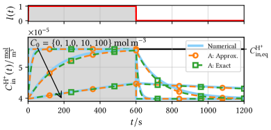
Figure 3. Intravesicular $\mathrm{H^{+}}$ concentration (bottom) for one illumination period without release module, i.e., $n_{\mathrm{Sym}}=0$, and for varying buffer molarities $C_{0}$. Results obtained with FDM (blue), the exact analytical solution (11) (green), and the approximate analytical solution (16) (orange) are shown. The light signal $l(t)$ is plotted on the top. Shaded gray areas indicate times during which $l(t)=1$. The black line shows the $\mathrm{H^{+}}$ concentration, $C^{\mathrm{H^{+}}}_{\mathrm{in,eq}}$, where in- and outflux to/from the vesicle are in equilibrium.

4.2. Energizing and Release Module

Fig. 4 shows $C^{\mathrm{H^{+}}}_{\mathrm{in}}(t)$, $C^{\mathrm{S}}_{\mathrm{out}}(t)$, and the outflux of $\mathrm{S}$ caused by the release module, $i^{\mathrm{S}}_{\mathrm{R}}(t)$, for different ratios of $n_{\mathrm{P}}$ and $n_{\mathrm{Sym}}$ while the total number of membrane proteins $n_{\mathrm{P}}+n_{\mathrm{Sym}}$ remains constant. In comparison to Fig. 3, which showed a scenario without release modules, the slope of $C^{\mathrm{H^{+}}}_{\mathrm{in}}(t)$ decreases when the symporters are active, i.e., for $C^{\mathrm{H^{+}}}_{\mathrm{in}}(t)>C^{\mathrm{H^{+}}}_{\mathrm{in,}\xi}$. Generally, we observe that a smaller number of symporters leads to larger $C^{\mathrm{H^{+}}}_{\mathrm{in}}(t)$ during the illumination phases due to a lower symport-caused $\mathrm{H^{+}}$ outflux. Similarly, the influence of a lower number of symporters is also observable in the smaller slope of $C^{\mathrm{S}}_{\mathrm{out}}(t)$ (see left-hand side of center panel in Fig. 4) or, equivalently, in the lower $i^{\mathrm{S}}_{\mathrm{R}}(t)$ during illumination periods. However, the higher peaks of $C^{\mathrm{H^{+}}}_{\mathrm{in}}(t)$ for smaller $n_{\mathrm{Sym}}$ lead to a longer symport duration, $t^{(4)}_{i}-t^{(2)}_{i}$, in each cycle as shown by the increasing width of the rectangles in $i^{\mathrm{S}}_{\mathrm{R}}(t)$ for decreasing $n_{\mathrm{Sym}}$. These observations lead to the conclusion that a lower number of symporters does not necessarily correlate with an overall lower amount of released $\mathrm{S}$ (which is proportional to the area of the rectangles in $i^{\mathrm{S}}_{\mathrm{R}}(t)$) as a lower outflux rate causes longer symport durations. For the case $n_{\mathrm{P}}/n_{\mathrm{Sym}}=1$, we also observe the effect of substrate depletion in Fig. 4. We have chosen a low $C^{\mathrm{S}}_{\mathrm{in,0}}=$3.14\text{\,}\mathrm{mol}\text{\,}{\mathrm{m}}^{-3}$$ for which substrate depletion takes place at around $t=$6500\text{\,}\mathrm{s}$$. However, in practice, larger $C^{\mathrm{S}}_{\mathrm{in,0}}$ are achievable and should be used to increase the longevity of the ND (see Table 1). For $n_{\mathrm{P}}/n_{\mathrm{Sym}}=4/3$, the substrate is depleted even earlier as evident from the fact that $i^{\mathrm{S}}_{\mathrm{R}}(t)=0$ for all plotted times $t>$6350\text{\,}\mathrm{s}$$ (highlighted in red in Fig. 4). On the other hand, substrate depletion is not reached during the simulation time for $n_{\mathrm{P}}/n_{\mathrm{Sym}}=3/4$. Consequently, the rectangular signal shape of $i^{\mathrm{S}}_{\mathrm{R}}(t)$ can be observed until the end of the simulation. We also note that during substrate depletion, the accuracy of the approximate solution (15) decreases (see mismatch between the blue and orange curves in the bottom panel of Fig. 4 for $n_{\mathrm{P}}=n_{\mathrm{Sym}}$) due to its inability to capture the decrease in the symport rate characteristic for Michaelis-Menten kinetics (see (6) for $C^{\mathrm{S}}_{\mathrm{in}}(t)\ll K_{\mathrm{m}}$). In contrast, the exact analytical solution (11) does reflect the decrease in symport rate during substrate depletion, and the slight deviations from the numerical baseline are attributed to the finite time resolution in the numerical integration for obtaining $\alpha(t)$ in (12). Note that the light signal in Fig. 4 may be interpreted as a modulated transmit signal for concentration shift keying. Since the difference in $i^{\mathrm{S}}_{\mathrm{R}}(t)$ during illumination and dark phases mimics the shape of the optical transmit signal, the resulting signal may be suitable for encoding information. Generally, Fig. 4 shows that the ratio $n_{\mathrm{P}}/n_{\mathrm{Sym}}$ is an important design parameter of the ND. For example, if the envisioned use case of the ND requires a prolonged, sustained release of $\mathrm{S}$ upon illumination (wide rectangles), large $n_{\mathrm{P}}/n_{\mathrm{Sym}}$ should be chosen, while for shorter temporal responses to the external stimuli (narrow rectangles) small $n_{\mathrm{P}}/n_{\mathrm{Sym}}$ are favorable.

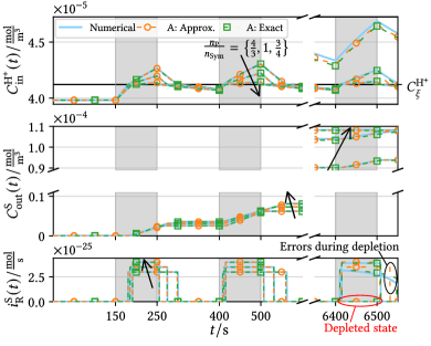
Figure 4. Intravesicular $\mathrm{H^{+}}$ concentration, extravesicular $\mathrm{S}$ concentration, and the outflux of $\mathrm{S}$ caused by the symporters over multiple illumination cycles for varying protein ratios $n_{\mathrm{P}}/n_{\mathrm{Sym}}$ and $C^{\mathrm{S}}_{\mathrm{in,0}}=$3.14\text{\,}\mathrm{mol}\text{\,}{\mathrm{m}}^{-3}$$. The arrows indicate decreasing $n_{\mathrm{P}}/n_{\mathrm{Sym}}$. As in Fig. 3, shaded gray areas indicate times during which $l(t)=1$.

4.3. Estimation of Substrate Release

In order to utilize the proposed ND as TX for synthetic MC for applications such as TDD or bit transmission, it is necessary to design the release of $\mathrm{S}$ adequately in consideration of the limited $\mathrm{S}$ resources inside the vesicle. One important variable in this context is the expected number of released $\mathrm{S}$ (see area of the rectangles in the bottom panel of Fig. 4) in response to a specific illumination duration. Similarly, the expected duration of symport during an illumination cycle is of interest. The closed-form expression (17) proposed in this paper allows for the calculation of the start $t^{(2)}$ and end $t^{(4)}$ times of the symport. To validate the results, we compare the obtained values with the numerically simulated symport duration. The top panel of Fig. 5 shows the symport duration, $t^{(4)}-t^{(2)}$, and the bottom panel shows the final extravesicular $\mathrm{S}$ concentration for varying $\hat{\gamma}_{\mathrm{L}}$ and $\hat{\gamma}^{\mathrm{S}}_{\mathrm{Sym}}$, which may correspond to different types of symporters and vesicle membranes, respectively. Note that a minimum illumination duration (denoted by the vertical black line in Fig. 5) is required to reach $C^{\mathrm{H^{+}}}_{\mathrm{in,}\xi}$ and to ensure that a cycle exhibits symporter activity. We observe that the symport duration increases approximately linearly during illumination after the minimum required illumination time. Moreover, we observe that the higher $\hat{\gamma}^{\mathrm{S}}_{\mathrm{Sym}}$, the lower the symport duration for a given illumination duration as the symporter-caused $\mathrm{H^{+}}$ outflux is larger and the concentration of $\mathrm{H^{+}}$ in the vesicle is lower. Additionally, a higher leakage rate $\hat{\gamma}_{\mathrm{L}}$ (green curves in Fig. 5) shortens the symport duration as it also causes a larger $\mathrm{H^{+}}$ outflux. For a given $\hat{\gamma}^{\mathrm{S}}_{\mathrm{Sym}}$, $C^{\mathrm{S}}_{\mathrm{out}}(t^{(3)})$ is therefore lower for larger $\hat{\gamma}_{\mathrm{L}}$ (see bottom panel in Fig. 5). In practice, $\hat{\gamma}_{\mathrm{L}}$ depends on the type of vesicle membrane (e.g., lipid or polymeric) and the choice of $\mathrm{I}$ and can vary substantially. Hence, its effect has to be considered carefully in experimental design. When both $\hat{\gamma}_{\mathrm{L}}$ and $\hat{\gamma}^{\mathrm{S}}_{\mathrm{Sym}}$ are small, i.e., $\hat{\gamma}_{\mathrm{L}}=$5\text{\times}{10}^{-6}\text{\,}\mathrm{m}\text{\,}{\mathrm{s}}^{-1}$$ and $\hat{\gamma}^{\mathrm{S}}_{\mathrm{Sym}}\leq$0.005\text{\,}{\mathrm{s}}^{-1}$$, the curves do not exhibit linear behavior. Instead, the symport duration increases quickly first but then more slowly as the duration of illumination grows. Moreover, we observe a slight deviation between our analytical approximate estimate (dashed lines in Fig. 5) for the symport duration and the duration obtained from the FDM (solid lines in Fig. 5) for $\hat{\gamma}_{\mathrm{L}}=$5\text{\times}{10}^{-6}\text{\,}\mathrm{m}\text{\,}{\mathrm{s}}^{-1}$$ and $\hat{\gamma}^{\mathrm{S}}_{\mathrm{Sym}}\leq$0.005\text{\,}{\mathrm{s}}^{-1}$$. This is caused by a large $C^{\mathrm{H^{+}}}_{\mathrm{in,eq}}$ for a low $\mathrm{H^{+}}$ outflux which causes the analytical approximation for the buffer effect to deviate more substantially from its actual values (as mentioned in Section 4.1). Fig. 5 shows that the leakage flux mostly influences the symport duration, $t^{(4)}-t^{(2)}$, i.e., the responsiveness of the ND to external stimuli, while the symport rate constant determines the strength of the chemical signal, i.e., $C^{\mathrm{S}}_{\mathrm{out}}(t)$. These observations can guide the choice of co-transporters for the release module and the choice of the vesicle membrane.

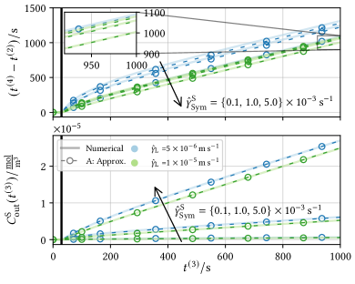
Figure 5. Top: Symport duration over the illumination duration ($t^{(1)}=$0\text{\,}\mathrm{s}$$) for different symport and leakage rates. Bottom: Corresponding change in $C^{\mathrm{S}}_{\mathrm{out}}$ during the illumination period. The vertical black line marks the minimum illumination time needed for symporter activity.

5. Conclusions

In this paper, we introduced a new ND design that can be used as an optically controlled TX in synthetic MC systems for the release of a variety of SMs using cooperating transmembrane proteins. The proposed modular design comprises an energizing module and a release module powered by the energizing module. Such a design has the potential to be useful in various future healthcare and industrial applications of MC. We proposed two analytical expressions for the concentrations of the involved molecules to describe the dynamics of the envisioned ND. The validity of the proposed solutions was successfully verified by comparison to a numerical baseline. Our model adequately captures real-world phenomena such as the presence of a pH buffer and substrate depletion in the vesicle. Our results demonstrate that the choice of appropriate system parameters, such as the ratio of pumps and co-transporters or the buffer molarity, is crucial for ensuring successful optical-to-chemical signal conversion. Consequently, the proposed analytical solutions can guide the design of future experiments and thereby accelerates the development time of the envisioned ND by offering possibilities for optimization of the system parameters to be used in practical realizations. In future work, our models will be tested and refined for further types of excitation signals, e.g., cases where the release module remains inactive. Additionally, the model will be generalized to a system containing multiple NDs, which is a crucial step towards an even more realistic system model.

References

- (1) Arman Ahmadzadeh, Vahid Jamali and Robert Schober “Molecule Harvesting Transmitter Model for Molecular Communication Systems” In IEEE Open J. Commun. Soc. 3, 2022, pp. 391–410 DOI: 10.1109/OJCOMS.2022.3155648
- (2) Hamidreza Arjmandi, Arman Ahmadzadeh, Robert Schober and Masoumeh Nasiri Kenari “Ion Channel Based Bio-Synthetic Modulator for Diffusive Molecular Communication” In IEEE Trans. Nanobioscience 15, 2016, pp. 418–432 DOI: 10.1109/TNB.2016.2557350
- (3) Christian Bamann, Ernst Bamberg, Josef Wachtveitl and Clemens Glaubitz “Proteorhodopsin” In Biochim. Biophys. Acta Bioenerg. 1837.5, 2014, pp. 614–625 DOI: https://doi.org/10.1016/j.bbabio.2013.09.010
- (4) Ajoy C. Chakrabarti and David W. Deamer “Permeability of lipid bilayers to amino acids and phosphate” In Biochim. Biophys. Acta Biomembr. 1111, 1992, pp. 171–177 DOI: 10.1016/0005-2736(92)90308-9
- (5) D.. Deamer “Proton permeation of lipid bilayers” In J. Bioenerg. Biomembr. 19, 1987, pp. 457–479 DOI: 10.1007/BF00770030
- (6) Andrei K Dioumaev et al. “Proton Transport by Proteorhodopsin Requires that the Retinal Schiff Base Counterion Asp-97 Be Anionic” In Biochemistry 42 American Chemical Society, 2003, pp. 6582–6587 DOI: 10.1021/bi034253r
- (7) George Ellison, Jon V Straumfjord and J P Hummel “Buffer Capacities of Human Blood and Plasma” In Clin. Chem. 4, 1958, pp. 452–461 DOI: 10.1093/clinchem/4.6.452
- (8) Martin Foltz et al. “Kinetics of bidirectional H+ and substrate transport by the proton-dependent amino acid symporter PAT1” In Biochem. J. 386, 2005, pp. 607–616 DOI: 10.1042/BJ20041519
- (9) Roland Goers et al. “Optimized reconstitution of membrane proteins into synthetic membranes” In Commun. Chem. 1, 2018 DOI: 10.1038/s42004-018-0037-8
- (10) Chetan T. Goudar, Jagadeesh R. Sonnad and Ronald G. Duggleby “Parameter estimation using a direct solution of the integrated Michaelis-Menten equation” In Biochim. Biophys. Acta Protein Struct. Mol. Enzymol., 1999, pp. 377–383 DOI: 10.1016/S0167-4838(98)00247-7
- (11) Laura Grebenstein et al. “Biological Optical-to-Chemical Signal Conversion Interface: A Small-Scale Modulator for Molecular Communications”, 2019 DOI: 10.1109/TNB.2018.2870910
- (12) Christian Grossmann, Hans-Georg Roos and Martin Stynes “Numerical Treatment of Partial Differential Equations” Springer, 2007, pp. 23–124 DOI: 10.1007/978-3-540-71584-9˙2
- (13) Daniel Harder et al. “Light Color‐Controlled pH‐Adjustment of Aqueous Solutions Using Engineered Proteoliposomes” In Adv. Sci., 2024 DOI: 10.1002/advs.202307524
- (14) Orlie Levy, Antonio De Vieja and Nancy Carrasco “The Na+/I– Symporter (NIS): Recent Advances” In J. Bioenerg. Biomembr. 30, 1998, pp. 195–206 DOI: 10.1023/A:1020577426732
- (15) Tatsunosuke Nakamura, Ching Hsu and Barry P. Rosen “Cation/Proton Antiport Systems in Escherichia coli” In J. Biol. Chem. 261, 1986, pp. 678–683
- (16) Tadashi Nakano, Andrew W. Eckford and Tokuko Haraguchi “Molecular Communication” Cambridge University Press, 2013 DOI: 10.1017/CBO9781139149693
- (17) Adam Noel, Dimitrios Makrakis and Abdelhakim Hafid “Channel Impulse Responses in Diffusive Molecular Communication with Spherical Transmitters” In Proc. Biennial Symp. Commun., 2016
- (18) Reinhart A.F. Reithmeier et al. “Band 3, the human red cell chloride/bicarbonate anion exchanger (AE1, SLC4A1), in a structural context” In Biochim. Biophys. Acta Biomembr. 1858, 2016 DOI: 10.1016/j.bbamem.2016.03.030
- (19) Emeline Rideau et al. “Liposomes and polymersomes: A comparative review towards cell mimicking” In Chem. Soc. Rev. 47, 2018, pp. 8572–8610 DOI: 10.1039/C8CS00162F
- (20) Renae M. Ryan, Emma L.R. Compton and Joseph A. Mindell “Functional Characterization of a Na+-dependent Aspartate Transporter from Pyrococcus horikoshii” In J. Biol. Chem. 284, 2009, pp. 17540–17548 DOI: 10.1074/jbc.M109.005926
- (21) Maximilian Schäfer et al. “Controlled signaling and transmitter replenishment for MC with functionalized nanoparticles” In Proc. 9th ACM Int. Conf. Nanosc. Comp. Commun. ACM, 2022 DOI: 10.1145/3558583.3558853
- (22) B Schobert and J K Lanyi “Halorhodopsin is a light-driven chloride pump.” In J. Biol. Chem. 257, 1982, pp. 10306–10313 DOI: 10.1016/S0021-9258(18)34020-1
- (23) Christian A. Söldner et al. “A Survey of Biological Building Blocks for Synthetic Molecular Communication Systems” In IEEE Commun. Surv. Tutor. 22, 2020, pp. 2765–2800 DOI: 10.1109/COMST.2020.3008819
- (24) Mirko Stauffer, Zöhre Ucurum, Daniel Harder and Dimitrios Fotiadis “Engineering and functional characterization of a proton-driven beta-lactam antibiotic translocation module for bionanotechnological applications” In Sci. Rep. 11, 2021, pp. 17205 DOI: 10.1038/s41598-021-96298-4
- (25) Axel Tubbe and Thomas J. Buckhout “In Vitro Analysis of the H+–Hexose Symporter on the Plasma Membrane of Sugarbeets (Beta vulgaris L.)” In Plant Physiol. 99, 1992, pp. 945–951 DOI: 10.1104/pp.99.3.945
- (26) Giovanni Zifarelli, Paolo Soliani and Michael Pusch “Buffered Diffusion around a Spherical Proton Pumping Cell: A Theoretical Analysis” In Biophys. J. 94.1, 2008, pp. 53–62 DOI: https://doi.org/10.1529/biophysj.107.111310