Primitive Heavy-ball Dynamics Achieves $O(\varepsilon^{-7/4})$ Convergence for Nonconvex Optimization

Abstract

First-order optimization methods for nonconvex functions with Lipschitz continuous gradients and Hessian have been studied intensively in both machine learning and optimization. State-of-the-art methods finding an $\varepsilon$-stationary point within $O(\varepsilon^{-{7/4}})$ or $\tilde{O}(\varepsilon^{-{7/4}})$ gradient evaluations are based on Nesterov’s accelerated gradient descent (AGD) or Polyak’s heavy-ball method. However, these algorithms employ additional mechanisms, such as restart schemes and negative curvature exploitation, which complicate the algorithms’ behavior and make it challenging to apply them to more advanced settings (e.g., stochastic optimization). To realize a simpler algorithm, we investigate the heavy-ball differential equation, a continuous-time analogy of the AGD and heavy-ball methods; we prove that the dynamics attains an $\varepsilon$-stationary point within $O(\varepsilon^{-{7/4}})$ time. We also show that a vanilla heavy-ball algorithm, obtained by discretizing the dynamics, achieves the complexity of $O(\varepsilon^{-{7/4}})$ under an additional assumption.

Keywords:

Nonconvex optimization, First-order method, Polyak’s heavy-ball method, Complexity analysis, Differential equation

MSC2020:

90C26, 90C30, 65K05, 90C06

1 Introduction

We consider general nonconvex optimization problems:

$$\min_{x\in{{\mathbb{R}}^{d}}}f(x),$$ (1)

where $f\colon{{\mathbb{R}}^{d}}\to{\mathbb{R}}$ is twice differentiable, possibly nonconvex, and lower bounded, i.e., $\inf_{x\in{{\mathbb{R}}^{d}}}f(x)>-\infty$. In machine learning, optimization problems of this form often involve a large dimension $d$, and first-order methods, which utilize only the information of the function value and gradient of $f$, are widely employed to solve these problems. First-order methods aimed at finding an $\varepsilon$-stationary point (i.e., a point $x\in{{\mathbb{R}}^{d}}$ such that $\norm{\nabla f(x)}\leq\varepsilon$) with fewer function/gradient evaluations are actively being researched in both the fields of machine learning and optimization [10, 2, 38, 19, 23, 51, 8, 33, 47, 24, 1, 13, 3, 50, 27, 28, 22, 21].

A classical result is that the gradient descent (GD) method finds an $\varepsilon$-stationary point within $O(\varepsilon^{-2})$ gradient evaluations under the Lipschitz assumption of $\nabla f$ [30]. It has also been proven that this complexity bound cannot be improved under the same assumptions [4]. From a practical perspective, the advantage of GD lies in the simplicity of the algorithm, which is expressed as a single loop without any conditional branches. Thus, the theoretical results of GD can be extended to more advanced problem settings, including finite-sum and online optimization. Many algorithms with complexity bounds, such as SGD [40, 10, 2], SVRG [38], and others [19, 23, 51, 8, 33, 47, 24], are designed by building upon the foundation of GD.

Another line of research aims to achieve better complexity bounds than GD by imposing stronger assumptions on the function $f$. Several first-order methods [1, 13, 3, 50, 27, 28, 22, 21] achieve a complexity bound of ${O\lparen\varepsilon^{-7/4}\rparen}$ or ${\tilde{O}\lparen\varepsilon^{-7/4}\rparen}$ under the Lipschitz continuity of the Hessian, in addition to the gradient. These algorithms are based not on GD but on momentum methods, specifically Nesterov’s accelerated gradient descent (AGD) [29] or Polyak’s heavy-ball (HB) method [34]. In addition, these algorithms incorporate additional mechanisms for improving complexity that are not present in GD-like methods, such as restart schemes and negative curvature exploitation. These mechanisms introduce conditional branching into the algorithm, complicating its behavior and making it difficult to extend the algorithms and their theoretical guarantees to advanced problem settings.

When considering the aforementioned two lines of research together, a natural question arises: Are additional mechanisms, such as restart schemes, essential to achieve better computational complexity than GD? More precisely, is it possible to construct a first-order method that satisfies the following two properties?

• The algorithm finds an $\varepsilon$-stationary point within ${O\lparen\varepsilon^{-7/4}\rparen}$ function/gradient evaluations under the Lipschitz assumption on the gradient and Hessian.

• The algorithm is expressed as a single loop without any conditional branches.

Considering that some first-order methods [14, 44, 46, 29] for convex optimization, including AGD, achieve optimal complexity without any conditional branches, it is natural to pursue such a method for nonconvex optimization. If such a method exists, it would be not only theoretically elegant but also practically desirable, as it would open the door to extending state-of-the-art first-order methods to more advanced settings.

Our contribution.

To explore the possibility of such a first-order method, we first analyze the HB ordinary differential equation (ODE), which serves as a common continuous-time analogy for both AGD and HB methods. We prove that, under the Lipschitz assumption on the gradient and Hessian and a specific parameter setting, a certain point computed from the solution trajectory of the HB-ODE reaches an $\varepsilon$-stationary point within ${O\lparen\varepsilon^{-7/4}\rparen}$ time. We also show that the HB algorithm, derived by discretizing the ODE, finds an $\varepsilon$-stationary point within ${O\lparen\varepsilon^{-7/4}\rparen}$ gradient evaluations under an additional assumption (Assumption 2). The resulting HB algorithm, like GD, is described by a single loop and does not include any conditional branching, making it simple.

The HB method involves a momentum parameter $\theta$, which should be appropriately set to achieve fast convergence. Various values for $\theta$ have been proposed for both convex and nonconvex optimization [34, 28, 22, 9, 20], and we propose setting $\theta=1-\Theta(K^{-1/7})$, where $K$ is the total iteration number of the algorithm. This somewhat tricky setting of the momentum parameter derives from our ODE analysis and is the first one, to the best of our knowledge.

Notation.

For $x,y\in{{\mathbb{R}}^{d}}$, let ${\left\langle{x},{y}\right\rangle}$ denote the inner product of $x$ and $y$ and $\norm{x}$ denote the Euclidean norm. For a matrix $A\in{\mathbb{R}}^{m\times n}$, let $\norm{A}$ denote the operator norm of $A$, which is equal to the largest singular value of $A$. We write the derivative of $x\colon{\mathbb{R}}\to{{\mathbb{R}}^{d}}$ as $\dot{x}(t)\coloneqq\derivative{x(t)}{t}$.

2 Related work

First-order methods with complexity bounds of ${O\lparen\varepsilon^{-7/4}\rparen}$ or ${\tilde{O}\lparen\varepsilon^{-7/4}\rparen}$.

Existing first-order methods that achieve complexity bounds of ${O\lparen\varepsilon^{-7/4}\rparen}$ or ${\tilde{O}\lparen\varepsilon^{-7/4}\rparen}$ under the Lipschitz continuity of the gradient and Hessian are summarized in Table 1. Carmon et al. [3] first developed a first-order method with ${\tilde{O}\lparen\varepsilon^{-7/4}\rparen}$ complexity; the algorithm is rather complicated, iteratively solving regularized subproblems with AGD and also exploiting negative curvature directions of $f$. Subsequently, several other algorithms with the same complexity have been proposed [1, 50, 13]. Li and Lin [21] improved the complexity to ${O\lparen\varepsilon^{-7/4}\rparen}$, and some other methods also achieved the same complexity [27, 28, 22]. An important motivation behind the research above is not only to improve complexity but also to simplify the algorithms. In fact, the more recent algorithms are simpler and more practical. The methods in [21, 27, 28, 22] achieve superior complexity bounds with restart schemes that are relatively simple compared to iteratively solving subproblems or exploiting negative curvature. The vanilla HB method analyzed in this paper has no additional mechanisms, including a restart scheme, though it requires an additional assumption for its complexity bound.

Table 1: First-order methods under the Lipschitz assumption on the graidnet and Hessian. The method in this work needs an additional assumption, Assumption 2, to achieve the complexity bound.

	Complexity	Based on	Additional mechanisms
[1, 50]	${\tilde{O}\lparen\varepsilon^{-7/4}\rparen}$	AGD	Subproblem, Negative curvature, Randomness
[3]	${\tilde{O}\lparen\varepsilon^{-7/4}\rparen}$	AGD	Subproblem, Negative curvature
[13]	${\tilde{O}\lparen\varepsilon^{-7/4}\rparen}$	AGD	Negative curvature, Randomness
[27, 21]	${O\lparen\varepsilon^{-7/4}\rparen}$	AGD	Restart
[28, 22]	${O\lparen\varepsilon^{-7/4}\rparen}$	HB	Restart
This work	${O\lparen\varepsilon^{-7/4}\rparen}$	HB	None

Heavy-ball method.

Polyak’s heavy-ball method [34] and its variants [43, 16, 39, 5] are widely applied to nonconvex optimization problems in machine learning. Despite its great practical success, studies on the theoretical performance of the HB method without restart schemes are limited. O’Neill and Wright [32] showed that the original HB is unlikely to converge to strict saddle points. Ochs et al. [31] proposed a proximal variant of HB with a complexity bound of $O(\varepsilon^{-2})$ under the Lipschitz assumption for gradients.

ODE analysis for optimization.

The advantage of studying ODEs for optimization algorithms is that it is easier to understand the behavior of continuous dynamics than the algorithm itself. Su et al. [41] considered the validity of the AGD method for convex optimization from the viewpoint of the stability of numerical schemes of ODEs. Other extensions of AGD and HB are investigated in [15, 17, 26, 48] to handle more general convex cases. Finding a Lyapunov function is a typical approach to proving an ODE’s convergence rate, especially for convex cases [49, 35, 25]. Le [18] uses a trajectory of differential inclusion to prove the convergence of a stochastic HB method for nonsmooth and nonconvex functions. This paper employs a different approach; we consider an average trajectory and evaluate gradients along that trajectory.

3 Analysis of Heavy-ball ODE

This section focuses on the following ordinary differential equation (ODE):

$$\ddot{x}(t) =-\alpha\dot{x}(t)-\nabla f(x(t)),\quad x(0)=x_{0},\quad\dot{x}(0)=0,$$ (2)

where $\alpha>0$ is a fixed parameter. This ODE can be regarded as the equation of motion for a particle moving under the influence of a conservative force $-\nabla f(x(t))$ and a frictional force $-\alpha\dot{x}(t)$. Since discretizing the ODE yields an update rule for the heavy-ball method, the ODE is useful for analyzing the heavy-ball method.

We analyze the ODE 2 under the following assumption:

Assumption 1.

For some $L_{1},L_{2}>0$,

1. $\norm{\nabla f(y)-\nabla f(x)}\leq L_{1}\norm{y-x}$ for all $x,y\in{{\mathbb{R}}^{d}}$,

2. $\norm{{\nabla^{2}}f(y)-{\nabla^{2}}f(x)}\leq L_{2}\norm{y-x}$ for all $x,y\in{{\mathbb{R}}^{d}}$.

3.1 Convergence rate for the heavy-ball ODE

To achieve fast convergence, we consider the average trajectory of the ODE solution:

$${\bar{x}}(t) \coloneqq\int_{0}^{t}w_{t}(s)x(s)\differential s$$ (3)

for $t>0$ and $\bar{x}(0)\coloneqq x(0)$, where $w_{t}\colon[0,t]\to[0,\infty[$ is a weight function such that $\int_{0}^{t}w_{t}(s)\differential s=1$. Such average solutions have also been considered in the analysis of existing first-order methods [27, 21, 28, 22] based on AGD or HB for nonconvex optimization. In this paper, we set the weight $w_{t}$ in a somewhat tricky manner as

$$w_{t}(s)\coloneqq\frac{\alpha e^{\alpha s}}{e^{\alpha t}-1}.$$ (4)

Note that $\alpha$ in the exponent is identical to the friction coefficient in the ODE 2. This choice of the weight function plays an essential role in our convergence analysis.

The main result in this section is the following theorem. It should be remarked that this theorem evaluates the norm of gradients at $\bar{x}(t)$, not at $x(t)$ itself.

Theorem 1.

Suppose that Assumption 1 holds. Let ${\Delta_{f}}\coloneqq f(x_{0})-\inf_{x\in{{\mathbb{R}}^{d}}}f(x)$.

1. For any $\alpha>0$, the ODE 2 has a unique solution $x(t)$ on $t\geq 0$.

2. Let $T>0$ and set $\alpha$ in the ODE 2 as

   $$\alpha=\lparen 3L_{2}\rparen^{\frac{2}{7}}\left\lparen\frac{\Delta_{f}}{T}\right\rparen^{\frac{1}{7}}.$$ (5)

   Then, the following holds:

   $$\min_{0\leq t\leq T}\norm{\nabla f(\bar{x}{(t)})} \leq\frac{7}{6}(3L_{2})^{\frac{1}{7}}\left\lparen\frac{\Delta_{f}}{T}\right\rparen^{\frac{4}{7}}+O\left\lparen T^{-\frac{10}{7}}\right\rparen.$$ (6)

Theorem 1 states that $\min_{0\leq t\leq T}\norm{\nabla f\left\lparen{\bar{x}(t)}\right\rparen}=O\lparen T^{-{4}/{7}}\rparen$, which means that $\norm{\nabla f\left\lparen\bar{x}(t)\right\rparen}\leq\varepsilon$ holds for some $t={O\lparen\varepsilon^{-7/4}\rparen}$. This order is consistent with the state-of-the-art complexity bound, ${O\lparen\varepsilon^{-7/4}\rparen}$, for the first-order methods discussed in Section 2. Theorem 1 implies the possibility of developing a heavy-ball algorithm with a complexity bound of ${O\lparen\varepsilon^{-7/4}\rparen}$ without any additional mechanisms by discretizing the ODE 2.

Let us provide some additional remarks on Theorem 1. The Lipschitz constant $L_{1}$ for $\nabla f$ does not appear in the right-hand side of 6 because we use 1(a) only for the proof of 1(a). Note that the trajectories $x(t)$ and $\bar{x}(t)$ depend on $T$ since the parameter setting for $\alpha$ depends on $T$ in 1(b). Differential equations where the solution trajectory depends on the termination time are sometimes used in analysis for optimization [42, 15].

3.2 Proof sketch

The complete proof of Theorem 1 can be found in Appendix A, and this section provides a sketch of the proof. Below is a key lemma, whose proof can be found in Section A.1.

Lemma 1.

Let $t>0$ and $z\colon{{\left[{0},{t}\right]}}\rightarrow{{\mathbb{R}}^{d}}$. Suppose 1(b) holds and that a function $w\colon{{\left[{0},{t}\right]}}\rightarrow[0,\infty[$ satisfies $\int_{0}^{t}w(s)\differential s=1$. Let $\bar{z}\coloneqq\int_{0}^{t}w(s)z(s)\differential s$. Then, the following holds:

$$\norm{\nabla f(\bar{z})-\int_{0}^{t}w(s)\nabla f(z(s))\differential s}\leq\frac{L_{2}}{2}\int_{0}^{t}{{\norm{\dot{z}(s)}^{2}}}\left\lparen{\int_{0}^{s}\differential\sigma\int_{s}^{t}\differential\tau\ w(\sigma)w(\tau)(\tau-\sigma)}\right\rparen\differential s.$$ (7)

This lemma bounds the error when the gradient $\nabla f(\bar{z})$ at the average solution $\bar{z}$ is approximated by the average of the gradients $\int_{0}^{t}w(s)\nabla f(z(s))\differential s$. Applying this lemma with $(z,w)=(x,w_{t})$, where $x$ is the solution of the ODE 2 and $w_{t}$ is defined by 4, gives the following bound:

$$\norm{\nabla f(\bar{x}(t))-\int_{0}^{t}w_{t}(s)\nabla f(x(s))\differential s}\leq\frac{L_{2}}{2}\int_{0}^{t}{{\norm{\dot{x}(s)}^{2}}}\left\lparen{\int_{0}^{s}\differential\sigma\int_{s}^{t}\differential\tau\ w_{t}(\sigma)w_{t}(\tau)(\tau-\sigma)}\right\rparen\differential s.$$ (8)

Thanks to the definition 4 of the weight $w_{t}$, the average of the gradients simplifies to

$$\int_{0}^{t}w_{t}(s)\nabla f(x(s))\differential s=-w_{t}(t)\dot{x}(t)=-\frac{\alpha}{1-e^{-\alpha t}}\dot{x}(t).$$ (9)

Substituting this equation into the left-hand side of 8 and doing some calculations, we can obtain the following upper bound on $\norm{\nabla f({\bar{x}(t)})}$.

Lemma 2.

The following holds for all $t>0$:

$$\norm{\nabla f({\bar{x}(t)})}\leq\frac{\alpha}{1-e^{-\alpha t}}\norm{\dot{x}(t)}+\frac{L_{2}}{2}\frac{1}{\left\lparen 1-e^{-\alpha t}\right\rparen^{2}}\int_{0}^{t}{\norm{\dot{x}(s)}^{2}}e^{-\alpha(t-s)}\left\lparen t-s\right\rparen\differential s.$$ (10)

The proof can be found in Section A.2. Roughly speaking, this lemma implies that $\norm{\nabla f(\bar{x}(t))}$ is small if $\norm{\dot{x}(s)}$ is small for $s\in[0,t]$. We can also show that

$$\int_{0}^{t}{\norm{\dot{x}(s)}^{2}}\differential s\leq\frac{{\Delta_{f}}}{\alpha}$$ (11)

from the relationship between mechanical energy and the work done by friction in the ODE 2. Combining 11 together with Lemma 2 yields the following upper bound for all $T>0$:

$$\left\lparen T-\frac{3}{2\alpha}\right\rparen\min_{0\leq t\leq T}\norm{\nabla f({\bar{x}(t)})} \leq\sqrt{\alpha T{\Delta_{f}}}+\frac{L_{2}{\Delta_{f}}}{2\alpha^{3}}.$$ (12)

The parameter $\alpha$ in 5 is chosen to minimize the right-hand side of the above inequality. Substituting that $\alpha$ into the inequality gives the desired result 6.

4 Analysis of (Discrete-time) Heavy-ball algorithm

This section discusses the complexity of the heavy-ball algorithm, obtained by discretizing the continuous system 2. We show that the algorithm finds an $\varepsilon$-stationary point within ${O\lparen\varepsilon^{-7/4}\rparen}$ gradient evaluations under a certain assumption derived from the discretization.

4.1 Algorithm and parameter setting

Let us consider the discretization of 2 with discretization width ${h}$. For sufficiently small ${h}>0$, $\dot{x}(t)$ and $\ddot{x}(t)$ can be approximated as

$$\dot{x}(t) \approx\frac{x(t)-x(t-{h})}{{h}}\quad\text{and}\quad\ddot{x}(t)\approx\frac{1}{{h}}\left\lparen\frac{x(t+{h})-x(t)}{{h}}-\frac{x(t)-x(t-{h})}{{h}}\right\rparen,$$ (13)

respectivly. Then, 2 is approximated as

$$\frac{1}{{h}}\left\lparen\frac{x(t+{h})-x(t)}{{h}}-\frac{x(t)-x(t-{h})}{{h}}\right\rparen=-\alpha\frac{x(t)-x(t-{h})}{{h}}-\nabla f(x(k{h})),$$ (14)

and rearranging the terms yields the update rule for Polyak’s heavy-ball method [34]:

$$x_{k+1}=x_{k}+\theta\left\lparen x_{k}-x_{k-1}\right\rparen-\eta\nabla f(x_{k}),$$ (15)

where we set

$$x_{k}\approx x(t),\quad k{h}=t,\quad\theta=1-\alpha{{h}},\quad\eta={h}^{2}.$$ (16)

Here, $\eta>0$ and $\theta\in{\left[{0},{1}\right]}$ are called the step-size and momentum parameters, respectively. Let $x_{-1}=x_{0}$ for simplicity. Another interpretation of the derivation of the update rule 15 in the opposite direction is that taking the limit of ${h}\to+0$ (also ${\eta}\to+0$) on 15 with the relationship 16 recovers the ODE 2.

As in Section 3, we will show that the gradient at an average solution is small; as a counterpart to 3 and 4, we define the average solution by

$$\bar{x}_{k}\coloneqq\sum_{i=0}^{k-1}p_{k,i}x_{i},\quad\text{where}\quad p_{k,i}\coloneqq\frac{1-\theta}{1-\theta^{k}}\theta^{k-1-i}.$$ (17)

Note that $\sum_{i=0}^{k-1}p_{k,i}=1$. The weight $p_{k,i}$ is a discrete analogy to $w_{t}(s)$ defined by 4. Taking the limit $h\to+0$ with the relationship 16 and $s=i{h}$, we have

$$\frac{p_{k,i}}{{h}}=\frac{1}{h}\frac{\alpha h}{1-(1-\alpha h)^{t/h}}(1-\alpha h)^{(t-s)/h-1}\to\alpha\frac{e^{-\alpha(t-s)}}{1-e^{-\alpha t}}=w_{t}(s),$$ (18)

and thus $\bar{x}_{k}\to\bar{x}(t)$ as $h\to+0$.

The heavy-ball algorithm analyzed in this section is described in Algorithm 1. We note that the average solution $\bar{x}_{k}$ is efficiently computable with a simple recursion (see Section C.2).

Algorithm 1 Heavy-Ball method for nonconvex functions

1:$x_{0}\in{{\mathbb{R}}^{d}}$, $\eta>0$, $\theta\in[0,1]$, and $K>0$

2:$x_{-1}=x_{0}$

3:for $k=1,\dots,K$ do

4:     $\bar{x}_{k}=\sum_{i=0}^{k-1}\frac{1-\theta}{1-\theta^{k}}\theta^{k-1-i}x_{i}$

5:     $x_{k}=x_{k-1}+\theta\left\lparen x_{k-1}-x_{k-2}\right\rparen-\eta\nabla f(x_{k-1})$

6:return $\operatorname*{argmin}_{x\in\{\bar{x}_{1},\dots,\bar{x}_{K}\}}{\norm{\nabla f\left\lparen{x}\right\rparen}}$

To achieve theoretically fast convergence, it is crucial to determine appropriate values for the parameters $\eta$ and $\theta$. We propose setting these parameters as

$$\eta=\frac{2}{L_{1}}\quad\text{and}\quad\theta=1-\frac{\beta}{K^{1/7}},$$ (19)

where $L_{1}$ is the Lipschitz constant for $\nabla f$, $K$ is the total iteration number, and $\beta>0$ is a constant. We only consider the case where $K>\beta^{7}$ to satisfy $\theta>0$. Note that $K$ should be determined before running the algorithm in order to set the momentum parameter $\theta$.

Existing heavy-ball methods [22, 28] that achieve ${O\lparen\varepsilon^{-7/4}\rparen}$ complexity with restart schemes set the momentum parameter to $\theta=1-1/K$ [22] or $\theta=1$ [28]. Our somewhat tricky choice of $\theta=1-\Theta(K^{-1/7})$ is inspired by the ODE analysis in Section 3; the intuition derives from the fact that $\alpha=\Theta(T^{-1/7})$ in 5 is optimal for the continuous system and the relationship given in 16.

4.2 Complexity analysis

We analyze Algorithm 1 in a manner parallel to Section 3.2. The complete proof for this section can be found in Appendix B, and this section provides a sketch of the proof.

Using the discrete version of Lemma 1 (see Lemma 6 in Section B.1), we can obtain the following bound, a discrete-time analogy to 8:

$$\norm{\nabla f(\bar{x}_{k})-\sum_{i=0}^{k-1}p_{k,i}\nabla f(x_{i})}\leq\frac{L_{2}}{2}\sum_{i=1}^{k-1}{\norm{{x_{i}-x_{i-1}}}^{2}}\sum_{0\leq\sigma<i\leq\tau<k}(\tau-\sigma)p_{k,\sigma}p_{k,\tau}.$$ (20)

Thanks to definition 17 of $p_{k,i}$, the average of the gradients simplifies to

$$\sum_{i=0}^{k-1}p_{k,i}\nabla f(x_{i})=-\frac{p_{k,k-1}}{\eta}(x_{k}-x_{k-1})=-\frac{1}{\eta}\frac{1-\theta}{1-\theta^{k}}(x_{k}-x_{k-1}).$$ (21)

Substituting 21 into the left-hand side of 20 yields the following upper bound on $\norm{\nabla f\left\lparen{\bar{x}_{k}}\right\rparen}$, an analogy of Lemma 2. Its proof can be found in Section B.2.

Lemma 3.

The following holds for all $k\geq 1$:

$$\norm{\nabla f\left\lparen{\bar{x}_{k}}\right\rparen}\leq\frac{1}{\eta}\frac{1-\theta}{1-\theta^{k}}\norm{x_{k}-x_{k-1}}+\frac{L_{2}}{2\left\lparen 1-\theta^{k}\right\rparen^{2}}\sum_{i=1}^{k-1}\theta^{k-i}\left\lparen k-i\right\rparen{\norm{x_{i}-x_{i-1}}^{2}}.$$ (22)

Next, similar to the analysis of the continuous system, we aim to derive an upper bound for $\sum_{i}{\norm{x_{i}-x_{i-1}}^{2}}$. While the upper bound 11 was relatively straightforward to obtain, discretization errors make the proof difficult in the discrete-time case. In fact, as shown in the following lemma, upper-bounding $\sum_{i}{\norm{x_{i}-x_{i-1}}^{2}}$ introduces an additional term of $\sum_{i}\norm{x_{i}-x_{i-1}}^{3}$.

Lemma 4.

If $\eta\leq\frac{2}{L_{1}}$, the following holds for all $k\geq 1$:

$$(1-\theta)\left\lparen\frac{1}{\eta}-\frac{L_{1}}{2(1+\theta)}\right\rparen\sum_{i=1}^{k}{\norm{x_{i}-x_{i-1}}^{2}}\leq\Delta_{f}+\frac{L_{2}\theta}{6\left\lparen\theta+1\right\rparen}\sum_{i=1}^{k}\norm{x_{i}-x_{i-1}}^{3}.$$ (23)

The proof can be found in Section B.3. Let us verify that the above inequality corresponds to 11 despite the additional term. It follows from the relationship 16 that

$$\norm{\frac{x_{k}-x_{k-1}}{h}}\approx\norm{\dot{x}(kh)}=\norm{\dot{x}(t)},$$ (24)

as $h\to+0$. With 16, we have

$$(1-\theta)\left\lparen\frac{1}{\eta}-\frac{L_{1}}{2(1+\theta)}\right\rparen\sum_{i=1}^{k}{\norm{x_{i}-x_{i-1}}^{2}} =\alpha\left\lparen 1-\frac{L_{1}h^{2}}{2\left\lparen 2-\alpha h\right\rparen}\right\rparen\sum_{i=1}^{k}{\norm{\frac{x_{i}-x_{i-1}}{h}}^{2}}h$$ (25)

$$\approx\alpha\int_{0}^{t}{\norm{\dot{x}(s)}^{2}}\differential s,$$ (26)

as $h\to+0$. We can also check that the right-hand side of Lemma 4 goes to $\Delta_{f}$ as $h\to+0$, which is consistent with 11. See Section C.1 for a more detailed discussion.

We make the assumption that the term of $\sum_{i}\norm{x_{i}-x_{i-1}}^{3}$ is bounded, which is negligibly small if $\eta$ is small, as discussed above.

Assumption 2.

There exists a constant $C>0$ such that

$$\sum_{i=1}^{K}{\norm{x_{i}-x_{i-1}}}^{3}\leq{{C}}.$$ (27)

This assumption holds, for example, when $\norm{x_{k}-x_{k-1}}$ converges to zero at a rate of $\norm{x_{k}-x_{k-1}}=o(k^{-1/3-\delta})$, where $\delta>0$. With the help of Assumption 2, we obtain the following complexity bound for Algorithm 1. Its complete proof can be found in Section B.4.

Theorem 2.

Suppose that Assumption 1 holds. Assume that Algorithm 1 with the parameters set as in 19 satisfies Assumption 2. Then, the output $x_{\star}\in{{\mathbb{R}}^{d}}$ of Algorithm 1 satisfies

$$\norm{\nabla f\left\lparen{x_{\star}}\right\rparen} \leq\left\lparen\sqrt{L_{1}\beta}\left\lparen{\Delta_{f}}+{{\frac{L_{2}C}{12}}}\right\rparen^{\frac{1}{2}}+\frac{2L_{2}}{L_{1}\beta^{3}}\left\lparen{\Delta_{f}}+{{\frac{L_{2}C}{12}}}\right\rparen\right\rparen{K^{-\frac{4}{7}}}+O\left\lparen K^{-\frac{5}{7}}\right\rparen.$$ (28)

Theorem 2 states that $\norm{\nabla f\left\lparen{x_{\star}}\right\rparen}=O\lparen K^{-{4}/{7}}\rparen$ holds. Hence, $K={O\lparen\varepsilon^{-7/4}\rparen}$ iterations suffice to find an $\varepsilon$-stationary point, which is the same as the existing complexity bound. The constant $\beta>0$ that determines $\theta=1-\beta K^{-1/7}$ can also be arbitrarily changed, but it is difficult to determine the optimal $\beta$ from 28 without the knowledge of $L_{1}$, $L_{2}$, $\Delta_{f}$, and $C$.

5 Numerical experiments

This section compares the performance of Algorithm 1 with several existing algorithms. We implemented the code in Python by modifying the code for [28] and executed them on a computer with an 11th Gen Intel Core i5 CPU processor and 16GiB RAM.

5.1 Compared methods

We compare the following six methods:

• Proposed: Algorithm 1.

• GD: The gradient descent method with Armijo-type backtracking.

• JNJ2018 [13]: Accelerated gradient descent (AGD) method with negative curvature exploitation.

• LL2022 [21] and MT2022 [27]: AGD with restart scheme.

• MT2023 [28]: Heavy-ball method with restart scheme.

See Section C.3 for their parameter settings.

5.2 Problem instances

We tested the algorithms with five types of instances. The first three instances are benchmark functions from [12]: Dixon–Price function [7], Powell function [36], and Qing function [37]. The parameter settings for these functions are stated in Section C.3. The other two instances are standard instances in machine learning.

One is training a neural network for classification with the MNIST dataset [6]:

$$\min_{w\in{\mathbb{R}}^{d}}\ \frac{1}{N}\sum_{i=1}^{N}\ell_{\mathrm{CE}}(y_{i},\phi_{1}(x_{i};w)),$$ (29)

Here, the vectors $x_{1},\dots,x_{N}\in{\mathbb{R}}^{M}$ and $y_{1},\dots,y_{N}\in\{0,1\}^{K}$ are given data, $\ell_{\mathrm{CE}}$ is the cross-entropy loss, and $\phi_{1}(\cdot;w)\colon{\mathbb{R}}^{M}\to{\mathbb{R}}^{K}$ is a neural network parameterized by $w\in{\mathbb{R}}^{d}$. We used a three-layer fully connected network with bias parameters. The number of the nodes in each layer is $M=784$, $32$, $16$, and $K=10$, respectively. The hidden layers have the logistic sigmoid activation, and the output layer has the softmax activation. The dimension of the parameter space is $d=(784\times 32+32\times 16+16\times 10)+(32+16+10)=25818$. The data size is $N=10000$.

The other is low-rank matrix completion with the MovieLens-100K dataset [11]:

$$\min_{\begin{subarray}{c}U\in{\mathbb{R}}^{p\times r}\\ V\in{\mathbb{R}}^{q\times r}\end{subarray}}\ \frac{1}{2N}\sum_{(i,j,s)\in\Omega}\left\lparen(UV^{\top})_{ij}-s\right\rparen^{2}+\frac{1}{2N}\norm*{U^{\top}U-V^{\top}V}_{\mathrm{F}}^{2}.$$ (30)

The set $\Omega$ consists of $N=100000$ observed entries of a $p\times q$ data matrix, and $(i,j,s)\in\Omega$ means that the $(i,j)$-th entry is $s$. The second term with the Frobenius norm $\norm{\cdot}_{\mathrm{F}}$ was introduced in [45]. The size of the data matrix is $p=943$ times $q=1682$, and we set the rank as $r\in\{100,200\}$. Consequently, the number of variables is $pr+qr\in\{262500,525000\}$.

5.3 Results

Figure 1 presents the results. In each figure, the horizontal axis represents the execution time and the vertical axis represents the objective function value or the norm of gradients.

The Dixon–Price function was most efficiently minimized by LL2022, followed by Proposed and JNJ2018. However, Proposed was the most efficient at finding points with small gradient norm. For the Powell function, MT2023 was the most efficient, and Proposed and MT2022 were the next fastest. For the Qing function, Proposed, MT2022 and MT2023 were the most efficient with similar efficiency. For the Classification task, MT2023 was the fastest followed by Proposed, LL2022. For Movielens task, when $r=100$, MT2023 and LL2022were the fastest, followed by MT2022 and Proposed. When $r=200$, Proposed was the most efficient.

Although Proposed is a simple heavy-ball method, it was as efficient as the other methods in many cases. It is attributed to the theoretical efficiency shown in Section 4 of the primitive heavy-ball method. However, the practical drawback of this method is that it has two parameters, $L_{1}$ and $\theta$, to be tuned. As we mentioned in Section 4, finding the optimal parameter $\theta$ is difficult but essentially important to reduce the complexity.

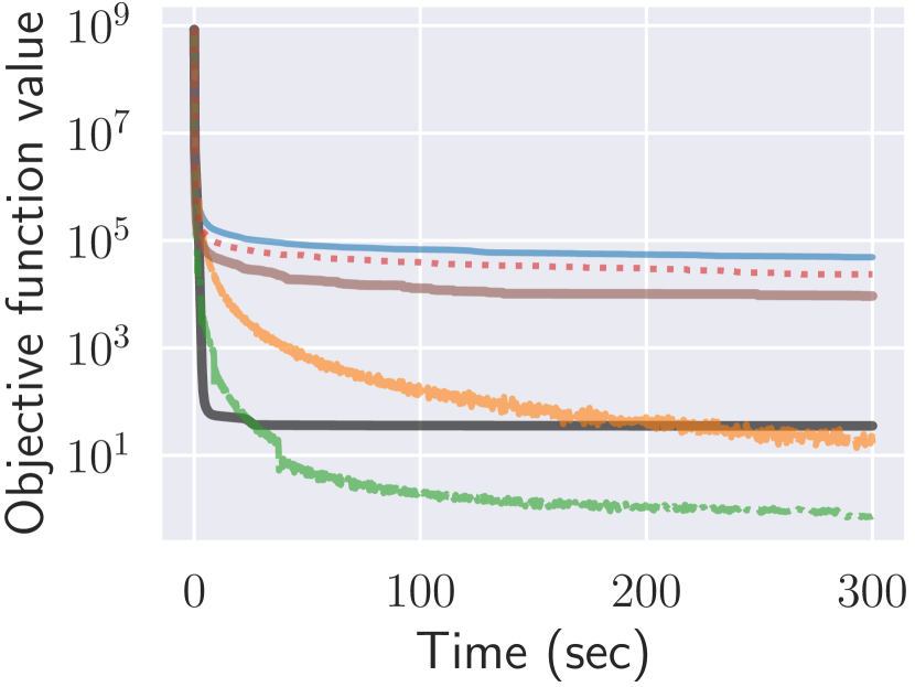
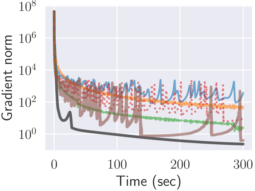
(a) Dixon–Price

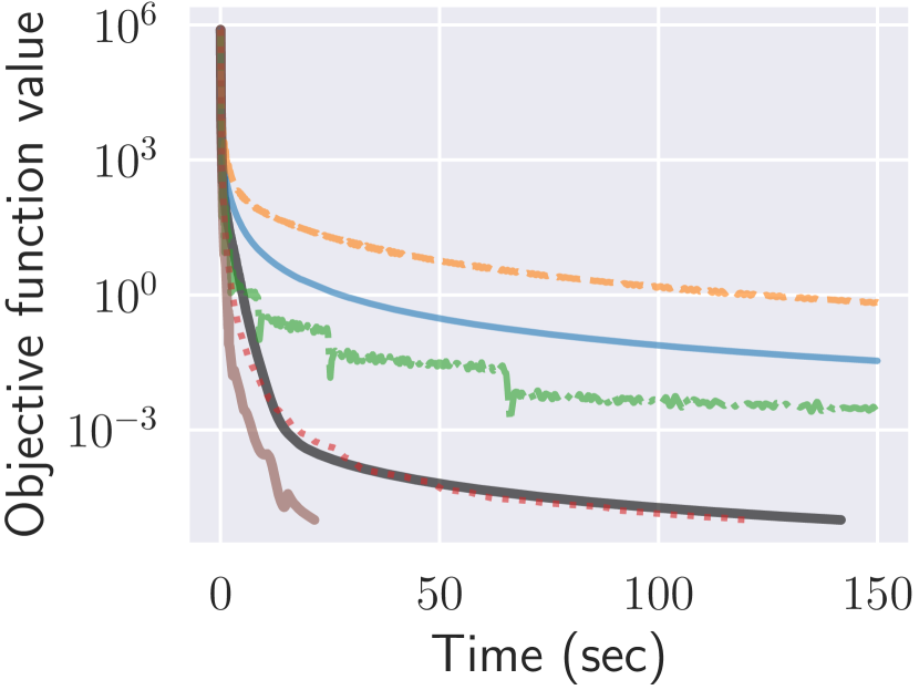
(b) Powell

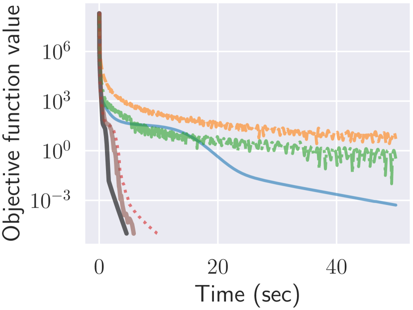
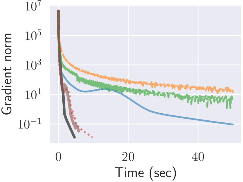
(c) Qing

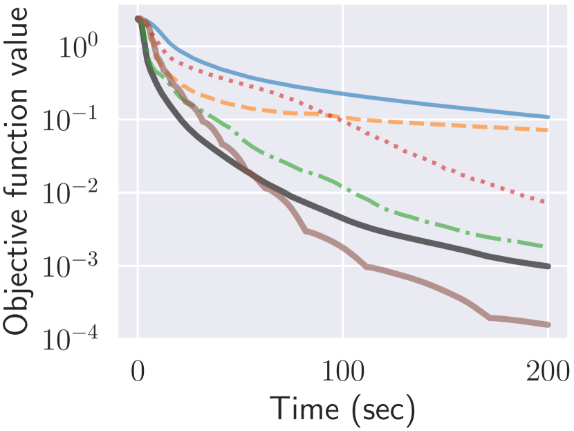
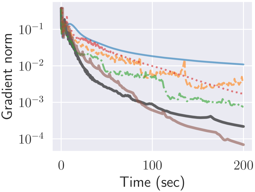
(d) Classification

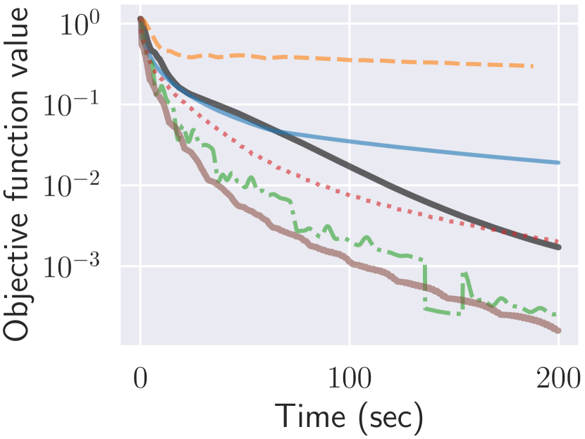
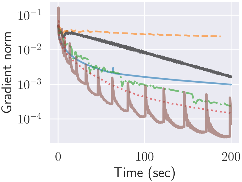
(e) Matrix completion ($r=100$)

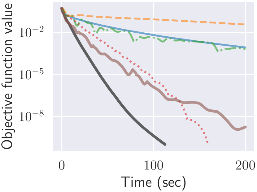
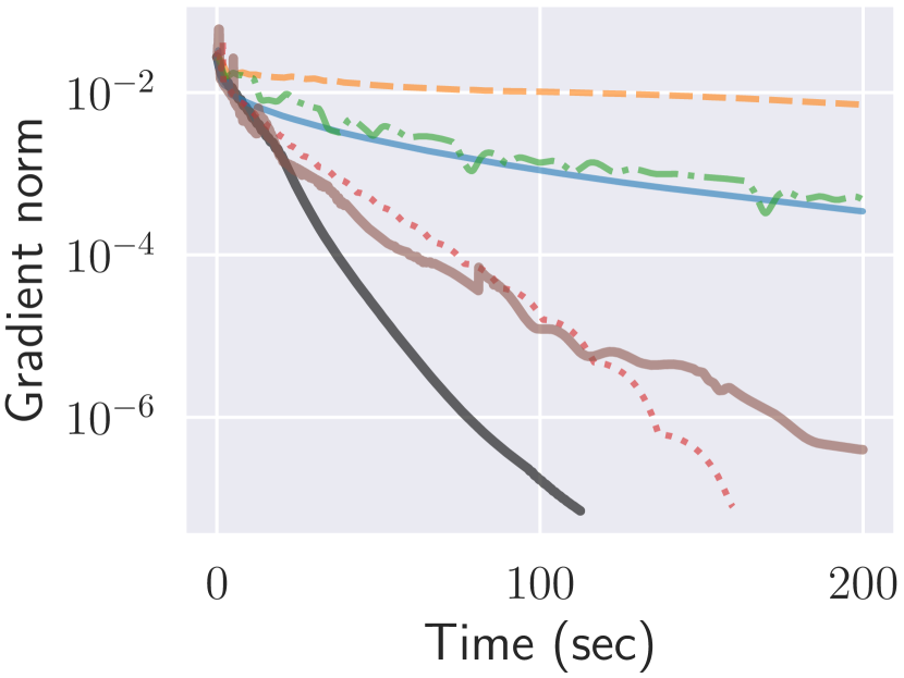
(f) Matrix completion ($r=200$)

Figure 1: Numerical results.

6 Limitations and future work

In this paper, we have discussed the heavy-ball ODE 2 and the efficiency of the primitive heavy-ball method (Algorithm 1). Theorem 1 requires only Assumption 1, while Theorem 2, due to the discretization, needs an additional assumption, Assumption 2. Improving the discretization scheme to remove or weaken this assumption and to make it easier to determine the input parameter for Algorithm 1 is the future work. Additionally, as mentioned in the introduction, applying this primitive heavy-ball algorithm and its complexity analysis to more advanced settings is also part of our future work.

Appendix A Omitted proofs for Section 3

A.1 Proof of Lemma 1

Proof.

More strongly, we show the following inequalities and equality:

$$\norm{\nabla f(\bar{z})-\int_{0}^{t}w(s)\nabla f(z(s))\differential s}$$ (31)

$$\phantom{hogehoge}\leq\frac{L_{2}}{2}\int_{0}^{t}w(s){\norm{z(s)-\bar{z}}^{2}}\differential s$$ (32)

$$\phantom{hogehoge}=\frac{L_{2}}{2}\iint_{0\leq\sigma\leq\tau\leq t}w(\sigma)w(\tau){\norm{z(\tau)-z(\sigma)}^{2}}\differential\sigma\differential\tau$$ (33)

$$\phantom{hogehoge}\leq\frac{L_{2}}{2}\int_{0}^{t}{\norm{\dot{z}(s)}^{2}}\left\lparen{\int_{0}^{s}\differential\sigma\int_{s}^{t}\differential\tau\ w(\sigma)w(\tau)(\tau-\sigma)}\right\rparen\differential s.$$ (34)

For $s\in{\left[{0},{t}\right]}$, we have

$$\nabla f(z(s))-\nabla f(\bar{z}) =\int_{0}^{1}{\nabla^{2}}f((1-\sigma)\bar{z}+\sigma z(s))(z(s)-\bar{z})\differential\sigma$$ (35)

$$={\nabla^{2}}f(\bar{z})(z(s)-\bar{z})+\int_{0}^{1}\left\lparen{\nabla^{2}}f((1-\sigma)\bar{z}+\sigma z(s))-{\nabla^{2}}f(\bar{z})\right\rparen(z(s)-\bar{z})\differential\sigma.$$ (36)

By multiplying 36 by $w(s)$ and integrating it on $s\in{\left[{0},{t}\right]}$, we have

$$\int_{0}^{t}w(s)\left\lparen\nabla f(z(s))-\nabla f(\bar{z})\right\rparen\differential s$$ (37)

$$\hskip 30.0pt=\int_{0}^{t}w(s)\left\lparen{\nabla^{2}}f(\bar{z})(z(s)-\bar{z})\right\rparen\differential s$$ (38)

$$\hskip 60.0pt+\int_{0}^{t}w(s){\int_{0}^{1}\left\lparen{\nabla^{2}}f((1-\sigma)\bar{z}+\sigma z(s))-{\nabla^{2}}f(\bar{z})\right\rparen(z(s)-\bar{z})\differential\sigma}\differential s.$$ (39)

The left-hand side of 39 is

$$\int_{0}^{t}w(s)\left\lparen\nabla f(z(s))-\nabla f(\bar{z})\right\rparen\differential s =\int_{0}^{t}w(s)\nabla f(z(s))\differential s-\nabla f(\bar{z})$$ (40)

since $\int_{0}^{t}w(s)\differential s=1$. The first term of the right-hand side of 39 is

$$\int_{0}^{t}w(s)\left\lparen{\nabla^{2}}f(\bar{z})(z(s)-\bar{z})\right\rparen\differential s ={\nabla^{2}}f(\bar{z})\int_{0}^{t}w(s)(z(s)-\bar{z})\differential s$$ (41)

$$={\nabla^{2}}f(\bar{z})\left\lparen\int_{0}^{t}w(s)z(s)\differential s-\left\lparen\int_{0}^{t}w(s)\differential s\right\rparen\bar{z}\right\rparen$$ (42)

$$={\nabla^{2}}f(\bar{z})\left\lparen\bar{z}-\bar{z}\right\rparen$$ (43)

$$=0.$$ (44)

Furthermore, the norm of the second term of the right-hand side of 39 is evaluated as follows:

$$\phantom{\leq\ }\norm{\int_{0}^{t}w(s){\int_{0}^{1}\left\lparen{\nabla^{2}}f((1-\sigma)\bar{z}+\sigma z(s))-{\nabla^{2}}f(\bar{z})\right\rparen(z(s)-\bar{z})\differential\sigma}\differential s}$$ (45)

$$\leq\int_{0}^{t}w(s){\int_{0}^{1}\norm{{\nabla^{2}}f((1-\sigma)\bar{z}+\sigma z(s))-{\nabla^{2}}f(\bar{z})}\norm{z(s)-\bar{z}}\differential\sigma}\differential s$$ (46)

$$\leq\int_{0}^{t}w(s){\int_{0}^{1}L_{2}\norm{((1-\sigma)\bar{z}+\sigma z(s))-\bar{z}}\norm{z(s)-\bar{z}}\differential\sigma}\differential s {\left\lparen\text{by }{\text{\lx@cref{creftype~refnum}{assumption:L2}}}\right\rparen}$$ (47)

$$=\int_{0}^{t}w(s)\int_{0}^{1}\sigma L_{2}{\norm{z(s)-\bar{z}}^{2}}\differential\sigma\differential s$$ (48)

$$=\frac{L_{2}}{2}\int_{0}^{t}w(s){\norm{z(s)-\bar{z}}^{2}}\differential s.$$ (49)

By taking norm of both sides of 39 and applying 40, 44 and 49, we have

$$\norm{\int_{0}^{t}w(s)\nabla f(z(s))\differential s-\nabla f(\bar{z})}\leq\frac{L_{2}}{2}\int_{0}^{t}w(s){\norm{z(s)-\bar{z}}^{2}}\differential s,$$ (50)

which is equivalent to 32.

Next we show the equality 33. Since

$${\norm{\int_{0}^{t}w(\sigma)z(\sigma)\differential\sigma}^{2}} ={\left\langle{\int_{0}^{t}w(\sigma)z(\sigma)\differential\sigma},{\int_{0}^{t}w(\tau)z(\tau)\differential\tau}\right\rangle}$$ (51)

$$=\iint_{{{\left[{0},{t}\right]}}^{2}}w(\sigma)w(\tau){\left\langle{z(\sigma)},{z(\tau)}\right\rangle}\differential\sigma\differential\tau,$$ (52)

we have

$$\iint_{0\leq\sigma\leq\tau\leq t}w(\sigma)w(\tau){\norm{z(\tau)-z(\sigma)}^{2}}\differential\sigma\differential\tau$$ (53)

$$=\frac{1}{2}\iint_{{{\left[{0},{t}\right]}}^{2}}w(\sigma)w(\tau){\norm{z(\tau)-z(\sigma)}^{2}}\differential\sigma\differential\tau$$ (54)

$$=\int_{0}^{t}w(\sigma){\norm{z(\sigma)}^{2}}\differential\sigma-\iint_{{{\left[{0},{t}\right]}}^{2}}w(\sigma)w(\tau){\left\langle{z(\sigma)},{z(\tau)}\right\rangle}\differential\sigma\differential\tau$$ (55)

$$=\int_{0}^{t}w(\sigma){\norm{z(\sigma)}^{2}}\differential\sigma-{\norm{\int_{0}^{t}w(\sigma)z(\sigma)\differential\sigma}^{2}}\quad{\left\lparen\text{by }{\lx@cref{creftype~refnum}{lemma-continuous-sublem1}}\right\rparen}$$ (56)

$$=\int_{0}^{t}w(\sigma){\norm{z(\sigma)}^{2}}\differential\sigma-{\norm{\bar{z}}^{2}}$$ (57)

$$=\int_{0}^{t}w(\sigma){\norm{z(\sigma)}^{2}}\differential\sigma-2{\norm{\bar{z}}^{2}}+{\norm{\bar{z}}^{2}}$$ (58)

$$=\int_{0}^{t}w(\sigma){\norm{z(\sigma)}^{2}}\differential\sigma-2{\left\langle{\int_{0}^{t}w(\sigma)z(\sigma)\differential\sigma},{\bar{z}}\right\rangle}+{\norm{\bar{z}}^{2}}\int_{0}^{t}w(\sigma)\differential\sigma$$ (59)

$$\phantom{daaaaaaaaaaaaaaaaaaaa}\left\lparen\text{since }{\bar{z}\coloneqq\int_{0}^{t}w(\sigma)z(\sigma)\differential\sigma\text{ and }\int_{0}^{t}w(\sigma)\differential\sigma=1}\right\rparen$$ (60)

$$=\int_{0}^{t}w(\sigma){\norm{z(\sigma)-\bar{z}}^{2}}\differential\sigma,$$ (61)

which is equivalent to 33.

Next we prove inequality 34. For $0\leq\sigma\leq\tau\leq t$, we have

$${\norm{z(\tau)-z(\sigma)}^{2}} ={\norm{\int_{\sigma}^{\tau}\dot{z}(s)\differential s}^{2}}$$ (62)

$$\leq\left\lparen{\int_{\sigma}^{\tau}\norm{\dot{z}(s)}\differential s}\right\rparen^{2} {\left\lparen\text{by }{\text{the triangle inequality}}\right\rparen}$$ (63)

$$\leq\left\lparen{\int_{\sigma}^{\tau}{\norm{\dot{z}(s)}^{2}}\differential s}\right\rparen\left\lparen\int_{\sigma}^{\tau}\differential s\right\rparen {\left\lparen\text{by }{\text{Cauchy--Schwarz inequality}}\right\rparen}$$ (64)

$$=(\tau-\sigma){\int_{\sigma}^{\tau}{\norm{\dot{z}(s)}^{2}}\differential s}.$$ (65)

Using this, we also have

$$\int_{0\leq\sigma\leq\tau\leq t}w(\sigma)w(\tau){\norm{z(\tau)-z(\sigma)}^{2}}\differential\sigma\differential\tau \leq\int_{0\leq\sigma\leq\tau\leq t}w(\sigma)w(\tau)(\tau-\sigma)\int_{\sigma}^{\tau}{\norm{\dot{z}(s)}^{2}}\differential s\differential\sigma\differential\tau$$ (66)

$$=\int_{0\leq\sigma\leq s\leq\tau\leq t}w(\sigma)w(\tau)(\tau-\sigma){{\norm{\dot{z}(s)}^{2}}\differential s}\differential\sigma\differential\tau$$ (67)

$$=\int_{0}^{t}{\norm{\dot{z}(s)}^{2}}\left\lparen{\int_{0}^{s}\differential\sigma\int_{s}^{t}\differential\tau\ w(\sigma)w(\tau)(\tau-\sigma)}\right\rparen\differential s.$$ (68)

This implies 34. ∎

A.2 Proof of Lemma 2

Proof.

Applying Lemma 1 with $(z,w)=(x,w_{t})$, where $x$ is the solution of the ODE 2 and $w_{t}$ is defined by 4, gives the following bound:

$$\norm{\nabla f(\bar{x}(t))-\int_{0}^{t}w_{t}(s)\nabla f(x(s))\differential s}\leq\frac{L_{2}}{2}\int_{0}^{t}{{\norm{\dot{x}(s)}^{2}}}\left\lparen{\int_{0}^{s}\differential\sigma\int_{s}^{t}\differential\tau\ w_{t}(\sigma)w_{t}(\tau)(\tau-\sigma)}\right\rparen\differential s.$$ (69)

Using the triangle inequality gives

$$\norm{\nabla f(\bar{x}(t))}\leq\norm{\int_{0}^{t}w_{t}(s)\nabla f(x(s))\differential s}+\frac{L_{2}}{2}\int_{0}^{t}{{\norm{\dot{x}(s)}^{2}}}\left\lparen\int_{0}^{s}\differential\sigma\int_{s}^{t}\differential\tau\ w_{t}(\sigma)w_{t}(\tau)(\tau-\sigma)\right\rparen\differential s.$$ (70)

Now, we will evaluate each term on the right-hand side. The first term is evaluated as follows:

$$\int_{0}^{t}w_{t}(s)\nabla f(x(s))\differential s =-\int_{0}^{t}w_{t}(s)\left\lparen\ddot{x}(s)+\alpha\dot{x}(s)\right\rparen\differential s {\left\lparen\text{by }{\lx@cref{creftype~refnum}{equation:ode}}\right\rparen}$$ (71)

$$=-\int_{0}^{t}\left\lparen w_{t}(s)\ddot{x}(s)+\dot{w}_{t}(s)\dot{x}(s)\right\rparen\differential s {\left\lparen\text{by }{\lx@cref{creftype~refnum}{eq:def_w}}\right\rparen}$$ (72)

$$=-\left[w_{t}(s)\dot{x}(s)\right]_{s=0}^{t}$$ (73)

$$=-w_{t}(t)\dot{x}(t)$$ (74)

$$=-\frac{\alpha}{1-e^{-\alpha t}}\dot{x}(t). {\left\lparen\text{by }{\lx@cref{creftype~refnum}{eq:def_w}}\right\rparen}$$ (75)

The second term is evaluated as follows:

$$\int_{0}^{s}\differential\sigma\int_{s}^{t}\differential\tau\ w_{t}(\sigma)w_{t}(\tau)(\tau-\sigma) =\left\lparen\frac{\alpha}{e^{\alpha t}-1}\right\rparen^{2}{\int_{s}^{t}e^{\alpha\tau}\left\lparen\int_{0}^{s}e^{\alpha\sigma}(\tau-\sigma)\differential\sigma\right\rparen\differential\tau}$$ (76)

$$=\frac{\alpha}{(e^{\alpha t}-1)^{2}}\int_{s}^{t}e^{\alpha\tau}\left\lparen\left[e^{\alpha\sigma}\left\lparen\tau-\sigma+\frac{1}{\alpha}\right\rparen\right]_{\sigma=0}^{s}\right\rparen\differential\tau$$ (77)

$$=\frac{\alpha}{(e^{\alpha t}-1)^{2}}\int_{s}^{t}e^{\alpha\tau}\left\lparen e^{\alpha s}\left\lparen\tau-s+\frac{1}{\alpha}\right\rparen-\left\lparen\tau+\frac{1}{\alpha}\right\rparen\right\rparen\differential\tau$$ (78)

$$\leq\frac{\alpha}{(e^{\alpha t}-1)^{2}}\int_{s}^{t}e^{\alpha\tau}e^{\alpha s}\left\lparen\tau-s+\frac{1}{\alpha}\right\rparen\differential\tau$$ (79)

$$=\frac{e^{\alpha s}}{(e^{\alpha t}-1)^{2}}\left[e^{\alpha\tau}\left\lparen\tau-s\right\rparen\right]_{\tau=s}^{t}$$ (80)

$$=\frac{e^{\alpha(s+t)}}{\left\lparen e^{\alpha t}-1\right\rparen^{2}}\left\lparen t-s\right\rparen$$ (81)

$$=\frac{1}{\left\lparen 1-e^{-\alpha t}\right\rparen^{2}}e^{-\alpha(t-s)}\left\lparen t-s\right\rparen,$$ (82)

which completes the proof. ∎

A.3 Proof of Theorem 1

Before the proof of Theorem 1, we prove the following lemma, which is derives from the relationship between the mechanical energy and the work by friction force.

Lemma 5.

The following holds for all $t\geq 0$:

$$\int_{0}^{t}{\norm{\dot{x}(s)}^{2}}\differential s\leq\frac{\Delta_{f}}{\alpha}.$$ (83)

Proof.

Let

$$\Phi(t)\coloneqq\frac{1}{2}{\norm{\dot{x}(t)}^{2}}+f(x(t)).$$ (84)

Differentiating both sides of 84 by $t$, we obtain

$$\derivative{t}\Phi(t) ={\left\langle{\dot{x}(t)},{\ddot{x}(t)}\right\rangle}+{\left\langle{\nabla f(x(t))},{\dot{x}(t)}\right\rangle}$$ (85)

$$={\left\langle{\dot{x}(t)},{\ddot{x}(t)+\nabla f(x(t))}\right\rangle}$$ (86)

$$={\left\langle{\dot{x}(t)},{-\alpha\dot{x}(t)}\right\rangle}$$ (87)

$$=-\alpha{\norm{\dot{x}(t)}^{2}}\leq 0.$$ (88)

Integrating the inequality gives

$$\alpha\int_{0}^{t}{\norm{\dot{x}(s)}^{2}}\differential s \leq\Phi(0)-\Phi(t)$$ (89)

$$=f(x_{0})-f(x(t))-\frac{1}{2}{\norm{\dot{x}(t)}^{2}}$$ (90)

$$\leq\Delta_{f},$$ (91)

which completes the proof. ∎

Proof of Theorem 1.

1(a) ODE 2 is equivalent to the following first-order ODE:

$$\derivative{t}\begin{pmatrix}x(t)\\ \dot{x}(t)\end{pmatrix}=\begin{pmatrix}\dot{x}(t)\\ -\alpha\dot{x}(t)-\nabla f(x(t))\end{pmatrix}$$ (92)

By the Lipschitz continuity of $\nabla f$, mapping $\begin{pmatrix}v_{1}\\ v_{2}\end{pmatrix}\mapsto\begin{pmatrix}v_{2}\\ -\alpha v_{2}-\nabla f(v_{1})\end{pmatrix}$ is also Lipschitz continuous, and thus there exists a unique solution of the ODE 92.

1(b) Multiplying the inequality in Lemma 2 by $(1-e^{-\alpha t})^{2}$ yields

$$\left\lparen 1-e^{-\alpha t}\right\rparen^{2}\norm{\nabla f({\bar{x}(t)})} \leq\alpha\left\lparen 1-e^{-\alpha t}\right\rparen\norm{\dot{x}(t)}+\frac{L_{2}}{2}\int_{0}^{t}{\norm{\dot{x}(s)}^{2}}e^{-\alpha(t-s)}\left\lparen t-s\right\rparen\differential s$$ (93)

$$\leq\alpha\norm{\dot{x}(t)}+\frac{L_{2}}{2}\int_{0}^{t}{\norm{\dot{x}(s)}^{2}}e^{-\alpha(t-s)}\left\lparen t-s\right\rparen\differential s.$$ (94)

Since

$$\int_{0}^{T}\left\lparen 1-e^{-\alpha t}\right\rparen^{2}\differential t=\left[t+\frac{4-e^{-\alpha t}}{2\alpha e^{\alpha t}}\right]_{t=0}^{T}=T-\frac{3}{2\alpha}+\frac{4-e^{-\alpha T}}{2\alpha e^{\alpha T}}\geq T-\frac{3}{2\alpha},$$ (95)

integrating 94 from $t=0$ to $T$ yields

$$\left\lparen T-\frac{3}{2\alpha}\right\rparen\min_{0\leq t\leq T}\norm{\nabla f({\bar{x}(t)})}\leq\alpha\int_{0}^{T}\norm{\dot{x}(t)}\differential t+\frac{L_{2}}{2}\int_{0}^{T}\int_{0}^{t}{\norm{\dot{x}(s)}^{2}}e^{-\alpha(t-s)}\left\lparen t-s\right\rparen\differential s\differential t.$$ (96)

The first term of the right-hand side of (96) is evaluated by using Cauchy–Schwarz inequality and Lemma 5 as follows:

$$\alpha\int_{0}^{T}\norm{\dot{x}(t)}\differential t \leq\alpha\sqrt{\left\lparen\int_{0}^{T}\differential t\right\rparen\left\lparen\int_{0}^{T}{\norm{\dot{x}(t)}^{2}}\differential t\right\rparen}$$ (97)

$$\leq\sqrt{T\alpha{\Delta_{f}}}.$$ (98)

The second term on the right-hand side of 96 is bounded as

$$\int_{0}^{T} \int_{0}^{t}{\norm{\dot{x}(s)}^{2}}e^{-\alpha(t-s)}\left\lparen t-s\right\rparen\differential s\differential t.$$ (99)

$$=\int_{0}^{T}\left\lparen\int_{s}^{T}e^{-\alpha\left\lparen t-s\right\rparen}\left\lparen t-s\right\rparen\differential t\right\rparen{\norm{\dot{x}(s)}^{2}}\differential s$$ (100)

$$=\int_{0}^{T}\left\lparen\int_{0}^{T-s}te^{-\alpha t}\differential t\right\rparen{\norm{\dot{x}(s)}^{2}}\differential s$$ (101)

$$=\int_{0}^{T}\left\lparen\left[\left\lparen-\frac{t}{\alpha}-\frac{1}{\alpha^{2}}\right\rparen e^{-\alpha t}\right]_{t=0}^{T-s}\right\rparen{\norm{\dot{x}(s)}^{2}}\differential s$$ (102)

$$=\int_{0}^{T}\left\lparen\left\lparen-\frac{T-s}{\alpha}-\frac{1}{\alpha^{2}}\right\rparen e^{-\alpha\left\lparen T-s\right\rparen}-\left\lparen-\frac{1}{\alpha^{2}}\right\rparen\right\rparen{\norm{\dot{x}(s)}^{2}}\differential s$$ (103)

$$=\int_{0}^{T}\left\lparen\frac{1}{\alpha^{2}}-\left\lparen\frac{T-s}{\alpha}+\frac{1}{\alpha^{2}}\right\rparen e^{-\alpha\left\lparen T-s\right\rparen}\right\rparen{\norm{\dot{x}(s)}^{2}}\differential s$$ (104)

$$\leq\frac{1}{\alpha^{2}}\int_{0}^{T}{\norm{\dot{x}(s)}^{2}}\differential s$$ (105)

$$\hskip 60.0pt\left\lparen\text{since }{\left\lparen\frac{T-s}{\alpha}+\frac{1}{\alpha^{2}}\right\rparen e^{-\alpha\left\lparen T-s\right\rparen}\geq 0\text{ on }s\in{\left[{0},{T}\right]}}\right\rparen$$ (106)

$$\leq\frac{1}{\alpha^{2}}\frac{{\Delta_{f}}}{\alpha}\hskip 19.0pt{\left\lparen\text{by }{\lx@cref{creftype~refnum}{lemma:normsq_xdot_upperbound}}\right\rparen}$$ (107)

$$=\frac{{\Delta_{f}}}{\alpha^{3}}.$$ (108)

Applying 98 and 108 to 96, we have

$$\left\lparen T-\frac{3}{2\alpha}\right\rparen\min_{0\leq t\leq T}\norm{\nabla f({\bar{x}(t)})} \leq\sqrt{\alpha T{\Delta_{f}}}+\frac{L_{2}{\Delta_{f}}}{2\alpha^{3}}$$ (109)

$$=\sqrt{\left\lparen\left\lparen 3L_{2}\right\rparen^{\frac{2}{7}}{\Delta_{f}}^{\frac{1}{7}}T^{-\frac{1}{7}}\right\rparen T{\Delta_{f}}}+\frac{L_{2}{\Delta_{f}}}{2\left\lparen\left\lparen 3L_{2}\right\rparen^{\frac{2}{7}}{\Delta_{f}}^{\frac{1}{7}}T^{-\frac{1}{7}}\right\rparen^{3}}$$ (110)

$$=\frac{7\cdot 3^{\frac{1}{7}}}{6}L_{2}^{\frac{1}{7}}{\Delta_{f}}^{\frac{4}{7}}T^{\frac{3}{7}}.$$ (111)

Moreover, using

$$\left\lparen T-\frac{3}{2\alpha}\right\rparen^{-1} =T^{-1}\left\lparen 1-\frac{3}{2\alpha T}\right\rparen^{-1}$$ (112)

$$=T^{-1}\left\lparen 1+O\left\lparen\alpha^{-1}T^{-1}\right\rparen\right\rparen$$ (113)

$$=T^{-1}+O\left\lparen T^{-\frac{13}{7}}\right\rparen\quad(T\rightarrow\infty),\quad\left\lparen\text{since }{\alpha=\Theta\left\lparen T^{-\frac{1}{7}}\right\rparen}\right\rparen$$ (114)

we have

$$\min_{0\leq t\leq T}\norm{\nabla f({\bar{x}(t)})} \leq\left\lparen T-\frac{3}{2\alpha}\right\rparen^{-1}\frac{7\cdot 3^{\frac{1}{7}}}{6}L_{2}^{\frac{1}{7}}{\Delta_{f}}^{\frac{4}{7}}T^{\frac{3}{7}}$$ (115)

$$=\frac{7\cdot 3^{\frac{1}{7}}}{6}L_{2}^{\frac{1}{7}}{\Delta_{f}}^{\frac{4}{7}}T^{\frac{3}{7}}\left\lparen T^{-1}+O\left\lparen T^{-\frac{13}{7}}\right\rparen\right\rparen$$ (116)

$$=\frac{7\cdot 3^{\frac{1}{7}}}{6}L_{2}^{\frac{1}{7}}{\Delta_{f}}^{\frac{4}{7}}T^{-\frac{4}{7}}+O\left\lparen T^{-\frac{10}{7}}\right\rparen\quad(T\rightarrow\infty).$$ (117)

∎

Appendix B Omitted proofs for Section 4

B.1 Auxiliary lemmas

Lemma 6.

Let ${k}$ be a positive integer and $z_{0},\dots$, $z_{{k}-1}\in{{\mathbb{R}}^{d}}$. Suppose that 1(b) holds. Also suppose that ${k}$ nonnegative real numbers $p_{0},\dots,p_{{k}-1}\geq 0$ satisfy $\sum_{i=0}^{{k}-1}p_{i}=1$. Let $\bar{z}\coloneqq\sum_{i=0}^{{k}-1}p_{i}z_{i}$, then we have

$$\norm{\nabla f(\bar{z})-\sum_{i=0}^{{k}-1}p_{i}\nabla f(z_{i})}\leq\frac{L_{2}}{2}\sum_{0<{l}<{k}}{\norm{{z_{{l}}-z_{{l}-1}}}^{2}}\sum_{s=0}^{{l}-1}\sum_{t={l}}^{{k}-1}(t-s)p_{s}p_{t}.$$ (118)

Proof.

More strongly, we prove the following inequalities and equality:

$$\norm{\nabla f(\bar{z})-\sum_{i=0}^{{k}-1}p_{i}\nabla f(z_{i})} \leq\frac{L_{2}}{2}\sum_{i=0}^{{k}-1}p_{i}{\norm{z_{i}-\bar{z}}^{2}}$$ (119)

$$=\frac{L_{2}}{2}\sum_{0\leq s<t<{k}}p_{s}p_{t}{\norm{z_{t}-z_{s}}^{2}}$$ (120)

$$\leq\frac{L_{2}}{2}\sum_{0<{l}<{k}}{\norm{{z_{{l}}-z_{{l}-1}}}^{2}}\sum_{s=0}^{{l}-1}\sum_{t={l}}^{{k}-1}(t-s)p_{s}p_{t}.$$ (121)

Since 119, 120 are the same as for [27, Lemma 2], it suffices to show 121. For $0\leq s<t<{k}$, we have

$${\norm{z_{t}-z_{s}}^{2}} ={\norm{\sum_{{l}=s+1}^{t}\left\lparen z_{{l}}-z_{{l}-1}\right\rparen}^{2}}$$ (122)

$$\leq\left\lparen\sum_{{l}=s+1}^{t}\norm{{z_{{l}}-z_{{l}-1}}}\right\rparen^{2} {\left\lparen\text{by }{\text{the triangle inequality}}\right\rparen}$$ (123)

$$\leq\sum_{{l}=s+1}^{t}{\norm{{z_{{l}}-z_{{l}-1}}}^{2}}(t-s). {\left\lparen\text{by }{\text{Cauchy--Schwarz inequality}}\right\rparen}$$ (124)

Using this, we have

$$\sum_{0\leq s<t<{k}}p_{s}p_{t}{\norm{z_{t}-z_{s}}^{2}} \leq\sum_{0\leq s<t<{k}}p_{s}p_{t}\sum_{{l}=s+1}^{t}{\norm{{z_{{l}}-z_{{l}-1}}}^{2}}(t-s)$$ (125)

$$=\sum_{0<{l}<{k}}{\norm{{z_{{l}}-z_{{l}-1}}}^{2}}\sum_{s=0}^{{l}-1}\sum_{t={l}}^{{k}-1}(t-s)p_{s}p_{t}.$$ (126)

∎

Lemma 7.

([30, Lemma 1.2.3], [28, Lemma 3]) Suppose that a function $f\colon{{\mathbb{R}}^{d}}\to{\mathbb{R}}$ satisfies Assumption 1. Then, for all $x,y\in{{\mathbb{R}}^{d}}$,

$$f(y)-f(x) \leq{\left\langle{\nabla f(x)},{y-x}\right\rangle}+\frac{L_{1}}{2}{\norm{y-x}^{2}},$$ (127)

$$f(y)-f(x) \leq\frac{1}{2}{\left\langle{\nabla f(x)+\nabla f(y)},{y-x}\right\rangle}+\frac{L_{2}}{12}\norm{y-x}^{3}.$$ (128)

Proof.

See [30, Lemma 1.2.3] and [28, Lemma 3]. ∎

B.2 Proof of Lemma 3

Let

$$v_{k}\coloneqq\frac{x_{k}-x_{k-1}}{\eta}$$ (129)

for an integer $k>0$. Recall that $\displaystyle\bar{x}_{k}=\sum_{i=0}^{k-1}p_{k,i}x_{i}$ and $\sum_{i=0}^{k-1}p_{k,i}=1$. Applying Lemma 6, we have

$$\norm{\nabla f(\bar{x}_{k})-\sum_{i=0}^{k-1}p_{k,i}\nabla f(x_{i})} \leq\frac{L_{2}}{2}\sum_{0<{l}<k}{\norm{{x_{{l}}-x_{{l}-1}}}^{2}}\sum_{s=0}^{{l}-1}\sum_{t={l}}^{k-1}(t-s)p_{k,s}p_{k,t}$$ (130)

$$\leq\frac{\eta^{2}L_{2}}{2}\sum_{0<{l}<k}{\norm{{v_{{l}}}}^{2}}\sum_{s=0}^{{l}-1}\sum_{t={l}}^{k-1}(t-s)p_{k,s}p_{k,t}.$$ (131)

By the triangle inequality, we have

$$\norm{\nabla f(\bar{x}_{k})} \leq\norm{\sum_{i=0}^{k-1}p_{k,i}\nabla f(x_{i})}+\frac{\eta^{2}L_{2}}{2}\sum_{0<{l}<k}{\norm{{v_{{l}}}}^{2}}\sum_{s=0}^{{l}-1}\sum_{t={l}}^{k-1}(t-s)p_{k,s}p_{k,t}.$$ (132)

We introduce two lemmas to evaluate the right-hand side of 132.

Lemma 8.

$$\sum_{i=0}^{k-1}p_{k,i}\nabla f(x_{i})=-p_{k,k-1}v_{k}.$$ (133)

Proof.

Since $\nabla f(x_{i})=\eta^{-1}\lparen\lparen x_{i}-x_{i+1}\rparen+\theta\lparen x_{i}-x_{i-1}\rparen\rparen=\theta v_{i}-v_{{i}+1}$ by 5 in Algorithm 1 and 129, we have

$$\sum_{{i}=0}^{k-1}p_{k,{i}}\nabla f(x_{i}) =-\sum_{{i}=0}^{k-1}p_{k,{i}}\left\lparen v_{{i}+1}-\theta v_{i}\right\rparen$$ (134)

$$=-\left\lparen{\sum_{{i}=1}^{k-1}\left\lparen p_{k,{i}-1}-\theta p_{k,{i}}\right\rparen v_{i}}+p_{k,k-1}v_{k}\right\rparen\quad\left\lparen\text{since }{v_{0}=0}\right\rparen$$ (135)

$$=-p_{k,k-1}v_{k}.$$ (136)

∎

Lemma 9.

For any integers ${l},k$ with $0<{l}<k$, we have

$$\sum_{s=0}^{{l}-1}\sum_{t={l}}^{k-1}(t-s)p_{k,s}p_{k,t}\leq{\frac{\theta^{k-{l}}\left\lparen k-{l}\right\rparen}{\left\lparen 1-\theta^{k}\right\rparen^{2}}}.$$ (137)

Proof.

For an integer $k\geq 0$, we write

$$\gamma_{k} \coloneqq\frac{1-\theta}{1-\theta^{k}}\theta^{k-1},$$ (138)

$$S_{0}(k) \coloneqq\sum_{{i}=0}^{k-1}\theta^{-{i}}=\frac{\theta^{-k}-1}{\theta^{-1}-1},$$ (139)

$$S_{1}(k) \coloneqq\sum_{{i}=0}^{k-1}{i}\theta^{-{i}}=\frac{\theta^{-1}\left\lparen 1+\theta^{-k}\left\lparen-\theta k+k-1\right\rparen\right\rparen}{\left\lparen\theta^{-1}-1\right\rparen^{2}}.$$ (140)

Note that $p_{k,i}=\gamma_{k}\theta^{-i}$ by 17. We calculate the left-hand side of 137 as follows:

$$\sum_{s=0}^{{l}-1} \sum_{t={l}}^{k-1}(t-s)p_{k,s}p_{k,t}$$ (141)

$$=\gamma_{k}^{2}\sum_{s=0}^{{l}-1}\sum_{t={l}}^{k-1}(t-s)\theta^{-s-t}=\gamma_{k}^{2}\sum_{t={l}}^{k-1}\theta^{-t}\sum_{s=0}^{{l}-1}\left\lparen t\theta^{-s}-s\theta^{-s}\right\rparen$$ (142)

$$=\gamma_{k}^{2}\sum_{t={l}}^{k-1}\left\lparen t\theta^{-t}S_{0}({l})-\theta^{-t}S_{1}({l})\right\rparen$$ (143)

$$=\gamma_{k}^{2}\Bigl{(}\left\lparen S_{1}(k)-S_{1}({l})\right\rparen S_{0}({l})-\left\lparen S_{0}(k)-S_{0}({l})\right\rparen S_{1}({l})\Bigr{)}$$ (144)

$$=\gamma_{k}^{2}\Bigl{(}S_{1}(k)S_{0}({l})-S_{0}(k)S_{1}({l})\Bigr{)}$$ (145)

$$=\gamma_{k}^{2}\left\lparen{\frac{\theta^{-1}\left\lparen 1+\theta^{-k}\left\lparen-\theta k+k-1\right\rparen\right\rparen}{\left\lparen\theta^{-1}-1\right\rparen^{2}}}\frac{\theta^{-{l}}-1}{\theta^{-1}-1}-{\frac{\theta^{-k}-1}{\theta^{-1}-1}}\frac{\theta^{-1}\left\lparen 1+\theta^{-{l}}\left\lparen-\theta{l}+{l}-1\right\rparen\right\rparen}{\left\lparen\theta^{-1}-1\right\rparen^{2}}\right\rparen$$

$$=\frac{\gamma_{k}^{2}\theta^{-1}}{\left\lparen\theta^{-1}-1\right\rparen^{3}}\Bigl{(}{{\left\lparen 1+\theta^{-k}\left\lparen-\theta k+k-1\right\rparen\right\rparen}{}}\left\lparen\theta^{-{l}}-1\right\rparen-\left\lparen 1+\theta^{-{l}}\left\lparen-\theta{l}+{l}-1\right\rparen\right\rparen\left\lparen\theta^{-k}-1\right\rparen\Bigr{)}$$ (146)

$$=\frac{\gamma_{k}^{2}\theta^{-1}}{\left\lparen\theta^{-1}-1\right\rparen^{3}}(1-\theta)\left\lparen\theta^{-k-{l}}\left\lparen k-{l}\right\rparen-k\theta^{-k}+{l}\theta^{-{l}}\right\rparen$$ (147)

$$=\frac{\gamma_{k}^{2}}{\left\lparen\theta^{-1}-1\right\rparen^{2}}\left\lparen\theta^{-k-{l}}\left\lparen k-{l}\right\rparen-k\theta^{-k}+{l}\theta^{-{l}}\right\rparen$$ (148)

$$\leq\frac{\gamma_{k}^{2}}{\left\lparen\theta^{-1}-1\right\rparen^{2}}{\theta^{-k-{l}}\left\lparen k-{l}\right\rparen}\hskip 60.0pt\left\lparen\text{since }{0<{l}<k\text{ and }\theta<1}\right\rparen$$ (149)

$$=\left\lparen\frac{1-\theta}{1-\theta^{k}}\theta^{k-1}\right\rparen^{2}\frac{1}{\left\lparen\theta^{-1}-1\right\rparen^{2}}{\theta^{-k-{l}}\left\lparen k-{l}\right\rparen}\quad{\left\lparen\text{by }{\lx@cref{creftype~refnum}{def-gamma_k}}\right\rparen}$$ (150)

$$={\frac{\theta^{k-{l}}\left\lparen k-{l}\right\rparen}{\left\lparen 1-\theta^{k}\right\rparen^{2}}}.$$ (151)

∎

Proof of Lemma 3.

By 132, 8 and 9, we have

$$\norm{\nabla f(\bar{x}_{k})} \leq\norm{\sum_{i=0}^{k-1}p_{k,i}\nabla f(x_{i})}+\frac{\eta^{2}L_{2}}{2}\sum_{0<{l}<k}{\norm{v_{{l}}}^{2}}\sum_{s=0}^{{l}-1}\sum_{t={l}}^{k-1}(t-s)p_{k,s}p_{k,t}$$ (152)

$$\leq{p_{k,k-1}}\norm{v_{k}}+\frac{\eta^{2}L_{2}}{2}\sum_{{l}=1}^{k-1}{\frac{\theta^{k-{l}}\left\lparen k-{l}\right\rparen}{\left\lparen 1-\theta^{k}\right\rparen^{2}}}{\norm{v_{l}}^{2}}$$ (153)

$$=\frac{1-\theta}{1-\theta^{k}}\norm{v_{k}}+\frac{\eta^{2}L_{2}}{2\left\lparen 1-\theta^{k}\right\rparen^{2}}\sum_{{l}=1}^{k-1}\theta^{{k}-{l}}\left\lparen k-{l}\right\rparen{\norm{v_{l}}^{2}}$$ (154)

$$=\frac{1}{\eta}\frac{1-\theta}{\left\lparen 1-\theta^{k}\right\rparen}\norm{x_{k}-x_{k-1}}+\frac{L_{2}}{2\left\lparen 1-\theta^{k}\right\rparen^{2}}\sum_{{l}=1}^{k-1}\theta^{{k}-{l}}\left\lparen k-{l}\right\rparen{\norm{x_{l}-x_{l-1}}^{2}}\quad{\left\lparen\text{by }{\text{\lx@cref{creftype~refnum}{equation:v_k_def}}}\right\rparen}.$$ (155)

∎

B.3 Proof of Lemma 4

Proof.

By Lemma 7, 129, and 5 in Algorithm 1, we have

$$f(x_{i})-f(x_{i-1}) \leq{\left\langle{\nabla f(x_{i-1})},{x_{i}-x_{i-1}}\right\rangle}+\frac{L_{1}}{2}{\norm{x_{i}-x_{i-1}}^{2}}\quad{\left\lparen\text{by }{\text{\lx@cref{creftype~refnum}{lemma:function-decrease-L12}}}\right\rparen}$$ (156)

$$={\left\langle{-\left\lparen v_{i}-\theta v_{i-1}\right\rparen},{\eta v_{i}}\right\rangle}+\frac{\eta^{2}L_{1}}{2}{\norm{v_{i}}^{2}}$$ (157)

$$=-\left\lparen{\eta}-\frac{\eta^{2}L_{1}}{2}\right\rparen{\norm{v_{i}}^{2}}+\theta\eta{\left\langle{v_{i-1}},{v_{i}}\right\rangle},$$ (158)

$$f(x_{i})-f(x_{i-1}) \leq\frac{1}{2}{\left\langle{\nabla f(x_{i-1})+\nabla f(x_{i})},{x_{i}-x_{i-1}}\right\rangle}+\frac{L_{2}}{12}\norm{x_{i}-x_{i-1}}^{3}\quad{\left\lparen\text{by }{\text{\lx@cref{creftype~refnum}{lemma:function-decrease-L12}}}\right\rparen}$$ (159)

$$=\frac{1}{2}{\left\langle{-\left\lparen v_{i}-\theta v_{i-1}\right\rparen-\left\lparen v_{i+1}-\theta v_{i}\right\rparen},{\eta v_{i}}\right\rangle}+\frac{\eta^{3}L_{2}}{12}\norm{v_{i}}^{3}$$ (160)

$$=-\frac{\eta}{2}\left\lparen\left\lparen 1-\theta\right\rparen{\norm{v_{i}}^{2}}-\theta{\left\langle{v_{i-1}},{v_{i}}\right\rangle}+{\left\langle{v_{i}},{v_{i+1}}\right\rangle}\right\rparen+\frac{\eta^{3}L_{2}}{12}\norm{v_{i}}^{3}.$$ (161)

Let $k\geq 1$ be an integer. We consider the weighted sum of 158 and 161 with the following weights:

• 158 with weight $1-\theta$ for $i=1,\dots,k$,

• 161 with weight $2\theta$ for $i=1,\dots,k$,

• 158 with weight $1$ for $i=k+1$.

The left-hand side of the weighted sum is

$$\hskip 10.0pt\sum_{i=1}^{k}\left\lparen 1-\theta\right\rparen\left\lparen f(x_{i})-f(x_{i-1})\right\rparen+\sum_{i=1}^{k}2\theta\left\lparen f(x_{i})-f(x_{i-1})\right\rparen+\left\lparen f(x_{k+1})-f(x_{k})\right\rparen$$ (162)

$$=\left\lparen 1+\theta\right\rparen\sum_{i=1}^{k}\left\lparen f(x_{i})-f(x_{i-1})\right\rparen+\left\lparen f(x_{k+1})-f(x_{k})\right\rparen$$ (163)

$$=\left\lparen 1+\theta\right\rparen\left\lparen f(x_{k})-f(x_{0})\right\rparen+\left\lparen f(x_{k+1})-f(x_{k})\right\rparen$$ (164)

$$=f(x_{k+1})+\theta f(x_{k})-\left\lparen 1+\theta\right\rparen f(x_{0}).$$ (165)

On the other hand, the sum of the terms of ${\left\langle{v_{i}},{v_{i+1}}\right\rangle}$ in the right-hand side is

$$\theta(1-\theta)\eta\sum_{i=1}^{k}{\left\langle{v_{i-1}},{v_{i}}\right\rangle}-\theta\eta\sum_{i=1}^{k}\left\lparen-\theta{\left\langle{v_{i-1}},{v_{i}}\right\rangle}+{\left\langle{v_{i}},{v_{i+1}}\right\rangle}\right\rparen+\theta\eta{\left\langle{v_{k}},{v_{k+1}}\right\rangle}$$ (166)

$$=\theta(1-\theta)\eta\sum_{i=0}^{k-1}{\left\langle{v_{i}},{v_{i+1}}\right\rangle}+\theta^{2}\eta\sum_{i=0}^{k-1}{\left\langle{v_{i}},{v_{i+1}}\right\rangle}-\theta\eta\sum_{i=1}^{k}{\left\langle{v_{i}},{v_{i+1}}\right\rangle}+\theta\eta{\left\langle{v_{k}},{v_{k+1}}\right\rangle}$$ (167)

$$=\theta\eta{\left\langle{v_{0}},{v_{1}}\right\rangle}$$ (168)

$$=0.\hskip 50.0pt\left\lparen\text{since }{{v_{0}}=0}\right\rparen.$$ (169)

Thus, the right-hand side of the weighted sum is

$$\hskip 10.0pt-(1-\theta)\sum_{i=1}^{k}\left\lparen{\eta}-\frac{\eta^{2}L_{1}}{2}\right\rparen{\norm{v_{i}}^{2}}$$ (170)

$$\hskip 25.0pt+\theta\sum_{i=1}^{k}\left\lparen-(1-\theta)\eta{\norm{v_{i}}^{2}}+\frac{\eta^{3}L_{2}}{6}\norm{v_{i}}^{3}\right\rparen-\left\lparen{\eta}-\frac{\eta^{2}L_{1}}{2}\right\rparen{\norm{v_{k+1}}^{2}}$$ (171)

$$\hskip 40.0pt=\left\lparen-\left\lparen 1-\theta^{2}\right\rparen\eta+\left\lparen 1-\theta\right\rparen\frac{\eta^{2}L_{1}}{2}\right\rparen\sum_{i=1}^{k}{\norm{v_{i}}^{2}}-\left\lparen\eta-\frac{\eta^{2}L_{1}}{2}\right\rparen{\norm{v_{k+1}}^{2}}+\frac{\theta\eta^{3}L_{2}}{6}\sum_{i=1}^{k}\norm{v_{i}}^{3}.$$ (172)

Consequently, we have the following inequality:

$$f(x_{k+1})+\theta f(x_{k})-\left\lparen 1+\theta\right\rparen f(x_{0})$$ (173)

$$\leq\left\lparen-\left\lparen 1-\theta^{2}\right\rparen\eta+\left\lparen 1-\theta\right\rparen\frac{\eta^{2}L_{1}}{2}\right\rparen\sum_{i=1}^{k}{\norm{v_{i}}^{2}}-\left\lparen\eta-\frac{\eta^{2}L_{1}}{2}\right\rparen{\norm{v_{k+1}}^{2}}+\frac{\theta\eta^{3}L_{2}}{6}\sum_{i=1}^{k}\norm{v_{i}}^{3}.$$ (174)

Dividing the both sides by $1+\theta$ and rearranging the terms yields

$$(1-\theta)\left\lparen\eta-\frac{\eta^{2}L_{1}}{2(1+\theta)}\right\rparen \sum_{i=1}^{k}{\norm{v_{i}}^{2}}+\frac{\eta}{\theta+1}\left\lparen 1-\frac{\eta L_{1}}{2}\right\rparen{\norm{v_{k+1}}^{2}}$$ (175)

$$\leq f(x_{0})-\frac{f(x_{k+1})+\theta f(x_{k})}{1+\theta}+\frac{\eta^{3}L_{2}\theta}{6\left\lparen\theta+1\right\rparen}\sum_{i=1}^{k}\norm{v_{i}}^{3}.$$ (176)

Since $\eta\leq\frac{2}{L_{1}}$, $f(x_{0})-f(x_{k})\leq\Delta_{f}$, and $f(x_{0})-f(x_{k-1})\leq\Delta_{f}$, we obtain

$$(1-\theta)\left\lparen\eta-\frac{\eta^{2}L_{1}}{2(1+\theta)}\right\rparen\sum_{i=1}^{k}{\norm{v_{i}}^{2}} \leq\Delta_{f}+\frac{\eta^{3}L_{2}\theta}{6\left\lparen\theta+1\right\rparen}\sum_{i=1}^{k}\norm{v_{i}}^{3},$$ (177)

and this inequality and 129 imply Lemma 4. ∎

B.4 Proof of Theorem 2

To prove Theorem 2, first we evaluate the upper bound of $\sum_{k=1}^{K}{\norm{v_{k}}^{2}}$, as like Lemma 5.

Lemma 10.

$$\sum_{k=1}^{K}{\norm{v_{k}}^{2}}\leq\frac{L_{1}\left\lparen 1+\theta\right\rparen}{2\theta\left\lparen 1-\theta\right\rparen}\left\lparen\Delta_{f}+\frac{L_{2}\theta C}{6\left\lparen\theta+1\right\rparen}\right\rparen.$$ (178)

Proof.

Applying Assumption 2 and $\eta=\frac{2}{L_{1}}$ to Lemma 4, we have

$$\frac{L_{1}\theta\left\lparen 1-\theta\right\rparen}{2\lparen 1+\theta\rparen}\sum_{i=1}^{K}{\norm{x_{i}-x_{i-1}}^{2}}\leq\Delta_{f}+\frac{L_{2}\theta C}{6\left\lparen\theta+1\right\rparen},$$ (179)

and by 129,

$$\sum_{i=1}^{K}{\norm{v_{i}}^{2}} =\sum_{i=1}^{K}\frac{{\norm{x_{i}-x_{i-1}}^{2}}}{\eta^{2}}$$ (180)

$$=\frac{L_{1}^{2}}{4}\sum_{i=1}^{K}{{\norm{x_{i}-x_{i-1}}^{2}}}$$ (181)

$$\leq\frac{L_{1}\left\lparen 1+\theta\right\rparen}{2\theta\left\lparen 1-\theta\right\rparen}\left\lparen\Delta_{f}+\frac{L_{2}\theta C}{6\left\lparen\theta+1\right\rparen}\right\rparen$$ (182)

$$\leq\frac{L_{1}}{\theta\left\lparen 1-\theta\right\rparen}\left\lparen\Delta_{f}+\frac{L_{2}C}{12}\right\rparen\quad\left\lparen\text{since }{\theta\leq 1}\right\rparen$$ (183)

$$=\frac{L_{1}}{\theta\left\lparen 1-\theta\right\rparen}D\quad\left\lparen\text{where }D\coloneqq{\Delta_{f}+\frac{L_{2}C}{12}}\right\rparen.$$ (184)

∎

Then we combine Lemmas 10 and 3, similarly to the proof of Theorem 1.

Proof of Theorem 2.

Multiplying $\left\lparen 1-\theta^{k}\right\rparen^{2}$ to the both sides of 154 yields

$$\left\lparen 1-\theta^{k}\right\rparen^{2}\norm{\nabla f\left\lparen{\bar{x}_{k}}\right\rparen} \leq(1-\theta)(1-\theta^{k})\norm{v_{k}}+\frac{\eta^{2}L_{2}}{2}\sum_{i=1}^{k-1}\theta^{k-i}\left\lparen k-i\right\rparen{\norm{v_{i}}^{2}}$$ (185)

$$\leq(1-\theta)\norm{v_{k}}+\frac{\eta^{2}L_{2}}{2}\sum_{i=1}^{k-1}\theta^{k-i}\left\lparen k-i\right\rparen{\norm{v_{i}}^{2}}.$$ (186)

Since

$$\sum_{k=1}^{K}(1-\theta^{k})^{2} =K-2\sum_{k=1}^{K}\theta^{k}+\sum_{k=1}^{K}\theta^{2k}$$ (187)

$$=K-2\theta\frac{1-\theta^{K}}{1-\theta}+\theta^{2}\frac{1-\theta^{2K}}{1-\theta^{2}}$$ (188)

$$=K-\frac{\theta(1-\theta^{K})}{(1+\theta)(1-\theta)}\left\lparen 2(1+\theta)-\theta(1+\theta^{K})\right\rparen$$ (189)

$$=K-\frac{\theta(1-\theta^{K})}{(1+\theta)(1-\theta)}\left\lparen 2+\theta(1-\theta^{K})\right\rparen$$ (190)

$$\geq K-\frac{\theta(2+\theta)}{(1+\theta)(1-\theta)}$$ (191)

$$\geq K-\frac{3}{1-\theta},$$ (192)

summing up the both sides of 186 for $k=1,\dots,K$, we have

$$\left\lparen K-\frac{3}{1-\theta}\right\rparen\min_{1\leq k\leq K}\norm{\nabla f\left\lparen{\bar{x}_{k}}\right\rparen} \leq(1-\theta)\sum_{k=1}^{K}\norm{v_{k}}+\frac{\eta^{2}L_{2}}{2}\sum_{1\leq i<k\leq K}\theta^{k-i}\left\lparen k-i\right\rparen{\norm{v_{i}}^{2}}.$$ (193)

The first term on the right-hand side of 193 can be bounded with Cauchy–Schwarz inequality as

$$\sum_{k=1}^{K}\norm{v_{k}}\leq\sqrt{\left\lparen\sum_{k=1}^{K}1\right\rparen\left\lparen\sum_{k=1}^{K}{\norm{v_{k}}^{2}}\right\rparen}\leq\sqrt{K\sum_{k=1}^{K}{\norm{v_{k}}^{2}}},$$ (194)

and the second term can be bounded as

$$\sum_{1\leq i<k\leq K}\theta^{k-i}\left\lparen k-i\right\rparen{\norm{v_{i}}^{2}} =\sum_{i=1}^{K-1}\left\lparen\sum_{k=i+1}^{K}\theta^{k-i}\left\lparen k-i\right\rparen\right\rparen{\norm{v_{i}}^{2}}$$ (195)

$$\leq\sum_{i=1}^{K-1}\left\lparen\sum_{k=i+1}^{\infty}\theta^{k-i}\left\lparen k-i\right\rparen\right\rparen{\norm{v_{i}}^{2}}=\frac{\theta}{(1-\theta)^{2}}\sum_{i=1}^{K-1}{\norm{v_{i}}^{2}}.$$ (196)

Applying 194 and 196 to 193, we have

$$\left\lparen K-\frac{3}{1-\theta}\right\rparen\min_{1\leq k\leq K}\norm{\nabla f\left\lparen{\bar{x}_{k}}\right\rparen} \leq(1-\theta)\sqrt{K\sum_{k=1}^{K}{\norm{v_{k}}^{2}}}+\frac{\eta^{2}L_{2}}{2}\frac{\theta}{(1-\theta)^{2}}\sum_{k=1}^{K-1}{\norm{v_{k}}^{2}}.$$ (197)

Multiplying $\displaystyle\left\lparen K-\frac{3}{1-\theta}\right\rparen^{-1}$ to both sides yields

$$\min_{1\leq k\leq K}\norm{\nabla f(\bar{x}_{k})}$$ (198)

$$\leq\left\lparen K-\frac{3}{1-\theta}\right\rparen^{-1}\left\lparen\left\lparen 1-\theta\right\rparen\sqrt{K\sum_{k=1}^{K}{\norm{v_{k}}^{2}}}+\frac{\eta^{2}L_{2}\theta}{2\lparen 1-\theta\rparen^{2}}\sum_{k=1}^{K-1}{\norm{v_{k}}^{2}}\right\rparen$$ (199)

$$\leq\left\lparen K-\frac{3}{1-\theta}\right\rparen^{-1}\left\lparen\left\lparen 1-\theta\right\rparen\sqrt{K\frac{L_{1}D}{\theta\left\lparen 1-\theta\right\rparen}}+\frac{\eta^{2}L_{2}\theta}{2\lparen 1-\theta\rparen^{2}}\frac{L_{1}D}{\theta\left\lparen 1-\theta\right\rparen}\right\rparen\quad{\left\lparen\text{by }{\lx@cref{creftype~refnum}{eq:v_squared_sum_upperbound-3}}\right\rparen}$$ (200)

$$\leq\left\lparen K-\frac{3}{1-\theta}\right\rparen^{-1}\left\lparen\sqrt{\frac{L_{1}K\left\lparen 1-\theta\right\rparen D}{\theta}}+\frac{\eta^{2}L_{1}L_{2}D}{2\lparen 1-\theta\rparen^{3}}\right\rparen$$ (201)

$$={K^{\frac{3}{7}}}\left\lparen K-\frac{3}{1-\theta}\right\rparen^{-1}\left\lparen\left\lparen\theta^{-1}L_{1}\beta D\right\rparen^{\frac{1}{2}}+2L_{1}^{-1}L_{2}D\beta^{-3}\right\rparen.\quad\left\lparen\text{since }{\eta=\frac{2}{L_{1}}\text{ and }1-\theta=\beta K^{-\frac{1}{7}}}\right\rparen$$ (202)

Since $\theta=1-\beta K^{-\frac{1}{7}}$, we have

$$\min_{1\leq k\leq K}\norm{\nabla f(\bar{x}_{k})}$$ (203)

$$\leq{K^{\frac{3}{7}}}\left\lparen K-\frac{3}{1-\theta}\right\rparen^{-1}\left\lparen\left\lparen\theta^{-1}L_{1}\beta D\right\rparen^{\frac{1}{2}}+2L_{1}^{-1}L_{2}D\beta^{-3}\right\rparen$$ (204)

$$={K^{-\frac{4}{7}}}\left\lparen 1-\frac{3}{\left\lparen 1-\theta\right\rparen K}\right\rparen^{-1}\left\lparen L_{1}^{\frac{1}{2}}\beta^{\frac{1}{2}}D^{\frac{1}{2}}\theta^{-\frac{1}{2}}+2L_{1}^{-1}L_{2}\beta^{-3}D\right\rparen$$ (205)

$$={K^{-\frac{4}{7}}}\left\lparen 1-O\left\lparen K^{-\frac{6}{7}}\right\rparen\right\rparen^{-1}\left\lparen L_{1}^{\frac{1}{2}}\beta^{\frac{1}{2}}D^{\frac{1}{2}}\left\lparen 1-O\left\lparen K^{-\frac{1}{7}}\right\rparen\right\rparen^{-\frac{1}{2}}+2L_{1}^{-1}L_{2}\beta^{-3}D\right\rparen$$ (206)

$$={K^{-\frac{4}{7}}}\left\lparen 1+O\left\lparen K^{-\frac{6}{7}}\right\rparen\right\rparen\left\lparen L_{1}^{\frac{1}{2}}\beta^{\frac{1}{2}}D^{\frac{1}{2}}\left\lparen 1+O\left\lparen K^{-\frac{1}{7}}\right\rparen\right\rparen+2L_{1}^{-1}L_{2}\beta^{-3}D\right\rparen$$ (207)

$$=\left\lparen L_{1}^{\frac{1}{2}}\beta^{\frac{1}{2}}D^{\frac{1}{2}}+2L_{1}^{-1}L_{2}\beta^{-3}D\right\rparen{K^{-\frac{4}{7}}}+O\left\lparen K^{-\frac{5}{7}}\right\rparen$$ (208)

$$=\left\lparen L_{1}^{\frac{1}{2}}\beta^{\frac{1}{2}}\left\lparen\Delta_{f}+\frac{L_{2}C}{12}\right\rparen^{\frac{1}{2}}+2L_{1}^{-1}L_{2}\beta^{-3}\left\lparen\Delta_{f}+\frac{L_{2}C}{12}\right\rparen\right\rparen{K^{-\frac{4}{7}}}+O\left\lparen K^{-\frac{5}{7}}\right\rparen\quad{\left\lparen\text{by }{\text{\lx@cref{creftype~refnum}{eq:v_squared_sum_upperbound-3}}}\right\rparen}.$$ (209)

Consequently, Theorem 2 holds by 6 in Algorithm 1. ∎

Appendix C Supplemental explanations

C.1 Correspondence of decrease in function value

In this section, we discuss the decrease in function value in the continuous system and in the discrete algorithm. More precisely, we state that 90 can be regarded as a limit of 176.

176 is rewritten as

$${\frac{1}{\theta+1}f(x_{k+1})+\frac{\theta}{\theta+1}f(x_{k})}-f(x_{0}) \leq-A_{1}+A_{2}+A_{3},$$ (210)

where

$$A_{1} \coloneqq\eta\left\lparen\left\lparen 1-\theta\right\rparen\sum_{{i}=1}^{k}{\norm{v_{i}}^{2}}+\frac{1}{\theta+1}{\norm{v_{k+1}}^{2}}\right\rparen,$$ (211)

$$A_{2} \coloneqq\eta^{2}\left\lparen\frac{1-\theta}{1+\theta}\frac{L_{1}}{2}\sum_{{i}=1}^{k}{\norm{v_{i}}^{2}}+\frac{1}{\theta+1}\frac{L_{1}}{2}{\norm{v_{k+1}}^{2}}\right\rparen,$$ (212)

$$A_{3} \coloneqq\eta^{3}\frac{L_{2}\theta}{6\left\lparen\theta+1\right\rparen}\sum_{{i}=1}^{k}\norm{v_{i}}^{3}.$$ (213)

Considering the limit of ${h}\to+0$ with 16, we have

$${\frac{1}{\theta+1}f(x_{k+1})+\frac{\theta}{\theta+1}f(x_{k})}-f(x_{0}) \approx{\frac{1}{\theta+1}f(x(t))+\frac{\theta}{\theta+1}f(x(t))}-f(x_{0})$$ (214)

$$=f(x(t))-f(x_{0}),$$ (215)

$$\eta(1-\theta)\sum_{{i}=1}^{k}{\norm{v_{i}}^{2}} =\frac{1-\theta}{\eta}\sum_{{i}=1}^{k}{\norm{x_{i}-x_{{i}-1}}^{2}}\quad{\left\lparen\text{by }{\text{\lx@cref{creftype~refnum}{equation:v_k_def}}}\right\rparen}$$ (216)

$$=\alpha\sum_{{i}=1}^{k}{\norm{\frac{x_{i}-x_{i-1}}{h}}^{2}}h$$ (217)

$$\approx\alpha\int_{0}^{t}{\norm{\dot{x}(t)}^{2}}\differential t,$$ (218)

$$\eta\frac{1}{\theta+1}{\norm{v_{k+1}}^{2}} =\frac{1}{\eta\left\lparen 2-\alpha h\right\rparen}{\norm{x_{k+1}-x_{k}}^{2}}\quad{\left\lparen\text{by }{\text{\lx@cref{creftype~refnum}{equation:v_k_def}}}\right\rparen}$$ (219)

$$=\frac{1}{2-\alpha h}{\norm{\frac{x_{k+1}-x_{k}}{h}}^{2}}$$ (220)

$$\approx\frac{1}{2}{\norm{\dot{x}(t)}^{2}}.$$ (221)

Limits 218 and 221 imply

$$A_{1}={\eta\left\lparen 1-\theta\right\rparen\sum_{{i}=1}^{k}{\norm{v_{i}}^{2}}+\eta\frac{1}{\theta+1}{\norm{v_{k+1}}^{2}}}\approx-\alpha\int_{0}^{t}{\norm{\dot{x}(s)}^{2}}\differential s-\frac{1}{2}{\norm{\dot{x}(t)}^{2}}.$$ (222)

On the other hand, $A_{2}+A_{3}$ only contains second or third order terms for $\eta$ and goes to $0$ in the same limit. Consequently, by 215 and 222, the limit of 210 as $\eta$ goes to $0$ is

$$f(x(t))-f(x_{0})\leq-\alpha\int_{0}^{t}{\norm{\dot{x}(s)}^{2}}\differential s-\frac{1}{2}{\norm{\dot{x}(t)}^{2}},$$ (223)

which corresponds to 90.$\hfill\square$

C.2 Efficient calculation of $\bar{x}_{k}$

We show that $\bar{x}_{k}$ in Algorithm 1 can be efficiently calculated with the following recursion rule:

Lemma 11.

Let $\theta<1$ and $x_{0},x_{1},\dots\in{{\mathbb{R}}^{d}}$. Also let $\bar{x}_{k}\ (k=1,2,\dots)$ be points calculated by the following recursion:

$$\bar{x}_{1} =x_{0},$$ (224)

$$\bar{x}_{k+1} =\frac{\theta-\theta^{k+1}}{1-\theta^{k+1}}\bar{x}_{k}+\frac{1-\theta}{1-\theta^{k+1}}x_{k}\quad(k\geq 1).$$ (225)

Then,

$$\bar{x}_{k}=\sum_{{i}=0}^{k-1}\frac{1-\theta}{1-\theta^{k}}\theta^{k-1-{i}}x_{i}.$$ (226)

holds for $k\geq 1$.

Proof.

We use the induction on $k$. The case $k=1$ is obvious. Assuming that 226 holds for $k$, we have

$$\bar{x}_{k+1} =\frac{\theta-\theta^{k+1}}{1-\theta^{k+1}}\bar{x}_{k}+\frac{1-\theta}{1-\theta^{k+1}}x_{k}$$ (227)

$$=\frac{\theta-\theta^{k+1}}{1-\theta^{k+1}}\sum_{{i}=0}^{k-1}\frac{1-\theta}{1-\theta^{k}}\theta^{k-1-{i}}x_{i}+\frac{1-\theta}{1-\theta^{k+1}}x_{k}$$ (228)

$$=\sum_{{i}=0}^{k-1}\frac{1-\theta}{1-\theta^{k+1}}\theta^{k-{i}}x_{i}+\frac{1-\theta}{1-\theta^{k+1}}x_{k}$$ (229)

$$=\sum_{{i}=0}^{k}\frac{1-\theta}{1-\theta^{k+1}}\theta^{k-{i}}x_{i}.$$ (230)

∎

C.3 Parameter settings for experiments

Parameter settings for algorithms.

• Proposed requires Lipschitz constant $L_{1}$ and momentum parameter $\theta$ as input parameters. We tuned optimal $(L_{1},\theta)\in\{10^{-4},10^{-3},\dots,10^{10}\}\times\{0.9,0.95,0.99,0.995\}$ for every instance.

• MT2023 has input parameters $l_{\mathrm{init}},\alpha$, and $\beta$. In this case, we set $(l_{\mathrm{init}},\alpha,\beta)=(10^{-3},2,1)$ to compare the performance without any gimmicks to reduce the estimated value of $L_{1}$ and to adopt an optimal step-size in each iteration. It is worth noting that the algorithm performs better in practice with $\beta=0.1$ as mentioned in [28, Section 6.1]. Determining the step-size adaptively remains a future work for Proposed. GD and MT2022 also have input parameters $l_{\mathrm{init}},\alpha$, and $\beta$ similar to those of MT2023 and we set $(l_{\mathrm{init}},\alpha,\beta)=(10^{-3},2,1)$ as well.

• The parameters in JNJ2018 were set in accordance with [13, Eq. (3)]. The equation involves constants $c$ and $\chi$, and we set them as $c=\chi=1$ as in [28]. We also searched the optimal estimated value of the Lipschitz constant for $\nabla f$ from $L_{1}\in\{10^{-4},10^{-3},\dots,10^{10}\}$ to determine its step-size.

• The parameters in LL2022 were set in accordance with [21, Theorem 2.2 and Section 4]. We also searched the optimal estimated value of the Lipschitz constant for $\nabla f$ from $L_{1}\in\{10^{-4},10^{-3},\dots,10^{10}\}$ to determine its step-size.

Parameter settings for benchmark functions.

We set the dimension $d$ of each instance as $d=10^{4}$. To determine the initial point $x_{0}$, we select an optimal solution $x^{*}$ and draw $\delta\in{{\mathbb{R}}^{d}}$ from the $d$-variate standard normal distribution, $\mathcal{N}(0,I_{d})$, where $I_{d}$ denotes the $d\times d$ unit matrix. Then we set $x_{0}\coloneqq x^{*}+\delta$.

References

- Allen-Zhu and Li [2018] Z. Allen-Zhu and Y. Li. NEON2: Finding local minima via first-order oracles. In S. Bengio, H. Wallach, H. Larochelle, K. Grauman, N. Cesa-Bianchi, and R. Garnett, editors, Advances in Neural Information Processing Systems, volume 31. Curran Associates, Inc., 2018. URL https://proceedings.neurips.cc/paper_files/paper/2018/file/d4b2aeb2453bdadaa45cbe9882ffefcf-Paper.pdf.
- Bottou et al. [2018] L. Bottou, F. E. Curtis, and J. Nocedal. Optimization methods for large-scale machine learning. SIAM Review, 60(2):223–311, 2018. doi: 10.1137/16M1080173. URL https://doi.org/10.1137/16M1080173.
- Carmon et al. [2017] Y. Carmon, J. C. Duchi, O. Hinder, and A. Sidford. “Convex until proven guilty”: Dimension-free acceleration of gradient descent on non-convex functions. In D. Precup and Y. W. Teh, editors, Proceedings of the 34th International Conference on Machine Learning, volume 70 of Proceedings of Machine Learning Research, pages 654–663. PMLR, 06–11 Aug 2017. URL https://proceedings.mlr.press/v70/carmon17a.html.
- Carmon et al. [2020] Y. Carmon, J. C. Duchi, O. Hinder, and A. Sidford. Lower bounds for finding stationary points i. Mathematical Programming, 184(1):71–120, Nov 2020. ISSN 1436-4646. doi: 10.1007/s10107-019-01406-y. URL https://doi.org/10.1007/s10107-019-01406-y.
- Cutkosky and Mehta [2020] A. Cutkosky and H. Mehta. Momentum improves normalized SGD. In H. D. III and A. Singh, editors, Proceedings of the 37th International Conference on Machine Learning, volume 119 of Proceedings of Machine Learning Research, pages 2260–2268. PMLR, 13–18 Jul 2020. URL https://proceedings.mlr.press/v119/cutkosky20b.html.
- Deng [2012] L. Deng. The MNIST database of handwritten digit images for machine learning research [best of the web]. IEEE Signal Processing Magazine, 29(6):141–142, 2012. doi: 10.1109/MSP.2012.2211477. URL https://doi.org/10.1109/MSP.2012.2211477.
- Dixon and Price [1989] L. C. W. Dixon and R. C. Price. Truncated newton method for sparse unconstrained optimization using automatic differentiation. Journal of Optimization Theory and Applications, 60(2):261–275, Feb 1989. ISSN 1573-2878. doi: 10.1007/BF00940007. URL https://doi.org/10.1007/BF00940007.
- Fang et al. [2018] C. Fang, C. J. Li, Z. Lin, and T. Zhang. SPIDER: Near-optimal non-convex optimization via stochastic path-integrated differential estimator. In S. Bengio, H. Wallach, H. Larochelle, K. Grauman, N. Cesa-Bianchi, and R. Garnett, editors, Advances in Neural Information Processing Systems, volume 31. Curran Associates, Inc., 2018. URL https://proceedings.neurips.cc/paper_files/paper/2018/file/1543843a4723ed2ab08e18053ae6dc5b-Paper.pdf.
- Ghadimi et al. [2015] E. Ghadimi, H. R. Feyzmahdavian, and M. Johansson. Global convergence of the heavy-ball method for convex optimization. In 2015 European Control Conference (ECC), pages 310–315, 2015. doi: 10.1109/ECC.2015.7330562. URL https://doi.org/10.1109/ECC.2015.7330562.
- Ghadimi and Lan [2013] S. Ghadimi and G. Lan. Stochastic first- and zeroth-order methods for nonconvex stochastic programming. SIAM Journal on Optimization, 23(4):2341–2368, 2013. doi: 10.1137/120880811. URL https://doi.org/10.1137/120880811.
- Harper and Konstan [2015] F. M. Harper and J. A. Konstan. The MovieLens datasets: History and context. ACM Transactions on Interactive Intelligent Systems, 5(4), 2015. ISSN 2160-6455. doi: 10.1145/2827872. URL https://doi.org/10.1145/2827872.
- Jamil and Yang [2013] M. Jamil and X.-S. Yang. A literature survey of benchmark functions for global optimisation problems. International Journal of Mathematical Modelling and Numerical Optimisation, 4(2):150–194, 2013. doi: 10.1504/IJMMNO.2013.055204. URL https://www.inderscienceonline.com/doi/abs/10.1504/IJMMNO.2013.055204. PMID: 55204.
- Jin et al. [2018] C. Jin, P. Netrapalli, and M. I. Jordan. Accelerated gradient descent escapes saddle points faster than gradient descent. In S. Bubeck, V. Perchet, and P. Rigollet, editors, Proceedings of the 31st Conference On Learning Theory, volume 75 of Proceedings of Machine Learning Research, pages 1042–1085. PMLR, 06–09 Jul 2018. URL https://proceedings.mlr.press/v75/jin18a.html.
- Kim and Fessler [2016] D. Kim and J. A. Fessler. Optimized first-order methods for smooth convex minimization. Mathematical Programming, 159(1):81–107, 2016. doi: 10.1007/s10107-015-0949-3. URL https://doi.org/10.1007/s10107-015-0949-3.
- Kim and Yang [2023] J. Kim and I. Yang. Unifying Nesterov’s accelerated gradient methods for convex and strongly convex objective functions. In A. Krause, E. Brunskill, K. Cho, B. Engelhardt, S. Sabato, and J. Scarlett, editors, Proceedings of the 40th International Conference on Machine Learning, volume 202 of Proceedings of Machine Learning Research, pages 16897–16954. PMLR, 23–29 Jul 2023. URL https://proceedings.mlr.press/v202/kim23y.html.
- Kingma and Ba [2015] D. P. Kingma and J. Ba. Adam: A method for stochastic optimization. In Y. Bengio and Y. LeCun, editors, 3rd International Conference on Learning Representations, 2015. URL http://arxiv.org/abs/1412.6980.
- Krichene et al. [2015] W. Krichene, A. Bayen, and P. L. Bartlett. Accelerated mirror descent in continuous and discrete time. In C. Cortes, N. Lawrence, D. Lee, M. Sugiyama, and R. Garnett, editors, Advances in Neural Information Processing Systems, volume 28. Curran Associates, Inc., 2015. URL https://proceedings.neurips.cc/paper_files/paper/2015/file/f60bb6bb4c96d4df93c51bd69dcc15a0-Paper.pdf.
- Le [2024] T. Le. Nonsmooth nonconvex stochastic heavy ball. Journal of Optimization Theory and Applications, 201(2):699–719, May 2024. ISSN 1573-2878. doi: 10.1007/s10957-024-02408-3. URL https://doi.org/10.1007/s10957-024-02408-3.
- Lei et al. [2017] L. Lei, C. Ju, J. Chen, and M. I. Jordan. Non-convex finite-sum optimization via scsg methods. In I. Guyon, U. V. Luxburg, S. Bengio, H. Wallach, R. Fergus, S. Vishwanathan, and R. Garnett, editors, Advances in Neural Information Processing Systems, volume 30, pages 2348–2358. Curran Associates, Inc., 2017. URL https://proceedings.neurips.cc/paper/2017/file/81ca0262c82e712e50c580c032d99b60-Paper.pdf.
- Lessard et al. [2016] L. Lessard, B. Recht, and A. Packard. Analysis and design of optimization algorithms via integral quadratic constraints. SIAM Journal on Optimization, 26(1):57–95, 2016. doi: 10.1137/15M1009597. URL https://doi.org/10.1137/15M1009597.
- Li and Lin [2022] H. Li and Z. Lin. Restarted nonconvex accelerated gradient descent: No more polylogarithmic factor in the complexity. In K. Chaudhuri, S. Jegelka, L. Song, C. Szepesvari, G. Niu, and S. Sabato, editors, Proceedings of the 39th International Conference on Machine Learning, volume 162 of Proceedings of Machine Learning Research, pages 12901–12916. PMLR, 17–23 Jul 2022. URL https://proceedings.mlr.press/v162/li22o.html.
- Li and Lin [2023] H. Li and Z. Lin. Restarted nonconvex accelerated gradient descent: No more polylogarithmic factor in the complexity. Journal of Machine Learning Research, 24(157):1–37, 2023. URL http://jmlr.org/papers/v24/22-0522.html.
- Li and Li [2018] Z. Li and J. Li. A simple proximal stochastic gradient method for nonsmooth nonconvex optimization. In S. Bengio, H. Wallach, H. Larochelle, K. Grauman, N. Cesa-Bianchi, and R. Garnett, editors, Advances in Neural Information Processing Systems, volume 31. Curran Associates, Inc., 2018. URL https://proceedings.neurips.cc/paper_files/paper/2018/file/e727fa59ddefcefb5d39501167623132-Paper.pdf.
- Li et al. [2021] Z. Li, H. Bao, X. Zhang, and P. Richtarik. PAGE: A simple and optimal probabilistic gradient estimator for nonconvex optimization. In M. Meila and T. Zhang, editors, Proceedings of the 38th International Conference on Machine Learning, volume 139 of Proceedings of Machine Learning Research, pages 6286–6295. PMLR, 18–24 Jul 2021. URL https://proceedings.mlr.press/v139/li21a.html.
- Luo and Chen [2022] H. Luo and L. Chen. From differential equation solvers to accelerated first-order methods for convex optimization. Mathematical Programming, 195(1):735–781, Sep 2022. ISSN 1436-4646. doi: 10.1007/s10107-021-01713-3. URL https://doi.org/10.1007/s10107-021-01713-3.
- Maddison et al. [2018] C. J. Maddison, D. Paulin, Y. W. Teh, B. O’Donoghue, and A. Doucet. Hamiltonian descent methods. arXiv preprint arXiv:1809.05042, 2018.
- Marumo and Takeda [to appeara] N. Marumo and A. Takeda. Parameter-free accelerated gradient descent for nonconvex minimization. SIAM Journal on Optimization, to appeara. URL https://arxiv.org/abs/2212.06410.
- Marumo and Takeda [to appearb] N. Marumo and A. Takeda. Universal heavy-ball method for nonconvex optimization under Hölder continuous Hessians. Mathematical Programming, to appearb. URL https://arxiv.org/abs/2303.01073.
- Nesterov [1983] Y. Nesterov. A method for solving a convex programming problem with convergence rate . Soviet Mathematics Doklady, 269(3):372–376, 1983.
- Nesterov [2004] Y. Nesterov. Introductory Lectures on Convex Optimization: A Basic Course. Springer, New York, 2004. URL https://doi.org/10.1007/978-1-4419-8853-9.
- Ochs et al. [2014] P. Ochs, Y. Chen, T. Brox, and T. Pock. iPiano: Inertial proximal algorithm for nonconvex optimization. SIAM Journal on Imaging Sciences, 7(2):1388–1419, 2014. doi: 10.1137/130942954. URL https://doi.org/10.1137/130942954.
- O’Neill and Wright [2019] M. O’Neill and S. J. Wright. Behavior of accelerated gradient methods near critical points of nonconvex functions. Mathematical Programming, 176(1):403–427, 2019. doi: 10.1007/s10107-018-1340-y. URL https://doi.org/10.1007/s10107-018-1340-y.
- Pham et al. [2020] N. H. Pham, L. M. Nguyen, D. T. Phan, and Q. Tran-Dinh. Proxsarah: An efficient algorithmic framework for stochastic composite nonconvex optimization. Journal of Machine Learning Research, 21(110):1–48, 2020.
- Polyak [1964] B. Polyak. Some methods of speeding up the convergence of iteration methods. USSR Computational Mathematics and Mathematical Physics, 4(5):1–17, 1964. ISSN 0041-5553. doi: https://doi.org/10.1016/0041-5553(64)90137-5. URL https://www.sciencedirect.com/science/article/pii/0041555364901375.
- Polyak and Shcherbakov [2017] B. Polyak and P. Shcherbakov. Lyapunov functions: An optimization theory perspective. IFAC-PapersOnLine, 50(1):7456–7461, 2017. URL https://www.sciencedirect.com/science/article/pii/S2405896317320955.
- Powell [1962] M. J. D. Powell. An Iterative Method for Finding Stationary Values of a Function of Several Variables. The Computer Journal, 5(2):147–151, 08 1962. ISSN 0010-4620. doi: 10.1093/comjnl/5.2.147. URL https://doi.org/10.1093/comjnl/5.2.147.
- Qing [2006] A. Qing. Dynamic differential evolution strategy and applications in electromagnetic inverse scattering problems. IEEE Transactions on Geoscience and Remote Sensing, 44(1):116–125, 2006. doi: 10.1109/TGRS.2005.859347.
- Reddi et al. [2016] S. J. Reddi, S. Sra, B. Poczos, and A. J. Smola. Proximal stochastic methods for nonsmooth nonconvex finite-sum optimization. In D. D. Lee, M. Sugiyama, U. V. Luxburg, I. Guyon, and R. Garnett, editors, Advances in Neural Information Processing Systems 29, pages 1145–1153. Curran Associates, Inc., 2016.
- Reddi et al. [2018] S. J. Reddi, S. Kale, and S. Kumar. On the convergence of Adam and beyond. In International Conference on Learning Representations, 2018. URL https://openreview.net/forum?id=ryQu7f-RZ.
- Robbins and Monro [1951] H. Robbins and S. Monro. A stochastic approximation method. The Annals of Mathematical Statistics, 22(3):400–407, 1951. doi: 10.1214/aoms/1177729586. URL https://doi.org/10.1214/aoms/1177729586.
- Su et al. [2016] W. Su, S. Boyd, and E. J. Candès. A differential equation for modeling Nesterov’s accelerated gradient method: Theory and insights. Journal of Machine Learning Research, 17(153):1–43, 2016. URL http://jmlr.org/papers/v17/15-084.html.
- Suh et al. [2022] J. J. Suh, G. Roh, and E. K. Ryu. Continuous-time analysis of accelerated gradient methods via conservation laws in dilated coordinate systems. In K. Chaudhuri, S. Jegelka, L. Song, C. Szepesvari, G. Niu, and S. Sabato, editors, Proceedings of the 39th International Conference on Machine Learning, volume 162 of Proceedings of Machine Learning Research, pages 20640–20667. PMLR, 17–23 Jul 2022. URL https://proceedings.mlr.press/v162/suh22a.html.
- Sutskever et al. [2013] I. Sutskever, J. Martens, G. Dahl, and G. Hinton. On the importance of initialization and momentum in deep learning. In S. Dasgupta and D. McAllester, editors, Proceedings of the 30th International Conference on Machine Learning, volume 28 of Proceedings of Machine Learning Research, pages 1139–1147, Atlanta, Georgia, USA, 17–19 Jun 2013. PMLR. URL https://proceedings.mlr.press/v28/sutskever13.html.
- Taylor and Drori [2023] A. Taylor and Y. Drori. An optimal gradient method for smooth strongly convex minimization. Mathematical Programming, 199(1):557–594, 2023. doi: 10.1007/s10107-022-01839-y. URL https://doi.org/10.1007/s10107-022-01839-y.
- Tu et al. [2016] S. Tu, R. Boczar, M. Simchowitz, M. Soltanolkotabi, and B. Recht. Low-rank solutions of linear matrix equations via Procrustes flow. In M. F. Balcan and K. Q. Weinberger, editors, Proceedings of The 33rd International Conference on Machine Learning, volume 48 of Proceedings of Machine Learning Research, pages 964–973, New York, New York, USA, 20–22 Jun 2016. PMLR. URL https://proceedings.mlr.press/v48/tu16.html.
- Van Scoy et al. [2018] B. Van Scoy, R. A. Freeman, and K. M. Lynch. The fastest known globally convergent first-order method for minimizing strongly convex functions. IEEE Control Systems Letters, 2(1):49–54, 2018. doi: 10.1109/LCSYS.2017.2722406. URL https://doi.org/10.1109/LCSYS.2017.2722406.
- Wang et al. [2019] Z. Wang, K. Ji, Y. Zhou, Y. Liang, and V. Tarokh. SpiderBoost and momentum: Faster variance reduction algorithms. In H. Wallach, H. Larochelle, A. Beygelzimer, F. d'Alché-Buc, E. Fox, and R. Garnett, editors, Advances in Neural Information Processing Systems, volume 32, pages 2406–2416. Curran Associates, Inc., 2019. URL https://proceedings.neurips.cc/paper/2019/file/512c5cad6c37edb98ae91c8a76c3a291-Paper.pdf.
- Wibisono et al. [2016] A. Wibisono, A. C. Wilson, and M. I. Jordan. A variational perspective on accelerated methods in optimization. Proceedings of the National Academy of Sciences of the United States of America, 113(47):E7351—E7358, November 2016. ISSN 0027-8424. doi: 10.1073/pnas.1614734113. URL https://europepmc.org/articles/PMC5127379.
- Wilson et al. [2021] A. C. Wilson, B. Recht, and M. I. Jordan. A lyapunov analysis of accelerated methods in optimization. Journal of Machine Learning Research, 22(113):1–34, 2021. URL https://www.jmlr.org/papers/v22/20-195.html.
- Xu et al. [2017] Y. Xu, R. Jin, and T. Yang. NEON+: Accelerated gradient methods for extracting negative curvature for non-convex optimization. arXiv preprint arXiv:1712.01033, 2017.
- Zhou et al. [2020] D. Zhou, P. Xu, and Q. Gu. Stochastic nested variance reduction for nonconvex optimization. Journal of Machine Learning Research, 21(103):1–63, 2020. URL http://jmlr.org/papers/v21/18-447.html.