Sequential Binary Classification for Intrusion Detection in Software Defined Networks

Abstract

Software-Defined Networks (SDN) are the standard architecture for network deployment. Intrusion Detection Systems (IDS) are a pivotal part of this technology as networks become more vulnerable to new and sophisticated attacks. Machine Learning (ML)-based IDS are increasingly seen as the most effective approach to handle this issue. However, IDS datasets suffer from high class imbalance, which impacts the performance of standard ML models. We propose Sequential Binary Classification (SBC) - an algorithm for multi‑class classification to address this issue. SBC is a hierarchical cascade of base classifiers, each of which can be modelled on any general binary classifier. Extensive experiments are reported on benchmark datasets that evaluate the performance of SBC under different scenarios.

I Introduction

Network security systems monitor network traffic to detect intrusions, which include unusual or hostile activity, violation of security policies and several other types of attacks. The alarms raised by an Intrusion Detection System (IDS) can expedite detection, classification and containment of malicious attacks. One of the most important requirements of an IDS while operating in such environments is the generalization of performance across various attacks, which conventional IDS struggle with. The application of ML techniques in IDS results in more robust and reliable detection rates [1], [2]. Standard ML models expect a balanced distribution between the intrusion and non-intrusion events. However, in IDS datasets, the number of intrusions constitutes a small percentage of non-intrusion events. So, any ML-based classifier is required to operate under severe class imbalance and achieve good generalization. Furthermore, new types of attacks keep emerging over time, and the IDS has to continually update itself to handle them. A real-time IDS needs to achieve good performance with low latency. In addition, interpretable IDS would enable network admins to explain the rationale behind its outcome, in turn, enabling trust in these systems. This paper proposes a classification approach for IDS that can effectively handle all of the aforementioned issues.

II Related Work

IDS can be broadly classified into two types based on their techniques of detection - Signature-based Intrusion Detection Systems (SIDS) and Anomaly-based Intrusion Detection Systems (AIDS) [3]. In SIDS, the system is trained against a database that contains records of normal data as well as data collected from different attack signatures. After the completion of training, the system monitors the network traffic and sends an alert if a matching attack signature from the database is found. The challenge faced by SIDS is they are unable to generalize on unseen data, which can be addressed by anomaly-based IDS (AIDS). In AIDS, the system is trained on baseline data representing normal network activity. In case a significant deviation is detected between the baseline and observed network data, the activity gets flagged as a possible intrusion. However, AIDS can tend to have a high false positive rate. The proposed algorithm in this paper is primarily focused on SIDS but can be adapted to provide AIDS capabilities as well.

Any ML-based IDS needs to handle class imbalance effectively. This can be done using strategies such as resampling, subagging and the application of sample-weights. Resampling is broadly divided into two techniques - removing samples from the majority-class (undersampling) and creating new instances of the minority class (oversampling). Random undersampling [4] is one of the simplest techniques of resampling where data-points from the majority-class are selected at random and removed from the dataset. This leads to a reduction in model training time and reduces the class imbalance. However, undersampling can sometimes lead to the loss of informative data-points, leading to poor accuracy. Oversampling is a technique where synthetic data-points are generated from the minority classes to reduce the class imbalance. SMOTE (Synthetic Minority Oversampling Technique) [5] is one of the common oversampling methods which takes the neighboring data-points and synthetically generates new data using linear interpolation. This technique was applied to the CICIDS2017 [6] dataset by the authors in [7], which improved the F1 and Recall of minority classes. However, SMOTE can sometimes overfit on the minority classes, resulting in poor generalization [8], [9]. Subagging [10] is a subsampling variant of the bagging algorithm where the majority-class data-points are subsampled without replacement in each of the individual classifiers. This technique reduces the variance of the model. Another way to sensitize the model for class imbalance is by applying sample-weights, where each data-point is assigned a weight inversely proportional to its corresponding class frequency. Whereas these are approaches to handle class imbalance through data, this paper proposes a structural approach to address class imbalance that further incorporates one of these approaches, chosen based on experiments performed.

Model interpretability and/or explainability are crucial to ensure trust in the working mechanism of the model and extract insights from the model output. Interpretability is the ability to inherently understand the decision-making process of the model while explainability is the ability to understand and gain insights from an already trained model. Tree-based models are widely used in applications due to their inherent interpretability [11]. Explainability frameworks such as LIME [12] and SHAP [13] can be used to further enhance the explainability of tree-based ensemble models. The authors of [14] used Decision Tree models to enhance the interpretability of IDS. The aim was to improve trust by interpreting the rules extracted from Decision Trees and identifying the important features that contribute to detecting different malicious attacks. However, single Decision Tree models tend to overfit the data as the number of classes increases. Tree-based ensemble models using techniques such as bagging and boosting have better performance but have relatively complex working algorithms. An explainable ML framework for IDS was introduced in [15]. They constructed two different models using LightGBM [16] and Convolutional Neural Networks (CNN) and used the SHAP framework to improve model explainability. The algorithm proposed in this paper uses tree-based models that can aid interpretability and explainability by adopting a hierarchical (tree) classification approach between classes.

In most cases of multi-class classification, the decision boundaries that separate the classes can be non-linear and complex due to high dimensionality, intra-class variability, and inter-class overlap. The authors in [17] point out that K-class classification rules are easier to learn when one focuses on a single decision boundary at a time. Binarization is one way of converting a K-class problem into a series of 2-class problems, allowing one to focus on a single decision boundary. One-vs-All (OVA) [18] and One-vs-One (OVO) [19] classification are examples of binarization approaches. They use a “divide-and-conquer” approach by constructing multiple binary classifiers called base classifiers and aggregating their results to obtain the final output. The base classifiers here can be any classification model such as SVM, Logistic Regression, Decision Trees or tree-based ensemble models. The advantage of these techniques compared to multi-class classification techniques is that they allow us to build smaller and less complex models. However, the computational requirement of OVA increases with larger datasets and classes since all the data-points are required to train every classifier. In the case of OVO, the number of models required to be constructed grows quadratically with the number of classes. OVO classification also leads to less interpretability of the output due to the aggregation of inferences from multiple models. The performance of these classifiers is highly dependent on the different aggregation strategies used [20]. The proposed algorithm in this paper applies a pairwise and hierarchical binarization technique to address the issues faced by both OVA and OVO classification techniques and simultaneously handle class imbalance, with lesser computational requirements.

III Approach

III-A Algorithm

This paper proposes Sequential Binary Classification (SBC), a binarization technique that constructs a series of binary classifiers (base classifiers) in a sequential manner. This algorithm is based on the concept of One-vs-All-Others (OVAO) classification. A flowchart of the algorithm is shown in Figure 1. The class labels are sorted in order of decreasing class frequency, with the most frequent class labelled as 0. The first classifier is trained on data which is binarized into the majority-class data-points and those of all the remaining classes. Through the classification at this stage, the majority-class data-points are removed from contention, and the remaining data-subset is then treated similarly in subsequent classification stages. This process is repeated until all classes are trained. This technique reduces the size of training data for subsequent classifiers. Unlike OVA or OVO, OVAO defines an order in which the individual base classifiers are trained. This enables the model to discriminate between progressively smaller subsets of data. OVAO uses this order to address the issue of increasing model complexity faced by OVA and OVO for large datasets and the increasing number of classes. The algorithm for SBC is summarized below:

Algorithm 1 SBC algorithm

1:  Arrange the classes in decreasing order of frequency and label them from $C_{0}$ to $C_{n-1}$ with $C_{0}$ being assigned to the most frequent class.

2:  Set $i=0$

3:  for $i\leftarrow 0$ to $n-1$ do

4:     Binarize the class labels, with the data-points belonging to class $C_{i}$ as positive and the data-points belonging to other classes from $C_{i+1}$ through $C_{n-1}$ as negative.

5:     Select a base classifier to be used for classification and train it on the new data.

6:     Set $i=i+1$

7:     Repeat the above steps until $i=n-1$

8:     For the last class, randomly select some data points from the majority-class ($C_{0}$) to be assigned as the negative class for training.

9:  end for

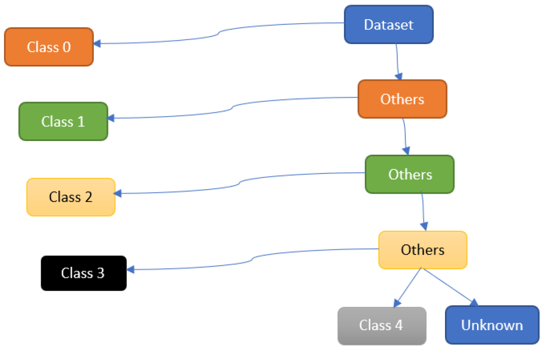
Figure 1: SBC Flowchart

This “divide and conquer strategy” used by SBC can help in better classification of minority data-points, by treating multiple minority classes together, thereby reducing class imbalance. The complexity of the boundary is reduced as it is converted into a series of 2-class problems, which get progressively smaller. Step 8 of the algorithm can be modified to enable the working of SBC with AIDS. The building of progressively smaller models makes SBC efficient compared to OVA and OVO. The training time and model size would be expected to decrease as we move progressively down the hierarchy since the dataset size keeps shrinking. Additionally, this approach makes SBC more extensible than OVA since fewer model retraining cycles may be needed when a new class is added. In principle, only the classifier stages corresponding to the cardinality of the new class and those with more instances are required to be retrained. SBC can incorporate a combination of different base classifiers, enhancing model flexibility. One can incorporate various other base classifiers - from simple DTs to complex models and still retain the interpretability of the model.

III-B Hyperparameter Optimization

Manually defining hyperparameters for each base classifier in SBC will impact its scalability. Additionally, every base classifier is not guaranteed to have the best performance for the same set of hyperparameters. Grid Search coupled with cross-validation is a standard approach for hyperparameter optimization (HPO). However, this method goes through every combination of parameters and performs cross-validation on each of them. This can exponentially increase the time and cost of HPO as the dataset size increases. Halving Grid Search (HGS) [21] is a method for speeding up this process. This is an iterative HPO approach where the number of candidate models reduces exponentially for every iteration by comparing their performance to a threshold score for a metric such as accuracy or mean squared error. Simultaneously, the number of data-points available for each candidate model increases at the same rate [22].

HPO using successive halving still consumes significant time since the number of models required to be trained increases with the number of classes. To address this issue we introduce an additional step along with successive halving. For every base classifier, we bound the hyperparameter search-space using the best values from the previous/parent classification stage. The intuition behind this is that as we go down the hierarchy of classifiers, the models become simpler and, therefore, could use a reduced or bounded HP search-space for HPO. Assuming identical base classifiers, optimal hyperparameters for progressively smaller data subsets/classifiers in SBC may be within a constrained bound of those of the previous parent-level classifier. The bound can be kept as a lower limit or upper limit depending upon the hyperparameter in consideration. For example, if we are tuning the maximum depth of a tree, it would be intuitive to constrain the upper bound as we move towards subsequent models due to the reduction in dataset size. Experiments reported hereafter will demonstrate the efficacy of this approach in reducing HPO time while maintaining competitive performance.

IV Experiments

This section studies the performance of the proposed SBC and its pruned HPO approach through a set of research questions listed below:

1. How does the pruned HPO approach perform compared to standard HPO approaches in SBC?

2. How does SBC perform, when incorporating class imbalance techniques?

3. How does the pruned HPO approach in SBC perform compared to HPO in multi-class classification (MCC)?

4. How does the performance of SBC vary using every HP combination in a pre-defined search space?

5. How does SBC perform on balanced data?

6. How does SBC perform on low-dimensional data?

7. Can we incorporate different base classifiers in SBC? Does it affect the performance of the algorithm?

8. How does SBC perform with non-tree base classifiers?

Two benchmark datasets were used to conduct these experiments. They provide a useful foundation for assessing and contrasting the effectiveness of various network intrusion detection systems. The datasets used were:

1. CICIDS: The CICIDS-2017 dataset consists of benign data, 14 attack classes, 78 features, and 2.47 million records. There was no pre-defined split for train and test in this dataset. This dataset included duplicate rows, missing, negative and infinity values, and underwent considerable data preprocessing. For experimental purposes, a stratified split of 90-10 for training and test data, respectively, was created from the preprocessed dataset. Finally, the training data consists of 2.2 million records, and the test data consists of 247,431 records. This dataset exhibits severe class imbalance, which can be seen by the distribution of all classes in Table I.

2. UNSW: The UNSW-NB15 dataset consists of normal and malicious network traffic created in an emulated environment, for a duration of 31 hours [23]. The dataset comes with a predefined split for training and test data. It consists of nine attack classes. The number of records in the training dataset is 175,341, and the test dataset has 82,332 records, along with 45 features. The distribution of each class is shown in Table II. This dataset was chosen due to its wide range of attack classes, high class imbalance, and being a relatively new dataset. No missing values or duplicate records were found in this dataset. High inter-class overlap is an additional characteristic of this dataset [24].

For all experiments, XGBoost [25] was used as the base classifier, unless specified otherwise, as it exhibits better scalability, high performance and computational efficiency. For experiments requiring performance comparison with MCC, XGBoost using the softmax function was used as the benchmark. Seconds was used as the unit for measuring time in the experiments.

Precision, Recall and F1 were used as the classification metrics for all experiments. For an IDS, the prevention of false negatives for attacks is more important than false positives. An ideal IDS should have a high Recall to identify attacks with better accuracy. However, a high Recall will come at the cost of increased false positives leading to an increase in false alarms. F1-score provides a more robust evaluation of the model. For all experiments, F1-score is taken as the metric to compare model performance followed by Recall.

TABLE I: Class distribution of the CICIDS dataset

Class	Training Data (2,226,870)	Test Data (247,431)
Benign	1,844,452	204,940
DoS Hulk	154,798	17,200
DDoS	115,214	12,802
Portscan	81,737	9082
DoS Goldeneye	9253	1028
FTP-Patator	5340	593
DoS slowloris	4847	538
DoS slowhttptest	4704	523
SSH-Patator	2840	315
Bot	1754	195
Web Attack - Brute Force	1284	143
Web Attack - XSS	587	65
Infiltration	32	4
Web Attack - Sql Injection	18	2
Heartbleed	10	1

TABLE II: Class distribution of the UNSW dataset

Class	Training Data (175,341)	Test Data (82,332)
Normal	56,000	37,000
Generic	40,000	18,871
Exploits	33,393	11,132
Fuzzers	18,184	6062
DoS	12,264	4089
Reconnaisance	10,491	3496
Analysis	2000	677
Backdoor	1746	583
Shellcode	1133	378
Worms	130	44

IV-A How does the pruned HPO approach perform compared to standard HPO approaches in SBC?

As discussed in Section III, hyperparameter optimization (HPO) using HGS was computationally time-consuming in SBC. This led us to introduce hyperparameter search-space pruning as a means of making Halving Grid Search scale for SBC. Another way of speeding up HPO in SBC is by parallelizing the process. The objective of this experiment was to see the impact on the reduction in time for the HPO process using the pruned and parallelized methods. The three methods of HPO are briefly described below:

• Sequential: HPO was carried out in a sequential manner without pruning, starting from the majority-class to the minority class.

• Parallelized: HPO was carried out in a parallelized manner without any pruning. Each core was assigned the task of optimization for an individual classifier. The order of execution did not matter in this case.

• Pruned: The proposed HPO algorithm as described in Section III-B.

For both datasets, the entire training dataset was used for HPO, and the test dataset was used to make predictions. Maximum tree depth, number of tree estimators, and the learning rate were chosen as the hyperparameters for this experiment. These hyperparameters were selected because they significantly affect both model performance and complexity. The search-space for each hyperparameter is shown in the Appendix, in Table A1.

Table III displays the results of this experiment. The difference in time between the sequential and parallelized approaches was significant with the latter producing the same results with a 50% - 55% reduction in total time taken for training and prediction. The difference in time between the parallelized and pruned approach was comparable in the UNSW dataset. The reduction in time was more pronounced in the CICIDS dataset, with a $\approx$60% decrease observed from the parallelized approach. The drop in performance using the pruned approach was $\approx$1%.

TABLE III: Performance comparison of different HPO approaches in SBC

Dataset	HPO Approach	Macro Precision	Macro Recall	Macro F1	Total Time
UNSW	Sequential	0.65	0.7	0.65	2241.64
	Parallelized	0.65	0.7	0.65	1177.7
	Pruned	0.66	0.69	0.64	1147.84
CICIDS	Sequential	0.94	0.88	0.9	24256.71
	Parallelized	0.94	0.88	0.9	10868.33
	Pruned	0.96	0.87	0.89	4370.56

The conclusion drawn from this experiment was that the pruned approach for HPO exhibits competitive performance compared to regular HGS, in significantly less time. This experiment validates our intuition that simpler classifiers (e.g., trees with lesser depth) might suffice towards the lower end of the SBC model structure, and therefore, hyperparameter pruning for SBC enables competitive performance. Given the insights obtained from this experiment, subsequent experiments in this paper used the proposed pruned Halving Grid-Search approach to perform hyperparameter optimization for SBC.

IV-B How does SBC perform, when incorporating class imbalance techniques?

Both the benchmark datasets suffer from severe class imbalance. The objective of this experiment was to compare the performance of data-driven class imbalance techniques discussed in Section II when incorporated into SBC. The best-performing technique would be used in subsequent experiments. Two different approaches were tested in this experiment:

1. The best set of hyperparameters obtained from the pruned HPO approach in Section IV-A was chosen. Using these hyperparameters across all SBC stages, different class imbalance techniques were applied to the test data.

2. Class imbalance techniques were applied simultaneously with HPO on the training data.

TABLE IV: Approach 1: Class imbalance techniques applied to SBC, using best hyperparameters across all stages

Dataset	Technique	Macro Precision	Macro Recall	Macro F1	Total Time
UNSW	Subagging	0.67	0.63	0.62	41.12
	Sample Weights	0.66	0.62	0.61	30.61
	Undersampling	0.66	0.62	0.61	22.17
	SMOTE	0.65	0.69	0.64	43.85
CICIDS	Subagging	0.86	0.88	0.86	287.66
	Sample Weights	0.88	0.88	0.87	170.15
	Undersampling	0.85	0.87	0.85	64.01
	SMOTE	0.87	0.87	0.87	331.24

The results for the first approach are shown in Table IV. SMOTE was observed to have the best Recall and F1-score for the UNSW dataset. SBC with sample-weights and SMOTE had the highest F1-score for the CICIDS dataset, but the former achieved the same result in half the time as the latter.

TABLE V: Approach 2: Class imbalance techniques with pruned HPO applied to SBC stages

Dataset	Technique	Macro Precision	Macro Recall	Macro F1
UNSW	Subagging	0.63	0.58	0.57
	sample-weights	0.66	0.62	0.61
	Undersampling	0.57	0.57	0.53
	SMOTE	0.45	0.52	0.46
CICIDS	Subagging	0.87	0.87	0.86
	sample-weights	0.88	0.88	0.87
	Undersampling	0.88	0.87	0.87
	SMOTE	0.96	0.83	0.85

The results for the second approach are shown in Table V. All sampling techniques performed poorly in this approach, especially in the UNSW dataset. A plausible explanation for this could be the stochasticity generated by sampling techniques. In the case of SMOTE, the synthetic data points might not have represented the accurate properties of minority classes, leading to incorrect optimization. Undersampling could have resulted in the loss of informative data-points. The classification reports for both approaches using SMOTE are shown in the Appendix, in Tables A2 and A3. The performance of the minority classes was found to be poor in the second approach for the UNSW dataset, compared to the first approach. Another reason for this poor performance could be the inter-class overlap of minority classes, as discussed in Section IV. Class-wise performance for the CICIDS using SMOTE (see Tables A4 and A5 in the Appendix) also revealed a similar trend. The performance of sample-weights was the same in both approaches, giving a high F1-score.

Considering both performance and time consumption, it was found that sample-weights was the most suited data-driven class imbalance technique to be incorporated in SBC. For subsequent experiments, sample-weights were incorporated into the SBC and multi-class classification (MCC) algorithms.

IV-C How does the pruned HPO approach in SBC perform compared to HPO in multi-class classification (MCC)?

The objective of this experiment was to compare the HPO approaches in SBC and MCC. In SBC, the pruned HPO approach from Section IV-A was applied, while the regular HPO approach using HGS was applied to MCC. The parameter search-space and the data for HPO were the same as that used in Section IV-A. Tables VI and VII display the results of this experiment. SBC exhibited competitive or better performance than MCC in significantly less time.

TABLE VI: Performance comparison between SBC with pruned HGS (for HPO) and MCC with regular HGS

Dataset	Macro-Precision		Macro-Recall		Macro-F1
	SBC	MCC	SBC	MCC	SBC	MCC
UNSW	0.66	0.86	0.69	0.69	0.64	0.69
CICIDS	0.96	0.97	0.87	0.82	0.89	0.85

TABLE VII: Comparison of time consumption between SBC with pruned HGS (for HPO) and MCC with regular HGS

Dataset	Total Time
	SBC	MCC
UNSW	882.21	2892.23
CICIDS	4020	4983

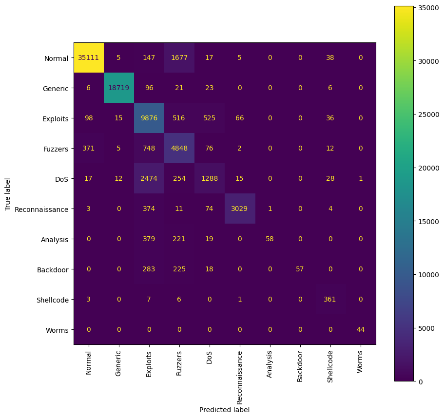
Figure A1: Confusion Matrix for the predictions made using HPO with regular HGS in MCC

The results of this experiment suggested that the efficacy of SBC increases as the datasets become larger. A plausible explanation for this is the presence of adequate exemplars per class, which might have enabled learning. On comparing the classification reports for both SBC and MCC (see Tables VIII and IX respectively), it was observed that the drop in precision for SBC was caused by the misclassification of the minority classes. For further analysis, the confusion matrices for both methods are attached in the Appendix (see Figures A1 and A2). From this experiment, the conclusion reached was that pruned HPO in SBC performs competitively or better than the standard HPO using HGS applied to MCC, but in significantly less time. It also appears that SBC may perform better than MCC for larger datasets.

TABLE VIII: Classwise performance of UNSW dataset using pruned HPO in SBC

Class	Precision	Recall	F1-score
0	0.99	0.94	0.96
1	1.00	0.99	1.00
2	0.85	0.69	0.76
3	0.67	0.73	0.70
4	0.46	0.68	0.55
5	0.92	0.82	0.87
6	0.16	0.66	0.26
7	0.38	0.08	0.14
8	0.48	0.80	0.60
9	0.76	0.50	0.60

TABLE IX: Classwise performance of UNSW dataset using HPO in MCC

Class	Precision	Recall	F1-score
0	0.99	0.95	0.97
1	1.00	0.99	0.99
2	0.69	0.89	0.77
3	0.62	0.80	0.70
4	0.63	0.31	0.42
5	0.97	0.87	0.92
6	0.98	0.09	0.16
7	1.00	0.10	0.18
8	0.74	0.96	0.84
9	0.98	1.00	0.99

IV-D How does the performance of SBC vary using every HP combination in a pre-defined search space?

In the previous experiments, the combination of hyperparameters used for every base classifier was different, as they were found using HPO. This experiment compared the model performance along with the computation time for SBC and multi-class classification for both datasets, across every combination of hyperparameters in a predefined search-space. The range of hyperparameters is the same as used in Section IV-A. The objective of this experiment was to compare the performance between SBC and MCC using an identical set of hyperparameters. The performance of SBC was compared with MCC, both with and without sample-weights. The rationale behind using MCC with and without sample-weights was to understand the difference in the way SBC factors in sample-weights compared to MCC.

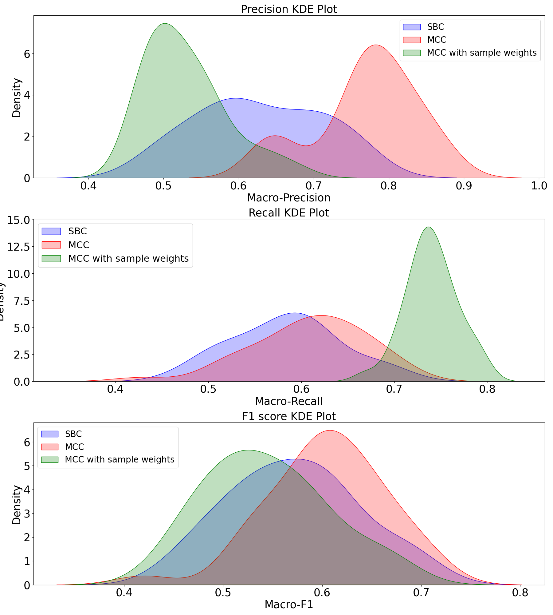
Figure 2: Metric-wise comparison of SBC and MCC for UNSW dataset (All metrics range from 0 to 1)

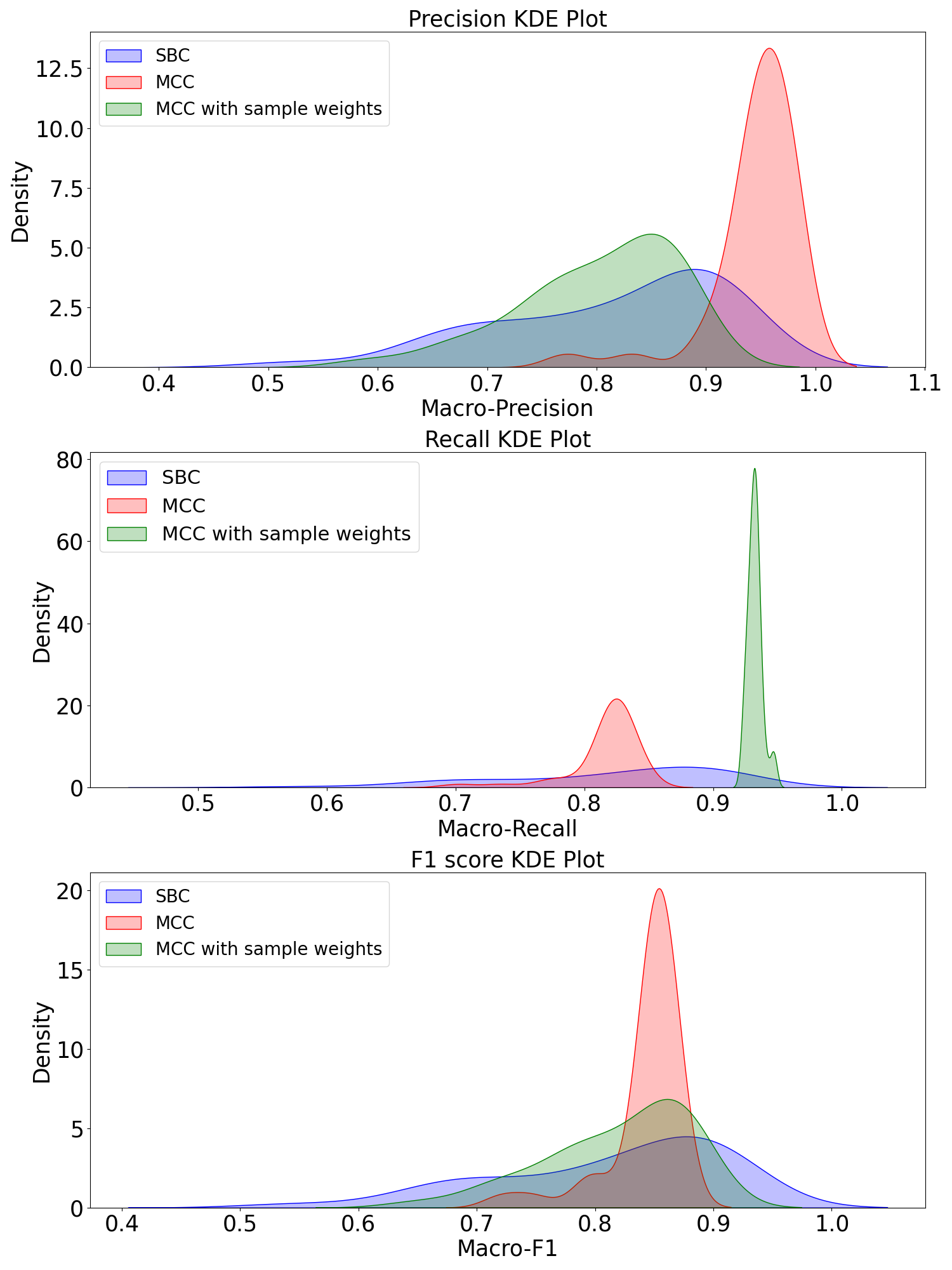
Figure 3: Metric-wise comparison of SBC and MCC for CICIDS dataset (All metrics range from 0 to 1)

Using all combinations from the parameter search-space, 36 models were generated. Figures 2 and 3 display the distribution of the Precision, Recall and F1-scores for the three algorithms across all models. It was observed that MCC without sample-weights had the highest average Precision followed by SBC and MCC without sample-weights. MCC with sample-weights had the highest average Recall by a substantially higher margin in both datasets. The values of all metrics for SBC had a large variance. A plausible reason for this could be due to the use of a fixed set of hyperparameters across all base classifiers. All the base classifiers may not necessarily have optimal performance at the same set of hyperparameters which is why performing HPO is a better alternative. Although SBC did not exhibit the highest average Precision or Recall values, it had high F1-scores. MCC with and without sample weights represent the two extreme ends of classification in imbalanced data. In both datasets, using MCC without sample-weights made the model biased towards the majority-class and increased the instances of classifying an attack to the benign category, which is seen by the low Recall values. The application of sample-weights in MCC increases the sensitivity (Recall) of the model for the minority classes. However, it comes at the cost of a reduction in Precision, resulting in lower F1 values. SBC was able to establish a fair balance between Precision and Recall while applying sample-weights. This resulted in high and varying F1-scores for SBC across different models, as seen in Figures 2 and 3. Tables A6 and A7 in the Appendix show the individual model performance for all three algorithms. An additional observation from these tables was that most of the best-performing models (in terms of F1-score) in SBC had a high learning rate, larger maximum depth and estimators. The plots also suggested that SBC is more sensitive than MCC to HP combinations.

The computation time (training time + prediction time) for both algorithms was also compared in this experiment. Tables A8 and A9 in the Appendix show the computational time for SBC and MCC. Figure 4 compares the computational time against the number of estimators in each model for the CICIDS dataset. For 100 estimators, the computational time between SBC and MCC was similar. As the estimators increased, SBC began to outperform MCC in terms of computational time. This implies that the “divide and conquer” approach of SBC led to a reduction in the model computational time. The time reduction is more pronounced with the increase in the number of estimators.

Figure 4: Comparison of computational time for SBC and MCC vs number of estimators

The inference drawn from this experiment was that SBC exhibits better performance and efficiency, especially with larger datasets. SBC was able to establish a balance between Precision and Recall and enhance the overall model performance. Additionally, the “divide and conquer” approach in SBC led to a significant reduction in computation time.

IV-E How does SBC perform on balanced data?

All previous experiments were carried out on imbalanced data. The objective of this experiment was to understand the efficacy of SBC on balanced data.

Balanced data was created from the existing datasets by extracting a subset of the classes with reasonable balance. From the UNSW dataset, Fuzzers, DoS and Reconnaissance attack classes were selected, while FTP-Patator, DoS slowloris, and DoS Slowhttptest attack classes were chosen from the CICIDS dataset. Since the data was balanced and only a subset of the entire dataset was used for this experiment, the number of estimators was reduced by a factor of 10 to prevent overfitting. Figure 5 compares the performance of SBC and MCC based on F1-scores obtained for all the models. For both datasets, SBC and MCC had similar performance (Figure 5). The results for model performance of SBC and MCC incorporating HPO are shown in Table X. Both algorithms performed similarly in this case as well.

This experiment enabled the conclusion that SBC is able to achieve similar performance as MCC on balanced data. The pruned method of HPO for SBC achieves competitive results using fewer computational resources.

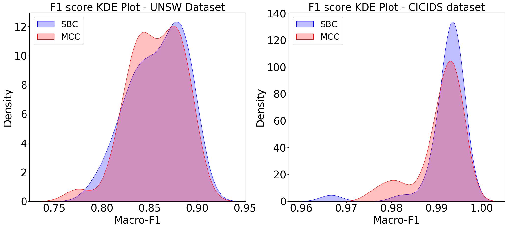
Figure 5: Performance comparison of SBC and MCC on balanced data (Metric ranges from 0 to 1)

TABLE X: Performance comparison of SBC and MCC incorporating HPO on balanced data

Dataset	Macro-Precision		Macro-Recall		Macro-F1
	SBC	MCC	SBC	MCC	SBC	MCC
UNSW	0.90	0.88	0.89	0.88	0.89	0.88
CICIDS	0.99	1.00	0.99	0.99	0.99	0.99

IV-F How does SBC perform on low-dimensional data?

The datasets used in previous experiments have high dimensionality. This experiment aimed to understand the performance of SBC on low-dimensional data.

Principal Component Analysis (PCA) was applied to the IDS datasets to generate low-dimensional data. It enables a comparison with prior results as the data is essentially the same but with a lower dimensional representation. Since this experiment focused on low-dimensional data, the top 9 principal components were retained for use in this experiment. The hyperparameters used were the same as those in Section IV-D. Both algorithms observed a drop in model performance compared to Section IV-D. An explanation for this could be the insufficient number of principal components taken. SBC had a higher F1-score than MCC for both datasets. The results of this experiment aligned with those in IV-D. The performance after incorporating HPO for both algorithms was also compared (see Table XI). SBC had a higher F1-score and Precision, while MCC had a higher Recall. The plausible reasons for these results can be attributed to the similar inferences drawn from IV-D. SBC is able to create greater balance between Precision and Recall, giving a higher F1-score.

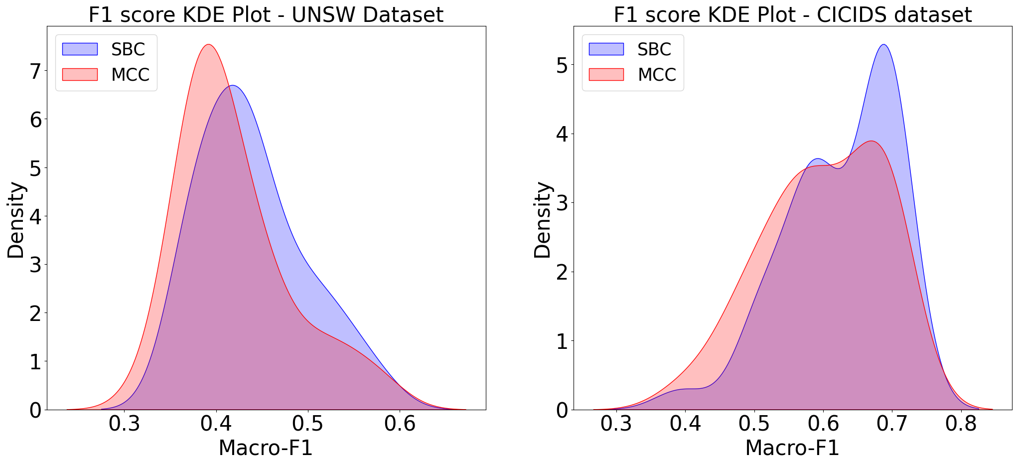
Figure 6: Performance comparison of SBC and MCC on low-dimensional data

TABLE XI: Performance comparison of SBC and MCC with HPO on low-dimensional data

Dataset	Macro-Precision		Macro-Recall		Macro-F1
	SBC	MCC	SBC	MCC	SBC	MCC
UNSW	0.54	0.42	0.55	0.62	0.52	0.40
CICIDS	0.84	0.50	0.65	0.84	0.68	0.55

The conclusion drawn from this experiment was that SBC exhibits better performance than MCC with low-dimensional data. Additionally, when applying HPO, SBC outperformed MCC and produced very similar results to the experiment described in Section IV-D. This experiment further supports the notion that SBC establishes a balance between Precision and Recall.

IV-G Can we incorporate different base classifiers in SBC? Does it affect the performance of the algorithm?

In all previous experiments, XGBoost was used as the base classifier at all stages. In some stages, it may be possible to use different base classifiers to achieve better performance or even competitive performance with less model complexity. One such case is for the minority classes with very few data-points. For such classes, simpler base classifiers such as Decision Trees could be a more efficient choice. The intuition behind this is simpler base classifiers might suffice for minority classes to prevent overfitting. The objective of the experiment was to demonstrate the flexibility of SBC and see if using different base classifiers will change the performance of SBC.

TABLE XII: Performance summary of using variable base classifiers in SBC

Dataset	Secondary Estimator	Macro F1	Total Time
UNSW	Decision Tree	0.6 $\pm$ 0.05	34.14 $\pm$ 6.46
	KNN	0.55 $\pm$ 0.04	34.49 $\pm$ 6.45
CICIDS	Decision Tree	0.88 $\pm$ 0.05	148.96 $\pm$ 34.07
	KNN	0.88 $\pm$ 0.04	151.55 $\pm$ 35.35

Two models were constructed for each dataset using two secondary base classifiers - Decision Tree and K-Nearest Neighbors (KNN). XGBoost was used as the primary base classifier as initial classes. In the UNSW dataset, the last 2 XGBoost models were replaced with KNN and Logistic Regression, while the same was done for the last 3 classes in the CICIDS dataset. The results for this experiment are shown in Table XII. Both models produce similar results in the same time. Comparing the results to the average results of SBC in Section IV-D, the performance and computational time were comparable for both models.

The flexibility of using multiple estimators was demonstrated through this experiment. Although Decision Tree and KNN were used, other algorithms such as Support Vector Machines and Logistic Regression can also be used. The use of simpler models in minority classes can reduce the model complexity and save computational resources.

IV-H How does SBC perform with non-tree base classifiers?

In most prior experiments, tree-based models were used as the base classifiers in SBC. The motivation behind using them was their better performance than non-tree models and exhibiting better interpretability and explainability. However, there might be cases where non-tree models might be preferred to reduce model complexity. In order to analyse the performance of SBC with such models, K-Nearest Neighbors (KNN) and Logistic Regression were taken as the base classifiers for all stages, and the performance was compared to the corresponding KNN and Logistic Regression models in MCC. SVM was not chosen as part of this experiment due to its relatively high complexity while training with large datasets [26].

TABLE XIII: Performance summary of MCC and SBC using KNN as base classifiers

Dataset	Macro F1		Total Time
	SBC	MCC	SBC	MCC
UNSW	0.75$\pm$0.01	0.73$\pm$0.08	473.49$\pm$14.3	9.29$\pm$0.04
CICIDS	0.74$\pm$0.01	0.7$\pm$0.01	5821.3$\pm$12.48	239.02$\pm$0.89

TABLE XIV: Performance summary of MCC and SBC using Logistic Regression as base classifiers

Dataset	Macro F1		Total Time
	SBC	MCC	SBC	MCC
UNSW	0.39$\pm$0.02	0.36$\pm$0.01	11.57$\pm$3.16	32.29$\pm$15.9
CICIDS	0.36$\pm$0.03	0.63$\pm$0.03	52.91$\pm$23.67	379.94$\pm$195.23

For both KNN and Logistic Regression, 4 models each were constructed and the summary of the results are shown in Tables XIII and XIV. For KNN, SBC performed better than MCC in all models but at the cost of a higher computational time, due to the complexity of finding nearest neighbors for each point. This can be offset by using suitable data structures and/or approximate nearest neighbor techniques. The average inference time for SBC was 5821 seconds for the CICIDS dataset and 473 seconds for the UNSW dataset. For MCC, the average inference times were 238 seconds and 9 seconds, respectively. The increased computational overhead during the inference phase increased the total time for model training and predictions. Detailed results for this experiment are shown in the Appendix, in Table A10. In the prediction phase, every data-point has to pass through each base classifier until a positive classification is obtained; this can increase the computational overhead. Combining this overhead with the computationally expensive nature of KNN can lead to a larger training and prediction time. For Logistic Regression, SBC performed poorly on the CICIDS dataset compared to MCC. For the UNSW dataset, the performance of both algorithms was the same, but the time consumption for SBC was much lower. For Logistic Regression, the common observation between both datasets was the significant reduction in total time consumption for SBC. Detailed results for this part of the experiment are shown in Table A11, in the Appendix.

The conclusion drawn from this experiment was that the computational time for SBC is influenced by the base classifier being used. By comparing results obtained from this experiment and in Section IV-G, computationally demanding models like KNN might be better suited towards working with only the minority classes in SBC due to its nature of increasing computational overhead.

V Conclusion

This paper presented Sequential Binary Classification as a structural approach of One-vs-All-Others (OVAO) binarization to address the issue of class imbalance in multi-class classification. SBC leverages the cardinality of classes to design a model. The algorithm enables flexibility and interpretability by using suitable base classifiers at different stages. It also has improved efficiency compared to other binarization techniques like OVA and OVO, as it allows the incorporation of progressively smaller models. The intuition behind SBC is that a boundary that separates two classes is easier to find than an n-class boundary. A pruned HPO approach for SBC is also proposed which leverages the class order to reduce the hyperparameter search-space in a progressive manner, making HPO more scalable and efficient in SBC. The experiments carried out on benchmark network intrusion detection datasets demonstrated SBC as an effective solution to address the issue of class imbalance in multi-class classifications.

The appendix contains further results to enhance the analysis of all the experiments.

TABLE A1: Hyperparameter search-space used for all the experiments

Hyperparameter	Values
Maximum depth	[2, 3, 5]
Number of estimators	[100, 200, 300, 400]
Learning rate	[0.1, 0.2, 0.3]

TABLE A2: Class-wise performance of SMOTE in UNSW dataset, using best hyperparameters across all stages

Class	Precision	Recall	F1-score
0	0.99	0.94	0.96
1	1.00	0.99	1.00
2	0.79	0.74	0.77
3	0.65	0.75	0.70
4	0.46	0.53	0.49
5	0.94	0.81	0.87
6	0.16	0.53	0.25
7	0.37	0.08	0.13
8	0.45	0.83	0.58
9	0.68	0.68	0.68

TABLE A3: Class-wise performance of SMOTE in UNSW dataset, with pruned HPO applied to all stages

Class	Precision	Recall	F1-score
0	0.97	0.83	0.90
1	1.00	0.96	0.98
2	0.75	0.62	0.68
3	0.41	0.65	0.50
4	0.36	0.58	0.44
5	0.74	0.82	0.78
6	0.15	0.47	0.23
7	0.16	0.05	0.08
8	0.25	0.61	0.35
9	0.04	0.14	0.07

TABLE A4: Class-wise performance of SMOTE in CICIDS dataset, using best hyperparameters across all stages

Class	Precision	Recall	F1-score
0	1.00	1.00	1.00
1	0.99	1.00	1.00
2	1.00	1.00	1.00
3	0.99	1.00	0.99
4	0.99	1.00	0.99
5	1.00	1.00	1.00
6	0.99	0.99	0.99
7	0.98	0.99	0.98
8	0.96	0.99	0.98
9	0.48	0.67	0.56
10	0.80	0.53	0.64
11	0.39	0.69	0.50
12	1.00	0.75	0.86
13	0.50	0.50	0.50
14	1.00	1.00	1.00

TABLE A5: Class-wise performance of SMOTE in CICIDS dataset, with pruned HPO applied to all stages

Class	Precision	Recall	F1-score
0	1.00	1.00	1.00
1	1.00	1.00	1.00
2	1.00	1.00	1.00
3	0.99	1.00	0.99
4	1.00	0.99	0.99
5	1.00	1.00	1.00
6	0.99	0.99	0.99
7	0.98	0.99	0.98
8	0.99	0.97	0.98
9	0.92	0.35	0.51
10	0.71	1.00	0.83
11	0.86	0.09	0.17
12	1.00	0.50	0.67
13	1.00	0.50	0.67
14	1.00	1.00	1.00

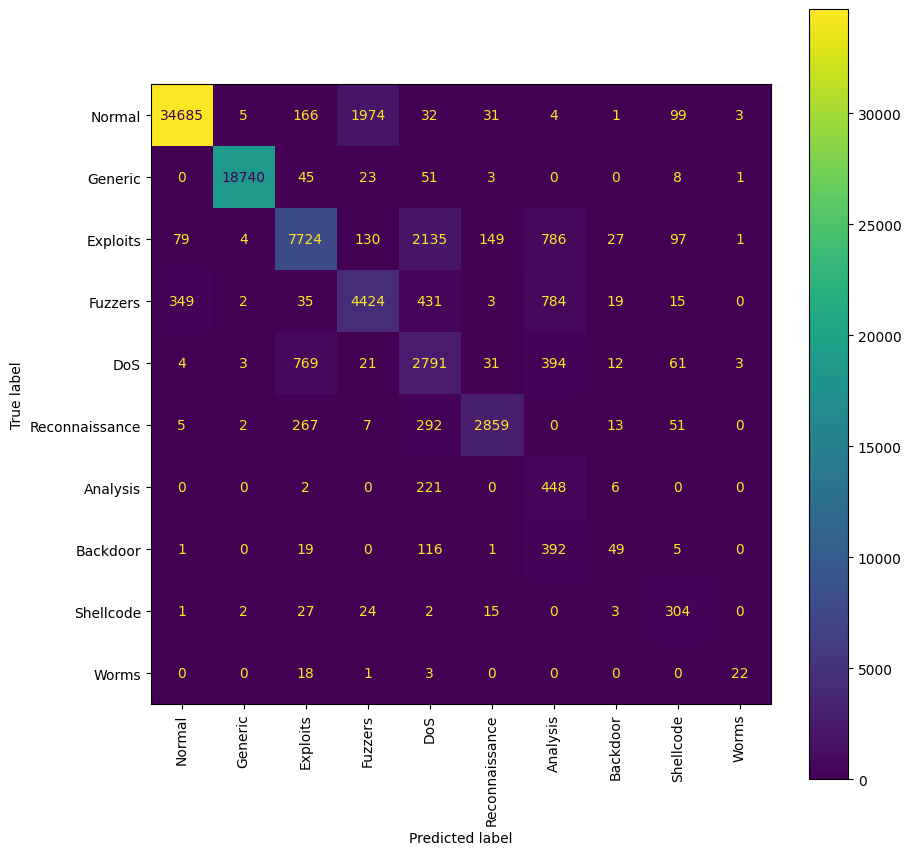
Figure A2: Confusion Matrix for the predictions made using pruned HPO in SBC

TABLE A6: Comparison of the performance of SBC and MCC across a predefined hyperparameter search-space - UNSW dataset

Number	Macro-Precision			Macro-Recall			Macro-F1
	SBC	MCC	MCC (with sample-weights)	SBC	MCC	MCC (with sample-weights)	SBC	MCC	MCC (with sample-weights)
1	0.48	0.63	0.46	0.47	0.43	0.67	0.45	0.42	0.43
2	0.49	0.65	0.47	0.50	0.51	0.70	0.47	0.52	0.45
3	0.52	0.65	0.47	0.50	0.54	0.71	0.48	0.54	0.47
4	0.59	0.72	0.48	0.56	0.55	0.72	0.54	0.55	0.48
5	0.56	0.65	0.47	0.57	0.51	0.71	0.53	0.52	0.47
6	0.60	0.77	0.49	0.57	0.58	0.73	0.55	0.58	0.50
7	0.62	0.77	0.50	0.59	0.60	0.73	0.57	0.59	0.52
8	0.62	0.77	0.51	0.59	0.62	0.74	0.57	0.60	0.53
9	0.60	0.76	0.51	0.54	0.59	0.74	0.52	0.59	0.52
10	0.69	0.79	0.54	0.61	0.62	0.75	0.60	0.62	0.56
11	0.70	0.82	0.55	0.62	0.65	0.76	0.61	0.65	0.58
12	0.72	0.82	0.57	0.63	0.66	0.76	0.63	0.65	0.60
13	0.49	0.64	0.47	0.50	0.52	0.70	0.47	0.53	0.46
14	0.53	0.72	0.48	0.51	0.56	0.72	0.49	0.55	0.49
15	0.59	0.76	0.49	0.57	0.58	0.73	0.55	0.58	0.51
16	0.59	0.76	0.50	0.58	0.60	0.73	0.56	0.59	0.52
17	0.60	0.76	0.49	0.58	0.58	0.72	0.55	0.58	0.50
18	0.58	0.76	0.52	0.54	0.61	0.74	0.53	0.60	0.54
19	0.65	0.79	0.53	0.60	0.63	0.74	0.59	0.62	0.56
20	0.67	0.80	0.55	0.61	0.64	0.75	0.60	0.63	0.57
21	0.69	0.80	0.54	0.61	0.63	0.75	0.60	0.62	0.56
22	0.72	0.83	0.57	0.63	0.66	0.76	0.63	0.66	0.60
23	0.75	0.85	0.60	0.67	0.68	0.78	0.67	0.68	0.63
24	0.76	0.86	0.64	0.68	0.69	0.79	0.68	0.69	0.66
25	0.56	0.65	0.47	0.55	0.53	0.71	0.53	0.53	0.47
26	0.52	0.76	0.49	0.51	0.58	0.73	0.50	0.58	0.51
27	0.54	0.77	0.51	0.53	0.61	0.74	0.51	0.60	0.53
28	0.63	0.77	0.52	0.59	0.62	0.74	0.58	0.61	0.54
29	0.56	0.76	0.51	0.53	0.60	0.73	0.51	0.60	0.52
30	0.65	0.79	0.54	0.59	0.63	0.74	0.59	0.62	0.56
31	0.67	0.81	0.56	0.61	0.65	0.75	0.61	0.64	0.58
32	0.69	0.82	0.57	0.62	0.66	0.76	0.62	0.65	0.59
33	0.70	0.81	0.56	0.62	0.66	0.76	0.61	0.65	0.59
34	0.75	0.85	0.60	0.67	0.68	0.78	0.66	0.68	0.63
35	0.75	0.87	0.64	0.69	0.70	0.79	0.69	0.70	0.66
36	0.77	0.88	0.68	0.71	0.71	0.80	0.70	0.71	0.68

TABLE A7: Comparison of the performance of SBC and MCC across a predefined hyperparameter search-space - CICIDS dataset

Number	Macro-Precision			Macro-Recall			Macro-F1
	SBC	MCC	MCC (with sample-weights)	SBC	MCC	MCC (with sample-weights)	SBC	MCC	MCC (with sample-weights)
1	0.52	0.77	0.59	0.57	0.70	0.94	0.55	0.72	0.65
2	0.64	0.91	0.67	0.67	0.77	0.95	0.64	0.79	0.71
3	0.67	0.97	0.71	0.71	0.81	0.93	0.68	0.84	0.74
4	0.68	0.98	0.75	0.71	0.82	0.93	0.70	0.85	0.77
5	0.70	0.83	0.69	0.70	0.74	0.93	0.68	0.75	0.72
6	0.73	0.97	0.76	0.76	0.83	0.94	0.74	0.86	0.78
7	0.82	0.98	0.78	0.85	0.84	0.94	0.83	0.86	0.81
8	0.84	0.96	0.82	0.86	0.84	0.94	0.85	0.87	0.84
9	0.77	0.90	0.79	0.78	0.79	0.93	0.77	0.80	0.80
10	0.86	0.96	0.86	0.87	0.82	0.93	0.86	0.85	0.87
11	0.91	0.95	0.87	0.90	0.83	0.93	0.90	0.85	0.88
12	0.91	0.94	0.87	0.90	0.84	0.93	0.90	0.87	0.88
13	0.65	0.91	0.67	0.68	0.77	0.95	0.66	0.80	0.71
14	0.68	0.98	0.75	0.71	0.82	0.93	0.69	0.85	0.77
15	0.77	0.98	0.77	0.82	0.82	0.93	0.79	0.85	0.79
16	0.80	0.97	0.80	0.82	0.82	0.93	0.81	0.85	0.82
17	0.77	0.98	0.76	0.79	0.82	0.93	0.78	0.85	0.78
18	0.90	0.97	0.82	0.83	0.82	0.93	0.85	0.85	0.84
19	0.89	0.95	0.84	0.90	0.83	0.93	0.89	0.85	0.85
20	0.89	0.94	0.84	0.90	0.83	0.93	0.89	0.86	0.86
21	0.89	0.97	0.86	0.87	0.82	0.93	0.86	0.85	0.87
22	0.91	0.95	0.87	0.90	0.83	0.92	0.90	0.86	0.87
23	0.91	0.94	0.87	0.89	0.83	0.92	0.89	0.86	0.88
24	0.91	0.94	0.88	0.90	0.83	0.93	0.90	0.86	0.88
25	0.74	0.98	0.73	0.77	0.81	0.93	0.75	0.84	0.76
26	0.69	0.98	0.77	0.71	0.82	0.93	0.70	0.85	0.79
27	0.82	0.97	0.80	0.83	0.82	0.93	0.82	0.85	0.82
28	0.84	0.95	0.83	0.83	0.83	0.93	0.83	0.86	0.85
29	0.82	0.98	0.79	0.84	0.82	0.94	0.82	0.85	0.81
30	0.89	0.95	0.84	0.88	0.83	0.93	0.88	0.86	0.86
31	0.91	0.94	0.84	0.90	0.84	0.93	0.91	0.87	0.86
32	0.91	0.94	0.85	0.90	0.82	0.93	0.90	0.85	0.86
33	0.91	0.94	0.87	0.87	0.81	0.93	0.89	0.84	0.87
34	0.91	0.94	0.88	0.90	0.83	0.93	0.90	0.86	0.88
35	0.91	0.94	0.88	0.90	0.83	0.93	0.90	0.86	0.89
36	0.91	0.94	0.88	0.91	0.83	0.92	0.91	0.86	0.89

TABLE A8: Comparison of the computation time of SBC and MCC across a predefined hyperparameter search-space - UNSW dataset

Number	Maximum Depth	Estimators	Learning Rate	Training Time		Inference Time		Total Time
				SBC	MCC	SBC	MCC	SBC	MCC
1	2	100	0.1	8.71	5.40	10.97	0.18	19.68	5.50
2	2	200	0.1	16.58	10.23	9.43	0.33	26.00	10.41
3	2	300	0.1	19.57	14.68	10.04	0.49	29.61	14.91
4	2	400	0.1	24.82	19.50	10.19	0.61	35.00	19.81
5	3	100	0.1	9.84	6.20	9.92	0.25	19.76	6.34
6	3	200	0.1	16.01	11.67	9.98	0.48	25.99	11.94
7	3	300	0.1	21.59	17.19	10.10	0.73	31.69	17.57
8	3	400	0.1	27.37	22.43	10.24	0.96	37.61	22.93
9	5	100	0.1	11.93	7.63	9.79	0.42	21.72	7.88
10	5	200	0.1	19.15	15.04	10.21	0.87	29.36	15.54
11	5	300	0.1	26.95	21.54	10.57	1.34	37.51	22.29
12	5	400	0.1	34.49	28.14	11.00	1.83	45.49	29.14
13	2	100	0.2	8.66	5.16	9.82	0.20	18.48	5.26
14	2	200	0.2	14.49	14.80	9.51	0.35	24.00	14.98
15	2	300	0.2	19.53	14.34	9.64	0.51	29.18	14.59
16	2	400	0.2	24.75	19.00	9.89	0.68	34.63	19.32
17	3	100	0.2	9.92	5.87	9.85	0.27	19.77	6.03
18	3	200	0.2	15.86	16.83	10.26	0.53	26.12	17.10
19	3	300	0.2	21.42	16.29	9.76	0.79	31.17	16.69
20	3	400	0.2	27.33	27.94	10.85	1.01	38.18	28.48
21	5	100	0.2	11.49	7.37	9.90	0.46	21.39	7.64
22	5	200	0.2	18.82	13.86	10.41	0.93	29.23	14.37
23	5	300	0.2	26.56	20.46	10.98	1.41	37.54	21.22
24	5	400	0.2	33.94	36.11	11.72	1.89	45.66	37.11
25	2	100	0.3	8.64	5.09	9.56	0.19	18.21	5.18
26	2	200	0.3	14.02	9.74	10.05	0.35	24.06	9.92
27	2	300	0.3	19.06	14.20	9.79	0.50	28.85	14.45
28	2	400	0.3	24.68	18.82	10.20	0.66	34.88	19.15
29	3	100	0.3	9.31	5.82	9.53	0.29	18.83	5.97
30	3	200	0.3	15.34	10.98	9.93	0.53	25.27	11.25
31	3	300	0.3	21.04	16.52	9.97	0.79	31.01	16.92
32	3	400	0.3	27.54	21.87	10.40	1.05	37.94	22.40
33	5	100	0.3	11.06	7.43	9.94	0.49	20.99	7.70
34	5	200	0.3	18.79	14.25	10.75	0.96	29.54	14.77
35	5	300	0.3	26.30	21.33	10.77	1.42	37.07	22.11
36	5	400	0.3	35.08	28.16	11.08	1.90	46.16	29.18

TABLE A9: Comparison of computation time of SBC and MCC across a predefined hyperparameter search-space - CICIDS dataset

Number	Maximum Depth	Estimators	Learning Rate	Training Time		Inference Time		Total Time
				SBC	MCC	SBC	MCC	SBC	MCC
1	2	100	0.1	49.54	51.10	12.62	0.18	62.16	51.28
2	2	200	0.1	82.27	100.42	11.54	0.33	93.81	100.75
3	2	300	0.1	109.62	151.14	12.24	0.49	121.86	151.62
4	2	400	0.1	140.24	199.06	12.45	0.61	152.69	199.67
5	3	100	0.1	57.66	58.13	11.58	0.25	69.24	58.38
6	3	200	0.1	91.89	112.35	11.62	0.48	103.52	112.83
7	3	300	0.1	126.95	170.69	12.48	0.73	139.43	171.42
8	3	400	0.1	168.07	236.38	12.48	0.96	180.55	237.35
9	5	100	0.1	63.85	69.88	11.47	0.42	75.32	70.31
10	5	200	0.1	106.4	126.09	12.28	0.87	118.68	126.96
11	5	300	0.1	148.73	248.63	12.62	1.34	161.35	249.97
12	5	400	0.1	192.79	251.69	13.23	1.83	206.02	253.52
13	2	100	0.2	50.17	57.19	11.65	0.20	61.82	57.39
14	2	200	0.2	79.33	102.29	11.94	0.35	91.27	102.65
15	2	300	0.2	110.99	144.42	12.24	0.51	123.24	144.93
16	2	400	0.2	140.16	218.06	12.61	0.68	152.77	218.75
17	3	100	0.2	56.01	62.88	11.95	0.27	67.97	63.15
18	3	200	0.2	92.15	110.86	12.59	0.53	104.73	111.39
19	3	300	0.2	123.92	164.75	11.88	0.79	135.8	165.54
20	3	400	0.2	156.7	221.46	12.39	1.01	169.09	222.47
21	5	100	0.2	63.73	65.04	11.96	0.46	75.69	65.50
22	5	200	0.2	106.32	134.51	12.6	0.93	118.92	135.44
23	5	300	0.2	147.51	193.08	12.65	1.41	160.15	194.48
24	5	400	0.2	188.62	254.16	13.43	1.89	202.05	256.05
25	2	100	0.3	50.11	56.25	11.87	0.19	61.97	56.44
26	2	200	0.3	79.42	106.62	11.88	0.35	91.31	106.97
27	2	300	0.3	108.87	156.54	12.93	0.50	121.8	157.04
28	2	400	0.3	140.12	212.29	12.82	0.66	152.94	212.95
29	3	100	0.3	56.66	69.39	11.82	0.29	68.48	69.68
30	3	200	0.3	90.63	122.90	11.78	0.53	102.4	123.44
31	3	300	0.3	123.84	175.26	12.39	0.79	136.23	176.05
32	3	400	0.3	157.06	231.48	12.88	1.05	169.94	232.54
33	5	100	0.3	64.78	69.43	11.53	0.49	76.31	69.92
34	5	200	0.3	106.27	126.88	12.58	0.96	118.85	127.84
35	5	300	0.3	146.62	190.38	12.59	1.42	159.22	191.80
36	5	400	0.3	187.39	254.48	13.25	1.90	200.64	256.38

TABLE A10: Performance comparison of SBC and MCC using KNN as base classifiers

Dataset	Neighbors	Macro-Precision		Macro-Recall		Macro-F1		Train Time		Inference Time		Total Time
		SBC	MCC	SBC	MCC	SBC	MCC	SBC	MCC	SBC	MCC	SBC	MCC
UNSW	3	0.76	0.73	0.77	0.71	0.73	0.72	0.39	0.15	475.47	9.15	475.86	9.30
	5	0.76	0.74	0.78	0.72	0.75	0.73	0.42	0.14	487.03	9.13	487.44	9.27
	7	0.76	0.75	0.79	0.72	0.75	0.73	0.37	0.12	453.12	9.14	453.49	9.26
	9	0.76	0.75	0.79	0.72	0.75	0.73	0.41	0.12	476.73	9.22	477.15	9.34
CICIDS	3	0.76	0.76	0.75	0.69	0.75	0.71	1.85	0.77	5830.8	238.04	5832.65	238.81
	5	0.76	0.81	0.73	0.69	0.74	0.71	2.15	0.89	5827.14	239.34	5829.29	240.23
	7	0.80	0.81	0.73	0.69	0.75	0.70	2.12	0.82	5802.89	237.28	5805.01	238.10
	9	0.80	0.79	0.73	0.68	0.75	0.68	2.12	0.79	5816.13	238.14	5818.25	238.93

TABLE A11: Performance comparison of SBC and MCC using Logistic Regression as base classifiers

Dataset	Iterations	Macro-Precision		Macro-Recall		Macro-F1		Train Time		Inference Time		Total Time
		SBC	MCC	SBC	MCC	SBC	MCC	SBC	MCC	SBC	MCC	SBC	MCC
UNSW	100	0.36	0.38	0.37	0.39	0.36	0.36	3.68	13.78	4.46	0.04	8.14	13.82
	200	0.4	0.38	0.41	0.39	0.40	0.36	6.76	26.23	3.20	0.01	9.96	26.24
	300	0.4	0.39	0.41	0.39	0.40	0.37	9.74	38.22	3.15	0.01	12.89	38.23
	400	0.4	0.38	0.41	0.39	0.40	0.36	12.16	50.85	3.14	0.02	15.30	50.87
CICIDS	100	0.31	0.63	0.47	0.59	0.35	0.60	20.24	153.87	5.80	0.12	26.04	153.99
	200	0.31	0.74	0.47	0.61	0.35	0.61	38.40	303.84	4.48	0.09	42.88	303.93
	300	0.31	0.76	0.47	0.63	0.35	0.66	57.38	453.51	4.56	0.23	61.94	453.74
	400	0.40	0.77	0.41	0.62	0.40	0.65	75.45	607.93	5.32	0.18	80.77	608.11

References

- [1] L. Haripriya and M. A. Jabbar, “Role of machine learning in intrusion detection system,” in 2018 second international conference on electronics, communication and aerospace technology (ICECA), pp. 925–929, IEEE, 2018.
- [2] M. Wang, N. Yang, D. H. Gunasinghe, and N. Weng, “On the robustness of ml-based network intrusion detection systems: An adversarial and distribution shift perspective,” Computers, vol. 12, no. 10, p. 209, 2023.
- [3] A. Khraisat, I. Gondal, P. Vamplew, and J. Kamruzzaman, “Survey of intrusion detection systems: techniques, datasets and challenges,” Cybersecurity, vol. 2, no. 1, pp. 1–22, 2019.
- [4] Y. Li, Y. Chai, Y. Hu, and H. Yin, “Review of imbalanced data classification methods,” Control and decision, vol. 34, no. 4, pp. 673–688, 2019.
- [5] N. V. Chawla, K. W. Bowyer, L. O. Hall, and W. P. Kegelmeyer, “Smote: synthetic minority over-sampling technique,” Journal of artificial intelligence research, vol. 16, pp. 321–357, 2002.
- [6] I. Sharafaldin, A. H. Lashkari, and A. A. Ghorbani, “Toward generating a new intrusion detection dataset and intrusion traffic characterization.,” ICISSp, vol. 1, pp. 108–116, 2018.
- [7] A. A. ALFRHAN, R. H. ALHUSAIN, and R. U. Khan, “Smote: Class imbalance problem in intrusion detection system,” in 2020 International Conference on Computing and Information Technology (ICCIT-1441), pp. 1–5, IEEE, 2020.
- [8] J. Lee and K. Park, “Gan-based imbalanced data intrusion detection system,” Personal and Ubiquitous Computing, vol. 25, pp. 121–128, 2021.
- [9] P. Soltanzadeh and M. Hashemzadeh, “Rcsmote: Range-controlled synthetic minority over-sampling technique for handling the class imbalance problem,” Information Sciences, vol. 542, pp. 92–111, 2021.
- [10] P. Bühlmann and B. Yu, “Analyzing bagging,” The annals of Statistics, vol. 30, no. 4, pp. 927–961, 2002.
- [11] M. Jakobs and A. Saadallah, “Explainable adaptive tree-based model selection for time-series forecasting,” in 2023 IEEE International Conference on Data Mining (ICDM), pp. 180–189, IEEE, 2023.
- [12] M. T. Ribeiro, S. Singh, and C. Guestrin, “” why should i trust you?” explaining the predictions of any classifier,” in Proceedings of the 22nd ACM SIGKDD international conference on knowledge discovery and data mining, pp. 1135–1144, 2016.
- [13] S. M. Lundberg and S.-I. Lee, “A unified approach to interpreting model predictions,” Advances in neural information processing systems, vol. 30, 2017.
- [14] B. Mahbooba, M. Timilsina, R. Sahal, and M. Serrano, “Explainable artificial intelligence (xai) to enhance trust management in intrusion detection systems using decision tree model,” Complexity, vol. 2021, pp. 1–11, 2021.
- [15] M. Wang, K. Zheng, Y. Yang, and X. Wang, “An explainable machine learning framework for intrusion detection systems,” IEEE Access, vol. 8, pp. 73127–73141, 2020.
- [16] G. Ke, Q. Meng, T. Finley, T. Wang, W. Chen, W. Ma, Q. Ye, and T.-Y. Liu, “Lightgbm: A highly efficient gradient boosting decision tree,” Advances in neural information processing systems, vol. 30, 2017.
- [17] T. Hastie and R. Tibshirani, “Classification by pairwise coupling,” Advances in neural information processing systems, vol. 10, 1997.
- [18] R. Rifkin and A. Klautau, “In defense of one-vs-all classification,” The Journal of Machine Learning Research, vol. 5, pp. 101–141, 2004.
- [19] J. Fürnkranz, “Round robin classification,” The Journal of Machine Learning Research, vol. 2, pp. 721–747, 2002.
- [20] M. Żak and M. Woźniak, “Performance analysis of binarization strategies for multi-class imbalanced data classification,” in Computational Science–ICCS 2020: 20th International Conference, Amsterdam, The Netherlands, June 3–5, 2020, Proceedings, Part IV 20, pp. 141–155, Springer, 2020.
- [21] F. Pedregosa, G. Varoquaux, A. Gramfort, V. Michel, B. Thirion, O. Grisel, M. Blondel, P. Prettenhofer, R. Weiss, V. Dubourg, et al., “Scikit-learn: Machine learning in python,” the Journal of machine Learning research, vol. 12, pp. 2825–2830, 2011.
- [22] L. Li, K. Jamieson, G. DeSalvo, A. Rostamizadeh, and A. Talwalkar, “Hyperband: A novel bandit-based approach to hyperparameter optimization,” Journal of Machine Learning Research, vol. 18, no. 185, pp. 1–52, 2018.
- [23] N. Moustafa and J. Slay, “Unsw-nb15: a comprehensive data set for network intrusion detection systems (unsw-nb15 network data set),” in 2015 military communications and information systems conference (MilCIS), pp. 1–6, IEEE, 2015.
- [24] Z. Zoghi and G. Serpen, “Unsw-nb15 computer security dataset: Analysis through visualization,” 2021.
- [25] T. Chen and C. Guestrin, “Xgboost: A scalable tree boosting system,” in Proceedings of the 22nd acm sigkdd international conference on knowledge discovery and data mining, pp. 785–794, 2016.
- [26] J. Cervantes, X. Li, W. Yu, and K. Li, “Support vector machine classification for large data sets via minimum enclosing ball clustering,” Neurocomputing, vol. 71, no. 4-6, pp. 611–619, 2008.