Self-Distilled Disentangled Learning for Counterfactual Prediction
Abstract.
The advancements in disentangled representation learning significantly enhance the accuracy of counterfactual predictions by granting precise control over instrumental variables, confounders, and adjustable variables. An appealing method for achieving the independent separation of these factors is mutual information minimization, a task that presents challenges in numerous machine learning scenarios, especially within high-dimensional spaces. To circumvent this challenge, we propose the Self-Distilled Disentanglement framework, referred to as . Grounded in information theory, it ensures theoretically sound independent disentangled representations without intricate mutual information estimator designs for high-dimensional representations. Our comprehensive experiments, conducted on both synthetic and real-world datasets, confirms the effectiveness of our approach in facilitating counterfactual inference in the presence of both observed and unobserved confounders.
1. Introduction
Counterfactual prediction has attracted increasing attention (Alaa and van der Schaar, 2017; Chernozhukov et al., 2013; Glass et al., 2013; Zhou et al., 2023) in recent years due to the rising demands for robust and trustworthy artificial intelligence. Confounders, the common causes of treatments and effects, induce spurious relations between different variables, consequently undermining the distillation of causal relations from associations. Thanks to the rapid development of representation learning, a plethora of methods (Li and Yao, 2022; Yao et al., 2018; Shalit et al., 2017) mitigate the bias caused by the observed confounders via generating balanced representations in the latent space. As for the bias brought by the unobserved confounders, Pearl et al. (2000); Angrist and Imbens (1994); Hartford et al. (2017); Muandet et al. (2020); Lin et al. (2019) propose obtaining an unbiased estimator by regressing outcomes on Instrumental variables (IVs), which are exogenous variables related to treatment and only affect outcomes indirectly via treatment, to break the information flow between unobserved confounders and the treatments.
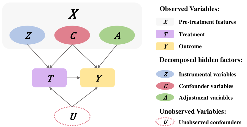
We will further clarify by integrating Figure 1 with a real-world example. Hoxby (2000) examined whether competition among public schools (Treatment T) improves educational quality within districts (Outcome Y). The potential endogeneity of the number of schools in a region arises because both the treatment and the outcome could be influenced by long-term factors (Confounders) specific to the area. Some of these confounders (observed Confounders C) can be measured, such as the level of local economic development. However, other confounders (Unobserved Confounders U) cannot be easily quantified or exhaustively listed, such as certain historical factors. River counts here can serve as a persuasive IV: 1) more rivers can lead to more schools due to transportation (Relevance); 2) yet they are unrelated to teaching quality directly (Exclusivity); 3) the natural attributes of river formation render the counts of the rivers unrelated to the confounders caused by historical factors (Exogeneity).
There are two drawbacks to the existing methods. Firstly, most of them treat all observed features as the observed confounders to block, while only part contributes to the distribution discrepancy of pre-treatment features. Secondly, the prerequisite for IV-based regression methods is to access valid IVs, which have three strict conditions (Relevance, Exclusion, Exogeneity) to satisfy, as shown above, making it a thorny task to find.
Disentangled representation learning (Hassanpour and Greiner, 2019; Wu et al., 2020; Yuan et al., 2022; Cheng et al., 2022b), aiming at decomposing the representations of different underlying factors from the observed features, is showing promise in addressing the flaws above simultaneously. The disentangled factors provide us with a more precise inference route to alleviate the bias brought by the observed confounders. Additionally, one can automatically obtain the representations of the valid IVs to remove the bias led by the unobserved confounders.
The seminar work by Hassanpour and Greiner (2019) introduces disentangled learning to the domain of counterfactual prediction, creatively categorizing observed features into instrumental variables (IVs), confounders, and adjustable variables. However, it does not guarantee the generation of mutually independent representations of these underlying factors. Subsequently, Cheng et al. (2022b); Wu et al. (2020); Yuan et al. (2022) integrate effective mutual information estimators (Cheng et al., 2020) to minimize the mutual information between latent factor representations, aiming to achieve mutually independent latent representations. Nonetheless, the accurate estimation of mutual information between high-dimensional representations remains a persistent challenge (Belghazi et al., 2018; Poole et al., 2019). Inaccurate estimation of mutual information may result in the failure to obtain mutually independent representations of latent factors, thereby compromising the accuracy of counterfactual estimation.
To overcome the defects of previous methods, we propose a novel algorithm for counterfactual prediction named Self-Distilled Disentanglement () to sidestep MI estimation between high-dimensional representations. Specifically, we provide theoretical analysis rooted in information theory to guarantee the mutual independence of diverse underlying factors. Further, we give a solvable form of our method through rigorous mathematical derivation to minimize MI directly rather than explicitly estimating it. Based on the theory put forward, we design a hierarchical distillation framework to kill three birds with one stone: disentangle three independent underlying factors, mitigate the confounding bias, and grasp sufficient supervision information for counterfactual prediction.
Our main contributions are summarized as follows:
-
•
We put forward a theoretically assured solution rooted in information theory for disentanglement to avoid mutual information estimation between high-dimensional representations. It enables the generation of mutually independent representations, thereby adding in the decomposition of diverse underlying factors.
-
•
We provide a tractable form of proposed solution through mathematically rigorous derivation, which rewrites the loss function of disentanglement and fundamentally tackles the difficulty of mutual information estimation between high-dimensional representations.
-
•
We propose a novel self-distilled disentanglement method () for counterfactual prediction. By designing a hierarchical distillation framework, we disentangle IVs and confounders from observational data to mitigate the bias induced by the observed and unobserved confounders at the same time.
-
•
We conduct extensive experiments on synthetic and real-world benchmarks to verify our theoretically grounded strategies. The results demonstrate the effectiveness of our framework on counterfactual prediction compared with the state-of-the-art baselines.
2. Related Work
2.1. Counterfactual Prediction
The main challenge for counterfactual prediction is the existence of confounders. Researchers adopt matching (Rosenbaum and Rubin, 1983), re-weighting (Imbens, 2004), regression (Chipman et al., 2010), representation learning (Shalit et al., 2017; Zhou et al., 2022) to alleviate the confounding bias under the “no hidden confounders” assumption. To relax this unpractical assumption, a few non-parametric or semi-parametric methods utilize special structures among the variables to resolve the bias led by the unobserved confounders. These structures include (1) proxy variables (Veitch et al., 2019, 2020; Louizos et al., 2017; Wu and Fukumizu, 2022); (2) multiple causes (Wang and Blei, 2019; Zhang et al., 2019; Cheng et al., 2022a); (3) instrumental variables. 2SLS (Angrist and Imbens, 1994) is the classical IV method in a linear setting. Singh et al. (2019); Wu et al. (2022a); Xu et al. (2020); Hartford et al. (2017); Lin et al. (2019) adopt advanced machine learning or deep learning algorithms for non-linear scenarios. Another commonly used causal effects estimator using IVs is the control function estimator (CFN) (Wooldridge, 2015; Puli and Ranganath, 2020). These methods require well-predefined IVs or assume all observed features as confounders, which inevitably impairs their generalization to real-world practice. Yuan et al. (2022); Wu et al. (2022b); Li and Yao (2024) aims to generate IVs for downstream IV-based methods rather than focusing on counterfactual prediction.
2.2. Disentangled Representation Learning
Most of the current state-of-the-art disentangled representation learning methods are based on Kingma and Welling (2013), which uses a variational approximation posterior for the inference process of the latent variables. Typical work includes -VAE (Higgins et al., 2017), Factor-VAE (Kim and Mnih, 2018), CEVAE (Louizos et al., 2017) and so on. Another popular solution (Chen et al., 2016; Zou et al., 2020) builds on the basis of Generative Adversarial Networks (Goodfellow et al., 2014). However, these studies are more suitable for the approximate data generation problem and fall short when it comes to estimating causal effects, largely due to the difficulty in training complex generation models.
As the disentanglement of the underlying factors in observed features helps to alleviate confounding bias and improve inference accuracy, Hassanpour and Greiner (2019); Zhang et al. (2021); Wu et al. (2020) design different decomposition regularizers to help the separation of underlying factors. However, these methods fall short in obtaining disentangled representations that are mutually independent, which is a prerequisite for identifying treatment effects. Yuan et al. (2022); Cheng et al. (2022b) employ a cutting-edge mutual information estimator (Cheng et al., 2020) to reduce the mutual information between disentangled representations, thereby promoting independence among the representations of underlying factors. Despite this, the intricacy of mutual information estimation poses a challenge to the accurate separation of latent factors, thereby leaving room for enhancement in counterfactual prediction.
Compared with previous IV-based counterfactual prediction methods, abandons well-predefined IVs but rather decomposes them from pre-treatment variables. Besides, we only impose conditions on variables that are related to confounding bias. Hence, our approach effectively mitigates both unobserved and observed confounding biases concurrently, a feat rarely achieved by previous IV-based counterfactual prediction methods. Compared with generative disentangled methods, rather than generating latent variables, directly disentangles the observed features into three underlying factors by introducing causal mechanisms, which is more efficient and effective. In contrast to preceding causal disentanglement methods, our approach facilitates the generation of mutually independent representations of underlying factors without the need for intricate mutual information estimators. Instead, we fundamentally minimize the mutual information between the representations of underlying factors without explicit estimation, which will be elaborated in Section 4.
3. Problem Setup
As shown in Figure 1, we have observed pre-treatment features , treatment , and outcome in the dataset . is composed of three types of underlying factors:
-
•
Instrumental variable that only directly influences .
-
•
Confounders that directly influences both and .
-
•
Adjustable variable that only directly influences .
Besides these, there are some Unobserved confounders that impede the counterfactual prediction. in this paper are exogenous variables.
According to the d-separation theory (Pearl et al., 2000), , and are mutually independent due to the collider structures and . Thus, encouraging independence among the representations of these underlying factors is essential for advancing their separation. In this paper, we aim to first disentangle mutually independent representations of , , and from , bypassing the explicit estimation of mutual information through theoretical analysis, then propose a unified framework to tackle confounding bias caused by and simultaneously.
Given the above definitions, we present the formal definitions of counterfactual prediction problem, followed by an essential assumption for identification of causal effects adopted in this paper.
Definition 3.1.
Counterfactual Prediction refers to predicting what the outcome would have been for an individual under an intervention (Pearl et al., 2000), i.e.,
| (1) |
where do refers to do-operator proposed by Pearl et al. (2000).
Assuming successful separation of , , and , the sufficient identification results for causal effects under the additive noise assumption in instrumental variable regression were developed by Angrist et al. (1996).
Additive Noise Assumption: the noise from unmeasured confounders is added to the outcomes , i.e.,
| (2) |
4. Methodology
4.1. Theoretical Foundation of Independentizing Underlying Factors
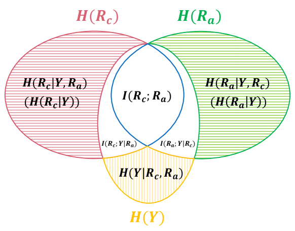
To get the mutually independent representations of underlying factors, an intuitive thought is to minimize the mutual information between the representation of , and , i.e., 111 and differ from and in Figure 1. Our optimization aims to bring and to the states where and can be represented. Initially, and are entangled with non-zero mutual information and thus do not follow the causal relations in Figure 1, as depicted in Figure 2. We introduce constraints to reduce their MI and achieve independence. and , where represents the function of mutual information, during training. However, it is hard due to the notorious difficulty in estimating mutual information in high dimensions, especially for latent embedding optimization (Belghazi et al., 2018; Poole et al., 2019). To circumvent this challenge, we decompose the mutual information between and by leveraging the chain rule of mutual information:
| (3) |
We further inspect the term in Eq (3). Based on the definition of mutual information, we have,
| (4) |
where represents the function of entropy. Intuitively, this conditional mutual information measures the information contained in that is related to but unrelated to . As shown in Figure 1, the only connection between and is that they determine jointly with . If we set up two prediction models from and to Y, respectively, then the mutual information between and is all related to during the training phase. We draw the Venn diagram of mutual information between , and as shown in Figure 2, according to which we have,
| (5) |
With Eq (3), (4) and (5), we have,
| (6) |
Eq (6) transforms the mutual information between two training high-dimensional representations into the subtraction of two mutual information estimators with known labels. To further simplify it, we introduce the following theory:
Theorem 4.1.
Minimizing the mutual information between and is equivalent to:
| (7) |
To find a tractable solution to Eq (7), we derive the following Corollary:
Corollary 4.2.
One of sufficient conditions of minimizing is minimizing the following conditions together:
| (8a) | |||||
| (8b) |
where , represent the predicted distributions of , represents the real distribution of . denotes the KL-divergence.
Detailed proof and formal assertions of Theo.4.1 and Corol.4.2 can be found in the Appendix A.1.1 and A.1.2. Similarly, we can transform minimizing into following:
| (9a) | |||||
| (9b) |
where , represent the predicted distributions of , represents the real distribution of .
Remark: Technically, the optimization of Eq (8a),(8b) can be realized by training prediction networks about . Additionally, we can set up a deep prediction network from , , to and use its supervision information to guide the training of the shallow prediction models. From this perspective, our approach is essentially a self-distillation model. Therefore, we name our method as Self-Distilled Disentanglement, i.e., .
4.2. Self-Distilled Disentanglement Framework
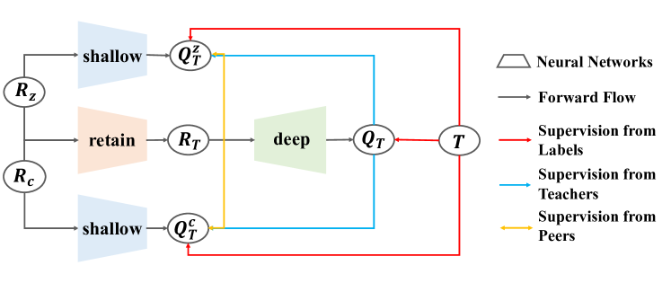
With the theory put forward in section 4.1, we propose a self-distilled framework to disentangle different mutually independent underlying factors. To clarify further, we take the distillation unit for minimizing to illustrate how we employ different sources of supervision information to directly minimize mutual information without explicitly estimating it.
As shown in Figure 3, Retain network represents the neural network for retaining the information from both and . Deep networks and Shallow networks are named based on their relative proximity to and . We set up two Shallow prediction networks from and to , respectively. In addition, to ensure and grasp sufficient information for predicting , we set up a Retain network to concatenate and and store joint information of them for input into a Deep prediction network. To minimize , we deploy distinct sources of supervision information from:
(1) Labels; We use directly to guide the training of deep prediction networks by minimizing the prediction loss . For shallow prediction networks, we reduce and by minimizing prediction loss and .222In practice, only minimizing Eq (9a) and (9b) makes convergence challenging, resulting in unsatisfactory performance. We speculate that this is due to a lack of sufficient supervised information guiding the updating direction of the prediction network for . Therefore, we introduce the minimization of (corresponding loss function to expedite loss convergence.
(2) Teachers; We regard retain and deep prediction networks as a teacher model, which can convey the learned knowledge to help the training of shallow prediction networks. That is, minimizing KL-divergence loss and .
(3) Peers; We diminish the KL-divergence between the distributions of the outputs from the two shallow prediction networks, i.e., . are consequently minimized.
Similarly, we can minimize by establishing corresponding distillation units according to Corol.4.2. In addition, Hassanpour and Greiner (2019) propose to separate from based on . Specifically, for binary treatment setting, they minimize the distribution discrepancy of representations of between the treatment group ( = 1) and the control group ( = 0). The related loss function can be defined as follows:
| (10) |
where function represents the distribution discrepancy of between the treatment and control groups while i refers to the i-th individual. We also provide continuous version of in the Appendix A.2.1.
Mitigating Confounding Bias: With disentangled confounders , the confounding bias induced by can be alleviated by re-weighting the factual loss with the context-aware importance sampling weights (Hassanpour and Greiner, 2019) for each individual . Besides, , the output of the deep prediction network for , can be employed to regress , which helps to mitigate the confounding bias caused by unobserved confounders (Hartford et al., 2017).
The loss function of is thus devised as follows, where can be any functions measuring the differences between two items. , , , are adjustable hyper-parameters. The regularization loss on model weights is to avoid over-fitting.
| (11) |
| Within-Sample | Out-of-Sample | |||||||
| Method | 0-4-4-2-2 | 2-4-4-2-2 | 0-4-4-2-10 | 0-6-2-2-2 | 0-4-4-2-2 | 2-4-4-2-2 | 0-4-4-2-10 | 0-6-2-2-2 |
| DirectRep | 0.037(0.023) | 0.034(0.009) | 0.060(0.014) | 0.043(0.025) | 0.034(0.024) | 0.034(0.013) | 0.060(0.015) | 0.037(0.024) |
| CFR | 0.031(0.014) | 0.032(0.017) | 0.056(0.017) | 0.060(0.019) | 0.027(0.016) | 0.032(0.021) | 0.031(0.024) | 0.054(0.018) |
| DRCFR | 0.058(0.018) | 0.050(0.025) | 0.071(0.020) | 0.066(0.015) | 0.053(0.016) | 0.050(0.023) | 0.071(0.020) | 0.059(0.018) |
| DFL | 3.696(0.034) | 3.702(0.045) | 4.055(0.041) | 3.450(0.030) | 6.796(0.056) | 6.750(0.086) | 7.398(0.051) | 6.393(0.063) |
| DeepIV-Log | 0.569(0.024) | 0.567(0.011) | 0.601(0.011) | 0.531(0.019) | 0.572(0.028) | 0.567(0.016) | 0.601(0.011) | 0.537(0.021) |
| DeepIV-Gmm | 0.466(0.012) | 0.387(0.021) | 0.518(0.012) | 0.437(0.007) | 0.469(0.008) | 0.387(0.021) | 0.517(0.009) | 0.442(0.004) |
| DFIV | 3.947(0.108) | 3.810(0.041) | 4.400(0.134) | 3.644(0.103) | 7.047(0.131) | 6.856(0.093) | 7.749(0.125) | 6.585(0.130) |
| OneSIV | 0.504(0.008) | 0.441(0.063) | 0.569(0.013) | 0.478(0.012) | 0.507(0.009) | 0.441(0.064) | 0.569(0.015) | 0.484(0.014) |
| CBIV | 0.063(0.025) | 0.065(0.032) | 0.049(0.022) | 0.033(0.023) | 0.059(0.024) | 0.067(0.030) | 0.049(0.023) | 0.030(0.017) |
| Ours | 0.010(0.008) | 0.017(0.013) | 0.029(0.019) | 0.014(0.013) | 0.012(0.008) | 0.022(0.017) | 0.029(0.018) | 0.013(0.010) |
| Within-Sample | Out-of-Sample | |||||||
| Method | Twins-0-16-8 | Twins-4-16-8 | Twins-0-16-12 | Twins-0-20-8 | Twins-0-16-8 | Twins-4-16-8 | Twins-0-16-12 | Twins-0-20-8 |
| DirectRep | 0.015(0.007) | 0.009(0.008) | 0.018(0.012) | 0.012(0.007) | 0.023(0.011) | 0.014(0.013) | 0.023(0.016) | 0.014(0.010) |
| CFR | 0.011(0.010) | 0.012(0.008) | 0.017(0.014) | 0.010(0.011) | 0.016(0.008) | 0.019(0.010) | 0.025(0.019) | 0.019(0.014) |
| DRCFR | 0.015(0.016) | 0.008(0.005) | 0.016(0.017) | 0.024(0.017) | 0.020(0.019) | 0.018(0.007) | 0.020(0.009) | 0.028(0.018) |
| DFL | 0.173(0.018) | 0.181(0.014) | 0.169(0.020) | 0.175(0.019) | 0.243(0.136) | 0.252(0.140) | 0.240(0.141) | 0.245(0.145) |
| DeepIV-Log | 0.019(0.010) | 0.017(0.016) | 0.022(0.011) | 0.012(0.007) | 0.028(0.016) | 0.026(0.019) | 0.028(0.018) | 0.018(0.011) |
| DeepIV-Gmm | 0.022(0.004) | 0.016(0.004) | 0.022(0.003) | 0.018(0.004) | 0.017(0.011) | 0.013(0.009) | 0.017(0.011) | 0.013(0.011) |
| DFIV | 0.186(0.014) | 0.185(0.015) | 0.186(0.014) | 0.163(0.023) | 0.257(0.145) | 0.255(0.148) | 0.256(0.144) | 0.227(0.151) |
| OneSIV | 0.015(0.011) | 0.008(0.005) | 0.030(0.017) | 0.017(0.006) | 0.016(0.014) | 0.011(0.007) | 0.025(0.020) | 0.013(0.010) |
| CBIV | 0.024(0.016) | 0.057(0.012) | 0.051(0.038) | 0.037(0.019) | 0.033(0.016) | 0.063(0.017) | 0.057(0.039) | 0.043(0.022) |
| Ours | 0.008(0.006) | 0.007(0.004) | 0.007(0.006) | 0.008(0.006) | 0.012(0.007) | 0.011(0.006) | 0.012(0.006) | 0.011(0.009) |
5. Experiments
5.1. Benchmarks
Due to the absence of counterfactual outcomes in reality, it is challenging to conduct counterfactual prediction on real-world datasets. Previous works (Shalit et al., 2017; Li and Yao, 2022; Wu et al., 2020) synthesize datasets or transform real-world datasets. In this paper, we have conducted multiple experiments on a series of synthetic datasets and a real-world dataset, Twins. The source code of our algorithm is available on GitHub333https://github.com/XinshuLI2022/SDD.
5.1.1. Simulated Datasets
Binary Scenario: Similar to Hassanpour and Greiner (2019)444The difference between our data generation process and that of Hassanpour and Greiner (2019) lies in the introduction of unobserved confounders , in the generation processes of and . Additionally, we categorize IVs into observed and unobserved ones, facilitating comparisons with various baseline algorithms., we generate the synthetic datasets according to the following steps:
-
•
For in , , , , , sample from , where denotes degree identity matrix. Concatenate , , and to constitute the observed covariates matrix . represents the observed IVs, the dimension of which could be set to 0. The setting of is mainly for the comparison of IV-based methods. represents the unobserved confounders.
-
•
Sample treatment variables as following:
(12) where , , , represent the dimension of , , , respectively.
-
•
Sample outcome variables as following:
(13) where represents the dimension of .
5.1.2. Real-World Datasets
Twins: The Twins dataset comprises the records of the twins who were born between 1989-1991 in the USA (Almond et al., 2005). We select 5271 records of same-sex twins who weighed less than 2kg and had no missing features in the records. The heavier twin in twins is assigned with = 1 and the lighter one with = 0. The mortality after one year is the observed outcome. It is reasonable that only part of the features determine the outcome. Therefore, we randomly generate -dimension and choose some features as a combination of , and to create according to the policy in Eq.(12). The rest features will include and some noise naturally. We hide some features in during training to create and treat the rest features in with as .
During training, only , , and will be accessible under any scenario.
| Within-Sample | |||
| Method | Demands-0-1 | Demands-0-5 | Demands-5-1 |
| DirectRep | 472.14(292.68) | 319.27(156.58) | 795.38(304.10) |
| CFR | 1180.26(439.56) | 340.12(175.82) | 1891.91(79.78) |
| DFL | 786.92(122.35) | 1074.71(142.78) | 874.78(103.71) |
| DRCFR | 720.51(195.09) | 451.31(407.55) | 809.04(94.98) |
| DEVAE | >10000 | >10000 | >10000 |
| DeepIV-Gmm | 1774.71(757.98) | 3429.79(438.65) | 2618.72(775.20) |
| DFIV | 862.00(123.71) | 1420.24(257.10) | 909.25(137.05) |
| OneSIV | 2573.15(157.31) | >10000 | 2352.69(125.16) |
| CBIV | 819.52(535.05) | 410.42(241.71) | 2542.58(442.26) |
| Ours | 170.55(6.51) | 216.55(47.11) | 171.07(6.41) |
| Out-of-Sample | |||
| Method | Demands-0-1 | Demands-0-5 | Demands-5-1 |
| DirectRep | 494.47(287.92) | 303.22(144.85) | 768.15(278.24) |
| CFR | 1103.00(362.45) | 326.54(110.31) | 1877.60(119.71) |
| DFL | 736.35(123.44) | 914.08(90.11) | 822.71(65.88) |
| DRCFR | 766.22(188.86) | 498.22(363.25) | 864.21(83.39) |
| DEVAE | >10000 | >10000 | >10000 |
| DeepIV-Gmm | 904.60(618.41) | 2423.33(326.23) | 2405.33(675.40) |
| DFIV | 943.57(188.70) | 1213.27(388.08) | 1050.65(253.38) |
| OneSIV | 2744.87(182.35) | 4243.51(596.10) | 2538.77(147.29) |
| CBIV | 2990.19(735.92) | 316.66(114.89) | 2958.70(614.26) |
| Ours | 183.21(14.18) | 199.44(14.60) | 187.20(16.05) |
5.2. Comparison Methods and Metrics
The baselines can be classified into two categories:
IV-based Methods: DeepIV-Log and DeepIV-Gmm (Hartford et al., 2017), DFIV (Xu et al., 2020), OneSIV (Lin et al., 2019), CBIV (Wu et al., 2022a). These methods need well-predefined IVs . When there is no , i.e., equals 0, we use as for comparison.
Non-IV-based Methods: DirectRep, CFR-Wass (Shalit et al., 2017), DFL (Xu et al., 2020), DRCFR (Hassanpour and Greiner, 2019), CEVAE (Louizos et al., 2017). The latter two also disentangle the hidden/latent factors from observed features.
Metrics: We use the absolute bias of Average Treatment Effect, i.e., , to evaluate the performance of different algorithms in the binary scenario. Formally,
| (14) |
where represents the factual/predicted potential outcome. For continuous scenarios, we take Mean Squared Error () as the evaluation metric. The smaller and are, the better the performance.
5.3. Results
5.3.1. Comparison with the SOTA methods
Binary Scenario: Table 1 shows the performance of on datasets with binary values. ---- represents the data generated with predefined IVs , underlying IVs , underlying confounders , underlying adjustable variables and unobserved confounders . During training, we can only observe , and as a whole . Twins--- denotes the Twins dataset with predefined IVs, observed pre-treatment covariates and unobserved confounders and IVs. For data setting with (Twins---, Twins---, Twins---), there are 12 confounders and IVs, 4 adjustable variables and noises, while for Twins---, we add 4 confounders and IVs in .
We generate 10000 samples for synthetic datasets for training, validation and testing sets, respectively, For the Twins datasets, we randomly choose 5271 samples and split the datasets with the ratio 63/27/10. We perform 10 replications and report the mean and standard deviation of the bias of ATE estimation. Taking the results in 0-4-4-2-2 as a base point for observation, we have the following findings:
-
•
The results of almost all IV-based methods in 0-4-4-2-2 are worse than those in 2-4-4-2-2, demonstrating the performance of IV-based methods is highly dependent on the predefined instrumental variables.
-
•
By comparing the results between 0-4-4-2-2 and 0-4-4-2-10, we find that when there are more unobserved confounders in the dataset, the performance of confounder balancing methods (such as CFR, DRCFR, and DFL) will be poorer, which indicates the necessity of controlling the unobserved confounders.
-
•
If there are fewer confounders in observed features, as we compare 0-4-4-2-2 with 0-2-6-2-2, the performance of confounder balancing methods without disentanglement (such as CFR, DFL) gets impeded, implying the significance of precise confounder control by decomposing underlying factors.
-
•
achieves the best performance among all data settings and is far better than the second-best methods. It proves counterfactual prediction benefits from simultaneously controlling the underlying confounders in observational features and unobserved confounders. The effectiveness of our disentanglement theory and hierarchical self-distillation framework is thus validated. The results in all Twins datasets are consistent with these findings.
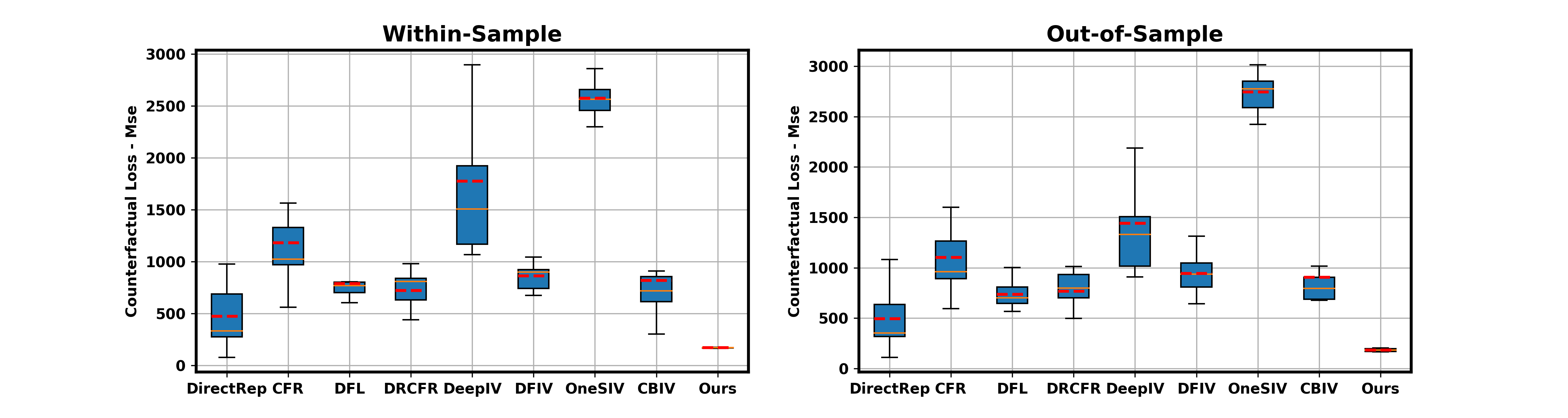
Continuous Scenario: Following Wu et al. (2022a), we use Demand-- to denote different data setting in Demands datasets. Demand-0-1 represents the original Demand dataset defined in Hartford et al. (2017). The in Demand-- denotes the extra information from instrumental variables while the indicates the information increasing from instrumental variables and underlying confounders together on the basis of Demand-0-1. We only present the results on Demand-0-1 with box plots as shown in Figure 4, where we omit the results of CEVAE as its is beyond 10000.
The IV-based methods perform worse than the non-IV-based ones under the continuous scenario. This result indicates that confounding bias from the treatment regression stage is a critical problem in IV-based methods, underscoring the necessity of decomposing from observed variables and thereby correcting for confounding bias caused by , coinciding with the findings under the binary scenario. We notice that DRCFR, which performs well on discrete datasets, suffers significantly on the Demand-0-1, reflecting the limitations of their disentanglement theory under the continuous scenario. Among all the baselines, achieves the best and most stable performance on all Demands Datasets, demonstrating the generalizability of on various types of datasets.
The detailed experimental results on all Demands datasets are provided in the Table 2. It can be seen that whether adding the information of instrumental variables (Demands-5-1) or increasing the information of confounders (Demands-0-5), our algorithm performs far better than all the baseline, which proves the efficiency and generalizability of our method.
| Within-Sample | 0-4-4-2-2 | 2-4-4-2-2 | 0-4-4-2-10 | 0-6-2-2-2 | Twins-0-16-8 | Twins-4-16-8 | Twins-0-16-12 | Twins-0-20-8 |
|---|---|---|---|---|---|---|---|---|
| CLUB | 0.514(0.005) | 0.513(0.006) | 0.563(0.006) | 0.481(0.006) | 0.020(0.009) | 0.029(0.008) | 0.024(0.007) | 0.023(0.005) |
| Ours | 0.010(0.008) | 0.017(0.013) | 0.029(0.019) | 0.014(0.013) | 0.008(0.006) | 0.007(0.004) | 0.007(0.006) | 0.008(0.006) |
| Out-of-Sample | 0-4-4-2-2 | 2-4-4-2-2 | 0-4-4-2-10 | 0-6-2-2-2 | Twins-0-16-8 | Twins-4-16-8 | Twins-0-16-12 | Twins-0-20-8 |
| CLUB | 0.517(0.004) | 0.513(0.006) | 0.563(0.004) | 0.487(0.005) | 0.016(0.013) | 0.026(0.009) | 0.021(0.012) | 0.018(0.010) |
| Ours | 0.012(0.008) | 0.022(0.017) | 0.029(0.018) | 0.013(0.010) | 0.012(0.007) | 0.011(0.006) | 0.012(0.006) | 0.011(0.009) |
| Datasets | Within-Sample | Out-of-Sample | ||||||
|---|---|---|---|---|---|---|---|---|
| Twins-0-16-8 | 0.027(0.012) | 0.025(0.007) | 0.021(0.007) | 0.008(0.006) | 0.022(0.011) | 0.020(0.011) | 0.018(0.010) | 0.012(0.007) |
| Twins-4-16-8 | 0.067(0.078) | 0.022(0.005) | 0.024(0.005) | 0.008(0.005) | 0.059(0.076) | 0.017(0.012) | 0.019(0.012) | 0.009(0.006) |
| Twins-0-16-12 | 0.113(0.110) | 0.027(0.005) | 0.024(0.005) | 0.007(0.006) | 0.111(0.109) | 0.022(0.011) | 0.019(0.012) | 0.012(0.006) |
| Twins-0-20-8 | 0.031(0.010) | 0.020(0.004) | 0.023(0.006) | 0.008(0.006) | 0.026(0.013) | 0.015(0.009) | 0.018(0.012) | 0.011(0.009) |
| Syn-0-4-4-2-2 | 0.519(0.005) | 0.513(0.005) | 0.513(0.004) | 0.010(0.008) | 0.522(0.004) | 0.517(0.004) | 0.516(0.004) | 0.012(0.008) |
| Syn-2-4-4-2-2 | 0.517(0.007) | 0.513(0.007) | 0.513(0.007) | 0.017(0.013) | 0.517(0.006) | 0.512(0.007) | 0.513(0.006) | 0.022(0.017) |
| Syn-0-4-4-2-10 | 0.569(0.005) | 0.565(0.004) | 0.565(0.005) | 0.029(0.019) | 0.568(0.004) | 0.565(0.004) | 0.564(0.004) | 0.029(0.018) |
| Syn-0-6-2-2-2 | 0.486(0.004) | 0.483(0.004) | 0.483(0.004) | 0.015(0.013) | 0.492(0.005) | 0.489(0.005) | 0.489(0.005) | 0.013(0.010) |
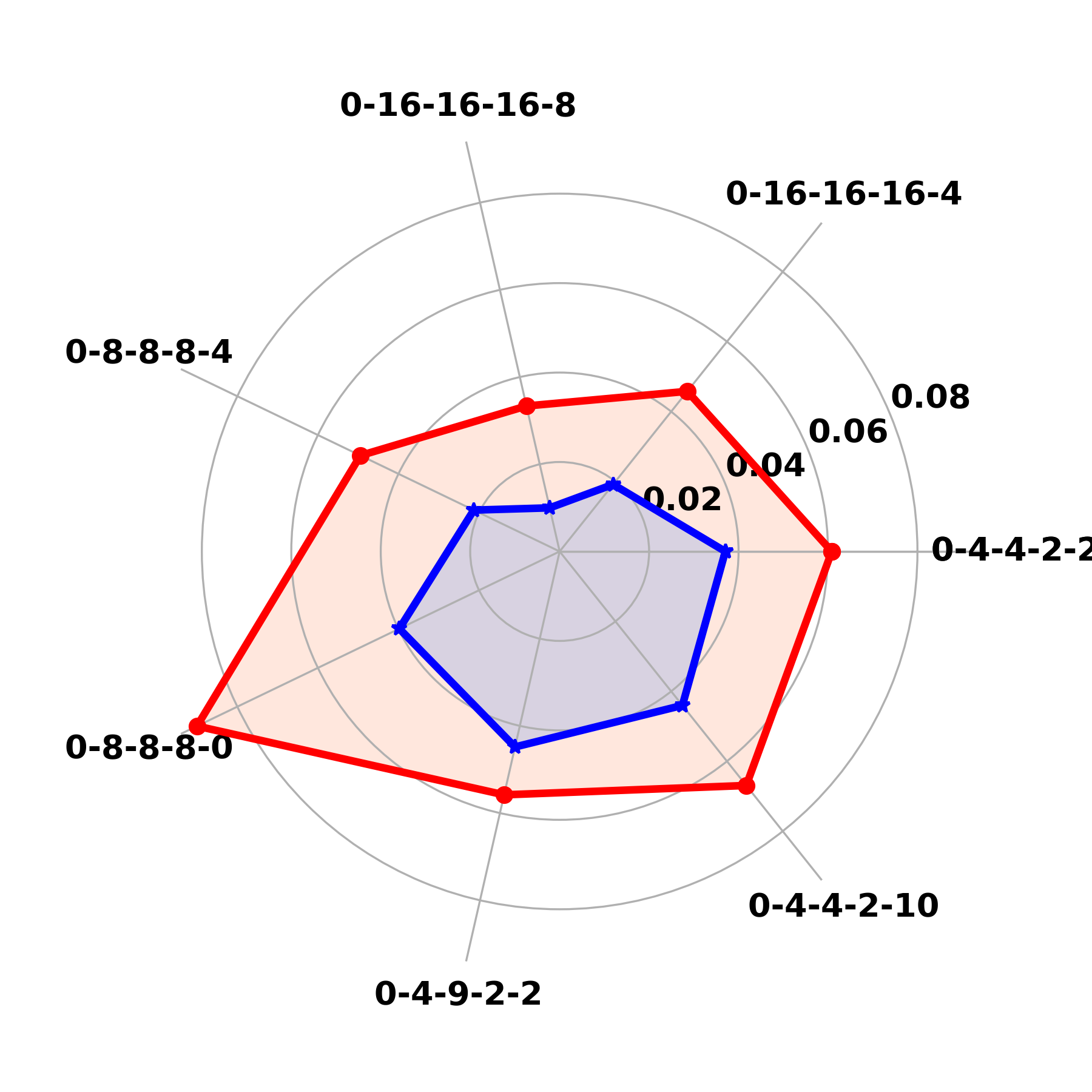
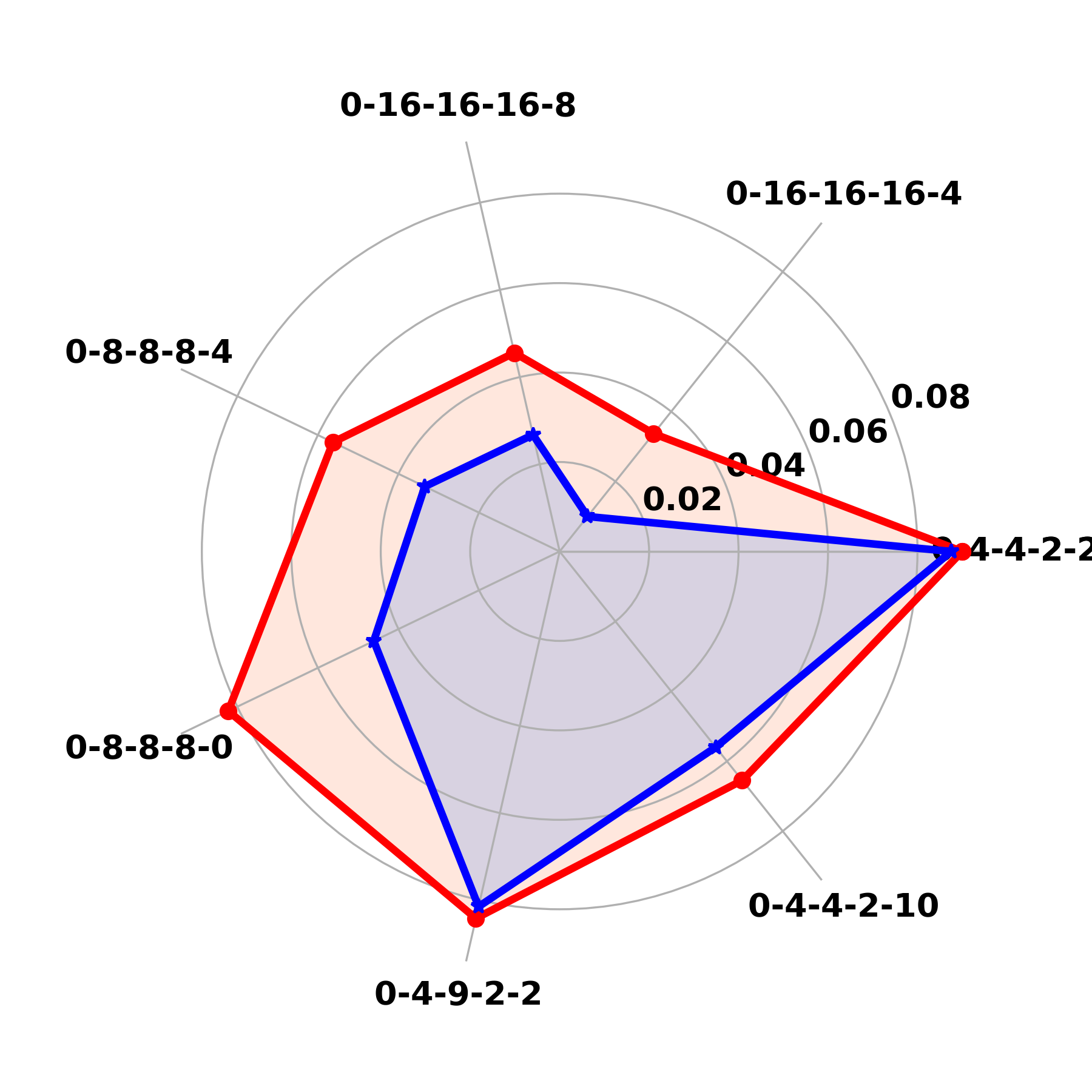
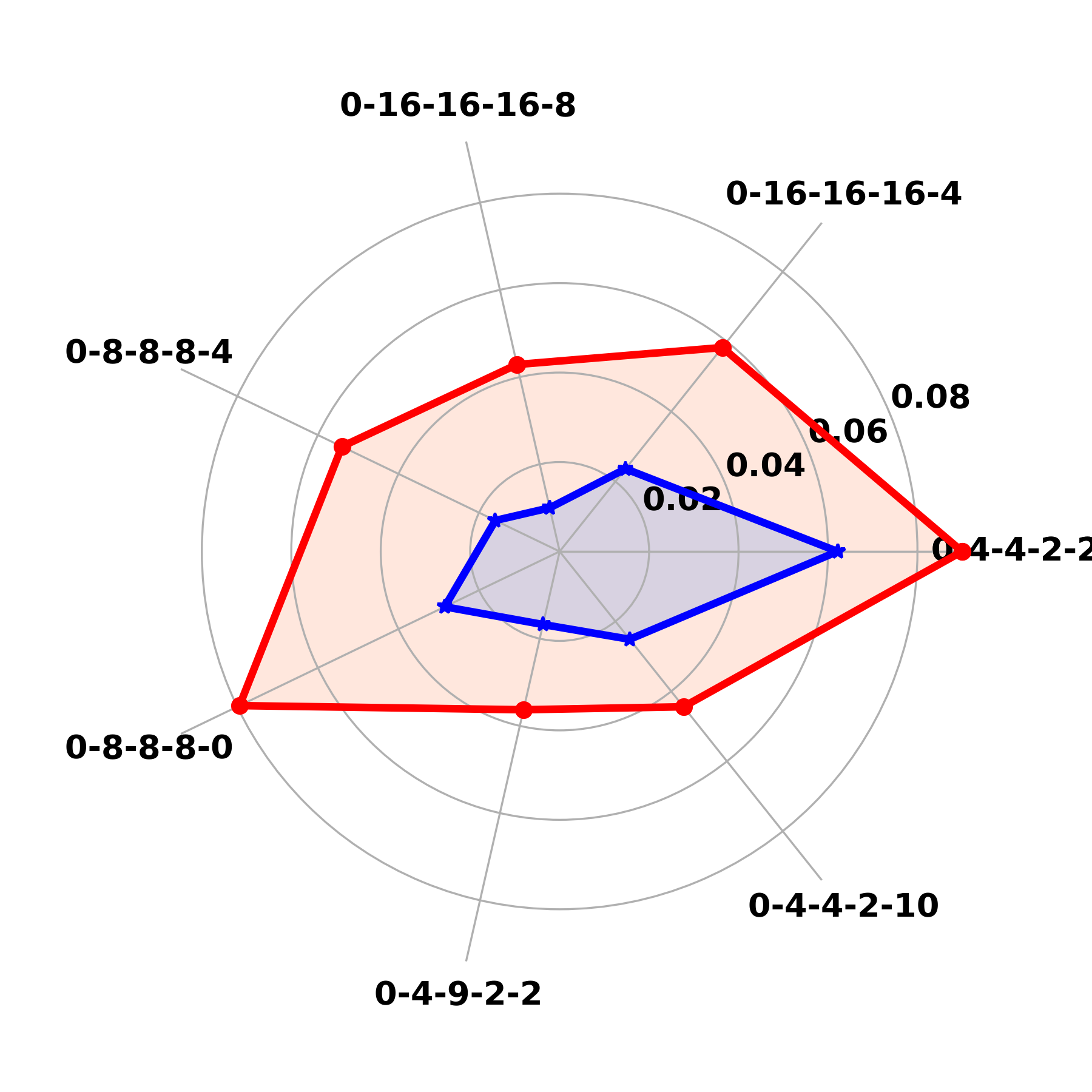
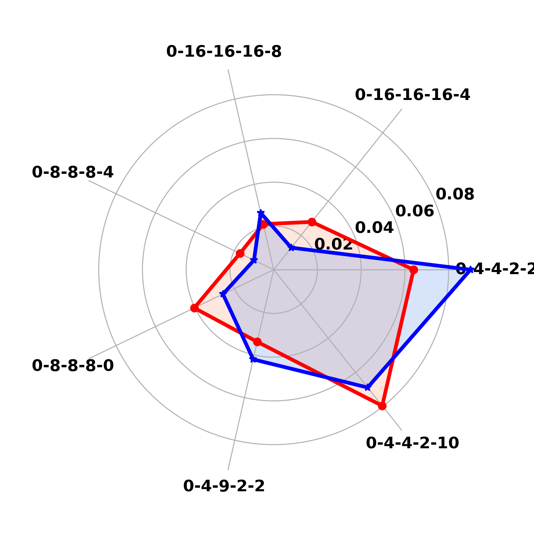
5.3.2. Disentanglement Visualization
To check if decompose different kinds of underlying factors from pre-treatment variables successfully, similar to Hassanpour and Greiner (2019), we use the first (second) slice to denote the weight matrix that connects the variables in X belonging (not belonging) to the actual variables. The polygons’ radii in Figure 5 quantify the average weights of the first slice (in red) and the second slice (in blue). We plot the radar charts to visualize the contribution of actual variables to the representations of each factor on and another typical causal disentangled learning work DRCFR.
As shown in each sub-figure in Figure 5, each vertex on the polygon represents the results of a synthetic dataset ----. Compared with DRCFR, our method realizes much better identification performance of all three underlying factors in all datasets, indicating that our approach can achieve successful disentanglement performance.

5.3.3. Difficulty of mutual information estimation
To quantify the difficulty of high-dimensional mutual information estimation, we substitute our core disentanglement module with one of the state-of-the-art mutual information estimators, CLUB (Cheng et al., 2020), which has been widely adopted in previous causal disentangled learning methods (Wu et al., 2020; Yuan et al., 2022; Cheng et al., 2022b), aiming to directly minimize the mutual information between , , and . The related experimental results ( in Table 3) show that the performance of our method gets impeded dramatically, indicating the importance of bypassing the complex mutual information estimation.
5.3.4. Ablation Study
We perform the ablation experiments to examine the contributions of each component in total loss function on final inference performance. The results are shown in Table 4. We conduct following steps for the ablation study analysis.
-
•
Firstly, we only preserve representation networks and deep outcome prediction networks. The objective loss is reduced to factual loss plus regularization loss.
-
•
Secondly, we add the deep treatment prediction networks into the model on the basis of the first model, while the objective loss becomes .
-
•
Then, the adjustable variables decomposition module is integrated into the second model, thus the objective loss is .
-
•
Finally, we introduce our shallow treatment and outcome prediction networks into the third model, the objective loss of which is presented in Eq (11) in the main paper and named as .
We have the following observations from the experimental results in Table 4:
-
•
The model with loss function performs the worst for all data settings on all datasets, demonstrating the significance of treatment prediction for counterfactual prediction in the presence of unobserved confounders.
-
•
If we only decompose adjustable variables from observed features , as the results under the loss shows, the model indeed does not get much improvement on the inference performance compared with the results under the loss . This may be due to the fact that only decomposing A cannot eliminate the confounding bias caused by the unmeasured confounders and underlying confounders existing in observed features . In addition, it indicates the necessity of the decomposition of and for counterfactual prediction.
-
•
When added shallow prediction networks of treatment and outcome during training, as the results of model show, our achieves the best performance with the improvement of more than on Synthetic datasets and over on Twins datasets on the basis of the model under the loss , which demonstrates the decomposition of and indeed advances the counterfactual inference.
5.3.5. Hyper-Parameters Analysis
With the multi-term total loss function shown in Eq (11), we study the impact of each item on the counterfactual prediction on Syn-0-4-4-2-2 dataset. As can be seen from Figure 6, the performance of is mostly affected by the changing in . In addition, although the performance fluctuates with the change of and , performs better than almost all baselines. These two facts demonstrate that the improvement of inference performance is greatly contributed by the decomposition of and . Besides, from Figure 6, we find that the performance of the method is affected by changing as well, indicating the necessity of limiting the complexity of the model.
5.3.6. Scalability Analysis
To demonstrate the scalability of our algorithm, we conduct experiments on Syn-0-4-4-2-2 with different sample sizes with our method and DRCFR (Hassanpour and Greiner, 2019). Figure 7 shows the results of the related experimental results. It can be seen from the results that the performance of remains stable and efficient with the variation of sample size in the dataset, which demonstrates the scalability of our algorithm.
6. Conclusion and Limitations
To resolve the challenge of decomposing mutually independent underlying factors in causal disentangled learning study, we provide a theoretically guaranteed solution to minimizing the mutual information between representations of diverse underlying factors instead of relying on explicit estimation. On this basis, we design a hierarchical self-distilled disentanglement framework to advance counterfactual prediction by eliminating the confounding bias caused by the observed and unobserved confounders simultaneously. Extensive experimental results on synthetic and real-world datasets validate the effectiveness, generalizability, scalability of our proposed theory and framework in both binary and continuous data settings.
Limitations: Due to the lack of real-world counterfactual datasets, is only evaluated on limited tasks. It would be interesting to extend our method into other research areas, such as transfer learning (Rojas-Carulla et al., 2015), domain adaptation (Magliacane et al., 2017), counterfactual fairness (Kim et al., 2020), for robust feature extraction. We will leave future work for the generalization of our method to these fields.
References
- (1)
- Alaa and van der Schaar (2017) Ahmed M Alaa and Mihaela van der Schaar. 2017. Bayesian inference of individualized treatment effects using multi-task gaussian processes. Advances in Neural Information Processing Systems 30 (2017).
- Almond et al. (2005) Douglas Almond, Kenneth Y Chay, and David S Lee. 2005. The costs of low birth weight. The Quarterly Journal of Economics 120, 3 (2005), 1031–1083.
- Angrist and Imbens (1994) Joshua David Angrist and Guido Imbens. 1994. Identification and Estimation of Local Average Treatment Effects. NBER Working Paper Series (1994).
- Angrist et al. (1996) Joshua D Angrist, Guido W Imbens, and Donald B Rubin. 1996. Identification of causal effects using instrumental variables. Journal of the American statistical Association 91, 434 (1996), 444–455.
- Belghazi et al. (2018) Mohamed Ishmael Belghazi, Aristide Baratin, Sai Rajeshwar, Sherjil Ozair, Yoshua Bengio, Aaron Courville, and Devon Hjelm. 2018. Mutual information neural estimation. In International conference on machine learning. PMLR, 531–540.
- Chen et al. (2016) Xi Chen, Yan Duan, Rein Houthooft, John Schulman, Ilya Sutskever, and P. Abbeel. 2016. InfoGAN: Interpretable Representation Learning by Information Maximizing Generative Adversarial Nets. In NIPS.
- Cheng et al. (2022a) Lu Cheng, Ruocheng Guo, Kasim Candan, and Huan Liu. 2022a. Effects of Multi-Aspect Online Reviews with Unobserved Confounders: Estimation and Implication. In Proceedings of the International AAAI Conference on Web and Social Media, Vol. 16. 67–78.
- Cheng et al. (2022b) Mingyuan Cheng, Xinru Liao, Quan Liu, Bin Ma, Jian Xu, and Bo Zheng. 2022b. Learning disentangled representations for counterfactual regression via mutual information minimization. In Proceedings of the 45th International ACM SIGIR Conference on Research and Development in Information Retrieval. 1802–1806.
- Cheng et al. (2020) Pengyu Cheng, Weituo Hao, Shuyang Dai, Jiachang Liu, Zhe Gan, and Lawrence Carin. 2020. CLUB: A Contrastive Log-ratio Upper Bound of Mutual Information. In International Conference on Machine Learning.
- Chernozhukov et al. (2013) Victor Chernozhukov, Iván Fernández-Val, and Blaise Melly. 2013. Inference on counterfactual distributions. Econometrica 81, 6 (2013), 2205–2268.
- Chipman et al. (2010) Hugh A Chipman, Edward I George, and Robert E McCulloch. 2010. BART: Bayesian additive regression trees. The Annals of Applied Statistics 4, 1 (2010), 266–298.
- Glass et al. (2013) Thomas A Glass, Steven N Goodman, Miguel A Hernán, and Jonathan M Samet. 2013. Causal inference in public health. Annual review of public health 34 (2013), 61.
- Goodfellow et al. (2014) Ian J. Goodfellow, Jean Pouget-Abadie, Mehdi Mirza, Bing Xu, David Warde-Farley, Sherjil Ozair, Aaron C. Courville, and Yoshua Bengio. 2014. Generative Adversarial Nets. In NIPS.
- Hartford et al. (2017) Jason Hartford, Greg Lewis, Kevin Leyton-Brown, and Matt Taddy. 2017. Deep IV: A flexible approach for counterfactual prediction. In International Conference on Machine Learning. PMLR, 1414–1423.
- Hassanpour and Greiner (2019) Negar Hassanpour and Russell Greiner. 2019. Learning disentangled representations for counterfactual regression. In International Conference on Learning Representations.
- Higgins et al. (2017) Irina Higgins, Loic Matthey, Arka Pal, Christopher Burgess, Xavier Glorot, Matthew Botvinick, Shakir Mohamed, and Alexander Lerchner. 2017. beta-VAE: Learning Basic Visual Concepts with a Constrained Variational Framework. In International Conference on Learning Representations. https://openreview.net/forum?id=Sy2fzU9gl
- Hoxby (2000) Caroline M Hoxby. 2000. Does competition among public schools benefit students and taxpayers? American Economic Review 90, 5 (2000), 1209–1238.
- Imbens (2004) Guido W Imbens. 2004. Nonparametric estimation of average treatment effects under exogeneity: A review. Review of Economics and statistics 86, 1 (2004), 4–29.
- Kim and Mnih (2018) Hyunjik Kim and Andriy Mnih. 2018. Disentangling by Factorising. In International Conference on Machine Learning.
- Kim et al. (2020) Hyemi Kim, Seungjae Shin, Joonho Jang, Kyungwoo Song, Weonyoung Joo, Wanmo Kang, and Il-Chul Moon. 2020. Counterfactual Fairness with Disentangled Causal Effect Variational Autoencoder. ArXiv abs/2011.11878 (2020).
- Kingma and Welling (2013) Diederik P. Kingma and Max Welling. 2013. Auto-Encoding Variational Bayes. CoRR abs/1312.6114 (2013).
- Li and Yao (2022) Xinshu Li and Lina Yao. 2022. Contrastive Individual Treatment Effects Estimation. In 2022 IEEE International Conference on Data Mining (ICDM). 1053–1058. https://doi.org/10.1109/ICDM54844.2022.00130
- Li and Yao (2024) Xinshu Li and Lina Yao. 2024. Distribution-Conditioned Adversarial Variational Autoencoder for Valid Instrumental Variable Generation. In Proceedings of the AAAI Conference on Artificial Intelligence, Vol. 38. 13664–13672.
- Lin et al. (2019) Adi Lin, Jie Lu, Junyu Xuan, Fujin Zhu, and Guangquan Zhang. 2019. One-stage deep instrumental variable method for causal inference from observational data. In 2019 IEEE International Conference on Data Mining (ICDM). IEEE, 419–428.
- Louizos et al. (2017) Christos Louizos, Uri Shalit, Joris M. Mooij, David A. Sontag, Richard S. Zemel, and Max Welling. 2017. Causal Effect Inference with Deep Latent-Variable Models. In NIPS.
- Magliacane et al. (2017) Sara Magliacane, Thijs van Ommen, Tom Claassen, Stephan Bongers, Philip Versteeg, and Joris M. Mooij. 2017. Domain Adaptation by Using Causal Inference to Predict Invariant Conditional Distributions. In Neural Information Processing Systems.
- Muandet et al. (2020) Krikamol Muandet, Arash Mehrjou, Si Kai Lee, and Anant Raj. 2020. Dual instrumental variable regression. Advances in Neural Information Processing Systems 33 (2020), 2710–2721.
- Pearl et al. (2000) Judea Pearl et al. 2000. Models, reasoning and inference. Cambridge, UK: CambridgeUniversityPress 19 (2000), 2.
- Poole et al. (2019) Ben Poole, Sherjil Ozair, Aaron Van Den Oord, Alex Alemi, and George Tucker. 2019. On variational bounds of mutual information. In International Conference on Machine Learning. PMLR, 5171–5180.
- Puli and Ranganath (2020) Aahlad Puli and Rajesh Ranganath. 2020. General Control Functions for Causal Effect Estimation from IVs. Advances in neural information processing systems 33 (2020), 8440–8451.
- Rojas-Carulla et al. (2015) Mateo Rojas-Carulla, Bernhard Schölkopf, Richard E. Turner, and J. Peters. 2015. Invariant Models for Causal Transfer Learning. J. Mach. Learn. Res. 19 (2015), 36:1–36:34.
- Rosenbaum and Rubin (1983) Paul R Rosenbaum and Donald B Rubin. 1983. The central role of the propensity score in observational studies for causal effects. Biometrika 70, 1 (1983), 41–55.
- Shalit et al. (2017) Uri Shalit, Fredrik D Johansson, and David Sontag. 2017. Estimating individual treatment effect: generalization bounds and algorithms. In International Conference on Machine Learning. PMLR, 3076–3085.
- Singh et al. (2019) Rahul Singh, Maneesh Sahani, and Arthur Gretton. 2019. Kernel instrumental variable regression. Advances in Neural Information Processing Systems 32 (2019).
- Veitch et al. (2020) Victor Veitch, Dhanya Sridhar, and David Blei. 2020. Adapting text embeddings for causal inference. In Conference on Uncertainty in Artificial Intelligence. PMLR, 919–928.
- Veitch et al. (2019) Victor Veitch, Yixin Wang, and David Blei. 2019. Using embeddings to correct for unobserved confounding in networks. Advances in Neural Information Processing Systems 32 (2019).
- Wang and Blei (2019) Yixin Wang and David M Blei. 2019. The blessings of multiple causes. J. Amer. Statist. Assoc. 114, 528 (2019), 1574–1596.
- Wooldridge (2015) Jeffrey M. Wooldridge. 2015. Control Function Methods in Applied Econometrics. Journal of Human Resources 50, 2 (2015), 420–445. https://doi.org/10.3368/jhr.50.2.420 arXiv:https://jhr.uwpress.org/content/50/2/420.full.pdf
- Wu et al. (2022a) Anpeng Wu, Kun Kuang, Bo Li, and Fei Wu. 2022a. Instrumental variable regression with confounder balancing. In International Conference on Machine Learning. PMLR, 24056–24075.
- Wu et al. (2022b) Anpeng Wu, Kun Kuang, Ruoxuan Xiong, Minqing Zhu, Yuxuan Liu, Bo Li, Furui Liu, Zhihua Wang, and Fei Wu. 2022b. Treatment Effect Estimation with Unmeasured Confounders in Data Fusion. ArXiv abs/2208.10912 (2022).
- Wu et al. (2020) Anpeng Wu, Kun Kuang, Junkun Yuan, Bo Li, Runze Wu, Qiang Zhu, Yueting Zhuang, and Fei Wu. 2020. Learning decomposed representation for counterfactual inference. arXiv preprint arXiv:2006.07040 (2020).
- Wu and Fukumizu (2022) Pengzhou Abel Wu and Kenji Fukumizu. 2022. $\beta$-Intact-VAE: Identifying and Estimating Causal Effects under Limited Overlap. In International Conference on Learning Representations. https://openreview.net/forum?id=q7n2RngwOM
- Xu et al. (2020) Liyuan Xu, Yutian Chen, Siddarth Srinivasan, Nando de Freitas, Arnaud Doucet, and Arthur Gretton. 2020. Learning deep features in instrumental variable regression. arXiv preprint arXiv:2010.07154 (2020).
- Yao et al. (2018) Liuyi Yao, Sheng Li, Yaliang Li, Mengdi Huai, Jing Gao, and Aidong Zhang. 2018. Representation learning for treatment effect estimation from observational data. Advances in Neural Information Processing Systems 31 (2018).
- Yuan et al. (2022) Junkun Yuan, Anpeng Wu, Kun Kuang, Bo Li, Runze Wu, Fei Wu, and Lanfen Lin. 2022. Auto IV: Counterfactual Prediction via Automatic Instrumental Variable Decomposition. ACM Transactions on Knowledge Discovery from Data (TKDD) 16, 4 (2022), 1–20.
- Zhang et al. (2019) Linying Zhang, Yixin Wang, Anna Ostropolets, Jami J Mulgrave, David M Blei, and George Hripcsak. 2019. The medical deconfounder: assessing treatment effects with electronic health records. In Machine Learning for Healthcare Conference. PMLR, 490–512.
- Zhang et al. (2021) Weijia Zhang, Lin Liu, and Jiuyong Li. 2021. Treatment effect estimation with disentangled latent factors. In Proceedings of the AAAI Conference on Artificial Intelligence, Vol. 35. 10923–10930.
- Zhou et al. (2023) Guanglin Zhou, Shaoan Xie, Guangyuan Hao, Shiming Chen, Biwei Huang, Xiwei Xu, Chen Wang, Liming Zhu, Lina Yao, and Kun Zhang. 2023. Emerging synergies in causality and deep generative models: A survey. arXiv preprint arXiv:2301.12351 (2023).
- Zhou et al. (2022) Guanglin Zhou, Lina Yao, Xiwei Xu, Chen Wang, and Liming Zhu. 2022. Cycle-Balanced Representation Learning For Counterfactual Inference. In Proceedings of the 2022 SIAM International Conference on Data Mining (SDM). SIAM, 442–450.
- Zou et al. (2020) Yang Zou, Xiaodong Yang, Zhiding Yu, B. V. K. Vijaya Kumar, and Jan Kautz. 2020. Joint Disentangling and Adaptation for Cross-Domain Person Re-Identification. ArXiv abs/2007.10315 (2020).
Appendix A Appendix
A.1. Theoretical Proof
A.1.1. Proof of Theorem 4.1
Consider and as the representations of and produced by the representation networks, and let Y be the label of the outcome. We have,
Proof.
Based on the definition of mutual information (Belghazi et al., 2018):
| (15) |
where denotes Shannon entropy, and is the conditional entropy of given . Similarly,
| (16) |
where denotes the conditional mutual information between and given ; and is the the conditional entropy of given , and , respectively.
A.1.2. Proof of Corollary 4.2
One of sufficient conditions of minimizing is:
where , represent the predicted distributions, represents the real distribution, and denotes the KL-divergence.
Proof.
Based on the definition of conditional entropy, for any continuous variables , and , we have:
| (18) |
We further inspect in Eq (18) and have:
| (19) |
By factorizing the double integrals in Eq (19) into another two components, we show the following:
| (20) |
Conduct similar factorization for and in Eq (18), we have:
| (21) |
| (22) |
Integrate , and over :
| (23) |
| (24) |
| (25) |
where denotes KL-divergence. Integrate and over and , respectively, we have:
| (26) |
| (27) |
Integrate over , we have:
| (28) |
We further factorize Eq (28) into another two components:
| (29) |
In the view of above, we have the following:
| (30) |
Based on the non-negativity of KL-divergence, Eq (30) is upper bounded by:
| (31) |
Equivalently, we have the upper bound as:
| (32) |
where , denote the parameters of the representation networks of and , respectively. Therefore, the objective of separating and from can be formalized as:
| (33) |
where , and denote the predicted distributions of from the representations , and real distribution of , respectively.
Clearly, the first term in Eq (33) is equivalent to minimize the discrepancy between the predicted distributions of from the representations , . Notice the second term in Eq (33) can be implicitly reduced by minimizing . Thus, we have:
Corol.4.2 holds. ∎
A.2. Reproducibility
A.2.1. Loss Functions for Continuous Scenario
The loss function for disentangling A is defined as following:
| (35) |
where in represents the predicted values for while in it denotes the distribution of the variable. Same below.
We assume that the continuous variable follows a normal distribution, therefore the KL divergence can be calculated with:
| (36) |
where .
To reduce the confounding bias led by observed confounders, we define the following loss function:
| (37) |
where denotes the representation of after re-balance network.
Therefore, the total loss function of for the continuous scenario can be devised as:
| (38) |
A.2.2. Hardware
In this work, we perform all experiments on a cluster with two 12-core Intel Xeon E5-2697 v2 CPUs and a total 768 GiB Memory RAM.