Can market volumes reveal traders’ rationality and a new risk premium?

Abstract

An empirical analysis, suggested by optimal Merton dynamics, reveals some unexpected features of asset volumes. These features are connected to traders’ belief and risk aversion. This paper proposes a trading strategy model in the optimal Merton framework that is representative of the collective behavior of heterogeneous rational traders. This model allows for the estimation of the average risk aversion of traders acting on a specific risky asset, while revealing the existence of a price of risk closely related to market price of risk and volume rate. The empirical analysis, conducted on real data, confirms the validity of the proposed model.

Keywords: Merton problem, stochastic control problems, market frictions

1 Introduction

The Merton portfolio problem with HARA utility functions provides the optimal solution, which suggests that the number of shares invested in a risky asset follows a geometric Brownian motion. Interestingly, this dynamics is characterized by a constant ratio between the drift term and the diffusion term over time. This ratio is independent of the investor’s risk aversion and depends solely on the risk-free rate, price rate, and volatility (see Mariani et al. 2019 [16]). Moreover, the dynamics of volume and price are characterized by the same Wiener process.

The paper makes a threefold contribution.

Firstly, we examine whether the dynamics of asset volume exhibit features consistent with those outlined by the Merton model. To accomplish this, we assume that the volume is a diffusion process and we calculate the drift-to-diffusion ratio of volume process for multiple assets. Our estimations indicate that this ratio remains relatively stable over extended time periods, with minor fluctuations observed across various asset classes. However, notably, the estimated ratios diverge significantly from those prescribed by the Merton optimal portfolio, except for market indices such as the S& P 500 and Nasdaq. Furthermore, empirical analysis reveals that asset and volume dynamics do not share the same Wiener process. This finding is further supported by the results of Carmona and Webster (2013) [5] and suggests the presence of market inefficiencies.

Secondly, assuming that asset volume serves as a proxy for the number of shares invested by a representative trader in the risky asset, we derive the dynamics of the trader’s wealth invested in aforementioned asset. The drift and diffusion of this wealth dynamics are straightforward functions of both the asset price’s drift and diffusion, as well as the volume trading rate.

Furthermore, imposing no arbitrage possibility, that is imposing that both the discounted wealth and price reduce to martingales, we show that the the drift-to-volatility ratio of volume process must coincide with that prescribed by Merton optimal consumption model. However, the empirical analysis provides evidence that the observed ratio does not coincide with the theoretical one, revealing the presence of inefficiencies on the market generated by the trading activity. This evidence is reinterpreted in a frictionless Merton framework in terms of an impacted asset price and of a new price of risk.

This new price of risk can be estimated from both price and volume data and, surprisingly, it closely aligns with what is outlined by Prospect Theory as illustrated in Kahneman and Tversky (1979) [11] and Kahneman and Tversky (1991) [12] (refer to Section 3). We refer to this as the trading price of risk because its measures the extra return that investors demand to bear risk in presence of trading. Naturally, the trading price of risk reduces to the market price of risk in absence of trading, interestingly, in this case, the drift-to-diffusion ratio coincides with the Merton one.

Finally, the most intriguing contribution is the derivation of the price impact and the average risk aversion of the traders acting on that specific asset. The impacted asset price is determined by reinterpreting the observed wealth invested in the risky asset as the wealth invested in an ideal risky asset (the impacted price) by a representative trader.

We show that the (observable) trading strategy of the representative trader arises as the limit of the optimal trading strategies employed by traders investing in the risky asset and a risk-free asset, as the number of traders tends toward infinity. The parameters, characterizing the strategy dynamics at micro-level, are drawn by independent and identically distributions whose mean values we prove to be the parameters of the strategy dynamics at the macro-level.

Summing up, from a practical standpoint, our paper shows the deviation of the observed drift-to-volatility ratio of volume from the theoretical ratio and justifies this deviation as the effect of market inefficiencies. This deviation implies a change in the market price of risk which, in turn, implies a change in the risk-neutral world with a price impact. Notably, from the drift-to-volatility ratio of trading volume and the price volatility we can estimate the experienced trading price of risk.

In order to assess the validity of our model, we analyze the data relative to the daily trading volume and the stock quotes from the exchanged on NYSE (New York Stock Exchange) for three companies are used: PFE (Pfizer Inc.), a research-based biopharmaceutical company, VZ (Verizon Communications Inc.), a communication service company and Coca Cola. Moreover, we use the three months treasury bill yield as a proxy for the risk-free interest rate.

Despite the geometric brownian motion is a questionable dynamics for asset prices and volumes, we provide empirical evidence that the volume drift-to-volatility ratio is constant over time but deviates from the Merton one. Specifically, we propose two empirical study. The first one aims to show that the observed ratio is constant over time and the experienced price of risk (the trading price of risk) is around 2.5-3 if the analyzed assets have been traded in the financial market for long time. The second analysis considers a very long trading period and aims to show that the trading price of risk is higher at the very beginning of asset life. We observe that the trading price of risk is a piecewise constant function of time. The higher value is approximately 5.5-6 in the oldest dates while converging to 2.5-3 at the most recent dates. Our findings regarding the price of risk is in line with the Prospect Theory as illustrated in Kahneman and Tversky (1991) [12].

Our work is related to different strands of scientific literature.

Firstly, the literature which try to generalize frictionless Merton portfolio optimization to include market friction. In [6] Chebbi and Soner (2013) propose a discrete time Merton model with frictions in an infinite horizon for multiple investors introducing a penalty in the wealth dynamics due to the trading. In [7] Chebbi and Ounaies (2023) extend the model introduced in [6] to consider multiple investors and derive the optimal trading strategy using an approach based on the general equilibrium theory of Le Van and Dana (2003) [15]. Mariani et al. (2019) in [16] model the presence of frictions including a penalty in the utility function of Merton problem in continuous time. Assuming the penalty to be a specific function of trading rate, the problem is solved explicitly using as control the trading rate itself. Interestingly, the solution is re-interpreted as the optimal trading strategy in a frictionless Merton market for a shadow price.

Secondly, the literature regarding the impact of trading on asset prices. Models for price impacts have been widely studied, for a survey of them refer to Bouchaud (2017) [3]. In [10] He and Mamaysky (2005) address the problem of liquidating a large block of a risky asset shares in presence of price impact and transaction costs. In [8] Chen (2019) empirically examines whether trade-size clustering, which measures trading irregularity, has an impact on price formation. In [9] Gatheral (2010) investigates a relationship between the shape of the market impact function and the decay of market impact.

Lastly, the literature regarding the Prospect Theory of Kahneman and Tversky (1991) [12]. The central assumption of this theory is that losses and disadvantages have greater impact on preferences than gains and advantages. Implications of loss aversion for economic behavior are considered. Kahneman and Tversky propose an empirical experiments suggesting that a loss aversion coefficient of about 2-2.5 may explain both risky and riskless choices involving monetary outcomes and consumption goods. Surprisingly the price of risk experienced from the trading volume shows the same value for assets with a long life in the financial market.

The paper is structured as follows: Section 2 presents the empirical finding and, starting from the observed volume dynamics, introduces a model for the fraction of wealth invested in the risky asset. Section 3 proposes an interpretation for the model introduced in Section 2 based on a representative agent model describing the aggregate behavior of rational heterogeneous traders. Section 4 proposes an empirical analysis where the experienced risk premium and the market risk aversion are estimated.

2 Empirical finding and implications

We start from empirical findings obtained by looking the time series of the volumes and prices of different assets. For simplicity we assume that the asset price process is a geometric Brownian motion:

$$dS_{t}=S_{t}\left(\mu_{t}dt+\sigma_{t}dZ_{t}\right),\quad t\in[0,T],$$ (1)

where $\mu_{t}$ and $\sigma_{t}$ are the drift and volatility of asset price, $Z_{t}$, $t>0$, is a Brownian motion while $dZ_{t}$ is its differential. We estimate the volatility of the price process, $\sigma_{t}$ using a year of consecutive price daily observations backward from $t$ to $t-252$.

Further, we empirically observe:

1. The volume process, $n_{t}$, $t>0$, is a diffusion as, already stated in Carmona and Webster (2013) [5]:

   $$dn_{t}=n_{t}(\mu^{v}_{t}dt+\sigma^{v}_{t}dQ_{t}),\quad t\in[0,T],$$ (2)

   where $Q_{t}$, $t>0$, is a Brownian motion while $dQ_{t}$ is its differential;

2. the ratio, $\mu_{t}^{v}/\sigma^{v}_{t}$ (i.e., drift-to-diffusion) of the volume process is a piecewise constant function of time.

3. The ratio $\mu_{t}^{v}/\sigma^{v}_{t}$ multiplied by $\sigma_{t}$ (i.e., the price volatility) is a piecewise constant function with respect to time, so implying the existence of a relationship between volume volatility and asset volatility; therefore, without loss of generality, we can rewrite the drift and the diffusion terms as follows: $\mu_{t}^{v}=\_t\psi_{t}$, $\sigma^{v}_{t}=\eta_{t}\sigma_{t}$. The dynamics of the volume looks like:

   $$dn_{t}=n_{t}\eta_{t}(\psi_{t}\,dt+\sigma_{t}\,dQ_{t}),\quad t\in[0,T].$$ (3)

4. The Brownian motions which define the asset and volume processes are correlated but with a weakly correlation. That is, we have

   $$E(dZ_{t},dQ_{t})=\rho dt,$$ (4)

   where $\rho\approx 0.$

The main consequence of dynamics (1), (2) and (4) is the dynamics for the wealth invested in the risky asset, $\pi_{t}=n_{t}S_{t},$ is:

$$d\pi_{t}=\pi_{t}\left[\left(\mu_{t}+(\psi_{t}+\rho_{t}\sigma_{t}^{2})\eta_{t}\right)dt+\sigma_{t}(dZ_{t}+\eta_{t}dQ_{t})\right],\quad t\in[0,T].$$ (5)

Note that the wealth invested in the risk asset, i.e., $\pi_{t}$, given in Eq. (5) depends on two noises, $Z_{t},$ related to the fundamentals of the asset $S_{t},$ while $Q_{t}$ is related to the agents’ trading and the agents’ beliefs.

In this market, no arbitrage principle should hold, thus, there exists a change of measure that allows the discounted processes $e^{-rt}S_{t}$, $e^{-rt}\pi_{t}$ to be martingales. Here $r$ is the risk free interest rate. This change that guarantees the no-arbitrage principle in pricing is given by

$$dZ_{t} = d\widetilde{Z}_{t}-\frac{(\mu-r)}{\sigma_{t}}dt,$$ (6)

$$dQ_{t} = d\widetilde{Q}_{t}-\frac{(\psi_{t}+\rho\sigma_{t}^{2})\eta_{t}}{\eta_{t}\sigma_{t}}dt\,.$$ (7)

The change of measure reveals the presence of two risks. The market price of risk ${\varphi_{p}}=\frac{(\mu-r)}{\sigma_{t}}$ measures the extra gain in terms of price volatility units that a trader requires to take on the price risk compared to investing in a guaranteed income security. The volume price of risk:

$${\varphi_{v}}=\frac{\eta_{t}(\psi_{t}+\sigma_{t}^{2}\rho)}{\eta_{t}\sigma_{t}}=\frac{(\psi_{t}+\sigma_{t}^{2}\rho)}{\sigma_{t}}$$ (8)

measures the extra gain in terms of volume volatility units that a trader requires to take on the strategy risk $\pi_{t}$ compared to investing in a strategy consisting only of guaranteed income security. which is well-know and interpretable as the compensation for each unit of volatility risk.

We can rewrite $\pi_{t}$ using a new Brownian motion which is the linear combination of the previous two as follows:

$$d\pi_{t}=\pi_{t}\left[\left(\mu_{t}+(\psi_{t}+\rho_{t}\sigma_{t}^{2})\eta_{t}\right)dt+\sigma_{t}\sqrt{1+\eta_{t}^{2}+2\rho_{t}\eta_{t}}dW_{t}\right],\quad t\in[0,T].$$ (9)

Remark Note that in a complete market, if the no arbitrage principle hold, thus, there exists only one change of measure that allows the discounted processes $e^{-rt}\pi_{t},$ $e^{-rt}S_{t}$ to be a martingale. This is possible if the Brownian motions $Z_{t},$ $Q_{t}$ coincide, or, equivalently, $\rho_{t}=1$ in Eq. (4) and the volume price of risk coincides with the market price of risk, i.e.:

$$\frac{\psi_{t}+\sigma_{t}^{2}}{\sigma_{t}}=\frac{\mu_{t}-r}{\sigma_{t}}.$$ (10)

It is evident that Eq. (10) holds true when the drift-to-volatility ratio of volume equals the Merton value, i.e., $\psi_{t}/\sigma_{t}=(\mu_{t}-r)/\sigma_{t}-\sigma_{t}$ (refer to Mariani et al. 2019 formula (44)).

However, the empirical analysis, carried out in Section 4, shows that the value of observed ratio does not coincide with the theoretical ratio prescribed by Merton. This suggests the presence of market inefficiencies. Specifically, we expect that, the greater the distance between the observed ratio and the theoretical ratio, the greater the market inefficiencies.

If the ratio prescribed in Eq. (10) is not true to preserve the no arbitrage principle, it should be allowed for an impacted price and explain why the trading strategy is rational.

3 Optimal consumption and average risk aversion

In this section we interpret the empirical findings of Section 2 in terms of optimal consumption in the frictionless Merton framework for an impacted asset price to address two delicate issues: a) is the risk aversion parameter measurable from observed data? b) can the volumes reveal the rationality of traders?

We hypothesize that, in the presence of market inefficiency, trading affects the dynamics of the wealth invested in the risky asset price. This renders Merton’s frictionless market unrealistic, especially the assumption of a single noise driving uncertainty. Market findings suggest that agents face two risks: one due to asset performance driven by asset Brownian motion, and a second due to information circulating in the market, which can modify agents’ beliefs (see, for example, Borgonovo et al. (2018) [1] and Borgonovo et al. (2019) [2]).

The crucial assumption is that the financial market acts by implementing its optimal strategy, $\pi_{t}$ in Eq. (9), i.e., the dynamics of the wealth invested in the risky asset is the optimal one. Therefore, we look for the “ideal” price which allows us to get the observed wealth invested in the risky asset, $\pi_{t}$, as the optimal dynamics in the Merton frictionless framework. The ideal price is the impacted price announced in the Introduction. So doing, we obtain the market risk aversion as a function of the observed parameters of price and volume dynamics, along with the relationship between the drift and the volatility of the impacted price with the parameters of the price and volume dynamics.

In order to recover the dynamics of the impacted price and to estimate the market risk aversion we propose a representative agent model for describing the aggregate behavior of rational heterogeneous traders. Specifically, we model the traders as individuals with different beliefs about the drift and volatility of the risky asset price and with different risk aversions. Under some suitable assumptions about the parameters of the risky asset price dynamics and the risk aversions, we derive the aggregate trading dynamics as limit of the trading strategies of traders, as the number of traders goes to infinity.

Specifically, in our model, each trader acts rationally solving his Merton problem. As a consequence, the optimal trading strategies, derived as solution of the Merton problem, associated with different traders are different. Assuming traders be independent and share the same distribution of the risk aversion and the same distribution of the risk-adjusted price of risk, we show that, when the number of traders is large enough, the individual strategies of traders are independent copies of the same process under different risk aversions and risk-adjusted price of risk. We call this process generator process. This allows to derive the dynamics of the generator process as the limit dynamics of the individual optimal trading strategies when the number of traders goes to infinity. This dynamics is given by a diffusion process with drift and volatility expressed in terms of the market risk aversion and of the mean and of the variance of risk-adjusted price of risk.

Finally, the aggregate trading strategy is interpreted as the strategy of an “ideal” average trader with risk aversion given by the market risk aversion, which operates in a frictionless Merton market on an “ideal” risky asset, the impacted risky asset, whose price drift and volatility depends on the mean and on the variance of risk-adjusted price of risk. This ideal trader is the fictitious representative trader, that represents the multitude of traders at macroscopic level when the number of traders is large enough.

In what follows we propose a mathematical formalization for our model.

We have $N$ traders, each of them has a different belief about the risky asset price drift and volatility and a different risk aversion.

Denoting by $S_{i,t},$ $t\in[0,T],$ the price associated with the $i-$th trader, for $i=1,2,\ldots,N,$ we assume that $S_{i,t}$ are Îto processes, evolving according to the Stochastic Differential Equation (SDE) system

$$\frac{dS_{i,t}}{S_{i,t}}=\mu_{i,t}dt+\sigma_{i,t}dW_{i,t},\quad t\in[0,T],$$ (11)

where $W_{i,t},$ $t\in[0,T],$ $i=1,2,\ldots,N,$ are $N$ independent standard Brownian motions.

In Eq. (11) the quantities $\mu_{i,t}$ and $\sigma_{i,t},$ are, respectively, the return and the volatility of price perceived by the $i-$th trader, $i=1,2,\ldots,N.$

We denote by $B_{t}$ the price of the risk-free asset at time $t,$ $t\in[0,T],$ which satisfies the following deterministic differential equation:

$$dB_{t}=rB_{t}dt,t\in[0,T],$$ (12)

where $r>0$ is a risk-free interest rate, and $B(0)=1.$ In other words, all traders share the same view on the risk free return.

Given $n^{B}_{i,t}$ and $n_{i,t}$ the number of shares invested, respectively, in the risk-free asset and in the risky asset with price $S_{i,t}$ at time $t,$ $t\in[0,T],$ the total portfolio wealth of trader $i,$ $x_{i,t},$ $t\in[0,T],$ reads:

$$x_{i,t}=n_{i,t}S_{i,t}+n^{B}_{i,t}B_{t},\quad t\in[0,T],\,i=1,2,\ldots,N.$$ (13)

Moreover, assuming the self-financing condition, the dynamics of $x_{i,t}$ is given by

$$dx_{i,t}=[x_{i,t}r+n_{i,t}S_{i,t}(\mu_{i,t}-r)]dt+n_{i,t}S_{i,t}\sigma_{i,t}dW_{i,t},\quad t\in[0,T],\,i=1,2,\ldots,N,$$ (14)

Now, denoting by $\pi_{i,t}=n_{i,t}S_{i,t},$ $t\in[0,T],$ Eq. (14) can be rewritten as

$$dx_{i,t}-rx_{i,t}dt=\pi_{i,t}\left[(\mu_{i,t}-r)dt+\sigma_{i,t}dW_{i,t}\right],\quad t\in[0,T],\,i=1,2,\ldots,N,$$ (15)

with the initial condition $x_{i,0}=\hat{x}_{i,0}.$

For $i=1,2,\ldots,N,$ the optimal solution of the (frictionless) Merton portfolio problem with HARA utility function (see Mariani et al., 2019) is:

$$\pi_{i,t}=\frac{\mu_{i,t}-r}{\sigma_{i,t}^{2}(1-\gamma_{i,t})}\,x_{i,t},\quad t\in[0,T],\,i=1,2,\ldots,N,$$ (16)

where $\gamma_{i,t}\in\mathbb{R}$ is the risk aversion parameter of the $i-$th trader at time $t.$ The dynamics (16) are the dynamics of the rational heterogeneous traders.

Using Eq. (15) and applying the Îto lemma to $\pi_{i,t},$ in (16), we have:

$$\displaystyle\frac{d\pi_{i,t}}{\pi_{i,t}}= \displaystyle\left(r+\alpha_{i,t}^{2}(1-\gamma_{i,t})\right)dt+\alpha_{i,t}dW_{i,t},\quad t\in[0,T],\,i=1,2,\ldots,N,$$ (17)

or, equivalently,

$$d\ln\pi_{i,t}=\left(r+\displaystyle\alpha_{i,t}^{2}\left(\frac{1}{2}-\gamma_{i,t}\right)\right)\,dt+\alpha_{i,t}dW_{i,t},\quad t\in[0,T],\,i=1,2,\ldots,N,$$ (18)

where:

$$\alpha_{i,t}=\frac{\mu_{i,t}-r}{\sigma_{i,t}(1-\gamma_{i,t})},\quad t\in[0,T],\quad i=1,2,\ldots,N.$$ (19)

Note that the quantity in (19) is the risk-adjusted price of risk, i.e. the price of risk that takes into account the investor’s individual preference for risk. A higher value of the risk aversion parameter indicates greater risk aversion, reducing the impact of the excess return on the overall risk measure. In other words, an investor with higher risk aversion will require a higher excess return to compensate for the additional risk, thereby reducing the price of risk value.

For $i=1,2,\ldots,N,$ each trader $i$ has its individual risk aversion, $\gamma_{i,t}.$ This assumption, together the assumption that each trader has a different vision on the asset return and volatility, implies that each trader has associated different values of the risk-adjusted price of risk (19).

Main Assumption We hypothesize that, although the belief of traders are different, the corresponding risk-adjusted price of risk, as well as the risk aversion, share same distributions. To this purpose, we assume that, for $i=1,2,\ldots,N,$ the quantities $\alpha_{i,t}$ are Independent and Identically Distributed (IID) variables with mean $\mu_{\alpha_{t}}$ and variance $\sigma^{2}_{\alpha_{t}},$ $t\in[0,T].$ Analogously, the risk aversion parameters $\gamma_{i,t}$ are IID variables with mean $\mu_{\gamma_{t}},$ and variance $\sigma_{\gamma_{t}},$ $t\in[0,T].$ Moreover, we assume that the random variables $\alpha_{i,t}$ and $\gamma_{i,t}$ are independent and independent of the Brownian motions $W_{i,t},$ $t\in[0,T],$ $i=1,2,\ldots,N.$

We determine an aggregate dynamics for the traders when their number $N$ goes to infinity. To this end, once fixed $t\in[0,T]$, we first discretize the traders dynamics as usual:

$$\ln\pi_{i,t+\Delta t}-\ln\pi_{i,t}=\left(r+\displaystyle\alpha_{i,t}^{2}\left(\frac{1}{2}-\gamma_{i,t}\right)\right)\,\Delta t+\alpha_{i,t}(W_{i,t+\Delta t}-W_{i,t}),\quad i=1,2,\ldots,N,$$ (20)

and, for later convenience, we set:

$$\xi_{i,t,\Delta t}=\ln\pi_{i,t+\Delta t}-\ln\pi_{i,t},\quad i=1,2,\ldots,N,$$ (21)

$$\Delta W_{i,t}=W_{i,t+\Delta t}-W_{i,t},\quad i=1,2,\ldots,N.$$ (22)

Remark We show that for any fixed $t$, $t\in(0,T)$ and for small enough $\Delta t$, the sample $(\xi_{i,t,\Delta t})_{i=1,2,\ldots,N}$ is drawn from the same generating population $\xi_{t,\Delta t}$ and we define the generating strategy $\tilde{\pi}_{t}$ as follows.

Definition Let $\xi_{t,\Delta t}$ the population generating the traders’ dynamics, the generating strategy $\tilde{\pi}_{t}$ is the process satisfying the following discrete time first order difference equation:

$$\ln(\tilde{\pi}_{t+\Delta t})-\ln(\tilde{\pi}_{t})=\xi_{t,\Delta t},\quad t\in[0,T].$$ (23)

Now, following Dai et al. (2023) (see Appendix A in [4]), in Eq. (20) we replace $\alpha_{i,t}$ with $\mu_{\alpha_{t}}+\sigma_{\alpha_{t}}\varepsilon_{i,t},$ where $\varepsilon_{i,t}$ is a random variable with zero mean and unit variance independent of $W_{i,t},$ and we replace $\gamma_{i,t}$ with $\mu_{\gamma_{t}}+\sigma_{\gamma_{t}}\varphi_{i,t},$ where $\varphi_{i,t}$ is a random variable with zero mean and unit variance independent of $W_{i,t}.$ Note that, the independence assumption of $\alpha_{i,t}$ and $\gamma_{i,t}$ implies that $\varepsilon_{i,t}$ and $\varphi_{i,t}$ are independent. Then, we can rewrite Eq. (20) as follows:

$$\xi_{i,t,\Delta t}= \left(r+\displaystyle(\mu_{\alpha_{t}}+\sigma_{\alpha_{t}}\varepsilon_{i,t})^{2}\left(\frac{1}{2}-(\mu_{\gamma_{t}}+\sigma_{\gamma_{t}}\varphi_{i,t})\right)\right)\,\Delta t+(\mu_{\alpha_{t}}+\sigma_{\alpha_{t}}\varepsilon_{i,t})\Delta W_{i,t}$$

$$=\left(r+(\mu_{\alpha_{t}}^{2}+\sigma_{\alpha_{t}}^{2})\left(\frac{1}{2}-\mu_{\gamma_{t}}\right)\right)\Delta t+(\mu_{\alpha_{t}}+\sigma_{\alpha_{t}}\varepsilon_{i,t})\Delta W_{i,t}+res_{i,t},$$ (24)

where the residual term, $res_{i,t},$ is given by:

$$res_{i,t}= 2\mu_{\alpha_{t}}\sigma_{\alpha_{t}}\varepsilon_{i,t}\left(\frac{1}{2}-\mu_{\gamma_{t}}\right)\Delta t-\sigma_{\gamma_{t}}\varphi_{i,t}(\mu_{\alpha_{t}}^{2}+\sigma_{\alpha_{t}}^{2}+2\mu_{\alpha_{t}}\sigma_{\alpha_{t}}\varepsilon_{i,t})\Delta t$$

$$+\sigma_{\alpha_{t}}^{2}(\varepsilon_{i,t}^{2}-1)\left(\frac{1}{2}-\mu_{\gamma_{t}}\right)\Delta t,\quad i=1,2,\ldots,N.$$ (25)

Using the law of large numbers, recalling that $\varepsilon_{i,t}$ and $\varphi_{i,t}$ are both mutually independent random variables with zero mean and unit variance $i$ by $i,$ for $i=1,2,\ldots,N$, and bearing in mind the independence between $\varepsilon_{i,t}$ and $\varphi_{i,t},$ $i=1,2,\ldots,N,$ it is simple to verify that:

$$\frac{1}{N}\sum_{i=1}^{N}res_{i,t}\xrightarrow[N\to+\infty]{\text{a.s.}}0\quad\text{ and }\quad\frac{1}{N}\sum_{i=1}^{N}res^{2}_{i,t}\xrightarrow[N\to+\infty]{\text{a.s.}}o(\Delta t),\quad\quad\text{as }\Delta t\to 0^{+},$$ (26)

where in the symbol a.s. stands for “almost surely”.

Note that the random variables $\xi_{i,t,\Delta t}$ $i=1,2,\ldots,N,$ are transformations of the IID normal random variables $\varepsilon_{i,t},$ $\varphi_{i,t}$ and $\Delta W_{i,t},$ then $\xi_{i,t,\Delta t}$ $i=1,2,\ldots,N,$ are IID normal random variables sampled from an unknown population $\xi_{t,\Delta t}$. Now, fixed $t\in[0,T],$ and $\Delta t$ small enough, using the law of large numbers, we recover the mean and the variance of the population $\xi_{t,\Delta t},$ respectively, as the limit for $N\to+\infty$ of the sample mean and of the sample variance of $\xi_{i,t,\Delta t},$ $i=1,2,\ldots,N,$ (computed as difference between the second order sample moment and the square of the sample mean).

The sample mean of $\xi_{i,t,\Delta t}$ is given by:

$$\frac{1}{N}\sum_{i=1}^{N}\xi_{i,t,\Delta t}= \left(r+(\mu_{\alpha_{t}}+\sigma_{\alpha_{t}})^{2}\left(\frac{1}{2}-\mu_{\gamma_{t}}\right)\right)\Delta t$$

$$+\mu_{\alpha_{t}}\frac{1}{N}\sum_{i=1}^{N}\Delta W_{i,t}+\sigma_{\alpha_{t}}\frac{1}{N}\sum_{i=1}^{N}\varepsilon_{i,t}\Delta W_{i,t}+\frac{1}{N}\sum_{i=1}^{N}res_{i,t}.$$ (27)

Analogously, the second order sample moment of $\xi_{i,t,\Delta t}$ is:

$$\frac{1}{N}\sum_{i=1}^{N}(\xi_{i,t,\Delta t})^{2}=(\mu_{\alpha_{t}}+\sigma_{\alpha_{t}})^{2}\Delta t+o(\Delta t),\quad\quad\text{as }\Delta t\to 0^{+}.$$ (28)

Using the law of large numbers and Eqs. (26) and taking the limit, as $N\to+\infty,$ of (3) and (28) we can compute the mean and the variance of the population $\xi_{t,\Delta t}$ as follows:

$$\frac{1}{N}\sum_{i=1}^{N}\xi_{i,t,\Delta t}\xrightarrow[N\to+\infty]{\text{a.s.}}\left(r+(\mu_{\alpha_{t}}+\sigma_{\alpha_{t}})^{2}\left(\frac{1}{2}-\mu_{\gamma_{t}}\right)\right)\Delta t=\mathbb{E}[\xi_{t,\Delta t}],$$ (29)

$$\frac{1}{N}\sum_{i=1}^{N}(\xi_{i,t,\Delta t})^{2}-\left(\frac{1}{N}\sum_{i=1}^{N}\xi_{i,t,\Delta t}\right)^{2}\xrightarrow[N\to+\infty]{\text{a.s.}}(\mu_{\alpha_{t}}+\sigma_{\alpha_{t}})^{2}\Delta t+o(\Delta t)=Var[\xi_{t,\Delta t}].$$ (30)

Now, observing that $\varepsilon_{i,t}\Delta W_{i,t}$ are independent random variables with zero mean and unit variance, the central limit theorem implies that $\frac{1}{N}\sum_{i=1}^{N}\varepsilon_{i,t}\Delta W_{i,t}$ converges, as $N\to+\infty,$ almost surely to a standard normal random variable $W_{t}$. In other words, for $N$ large enough, we can treat approximately $\varepsilon_{i,t}\Delta W_{i,t}$ as the increment of another Brownian motion independent of $W_{i,t}.$

Therefore, using Eqs. (29), (30) we have that

$$\xi_{t,\Delta t}=\left[r+(\mu_{\alpha_{t}}^{2}+\sigma^{2}_{\alpha_{t}})\left(\frac{1}{2}-\mu_{\gamma_{t}}\right)\right]\,\Delta t+\sqrt{\mu_{\alpha_{t}}^{2}+\sigma_{\alpha_{t}}^{2}}Z_{t,\Delta t},$$ (31)

where $Z_{t,\Delta t}$ is a normal random variable with zero mean and variance $\Delta t$ for any fixed $t$ and $\Delta t$. We rewrite $Z_{t,\Delta t}$ as the difference of a Wiener process evaluated at $t$ and $t+\Delta t$, that is $Z_{t,\Delta t}=W_{t+\Delta t}-W_{t}$ and we use the definition of the “generating strategy” in Eq. (23) for $\xi_{t,\Delta t}:$

$$\ln(\tilde{\pi}_{t+\Delta t})-\ln(\tilde{\pi}_{t})=\left[r+(\mu_{\alpha_{t}}^{2}+\sigma^{2}_{\alpha_{t}})\left(\frac{1}{2}-\mu_{\gamma_{t}}\right)\right]\,\Delta t+\sqrt{\mu_{\alpha_{t}}^{2}+\sigma_{\alpha_{t}}^{2}}(W_{t+\Delta t}-W_{t}).$$ (32)

Finally, taking the limit for $\Delta t\to 0^{+}$ we obtain:

$$d\ln\tilde{\pi}_{t}=\left[r+(\mu_{\alpha_{t}}^{2}+\sigma^{2}_{\alpha_{t}})\left(\frac{1}{2}-\mu_{\gamma_{t}}\right)\right]\,dt+\sqrt{\mu_{\alpha_{t}}^{2}+\sigma_{\alpha_{t}}^{2}}dW_{t},\,t\in[0,T].$$ (33)

From Eq. (33), using the Îto lemma, we obtain the dynamics of $\tilde{\pi}_{t}$:

$$\frac{d\tilde{\pi}_{t}}{\tilde{\pi}_{t}}=\left[r+(\mu_{\alpha_{t}}^{2}+\sigma^{2}_{\alpha_{t}})\left(1-\mu_{\gamma_{t}}\right)\right]\,dt+\sqrt{\mu_{\alpha_{t}}^{2}+\sigma_{\alpha_{t}}^{2}}dW_{t},\quad t\in[0,T].$$ (34)

Eq. (34) is the dynamics of the generator process.

Comparing Eqs. (17), (34) we note that, as the number of traders, $N,$ goes to infinity, the process $\tilde{\pi}_{t}$ has the a dynamics of the same form of $\pi_{i,t}$ where $\alpha_{i,t}$ is substituted by $\sqrt{\mu_{\alpha_{t}}^{2}+\sigma_{\alpha_{t}}^{2}}$ and $\gamma_{i,t}$ by $\mu_{\gamma_{t}}.$

The dynamics (34) suggests to re-interpret $\tilde{\pi}_{t}$ as the wealth invested by an “ideal” trader with risk aversion parameter given by the average of the trader risk aversions, $\mu_{\gamma_{t}},$ in an “ideal” risky asset, whose price, $\tilde{S}_{t},$ $t\in[0,T],$ is solution of the following SDE:

$$\frac{d\tilde{S}_{t}}{\tilde{S}_{t}}=\tilde{\mu}_{t}dt+\tilde{\sigma}_{t}dW_{t},\quad t\in[0,T].$$ (35)

where:

$$\tilde{\mu}_{t}=r+\tilde{\sigma}_{t}(1-\mu_{\gamma_{t}})\sqrt{\mu_{\alpha_{t}}^{2}+\sigma_{\alpha_{t}}^{2}},\quad t\in[0,T],$$ (36)

and $\tilde{\sigma}_{t}>0$ and $W_{t},$ $t\in[0,T],$ is the Brownian appearing in (34).

The price, solution of Eq. (35), is the impacted price announced in the Introduction. The drift and the volatility of the impacted price is affected by the trading strategies of traders, through the trading volume.

Note that, we have infinite impacted prices, one for each value of $\tilde{\sigma}_{t},$ denoted by $\tilde{S}_{t}$, and for each of them we have infinite corresponding “ideal” number of shares, denoted as $\tilde{n}_{t}$, such that the optimal strategy is $\tilde{\pi}_{t}$ as defined in Eq. (34). These prices can be interpreted as the prices generated by agents’ beliefs and the agents are assumed to have the same risk aversion.

The ideal trader represents the behavior of traders when their number is large enough.

Finally, imposing that the “ideal” dynamics of wealth invested in the risky asset (34) mimic the observed dynamics (9), we obtain:

$$\left\{\begin{array}[]{l}\displaystyle(\mu_{\alpha_{t}}^{2}+\sigma^{2}_{\alpha_{t}})(1-\mu_{\gamma_{t}})=\mu_{t}+(\psi_{t}+\rho_{t}\sigma_{t}^{2})\eta_{t},\quad t\in[0,T],\\ \displaystyle\sqrt{\mu_{\alpha_{t}}^{2}+\sigma_{\alpha_{t}}^{2}}=\sigma_{t}\sqrt{1+\eta_{t}^{2}+2\rho_{t}\eta_{t}},\quad t\in[0,T].\end{array}\right.$$ (39)

From Eqs. (39) we can recover the average risk aversion $\mu_{\gamma_{t}}$ at time $t,$ $t\in[0,T],$ as follows:

$$\mu_{\gamma_{t}}=1-\frac{\mu_{t}-r+(\psi_{t}+\rho_{t}\sigma_{t}^{2})\eta_{t}}{\sigma_{t}^{2}(1+\eta_{t}^{2}+2\rho_{t}\eta_{t})},\quad t\in[0,T].$$ (40)

Eq. (40) permits to estimate the market risk aversion.

Substituting Eq. (40) into Eq. (36) we conclude that all ideal asset prices result in a new price of risk, the trading price of risk announced in the Introduction, i.e. :

$${\varphi_{t}}=\frac{\tilde{\mu}_{t}-r}{\tilde{\sigma}_{t}}=\frac{\mu_{t}-r+(\psi_{t}+\rho_{t}\sigma_{t}^{2})\eta_{t}}{\sigma_{t}\sqrt{(1+\eta_{t}^{2}+2\rho_{t}\eta_{t})}},\quad t\in[0,T].$$ (41)

The trading price of risk measures the extra gain in terms of the impacted price volatility units that agents require to take on the strategy risk compared to investing in a strategy consisting only of guaranteed income security. Note that the trading price or risk makes the observed discounted wealth invested in the risky asset, defined in (9), a martingale.

We stress that the trading price of risk prescribed by our model reduces to the “classical” market price of risk, $(\mu_{t}-r)/\sigma_{t}$, when the trading rate ($\eta_{t}$) equals zero and, in this case, the drift-to-diffusion ratio is the Merton ratio.

4 Empirical Analysis

We now illustrate the aforementioned findings. We consider different asset classes. Specifically, we examine the daily prices and the corresponding volumes of two stocks, Pfizer (PFZ) and Verizon Communications (VZ), from February 28th, 2018, to April 28th, 2022. Additionally, we analyze two market indices, S&P 500 and NASDAQ, from September 17th, 2018, to September 15th, 2023. We use the Treasury Bill with a maturity of 3 months as the risk-free rate over the same period as the assets considered.

In the following of this section we model all the assets by using the dynamics (1) while the dynamics (2) for all the volumes.

We estimate the daily time series of the parameters $\mu_{t}$ and $\sigma_{t}$ of the risky asset using a calibration window of about six months (i.e., 125 consecutive trading days) and, in the last experiment, a window of 3 years (i.e., one year 252 consecutive trading days). We move the window along the time series discarting the oldest observation and inserting the newest one. The first estimate of $\mu_{t}$ and $\sigma_{t}$ are at February 2nd, 20219. In the same way, we estimate the parameters $\mu_{v},$ $\sigma_{v}$ of the Geometric Brownian Motion (GBM) describing the dynamics of the total trading volume and the ratio of drift to volatility of volume as well as the correlation between the two Wiener processes. These time series of the estimated parameters allow us to compute the trading rate $\eta_{t}$ along with the market risk aversion $\mu_{\gamma}$ (i.e., Eq. (40)) and the “observed price of risk”.

The main finding is that for all asset classes the value of $\mu_{\gamma_{t}}$ is a constant function of time and its value is approximately 0.5. This is a very surprising result that supports the results regarding the price of risk associated with the trading volume.

More into details, the observed ratio $\eta_{t}=\mu_{v}/\sigma_{v}$ is a piecewise constant function of time. Interestingly, for stocks that are well-established in the financial market, this ratio typically hovers around 2.7. This value is very close to 2.5 that is the value prescribed by the Prospect Theory (see [12] page 1054).

We now present the above-mentioned findings focusing on different asset classes.

For each asset class, we begin by examining the extent to which the dynamics outlined by Eqs. (1) and (2) hold true for both prices and volumes. We expect the lognormality of trading volumes, as illustrated by Carmona and Webster (2013) [5], while the lognormality of corresponding prices is expected to fail.

Subsequently, among other estimations, we calculate the ratio of drift-to-diffusion for volumes, the volume and market price of risk, the trading rate, and the risk aversion parameter.

We conclude with a section that compares the values of these parameters across different asset classes.

4.1 PFE and VZ Stocks

Figure 4.1 displays the p-values (on the $y$-axis) obtained from the Kolmogorov-Smirnov test, where the null hypothesis assumes normality of the time series. This test is applied to both the log-volume (upper panels) and the log-price (lower panels) for Pfizer and Verizon Communications within each window utilized in the estimation process. The $y$-axis ranges from 0.05 to 1.

We observe that the p-values for the log-volume are consistently greater than or equal to 0.05 for all dates, indicating an inability to reject the null hypothesis. However, in the case of log-prices, we find that the null hypothesis is rejected on several occasions. Specifically, for PFE and VZ stock prices, normality is particularly rejected during the Covid years (2020-2021).

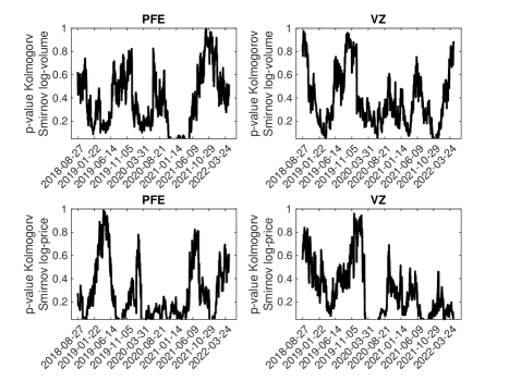
Figure 4.1: Kolmogorov-Smirnov test applied to the log-volume (upper panels) and log-price (lower panels) for PFE and VZ stocks, with the null hypothesis assuming normality of the time series. The $y$-axis range spans from $0.05$ to $1$.

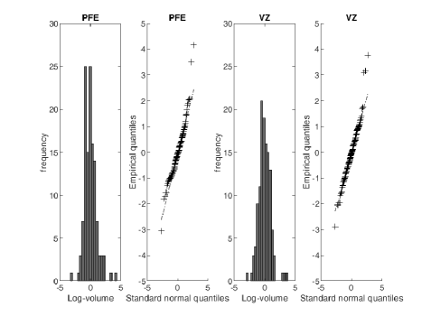
Figure 4.2: Frequency histogram and QQ-plot of the standardized daily log volumes (from February 28th, 2018, to April 28th, 2022).

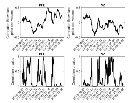
Figure 4.3: Correlation coefficients between price and volume time series (top panels) and the corresponding p-values (bottom panels).

Figure 4.2 shows the frequency histogram and the QQ-plot of the standardized daily log-volumes relative to the time period considered and it confirms that the observed total trading volume follows a GBM.

Figure 4.3 shows the estimated Pearson correlation coefficients of price and volume and the corresponding $p-value$. Figure 4.3 shows that we cannot reject the null hypothesis of zero correlation in several windows. This confirms that two different Brownian processes drive the dynamics of price and volume.

We additionally assess the robustness of the results by employing the estimated noises and parameters to generate one-day-ahead price forecasts. In Figure 4.4, the true prices are represented by dashed bold lines, while the simulated prices are depicted by solid lines for both the PFE stock (left panel) and the VZ stock (right panel). The overlapping curves indicate the reliability of the estimated parameters.

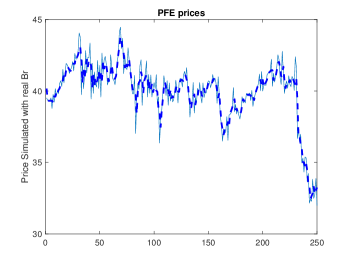
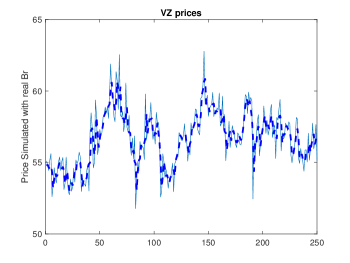
Figure 4.4: One-day-ahead forecasts (solid line) and observed values (dashed bold line) for PFE (left panel) and VZ (right panel).

Now, we show the estimated relevant quantities, that is the ratio drift-to-diffusion, i.e. $\psi_{t}/\sigma_{t}$, of the volume time series compared with the theoretical ratio prescribed by Merton, $(\mu_{t}-r-\sigma_{t}^{2})/\sigma_{t}$ (Fig. 4.5), the volume and market price of risk (Fig. 4.6) and the observed trading rate (Fig. 4.7).

Using the estimates $\hat{\mu}_{t}$ and $\hat{\sigma}_{t}$ of $\mu_{t}$ and $\sigma_{t}$, respectively, we compute the theoretical ratio using ${\rm ratio}_{th}=(\hat{\mu}_{t}-r-\hat{\sigma}^{2}_{t})/\hat{\sigma}_{t}$. Analogously, using the estimates $\hat{\mu}_{v}\approx\eta_{t}\psi_{t}$ and $\hat{\sigma}_{v}\approx\eta_{t}\sigma_{t},$ we compute the drift-to-diffusion ratio:

$$\textrm{\rm ratio}_{obs}=\frac{\hat{\mu}_{v}}{\hat{\sigma}_{v}}.$$ (42)

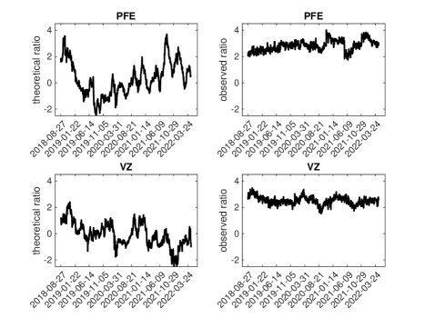
Figure 4.5: Comparison of Merton’s theoretical drift-to-diffusion ratio with observed values of the ratio in volume time series. Linear regression with intercept only: PFE – Intercept = 2.82, Standard deviation = 0.0132; VZ – Intercept = 2.51, Standard deviation = 0.0099.

Upon examining Figure 4.5, it is evident that the observed ratio does not coincides with the Merton theoretical ratio. More interestingly, the observed ratio is approximately constant in the time period considered and its range spans 2–4. This intriguing result appears to confirm the experiment outlined in Kahneman and Tversky (1991) [12], who demonstrated that individuals tend to accept a bet over a certain monetary value only if the potential win is at least 2.5 times higher. We check the value of the observed ratio by performing linear regression with intercept only, yielding the following results: PFE intercept equal to 2.82 with standard deviation 0.0132; VZ intercept equal to 2.51 with standard deviation is 0.0099. These results are inline with the experiment of Kahneman and Tversky (1991) [12].

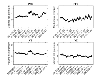
Figure 4.6: Volume risk premium, $\psi_{t}+\rho\sigma_{t}^{2}$ (first column, left panels), and the volume price of risk, $(\psi+\rho\sigma_{t}^{2})/\sigma_{t}$ (first column, right panels). The market risk premium and price of risk are in second columns of left and right panels respectively.

In the left panels of Figure 4.6 we compare the volume risk premium, $\psi_{t}+\rho_{t}\sigma_{t}^{2}$, (first column – left panels) with the market risk premium, $\mu_{t}-r$ (second column – left panels) while the right panels show the volume price of risk, $(\psi+\rho_{t}\sigma_{t}^{2})/\sigma_{t}$ (first column – right panels) and the market price of risk, $(\mu_{t}-r)/\sigma_{t}$ (first column – right panels).

Notably, the volume price of risk remains relatively constant. Conducting linear regression with intercept only yields the following results: PFE intercept equals 2.84 with a standard deviation of 0.014, while VZ intercept equals 2.49 with a standard deviation of 0.01.

Regarding the market price of risk, we find an intercept of 0.549 with a standard deviation of 0.041 for PFE, and an intercept of 0.0914 with a standard deviation of 0.02 for VZ.

The volume price of risk can be easily interpreted from a behavioral standpoint. Investors trading Pfizer stock, both pre-Covid and post-Covid, face slightly higher risks compared to those trading a more stable stock like Verizon Communications. Consequently, to participate in this market rather than sticking to bonds, they demand a premium per unit of risk of approximately three times the risk they face.

The interpretation of the market price of risk is straightforward from a comparative perspective, as the price for investing in PFE is approximately five times larger than investing in VZ. However, interpreting this in terms of a bet, as outlined by Kahneman and Tversky (1991) [12], is challenging because a price of one half is meaningless in this framework.

Finally, we turn our attention to the “ideal Merton world” scenario, where the discounted trading strategy reduces to a martingale with a trading price of risk (denoted as $\varphi_{t}$) equal to the expression (41), i.e. ${\varphi_{t}}=\left(\mu_{t}-r+(\psi_{t}+\rho_{t}\sigma_{t}^{2})\eta_{t}\right)/(\sigma_{t}\sqrt{1+\eta_{t}^{2}+2\rho\eta_{t}})$. This trading price of risk incorporates both the price risk and the volume risk associated with the trading rate, $\eta_{t}$. Specifically, when the trading rate is small, the price of risk reduces to the market price of risk. However, larger trading rates may result in an increase in the price of risk, potentially exceeding the volume price of risk.

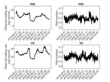
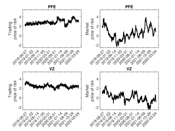
Figure 4.7: Trading rate and risk aversion (left panels); trading price of risk and market price of risk (right panels).

In Figure 4.7, the left panels display the estimated trading rate $\eta_{t}$ and risk aversion $\mu_{\gamma_{t}}$, while the right panels show the trading price of risk and market price of risk. We conducted linear regression with intercept only for risk aversion, trading price of risk, and market price of risk, yielding the following results:

1. PFE
   Risk aversion intercept = 0.491 with standard deviation 0.00135;
   Trading price of risk intercept=2.869 with standard deviation 0.0149;
   Market price of risk intercept =0.549 with standard deviation 0.041;

2. VZ
   Risk aversion intercept = 0.499 with standard deviation 0.00139;
   Trading price of risk intercept=2.489 with standard deviation 0.0105;
   Market price of risk intercept =0.0914 with standard deviation 0.02.

We observe that the trading price of risk closely resembles the volume price of risk and is consistent with the findings of Kahneman and Tversky (1991) [12]. It is remarkable how the risk aversion remains constant over time for traders operating in these assets.

4.2 Market Indices

In this section we analyze two market indices, S&P 500 (SPX) and NASDAQ (NA), from September 17th, 2018, to September 15th, 2023. We repeat the experiment of Section 4.1.

Figure 4.8 displays the p-values (on the $y$-axis) obtained from the Kolmogorov-Smirnov test, where the null hypothesis assumes normality of the time series. This test is applied to both the log-volume (upper panels) and the log-price (lower panels) for S&P 500 and NasdAQ within each window utilized in the estimation process. The $y$-axis ranges from 0.05 to 1.

We observe that the p-values for the log-volume are generally greater than or equal to 0.05 for several dates, except during the Covid period. However, the volume of the SPX index exhibits a worse behavior compared to that of the NA index. Regarding the prices, normality is particularly rejected during the Covid years (2020-2021) for both the SPX and NA prices.

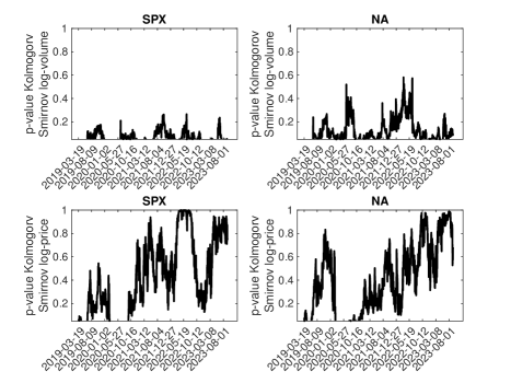
Figure 4.8: Kolmogorov-Smirnov test applied to the log-volume (upper panels) and log-price (lower panels) for SPX and NA indices, with the null hypothesis assuming normality of the time series. The $y$-axis range spans from $0.05$ to $1$.

Figure 4.9 shows the frequency histogram and the QQ-plot of the standardized daily log-volumes relative to the time period considered and it confirms that the observed total trading volume follows a GBM.

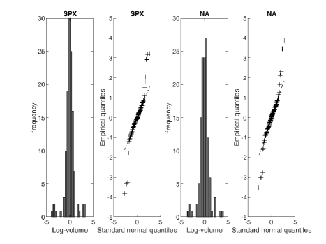
Figure 4.9: Frequency histogram and QQ-plot of the standardized daily log volumes (from September 17th, 2018, to September 15th, 2023).

Figure 4.10 shows the estimated Pearson correlation coefficients of price and volume and the corresponding $p-value$.

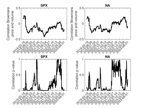
Figure 4.10: Correlation coefficients between price and volume time series (top panels) and the corresponding p-values (bottom panels).

Figure 4.10 indicates that we cannot reject the null hypothesis of zero correlation in several windows. This suggests that two distinct Brownian motions drive the dynamics of price and volume.

We additionally assess the robustness of the results by employing the estimated noises and parameters to generate one-day-ahead price forecasts. In Figure 4.11, the true prices are represented by dashed bold lines, while the simulated values are indicated by solid lines for both the SPX index (left panel) and the NA index (right panel). The overlapping curves indicate the reliability of the estimated parameters.

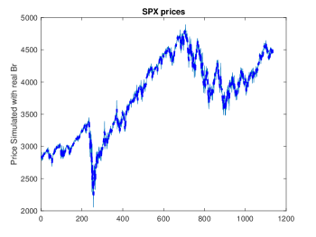
Figure 4.11: One-day-ahead forecasts (solid line) and observed values (dashed bold line) for SPX (left panel) and NA (right panel).

Next, we analyze the estimates of the ratio of drift-to-diffusion, denoted as $\psi_{t}/\sigma_{t}$, and compare them with the ratio prescribed by Merton, $(\mu_{t}-r-\sigma_{t}^{2})/\sigma_{t}$ (see Fig. 4.12). Additionally, we examine the volume price of risk and the market price of risk (Fig. 4.13), along with the observed trading rate (Fig. 4.14).

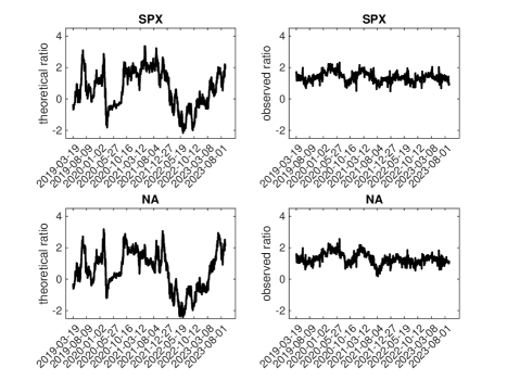
Figure 4.12: Comparison of Merton’s theoretical drift-to-diffusion ratio with observed values of the ratio in volume time series. Linear regression with intercept only: SPX – Intercept = 1.38, Standard deviation = 0.00845; NA – Intercept = 1.28, Standard deviation = 0.0102.

Upon examining Figure 4.12, it is evident that the observed ratio does not coincide with the Merton theoretical ratio. More interestingly, the observed ratio remains approximately constant throughout the considered time period, ranging from 0.5 to 2.5.

We further assess the value of the observed ratio by conducting linear regression with intercept only, resulting in the following outcomes: SPX intercept equals 1.38 with a standard deviation of 0.00845, and NA intercept equals 1.28 with a standard deviation of 0.0102.

These results are coherent with the fact that PFE and VZ stocks are riskier than the SPX and NA indices. Specifically, the ratios of the indices are half those of the stocks.

In the left panels of Figure 4.13 we compare the volume risk premium, $\psi_{t}+\rho_{t}\sigma_{t}^{2}$, (first column – left panels) with the market risk premium, $\mu_{t}-r$ (second column – left panels) while the right panels show the volume price of risk, $(\psi+\rho_{t}\sigma_{t}^{2})/\sigma_{t}$ (first column – right panels) and the market price of risk, $(\mu_{t}-r)/\sigma_{t}$ (first column – right panels).

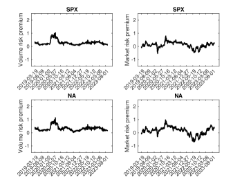
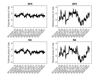
Figure 4.13: Volume risk premium, $\psi_{t}+\rho\sigma_{t}^{2}$ (first column, left panels), and the volume price of risk, $(\psi+\rho\sigma_{t}^{2})/\sigma_{t}$ (first column, right panels). The market risk premium and price of risk are in second columns of left and right panels respectively.

Notably, the volume price of risk remains relatively constant. Conducting linear regression with intercept only yields the following results: SPX intercept equals 1.36 with a standard deviation of 0.0084, while NA intercept equals 1.27 with a standard deviation of 0.01.

Regarding the market price of risk, we find an intercept of 0.844 with a standard deviation of 0.034 for PFE, and an intercept of 0.807 with a standard deviation of 0.035 for NA.

The volume price of risk indicates that investors trading Pfizer or Verizon stocks face slightly higher risks compared to those trading SPX and NA indices. By comparing the volume price of risk, we can conclude that investors participating in the stock market rather than sticking to market indices demand a premium per unit of risk of approximately twice as high.

In contrast, the market price of risk for the indices remains substantially the same and comparable to those of the considered stocks.

Finally, we turn our attention to the trading price of risk in the “ideal Merton world”.

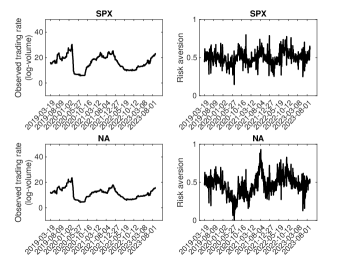
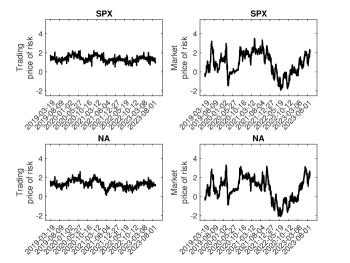
Figure 4.14: Trading rate and risk aversion (left panels); trading price of risk and market price of risk (right panels).

In Figure 4.14, the left panels display the estimated trading rate $\eta_{t}$ and risk aversion $\mu_{\gamma_{t}}$, while the right panels show the trading price of risk and market price of risk. We conducted linear regression with intercept only for risk aversion, trading price of risk, and market price of risk, yielding the following results:

1. SPX
   Risk aversion intercept = 0.499 with standard deviation 0.0023;
   Trading price of risk intercept=1.3826 with standard deviation 0.0081;
   Market price of risk intercept =0.8439 with standard deviation 0.0340;

2. NA
   Risk aversion intercept = 0.466 with standard deviation 0.00384;
   Trading price of risk intercept=1.3211 with standard deviation 0.0107;
   Market price of risk intercept =0.0807 with standard deviation 0.0354.

We observe that the trading price of risk closely resembles the volume price of risk and is consistent with the findings of Kahneman and Tversky (1991) [12]. It is remarkable how the risk aversion remains constant over time for traders operating in these assets.

4.3 Exchange rates: BTC-USD and EUR-USD

In this section we analyze two exchange rates, Bitcoin to US Dollar (BTC-USD or BTC for short) and Euro to US-Dollar (EUR-USD or EUR for short), from September 30th, 2018, to September 23rd, 2023. Also in this case we repeat the experiment of Section 4.1.

Figure 4.15 displays the p-values (on the $y$-axis) obtained from the Kolmogorov-Smirnov test, where the null hypothesis assumes normality of the time series. This test is applied to both the log-volume (upper panels) and the log-price (lower panels) for BTC-USD and EUR-USD within each window used in the estimation process. As in the previous sections, the $y$-axis ranges from 0.05 to 1.

We observe that the p-values for the log-volume and log-rate of BTC-EUR are generally greater than or equal to 0.05 for several dates, except during the post Covid period (2021). THe EUR-USD rate reject the model for both volume and rate. Thus, the results regarding the EUR-USD exchange rates could be not reliable.

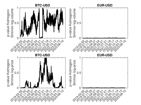
Figure 4.15: Kolmogorov-Smirnov test applied to the log-volume (upper panels) and log-price (lower panels) for BTC and EUR rates, with the null hypothesis assuming normality of the time series. The $y$-axis range spans from $0.05$ to $1$.

Figure 4.16 shows the frequency histogram and the QQ-plot of the standardized daily log-volumes relative to the time period considered and it confirms that the observed total trading volume follows a GBM.

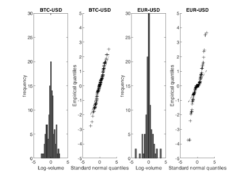
Figure 4.16: Frequency histogram and QQ-plot of the standardized daily log volumes (from September 30th, 2018, to September 23rd, 2023).

Figure 4.17 shows the estimated Pearson correlation coefficients of price and volume and the corresponding $p-value$.

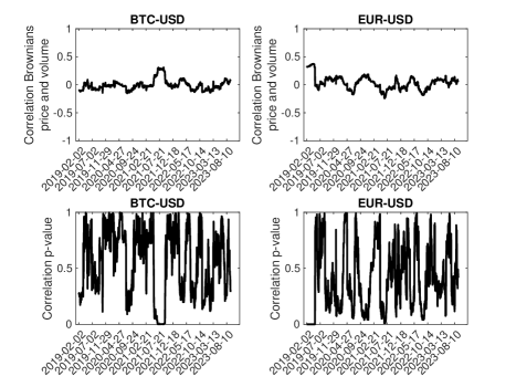
Figure 4.17: Correlation coefficients between price and volume time series (top panels) and the corresponding p-values (bottom panels).

Figure 4.17 indicates that we cannot reject the null hypothesis of zero correlation in several windows. This suggests that two distinct Brownian motions drive the dynamics of price and volume.

As in the previous sections, we perform an analysis of the robustness by employing the estimated noises and parameters to generate one-day-ahead price forecasts. In Figure 4.18, the true exchange rates are represented by dashed bold lines, while the simulated values are indicated by solid lines for both BTC-USD (left panel) and EUR-USD index (right panel). The overlapping curves indicate the reliability of the estimated parameters.

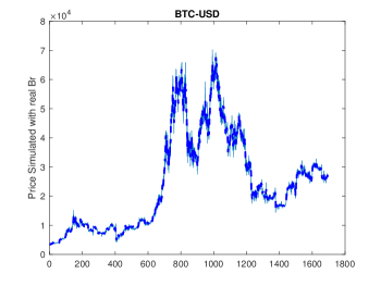
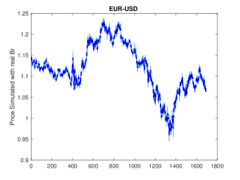
Figure 4.18: One-day-ahead forecasts (solid line) and observed values (dashed bold line) for BTC-USD (left panel) and EUR-USD (right panel).

Next, we analyze the estimates of the ratio of drift-to-diffusion, denoted as $\psi_{t}/\sigma_{t}$, and compare them with the ratio prescribed by Merton, $(\mu_{t}-r-\sigma_{t}^{2})/\sigma_{t}$ (see Fig. 4.19). Additionally, we examine the volume price of risk and the market price of risk (Fig. 4.20), along with the observed trading rate (Fig. 4.21).

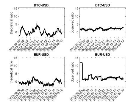
Figure 4.19: Comparison of Merton’s theoretical drift-to-diffusion ratio with observed values of the ratio in volume time series. Linear regression with intercept only: BTC – Intercept = 2.03, Standard deviation = 0.013; EUR – Intercept = 2.81, Standard deviation = 0.057.

Upon examining Figure 4.19, it is evident that the observed ratio does not coincide with the Merton theoretical ratio. More interestingly, the observed ratio remains approximately constant throughout the considered time period, ranging from 1.5 to 3.0.

We further assess the value of the observed ratio by conducting linear regression with intercept only, resulting in the following outcomes: BTC intercept equals 2.03 with a standard deviation of 0.013, and EUR intercept equals 2.81 with a standard deviation of 0.0567.

The drift-to-diffusion ratios are comparable with the ratios of PFE and VZ stocks rather than with those of the SPX and NA indices.

In the left panels of Figure 4.20 we compare the volume risk premium, $\psi_{t}+\rho_{t}\sigma_{t}^{2}$, (first column – left panels) with the market risk premium, $\mu_{t}-r$ (second column – left panels) while the right panels show the volume price of risk, $(\psi+\rho_{t}\sigma_{t}^{2})/\sigma_{t}$ (first column – right panels) and the market price of risk, $(\mu_{t}-r)/\sigma_{t}$ (first column – right panels).

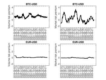
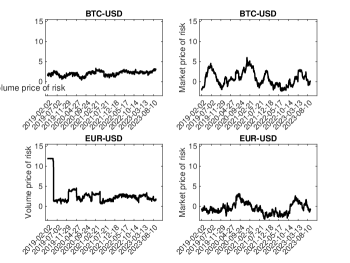
Figure 4.20: Volume risk premium, $\psi_{t}+\rho_{t}\sigma_{t}^{2}$ (first column, left panels), and the volume price of risk, $(\psi+\rho_{t}\sigma_{t}^{2})/\sigma_{t}$ (first column, right panels). The market risk premium and price of risk are in second columns of left and right panels respectively.

Conducting a linear regression with intercept only yields the following results: the intercept for BTC-USD is 2.03 with a standard deviation of 0.013, while for EUR-USD, it is 2.981 with a standard deviation of 0.0567. Surprisingly, the reward for investing in BTC rather than EUR appears to be lower.

Regarding the market price of risk, we find an intercept of 0.7645 with a standard deviation of 0.0428 for the BTC-USD rate, and an intercept of -0.461 with a standard deviation of 0.032 for EUR-USD. The negative market price of risk for the EUR-USD exchange rate is consistent with the findings of the European Commission’s Directorate General for Economic and Financial Affairs, as presented in their report on Euro-US Dollar Exchange Rate Dynamics (see specifically page 9: https://economy-finance.ec.europa.eu/system/files/2020-11/eb055_en.pdf).

The volume price of risk indicates that investors trading Pfizer or Verizon stocks face slightly higher risks compared to those trading SPX and NA indices. By comparing the volume price of risk, we can conclude that investors participating in the stock market rather than sticking to market indices demand a premium per unit of risk of approximately twice as high.

In contrast, the market price of risk for the indices remains substantially the same and comparable to those of the considered stocks.

Finally, we turn our attention to the trading price of risk in the “ideal Merton world”.

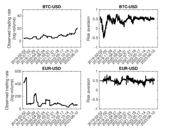
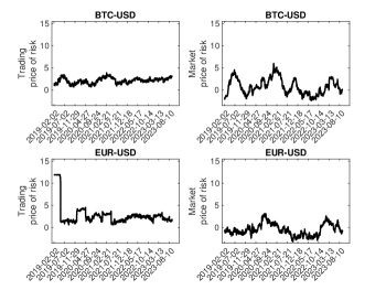
Figure 4.21: Trading rate and risk aversion (left panels); trading price of risk and market price of risk (right panels).

In Figure 4.21, the left panels display the estimated trading rate $\eta_{t}$ and risk aversion $\mu_{\gamma_{t}}$, while the right panels show the trading price of risk and market price of risk. We conducted linear regression with intercept only for risk aversion, trading price of risk, and market price of risk, yielding the following results:

1. BTC-USD
   Risk aversion intercept = 0.436 with standard deviation 0.00496;
   Trading price of risk intercept=2.1303 with standard deviation 0.01476;
   Market price of risk intercept =0.7645 with standard deviation 0.0428;

2. EUR-USD
   Risk aversion intercept = 0.502 with standard deviation 0.002184;
   Trading price of risk intercept=2.805 with standard deviation 0.0568;
   Market price of risk intercept =-0.461 with standard deviation 0.0318.

We note that the trading price of risk closely resembles the volume price of risk, consistent with the findings of Kahneman and Tversky (1991) [12]. It is noteworthy how risk aversion remains relatively constant over time for traders operating in these assets. What is particularly surprising is the negative market price of risk for the EUR-USD exchange rate. However, as previously mentioned, this finding aligns with the results of the European Commission’s Directorate General for Economic and Financial Affairs regarding Euro-US Dollar Exchange Rate Dynamics (refer to page 9 of the report: https://economy-finance.ec.europa.eu/system/files/2020-11/eb055_en.pdf).

4.4 Empirical analysis over a long horizon

Let us conclude the empirical analysis by examining the trading rate, risk aversion, and relevant risks (i.e., market price of risk, trading price of risk) over extended periods, including the very beginning of the asset.

We conducted analyses using daily price data for Pfizer from June 2nd, 1972, to May 26th, 2023, Verizon Communications from November 21st, 1983, to May 26th, 2023, the S&P 500 from January 3rd, 1950, to April 8th, 2024, and BTC-USD from September 17th, 2014, to April 8th, 2024. We estimate the parameters using four years of daily data. Despite differing time spans, the results offer a unified interpretation, which we will elaborate on.

Figures 4.22 and 4.23 provide empirical evidence that in the initial phases of an asset’s life, the reward required for the investment risk is higher than 2-2.5, with the exception of the SPX index. However, risk aversion remains substantially constant at 0.5, except for the BTC-USD rate. In contrast, the market price of risk fluctuates for all the assets analyzed.

Interestingly, the trading price of risk serves as a measure of potential asset growth or investor trust in the asset. Higher values of the trading price of risk indicate lower investor trust but higher potential growth for the asset. Values of the trading risk higher than 2.5 may indicate that the stock is not well-established.

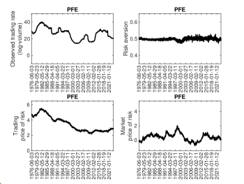
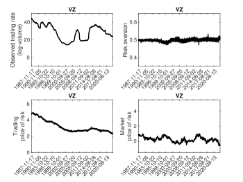
Figure 4.22: Upper panels: trading rate (left) and risk aversion (right); Left panels: trading price of risk (left) and market price of risk (right) for PFE (left panels) and VZ (right panels)

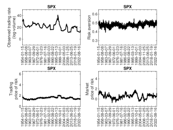
Figure 4.23: Upper panels: trading rate (left) and risk aversion (right); Left panels: trading price of risk (left) and market price of risk (right).

In fact, Pfizer and Verizon Communications trading price of risk looks like a decreasing function of time while the trading price of risk of the exchange rate BTU-USD decreases and achieve its minimum in November 2020 and, then, re-start to increase by achieving a value approximately of 2. This is probably due to the bitcoin halving phenomenon. The bitcoin trading reveals a risk aversion less than 0.5 up to today. Finally, the S&P 500 index show a value which is approximately 2. This denotes a very well established asset.

References

- [1] Borgonovo, E. , Cillo, A., Caselli, S. Masciandaro, D. (2018). Between Cash, Deposit and Bitcoin: Would We Like a Central Bank Digital Currency? Money Demand and Experimental Economics. BAFFI CAREFIN Centre Research Paper No. 2018-75, available at SSRN: https://ssrn.com/abstract=3160752 or http://dx.doi.org/10.2139/ssrn.3160752
- [2] Borgonovo, E. , Cillo, A., Caselli, S. Masciandaro, D. Rabitti, G. (2019). Privacy and Money: It Matters. BAFFI CAREFIN Centre Research Paper No. 2019-108, available at SSRN: https://ssrn.com/abstract=3330494 or http://dx.doi.org/10.2139/ssrn.3330494)
- [3] Bouchaud, J. P. (2017). Price Impact. Encyclopedia of Quantitative Finance, doi: 10.1002/9780470061602.eqf18006
- [4] Dai, M., Dong, Y., Jia, Y., Zhou, X. Y. (2023). Learning Merton’s Strategies in an Incomplete Market: Recursive Entropy Regularization and Biased Gaussian Exploration, arXiv:2312.11797
- [5] Carmona, R. Webster, K. T. (2013). The Self-Financing Equation in High Frequency Markets. Available at SSRN: https://ssrn.com/abstract=2365122 or http://dx.doi.org/10.2139/ssrn.2365122
- [6] Chebbi, S., Soner, H.M. (2013). Merton problem in a discrete market with frictions. Nonlinear Analysis: Real World Applications, 14 (1), 179–187.
- [7] Chebbi, S., Ounaies, S. (2023). Optimal investment of Merton model for multiple investors with frictions. Mathematics, 11 (13), 2873 .
- [8] Chen, T. (2019). The price impact of trade-size clustering: Evidence from an intraday analysis. Journal of Business Research 101, 300–314.
- [9] Gatheral, J. (2010). No-dynamic-arbitrage and market impact. Quantitative Finance, 10(7), 749–759.
- [10] He, H., Mamaysky, H. (2005). Dynamic trading policies with price impact. Journal of Economic Dynamics and Control, 29 (5), 891–930.
- [11] Kahneman, D., Tversky, A. (1979). Prospect Theory: An Analysis of Decision under Risk. Econometrica 47 (2), 263–292.
- [12] Kahneman, D., Tversky, A. (1991). Loss Aversion in Riskless Choice: A Reference-Dependent Model. The Quarterly Journal of Economics 106 (4), 1039–1061.
- [13] Levy, M. (2010). Loss aversion and the price of risk. Quantitative Finance, 10 (9), 1009–1022.
- [14] Lou, X., Shu, T. (2017). Price Impact or Trading Volume. The Review of Financial Studies 30(12), 4481–4520.
- [15] Le Van, C., Dana, R.-A. (2003). Dynamic Programming in Economics, Kluer Academic Publishers: Norwell, MA, USA.
- [16] Mariani, F., Recchioni, M.C., Ciommi, M. (2019). Merton’s portfolio problem including market frictions: A closed form formula supporting the shadow price approach. European Journal of Operational Research, 275 (3), 1178–1189.