Weighted average temperature as the effective temperature of a system in contact with two thermal baths

Abstract

We investigate the effective temperature of a harmonic chain whose two ends are coupled to two baths at different temperatures. We propose to take the weighted average temperature as the effective temperature of the system. The weight factors are related to the couplings between the system and two baths as well as the asymmetry of interactions between oscillators. We revisit the thermodynamics of nonequilibrium steady states based on the weighted average temperature. It is found that the fundamental thermodynamic relations in nonequilibrium steady states possess similar concise forms as those in equilibrium thermodynamics, provided that we replace the temperature in equilibrium with the weighted average temperature in steady states. We also illustrate the procedure to calculate the effective temperatures via four examples.

I Introduction

Thermodynamics was regarded as a universal theory by Einstein [1]: `It is the only physical theory of universal content, which I am convinced, that within the framework of applicability of its basic concepts will never be overthrown.' The whole theoretical system of thermodynamics is on the basis of four laws of thermodynamics. Temperature is a core concept for the zeroth law of thermodynamics, which characterizes an equilibrium state. However, this concept cannot be directly extended to general nonequilibrium states since the transitivity of thermal equilibrium is broken out of equilibrium. McLennan stated: `Nonequilibrium temperature is introduced for theoretical convenience rather than to take advantage of a basic principle' [2]. Different definitions of nonequilibrium temperatures such as kinetic temperature, local temperature, effective temperature have been proposed in various situations involving from passive to active, classic to quantum systems [3, 4, 5, 6, 7, 8, 9, 10, 11, 12, 13, 14, 15, 16, 17, 18, 19, 20].

Although the definition of nonequilibrium temperature is controversial, researchers still believe that effective temperature may be well defined for steady-state systems in contact with two thermal baths at different temperatures. There are two main viewpoints on effective temperatures of these systems in literature: (i) the mean temperature; (ii) the weighted average temperature. The mean temperature is a natural definition of effective temperature for a system in contact with two thermal baths at different temperatures. Parrondo and Español considered an axle with vanes at both ends symmetrically coupled to two thermal baths, and found that the steady state can be described as the Boltzmann canonical distribution with an effective temperature being the arithmetical mean of temperatures of two baths [21]. In recent remarkable work by Wu and Wang [22], the nonequilibrium equation of state of a harmonic chain coupled to two thermal baths was established, which is divided into two parts: One has the form of the equilibrium equation of state with the equilibrium temperature replaced by the mean temperature of two baths; the other depends on the temperature difference between two baths. For a finite-size quantum system connected to two thermal and particle reservoirs, the nonequilibrium density matrix was derived by Ness, which is given by a generalized Gibbs-like ensemble with an effective reciprocal temperature being the mean of reciprocal temperatures of two baths [23].

If the system is asymmetrically coupled to two thermal baths, the weighted average temperature may be regarded as a more reasonable definition of effective temperature. Van den Broeck et al. investigated the heat transfer by a shared piston simultaneously in contact with two thermal baths at different temperatures [24]. They found that the steady state is described by a canonical distribution with an effective temperature being the weighted average of temperatures of two baths. The weight factors are related to frictional coefficients of the piston in both baths. The idea of weighted average temperature holds also for underdamped Langevin systems in contact with multiple reservoirs [25, 26] and quantum heat transfers at the nanoscale [27]. Sheng and the author in the present paper also suggested the weighted average reciprocal temperature as the inverse effective temperature of finite-time heat engines, the devices outputting work and absorbing heat simultaneously [28]. The weighted average temperatures mentioned above are introduced for simple systems with few degrees of freedom. We may ask: whether can we give a unified definition and calculation procedure of effective temperature in steady state via weighted average temperature for a system with multiple degrees of freedom? Can the fundamental relations in equilibrium thermodynamics be extended to nonequilibrium steady states? Do the extended relations possess the same forms as those in equilibrium thermodynamics? Aiming at these questions, we will develop the idea of weighted average temperature based on a model of harmonic chain coupled to two thermal baths. We will try to give a unified definition of effective temperature and then revisit thermodynamics of nonequilbrium steady states via the weighted average temperature. The rest of this paper is organized as follows. In Sec. II, we present a minimal model which consists of a harmonic chain with its two ends coupled to two thermal baths at different temperatures. In Sec. III, we propose a definition of effective temperature with the weighted average temperature. In Sec. IV, we revisit thermodynamics of nonequilibrium steady states by taking the weighted average temperature as the effective temperature. In Sec. V, we discuss four examples and calculate the corresponding effective temperatures. The last section is a brief summary and discussion.

II Model system: a harmonic chain coupled to two thermal baths

The model system that we considered is a harmonic chain coupled to two thermal baths as shown in Fig. 1. The chain consists of $N$ particles and $N+1$ elastic springs. Particle 1 is coupled to a thermal bath at temperature $T_{L}$, and particle $N$ is in contact with a thermal bath at temperature $T_{R}$. The equations of motion of particle $i$ ($i=1,2,3,\cdots,N$) may be expressed as the Langevin dynamics:

$$\frac{dx_{i}}{dt} = {p_{i}},$$ (1)

$$\frac{dp_{i}}{dt} = -\bar{k}_{i-1}x_{i-1}-k_{i}x_{i}-\bar{k}_{i}x_{i+1}$$ (2)

$$+ [-\gamma_{L}p_{1}+\xi_{L}(t)]\delta_{i1}+[-\gamma_{R}p_{N}+\xi_{R}(t)]\delta_{iN},$$

where $x_{i}$ and $p_{i}$ represent the coordinate and momentum of particle $i$, respectively. In Eq. (1), we have assumed that all particles are of the same mass which is set to be unit for simplicity. In Eq. (2), $k_{i}$ and $\bar{k}_{i}$ are related to the elastic constants of the springs. We have imposed $\bar{k}_{0}=\bar{k}_{N}=0$. $\delta_{i1}$ and $\delta_{iN}$ are the Kronecker delta notations. $\gamma_{L}$ and $\gamma_{R}$ represent frictional coefficients of particles 1 and $N$, respectively. $\xi_{L}(t)$ and $\xi_{R}(t)$ are white noises due to the thermal baths which satisfy $\langle\xi_{\alpha}(t)\rangle=0$ and $\langle\xi_{\alpha}(t)\xi_{\alpha}(t^{\prime})\rangle=\gamma_{\alpha}k_{B}T_{\alpha}\delta(t-t^{\prime})$ with $\alpha=L$ or $R$. $k_{B}$ is the Boltzmann constant which is set to be unit in the following discussions.

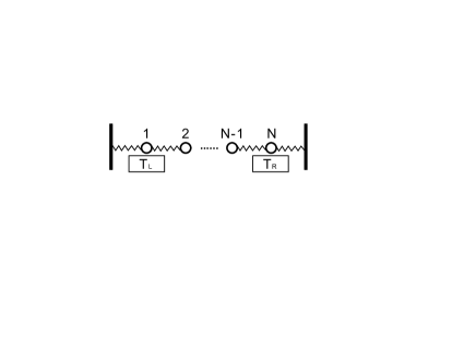
Figure 1: A harmonic chain with its two ends coupled to two thermal baths at different temperatures $T_{L}$ and $T_{R}$.

Introduce position vector $\mathbf{x}=[x_{1},x_{2},\cdots,x_{N}]^{\mathrm{T}}$, momentum vector $\mathbf{p}=[p_{1},p_{2},\cdots,p_{N}]^{\mathrm{T}}$, phase vector $\mathbf{z}=[x_{1},x_{2},\cdots,x_{N},p_{1},p_{2},\cdots,p_{N}]^{\mathrm{T}}$, and noise vector $\bm{\xi}=[0,0,\cdots,0,\xi_{1},0\cdots,0,\xi_{N}]^{\mathrm{T}}$. In the whole paper, the superindex $\mathrm{T}$ represents the transpose of a matrix. Introduce $N\times N$-order elastic matrix

$$\mathbf{K}=\left[\begin{array}[]{cccccc}k_{1}&\bar{k}_{1}&0&0&\cdots&0\\ \bar{k}_{1}&k_{2}&\bar{k}_{2}&0&\cdots&0\\ 0&\bar{k}_{2}&k_{3}&\bar{k}_{3}&\cdots&0\\ \vdots&\ddots&\ddots&\ddots&\ddots&\vdots\\ 0&\cdots&0&\bar{k}_{N-2}&k_{N-1}&\bar{k}_{N-1}\\ 0&0&\cdots&0&\bar{k}_{N-1}&k_{N}\end{array}\right],$$ (3)

and frictional matrix

$$\bm{\Gamma}=\left[\begin{array}[]{ccccc}\gamma_{L}&0&\cdots&0&0\\ 0&0&\cdots&0&0\\ \vdots&\vdots&\ddots&\vdots&\vdots\\ 0&0&\cdots&0&0\\ 0&0&\cdots&0&\gamma_{R}\end{array}\right].$$ (4)

Then the equations of motion of the system may be transformed into a matrix form:

$$\frac{d\mathbf{z}}{dt}=-\mathbf{A}\mathbf{z}+\bm{\xi},$$ (5)

where coefficient matrix

$$\mathbf{A}=\left[\begin{array}[]{cc}\mathbf{0}&-\mathbf{I}\\ \mathbf{K}&\bm{\Gamma}\end{array}\right]$$ (6)

with $\mathbf{0}$ and $\mathbf{I}$ being $N\times N$-order zero matrix and identity matrix, respectively.

Introduce steady-state covariance matrices $\bm{\sigma}_{xx}=\langle\mathbf{x}\mathbf{x}^{\mathrm{T}}\rangle_{t\rightarrow\infty}$, $\bm{\sigma}_{xp}=\langle\mathbf{x}\mathbf{p}^{\mathrm{T}}\rangle_{t\rightarrow\infty}$, $\bm{\sigma}_{px}=\langle\mathbf{p}\mathbf{x}^{\mathrm{T}}\rangle_{t\rightarrow\infty}$, $\bm{\sigma}_{pp}=\langle\mathbf{p}\mathbf{p}^{\mathrm{T}}\rangle_{t\rightarrow\infty}$, and $\bm{\sigma}=\langle\mathbf{z}\mathbf{z}^{\mathrm{T}}\rangle_{t\rightarrow\infty}=\left[\begin{array}[]{cc}\bm{\sigma}_{xx}&\bm{\sigma}_{xp}\\ \bm{\sigma}_{px}&\bm{\sigma}_{pp}\end{array}\right]$. Covariance matrix $\bm{\sigma}$ is symmetrical, which implies $\bm{\sigma}_{xx}^{\mathrm{T}}=\bm{\sigma}_{xx}$, $\bm{\sigma}_{pp}^{\mathrm{T}}=\bm{\sigma}_{pp}$ and $\bm{\sigma}_{xp}^{\mathrm{T}}=\bm{\sigma}_{px}$.

Since Eq. (5) describes an Ornstein-Uhlenbeck process, the covariance matrix satisfies the continuous-time Lyapunov equation [5, 22, 29, 30]:

$$\mathbf{A}\bm{\sigma}+\bm{\sigma}\mathbf{A}^{\mathrm{T}}=2\mathbf{D}_{\mathrm{t}},$$ (7)

where $\mathbf{D}_{\mathrm{t}}=\left[\begin{array}[]{cc}\mathbf{0}&\mathbf{0}\\ \mathbf{0}&\mathbf{D}\end{array}\right]$. $\mathbf{D}$ is $N\times N$-order diffusion matrix which is explicitly expressed as

$$\mathbf{D}=\left[\begin{array}[]{ccccc}\gamma_{L}T_{L}&0&\cdots&0&0\\ 0&0&\cdots&0&0\\ \vdots&\vdots&\ddots&\vdots&\vdots\\ 0&0&\cdots&0&0\\ 0&0&\cdots&0&\gamma_{R}T_{R}\end{array}\right].$$ (8)

III Weighted average temperature

In this section, we will propose a definition of effective temperature via the weighted average of temperatures $T_{L}$ and $T_{R}$.

If $T_{L}=T_{R}=T$, the system reaches an equilibrium state where $\bm{\sigma}_{xx}\mathbf{K}=\bm{\sigma}_{pp}=T\mathbf{I}$. With the consideration of this point, we introduce $\tilde{\mathbf{K}}=\left[\begin{array}[]{ll}\mathbf{K}&\mathbf{0}\\ \mathbf{0}&\mathbf{I}\end{array}\right]$ and define revised covariance matrix

$$\tilde{\bm{\sigma}}={\bm{\sigma}}\tilde{\mathbf{K}}=\left[\begin{array}[]{ll}\bm{\sigma}_{xx}\mathbf{K}&\bm{\sigma}_{xp}\\ \bm{\sigma}_{px}\mathbf{K}&\bm{\sigma}_{pp}\end{array}\right]$$ (9)

such that equilibrium covariance matrix $\tilde{\bm{\sigma}}_{eq}=T\mathbf{I}_{2N}$ with $\mathbf{I}_{2N}$ being $2N\times 2N$-order identity matrix. This observation inspires us to make an ansatz that the revised covariance matrix for nonequlibrium steady states may be decomposed into a diagonal matrix plus a residual matrix. More specifically, we define effective temperature $T_{e}$ for nonequlibrium steady states such that

$$\tilde{\bm{\sigma}}=T_{e}\mathbf{I}_{2N}+\tilde{\bm{\sigma}}^{r},$$ (10)

where the residual matrix is traceless:

$$\mathrm{Tr}\tilde{\bm{\sigma}}^{r}=0.$$ (11)

Obviously, the above two equations hold for equilibrium states since $T_{e}=T$ and $\tilde{\bm{\sigma}}^{r}=\mathbf{0}$ at equilibrium states.

Introducing

$$\tilde{\mathbf{A}}=\tilde{\mathbf{K}}\mathbf{A}=\left[\begin{array}[]{cc}\mathbf{0}&-\mathbf{K}\\ \mathbf{K}&\bm{\Gamma}\end{array}\right]$$ (12)

and considering Eqs. (7) and (10), we find that the residual matrix should satisfy the following equation:

$$\tilde{\mathbf{A}}\tilde{\bm{\sigma}}^{r}+\tilde{\bm{\sigma}}^{r}\tilde{\mathbf{A}}^{\mathrm{T}}=2\left[\begin{array}[]{ll}\mathbf{0}&\mathbf{0}\\ \mathbf{0}&\mathbf{D}-T_{e}\bm{\Gamma}\end{array}\right],$$ (13)

where $\bm{\Gamma}$ and $\mathbf{D}$ are given by Eqs. (4) and (8), respectively. The above equation is of linearity, therefore its solution can be expressed as a linear combination of two bases $\tilde{\bm{\sigma}}_{L}$ and $\tilde{\bm{\sigma}}_{R}$ which satisfy

$$\tilde{\mathbf{A}}\tilde{\bm{\sigma}}_{\alpha}+\tilde{\bm{\sigma}}_{\alpha}\tilde{\mathbf{A}}^{\mathrm{T}}=2\left[\begin{array}[]{ll}\mathbf{0}&\mathbf{0}\\ \mathbf{0}&\mathbf{E}_{\alpha}\end{array}\right],~{}(\alpha=L~{}\mathrm{or}~{}R),$$ (14)

where $\mathbf{E}_{L}$ and $\mathbf{E}_{R}$ are two $N\times N$-order matrix units. Their explicit forms are as follows:

$$\mathbf{E}_{L}=\left[\begin{array}[]{cccc}1&0&\cdots&0\\ 0&0&\cdots&0\\ \vdots&\vdots&\ddots&\vdots\\ 0&0&\cdots&0\end{array}\right],~{}\mathbf{E}_{R}=\left[\begin{array}[]{ccccc}0&\cdots&0&0\\ \vdots&\ddots&\vdots&\vdots\\ 0&\cdots&0&0\\ 0&\cdots&0&1\end{array}\right].$$ (15)

Once we obtain $\tilde{\bm{\sigma}}_{L}$ and $\tilde{\bm{\sigma}}_{R}$ from Eq. (14), the residual matrix may be expressed as

$$\tilde{\bm{\sigma}}^{r}=\gamma_{L}(T_{L}-T_{e})\tilde{\bm{\sigma}}_{L}+\gamma_{R}(T_{R}-T_{e})\tilde{\bm{\sigma}}_{R}.$$ (16)

From the above equation and Eq. (11), we derive the effective temperature

$$T_{e}=C_{L}T_{L}+C_{R}T_{R},$$ (17)

where the weight factors $C_{L}$ and $C_{R}$ satisfy

$$C_{\alpha}\equiv\frac{\gamma_{\alpha}\mathrm{Tr}\tilde{\bm{\sigma}}_{\alpha}}{\gamma_{L}\mathrm{Tr}\tilde{\bm{\sigma}}_{L}+\gamma_{R}\mathrm{Tr}\tilde{\bm{\sigma}}_{R}},~{}(\alpha=L~{}\mathrm{or}~{}R).$$ (18)

Substituting the above two equations into Eq. (16), we obtain the residual matrix

$$\tilde{\bm{\sigma}}^{r}=\gamma_{L}\gamma_{R}\Delta T\frac{\tilde{\bm{\sigma}}_{L}\mathrm{Tr}\tilde{\bm{\sigma}}_{R}-\tilde{\bm{\sigma}}_{R}\mathrm{Tr}\tilde{\bm{\sigma}}_{L}}{\gamma_{L}\mathrm{Tr}\tilde{\bm{\sigma}}_{L}+\gamma_{R}\mathrm{Tr}\tilde{\bm{\sigma}}_{R}},$$ (19)

which is proportional to the temperature difference $\Delta T\equiv T_{L}-T_{R}$.

We emphasize that the weighted average reciprocal temperature was also introduced as the inverse effective temperature for finite-time heat engines [28]. That is, $1/T_{e}\equiv s_{L}/T_{L}+s_{R}/T_{R}$ with $s_{L}+s_{R}=1$. This definition is in fact equivalent to the weighted average temperature in the present work. Compared with Eq. (17), we can derive a duality relation between $(C_{L},C_{R})$ and $(s_{L},s_{R})$ which may be expressed as $C_{L}={s_{L}T_{R}}/(s_{L}T_{R}+s_{R}T_{L})$ and $C_{R}={s_{R}T_{L}}/(s_{L}T_{R}+s_{R}T_{L})$.

IV Thermodynamics of Nonequilibrium Steady States

Wu and Wang investigated thermodynamics of nonequilibrium steady states by taking $T_{e}=(T_{L}+T_{R})/2$ as the effective temperature in recent work [22]. Here we will revisit thermodynamics of nonequilibrium steady states by taking the weighted average temperature as the effective temperature. Several fundamental thermodynamic expressions that we obtained possess similar concise forms as those in equilibrium thermodynamics. We should note that both our results and those obtained by Wu and Wang [22] are essentially equivalent to each other although they manifest in different appearances.

IV.1 Steady-state distribution

The stochastic dynamics (5) describes an Ornstein-Uhlenbeck process. The steady-state distribution is Gaussian distribution [30]:

$$P(\mathbf{z})=\frac{1}{\mathcal{Z}}\exp\left\{-\frac{1}{2}\mathbf{z}^{\mathrm{T}}\bm{\sigma}^{-1}\mathbf{z}\right\}$$ (20)

where the partition function is

$$\mathcal{Z}=\sqrt{\mathrm{det}\left(2\pi\bm{\sigma}\right)}.$$ (21)

Note that we have omitted the term related to the Planck constant in this work.

Considering Eqs. (9), (10), and (19), we may rewrite the steady-state distribution with inverse effective temperature $\beta_{e}=1/T_{e}$, which reads

$$P(\mathbf{z})=\frac{1}{\mathcal{Z}}\exp\left\{-\beta_{e}(H+\Delta H)\right\},$$ (22)

where the Hamiltonian

$$H=\frac{1}{2}\mathbf{p}^{\mathrm{T}}\mathbf{p}+\frac{1}{2}\mathbf{x}^{\mathrm{T}}\mathbf{Kx}=\frac{1}{2}\mathbf{z}^{\mathrm{T}}\tilde{\mathbf{K}}\mathbf{z}.$$ (23)

The additional Hamiltonian is

$$\Delta H = \frac{1}{2}\mathbf{z}^{\mathrm{T}}\tilde{\mathbf{K}}\left[\left(\mathbf{I}+\beta_{e}\tilde{\bm{\sigma}}^{r}\right)^{-1}-\mathbf{I}\right]\mathbf{z}$$ (24)

$$\approx \frac{\gamma_{L}\gamma_{R}\Delta T}{2T_{e}}\mathbf{z}^{\mathrm{T}}\tilde{\mathbf{K}}\left[\frac{\tilde{\bm{\sigma}}_{L}\mathrm{Tr}\tilde{\bm{\sigma}}_{R}-\tilde{\bm{\sigma}}_{R}\mathrm{Tr}\tilde{\bm{\sigma}}_{L}}{\gamma_{L}\mathrm{Tr}\tilde{\bm{\sigma}}_{L}+\gamma_{R}\mathrm{Tr}\tilde{\bm{\sigma}}_{R}}\right]\mathbf{z}.$$

The approximation in the second line of the above equation holds for small temperature difference. The steady-state distribution function (22) and the linear dependence of $\Delta H$ on $\Delta T$ are consistent to those obtained in Refs. [23] and [27]. In addition, considering Eqs. (10) and (11), we can further derive the expression of partition function for small temperature difference, which reads

$$\mathcal{Z}=\left(2\pi T_{e}\right)^{N}+\mathcal{O}(\Delta T^{2}/T_{e}^{2}).$$ (25)

That is, there is no explicitly linear term of $\Delta T/T_{e}$ in the expression of partition function.

IV.2 Internal energy

The steady-state internal energy is defined as an average of the Hamiltonian:

$$\mathcal{E}\equiv\langle H\rangle=\frac{1}{2}\langle\mathbf{p}^{\mathrm{T}}\mathbf{p}\rangle+\frac{1}{2}\langle\mathbf{x}^{\mathrm{T}}\mathbf{Kx}\rangle.$$ (26)

Since $\mathbf{p}=[p_{1},p_{2},\cdots,p_{N}]^{\mathrm{T}}$ is a column vector, $\mathbf{p}^{\mathrm{T}}\mathbf{p}=\sum_{i=1}^{N}p_{i}^{2}$ is a pure number, while $\mathbf{p}\mathbf{p}^{\mathrm{T}}$ is a matrix with an element $p_{i}p_{j}$ at row $i$ and column $j$. Thus we arrive at $\langle\mathbf{p}^{\mathrm{T}}\mathbf{p}\rangle=\mathrm{Tr}\langle\mathbf{p}\mathbf{p}^{\mathrm{T}}\rangle=\mathrm{Tr}\bm{\sigma}_{pp}$. Similarly, $\mathbf{x}=[x_{1},x_{2},\cdots,x_{N}]^{\mathrm{T}}$ is a column vector, $\mathbf{x}^{\mathrm{T}}\mathbf{Kx}=\sum_{i=1}^{N}\sum_{j=1}^{N}K_{ij}x_{i}x_{j}$ is also a pure number. Its average $\langle\mathbf{x}^{\mathrm{T}}\mathbf{Kx}\rangle=\sum_{i=1}^{N}\sum_{j=1}^{N}K_{ij}\langle x_{i}x_{j}\rangle=\mathrm{Tr}(\bm{\sigma}_{xx}\mathbf{K})$. Substituting these relations into Eq. (26), we obtain the internal energy $\mathcal{E}\equiv\langle H\rangle=[\mathrm{Tr}(\bm{\sigma}_{xx}\mathbf{K})+\mathrm{Tr}\bm{\sigma}_{pp}]/2=\mathrm{Tr}\tilde{\bm{\sigma}}/2$. With the consideration of Eqs. (10) and (11), we arrive at the internal energy

$$\mathcal{E}=NT_{e}.$$ (27)

This concise relation for nonequilibrium steady states keeps the same form in equilibrium states provided that we replace the temperature in equilibrium with the weighted average temperature.

IV.3 Entropy and free energy

The steady-state entropy is defined as $\mathcal{S}=-\int d\mathbf{x}d\mathbf{p}P\ln P=-\langle\ln P\rangle$. Substituting the steady-state distribution (20) into the above equation, we derive the entropy $\mathcal{S}=\langle\mathbf{z}^{\mathrm{T}}\bm{\sigma}^{-1}\mathbf{z}\rangle/2+\ln\mathcal{Z}$. It is not hard to prove $\langle\mathbf{z}^{\mathrm{T}}\bm{\sigma}^{-1}\mathbf{z}\rangle=\sum_{i=1}^{N}\sum_{j=1}^{N}[\sigma]^{-1}_{ij}\langle z_{i}z_{j}\rangle=\mathrm{Tr}(\bm{\sigma}^{-1}\bm{\sigma})=2N$. Considering expression (27) of internal energy, we may derive

$$\mathcal{S}=\frac{\mathcal{E}}{T_{e}}+\ln\mathcal{Z}.$$ (28)

Similar to the equilibrium state, we may define the steady-state free energy $\mathcal{F}=\mathcal{E}-T_{e}\mathcal{S}$. Thus Eq. (28) leads to

$$\mathcal{F}=-T_{e}\ln\mathcal{Z}.$$ (29)

This concise relation for nonequilibrium steady states keeps the same form in equilibrium states provided that we replace the temperature in equilibrium with the weighted average temperature.

IV.4 Heat transfer and entropy production

The rate of heat transfer from the baths at temperature $T_{L}$ and $T_{R}$ to the chain may be defined as [21, 22, 24]:

$$\dot{\mathcal{Q}}_{L}=\gamma_{L}(T_{L}-\langle p_{1}^{2}\rangle),$$ (30)

$$\dot{\mathcal{Q}}_{R}=\gamma_{R}(T_{R}-\langle p_{N}^{2}\rangle),$$ (31)

respectively. It is not hard to verify $\dot{\mathcal{Q}}_{L}+\dot{\mathcal{Q}}_{R}=0$ since $\mathrm{Tr}(\bm{\Gamma\sigma}_{pp})=\mathrm{Tr}\mathbf{D}$, which is consistent to energy conservation in steady states [22].

According to Eqs. (10) and (19), we find that both $\langle p_{1}^{2}\rangle$ and $\langle p_{N}^{2}\rangle$ are different from $T_{e}$ in the linear order of $\Delta T$. They are explicitly expressed as $\langle p_{1}^{2}\rangle=T_{e}+u_{L}\Delta T$ and $\langle p_{N}^{2}\rangle=T_{e}-u_{R}\Delta T$ with two constants $u_{L}$ and $u_{R}$. Note that $u_{L}$ and $u_{R}$ are not independent of each other since $\dot{\mathcal{Q}}_{L}+\dot{\mathcal{Q}}_{R}=0$. According to Eq. (17), the rate of heat transfer may be further expressed as

$$\dot{\mathcal{Q}}_{L}=\gamma_{L}(C_{R}-u_{L})\Delta T,$$ (32)

which implies that the rate of heat transfer is proportional to the temperature difference $\Delta T\equiv T_{L}-T_{R}$. In addition, if $\Delta T>0$, then $\dot{\mathcal{Q}}_{L}>0$ which gives a constraint $C_{R}>u_{L}$.

The entropy production rate may be defined as

$$\dot{\mathcal{S}}_{p}=-\left(\frac{\dot{\mathcal{Q}}_{L}}{T_{L}}+\frac{\dot{\mathcal{Q}}_{R}}{T_{R}}\right).$$ (33)

Considering $\dot{\mathcal{Q}}_{R}=-\dot{\mathcal{Q}}_{L}$ and Eq. (32), we obtain the entropy production rate:

$$\dot{\mathcal{S}}_{p}=\frac{\gamma_{L}(C_{R}-u_{L})\Delta T^{2}}{T_{L}T_{R}}.$$ (34)

That is, the entropy production rate is proportional to the quadratic order term of temperature difference for given values of $T_{L}$ and $T_{R}$.

V Case study for calculation of effective temperatures

In this section, we will illustrate the detailed procedure for calculation of effective temperatures. The key step is to solve equation (14). Here we adopt the similar method in the work by Wu and Wang [22]. The $2N\times 2N$-order matrix $\tilde{\bm{\sigma}}_{\alpha}$ may be expressed in block form:

$$\tilde{\bm{\sigma}}_{\alpha}=\left[\begin{array}[]{cc}\mathbf{B}_{\alpha}&\mathbf{J}_{\alpha}\\ \mathbf{F}_{\alpha}&\mathbf{G}_{\alpha}\end{array}\right],~{}(\alpha=L~{}\mathrm{or}~{}R),$$ (35)

where $\mathbf{B}_{\alpha}$, $\mathbf{J}_{\alpha}$, $\mathbf{F}_{\alpha}$, and $\mathbf{G}_{\alpha}$ are four $N\times N$-order matrices. Considering Eqs. (9) and (14), we derive six equations as follows:

$$\mathbf{G}^{\mathrm{T}}_{\alpha}=\mathbf{G}_{\alpha},$$ (36)

$$\mathbf{F}^{\mathrm{T}}_{\alpha}=\mathbf{KJ}_{\alpha},$$ (37)

$$(\mathbf{KB}_{\alpha})^{\mathrm{T}}=\mathbf{KB}_{\alpha},$$ (38)

$$(\mathbf{KF}_{\alpha})^{\mathrm{T}}=-\mathbf{KF}_{\alpha},$$ (39)

$$\mathbf{KB}_{\alpha}+\bm{\Gamma}\mathbf{F}_{\alpha}=\mathbf{G}_{\alpha}\mathbf{K},$$ (40)

$$\mathbf{F}_{\alpha}+\mathbf{F}^{\mathrm{T}}_{\alpha}+\bm{\Gamma}\mathbf{G}_{\alpha}+\mathbf{G}_{\alpha}\bm{\Gamma}=2\mathbf{E}_{\alpha},$$ (41)

where $\alpha=L$ or $R$. Then the weight factors can be further expressed as

$$C_{L}=\frac{\gamma_{L}(\mathrm{Tr}\mathbf{B}_{L}+\mathrm{Tr}\mathbf{G}_{L})}{\gamma_{L}(\mathrm{Tr}\mathbf{B}_{L}+\mathrm{Tr}\mathbf{G}_{L})+\gamma_{R}(\mathrm{Tr}\mathbf{B}_{R}+\mathrm{Tr}\mathbf{G}_{R})}$$ (42)

and

$$C_{R}=\frac{\gamma_{R}(\mathrm{Tr}\mathbf{B}_{R}+\mathrm{Tr}\mathbf{G}_{R})}{\gamma_{L}(\mathrm{Tr}\mathbf{B}_{L}+\mathrm{Tr}\mathbf{G}_{L})+\gamma_{R}(\mathrm{Tr}\mathbf{B}_{R}+\mathrm{Tr}\mathbf{G}_{R})}$$ (43)

with the consideration of Eqs. (18) and (35).

Now, we will discuss four examples: (A) Single harmonic oscillator simultaneously coupled to two baths; (B) Two harmonic oscillators coupled to two baths; (C) Asymmetrical chain of three harmonic oscillators with two ends symmetrically coupled to two baths; (D) Symmetrical chain of three harmonic oscillators with two ends asymmetrically coupled to two baths.

V.1 Single harmonic oscillator simultaneously coupled to two baths

Single harmonic oscillator simultaneously coupled to two baths as shown in Fig. 2 is the special case of model system considered in Sec. II with $N=1$. In this case, the elastic matrix, the frictional matrix and so on are degenerated into pure numbers. For example, $\mathbf{K}=k$, $\bm{\Gamma}=\gamma_{L}+\gamma_{R}$, $\mathbf{E}_{L}=\mathbf{E}_{R}=1$. From Eqs. (36)-(41), we obtain

$$\mathbf{B}_{L}=\mathbf{B}_{R}=\mathbf{G}_{L}=\mathbf{G}_{R}=\frac{1}{\gamma_{L}+\gamma_{R}}.$$ (44)

Substituting the above equation into Eqs. (42) and (43), we arrive at

$$C_{\alpha}=\frac{\gamma_{\alpha}}{\gamma_{L}+\gamma_{R}},~{}(\alpha=L~{}\mathrm{or}~{}R).$$ (45)

Substituting the above equation into (17), we obtain the effective temperature

$$T_{e}=C_{L}T_{L}+C_{R}T_{R}=\frac{\gamma_{L}T_{L}+\gamma_{R}T_{R}}{\gamma_{L}+\gamma_{R}}.$$ (46)

The above equation agrees with the result obtained by Van den Broeck et al. in Ref. [24]. In particular, $T_{e}=(T_{L}+T_{R})/2$ if $\gamma_{L}=\gamma_{R}$, which degenerates into the result obtained by Parrondo and Español [21].

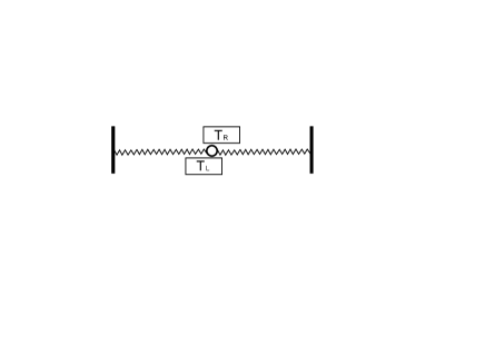
Figure 2: Single harmonic oscillator simultaneously coupled to two baths at different temperatures $T_{L}$ and $T_{R}$.

V.2 Two harmonic oscillators coupled to two baths

Two harmonic oscillators respectively coupled to two baths as shown in Fig. 3 is the special case of model system considered in Sec. II with $N=2$. In this case, the elastic matrix and the frictional matrix are assumed to be $\mathbf{K}=\left[\begin{array}[]{cc}k_{1}&\bar{k}\\ \bar{k}&k_{2}\end{array}\right]$ and $\bm{\Gamma}=\left[\begin{array}[]{cc}\gamma_{L}&0\\ 0&\gamma_{R}\end{array}\right]$.

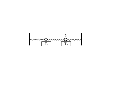
Figure 3: Two harmonic oscillators coupled to two baths at different temperatures $T_{L}$ and $T_{R}$.

Taking $\mathbf{E}_{L}=\left[\begin{array}[]{cc}1&0\\ 0&0\end{array}\right]$, from Eqs. (36)-(41), we can obtain the expressions of $\mathbf{B}_{L}$ and $\mathbf{G}_{L}$. Here we only write out their diagonal elements:

$$B_{L11}=G_{L11}=\frac{\bar{k}^{2}(\gamma_{L}+\gamma_{R})+\gamma_{R}\Omega}{\bar{k}^{2}(\gamma_{L}+\gamma_{R})^{2}+\gamma_{L}\gamma_{R}\Omega},$$ (47)

$$B_{L22}=G_{L22}=\frac{\bar{k}^{2}(\gamma_{L}+\gamma_{R})}{\bar{k}^{2}(\gamma_{L}+\gamma_{R})^{2}+\gamma_{L}\gamma_{R}\Omega},$$ (48)

where $\Omega\equiv\left(k_{1}-k_{2}\right)^{2}+\left(\gamma_{L}+\gamma_{R}\right)\left(k_{1}\gamma_{R}+k_{2}\gamma_{L}\right)$.

Similarly, taking $\mathbf{E}_{R}=\left[\begin{array}[]{cc}0&0\\ 0&1\end{array}\right]$, from Eqs. (36)-(41), we can obtain the expressions of $\mathbf{B}_{R}$ and $\mathbf{G}_{R}$. Here we only show their diagonal elements:

$$B_{R11}=G_{R11}=\frac{\bar{k}^{2}(\gamma_{L}+\gamma_{R})}{\bar{k}^{2}(\gamma_{L}+\gamma_{R})^{2}+\gamma_{L}\gamma_{R}\Omega},$$ (49)

$$B_{R22}=G_{R22}=\frac{\bar{k}^{2}(\gamma_{L}+\gamma_{R})+\gamma_{L}\Omega}{\bar{k}^{2}(\gamma_{L}+\gamma_{R})^{2}+\gamma_{L}\gamma_{R}\Omega}.$$ (50)

With these diagonal elements, we can calculate $C_{L}$ and $C_{R}$ by using Eqs. (42) and (43). The corresponding expressions are as follows:

$$C_{L}=\frac{2\bar{k}^{2}\gamma_{L}\left(\gamma_{L}+\gamma_{R}\right)+\gamma_{L}\gamma_{R}\Omega}{2\bar{k}^{2}\left(\gamma_{L}+\gamma_{R}\right)^{2}+2\gamma_{L}\gamma_{R}\Omega},$$ (51)

$$C_{R}=\frac{2\bar{k}^{2}\gamma_{R}\left(\gamma_{L}+\gamma_{R}\right)+\gamma_{L}\gamma_{R}\Omega}{2\bar{k}^{2}\left(\gamma_{L}+\gamma_{R}\right)^{2}+2\gamma_{L}\gamma_{R}\Omega}.$$ (52)

The corresponding effective temperature is

$$T_{e} = \frac{2\bar{k}^{2}\gamma_{L}\left(\gamma_{L}+\gamma_{R}\right)+\gamma_{L}\gamma_{R}\Omega}{2\bar{k}^{2}\left(\gamma_{L}+\gamma_{R}\right)^{2}+2\gamma_{L}\gamma_{R}\Omega}T_{L}$$ (53)

$$+ \frac{2\bar{k}^{2}\gamma_{R}\left(\gamma_{L}+\gamma_{R}\right)+\gamma_{L}\gamma_{R}\Omega}{2\bar{k}^{2}\left(\gamma_{L}+\gamma_{R}\right)^{2}+2\gamma_{L}\gamma_{R}\Omega}T_{R}.$$ (54)

In general, the weight factors $C_{L}$ and $C_{R}$ are unequal to each other. If $\gamma_{L}=\gamma_{R}$, the system is symmetrical coupling to both baths. In this situation, Eqs. (51) and (52) lead to $C_{L}=C_{R}=1/2$ and then the effective temperature $T_{e}=\bar{T}\equiv(T_{L}+T_{R})/2$, which is in good agreement with our intuition that the effective temperature of a harmonic chain equals to the mean temperature of two baths when the system simultaneously satisfies two symmetry conditions: (i) the interactions between oscillators in the chain are of left-right symmetry; (ii) two ends of the chain are symmetrically coupled to two baths. It is noted that the first condition holds automatically for a chain of two oscillators. Thus if and only if the second condition is satisfied, the effective temperature for a chain of two oscillators equals to the mean temperature of two baths.

V.3 Asymmetrical chain of three harmonic oscillators with two ends symmetrically coupled to two baths

Let us consider a chain of three harmonic oscillators with two ends coupled to two baths as shown in Fig. 4. We adopt the same values of elastic matrix and frictional matrix as those in Ref. [22]. For $N=3$, the elastic matrix is $\mathbf{K}=k_{0}\left[\begin{array}[]{ccc}2&-1&0\\ -1&3&-2\\ 0&-2&2\end{array}\right],$ where $k_{0}=m\omega^{2}$ is the reference elastic constant. For simplicity, we set $k_{0}$ to be unit in the following discussions. The off-diagonal elements of $\mathbf{K}$ are different from each other, which implies that interactions between harmonic oscillators are asymmetrical. The frictional matrix is $\bm{\Gamma}=\left[\begin{array}[]{lll}\gamma&0&0\\ 0&0&0\\ 0&0&\gamma\end{array}\right]$. Since two frictional constants are equal to each other, two ends of the chain are symmetrically coupled to two baths. We expect that the effective temperature should be different from the mean temperature of two baths since the first symmetry condition mentioned at the end of subsection V.2 is broken in this model.

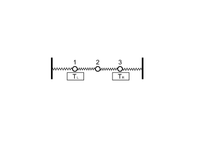
Figure 4: A chain of three harmonic oscillators with two ends coupled to two baths at different temperatures $T_{L}$ and $T_{R}$.

Taking $\mathbf{E}_{L}=\left[\begin{array}[]{ccc}1&0&0\\ 0&0&0\\ 0&0&0\end{array}\right]$, we can obtain the expressions of $\mathbf{B}_{L}$ and $\mathbf{G}_{L}$. Their diagonal elements are:

$$B_{L11}=G_{L11}=\frac{85+158\gamma^{2}+70\gamma^{4}}{5\gamma\left(25+38\gamma^{2}+14\gamma^{4}\right)},$$ (55)

$$B_{L22}=G_{L22}=\frac{1}{5\gamma},$$ (56)

$$B_{L33}=G_{L33}=\frac{40+32\gamma^{2}}{5\gamma\left(25+38\gamma^{2}+14\gamma^{4}\right)}.$$ (57)

Similarly, with the consideration of $\mathbf{E}_{R}=\left[\begin{array}[]{ccc}0&0&0\\ 0&0&0\\ 0&0&1\end{array}\right]$, we can derive the expressions of $\mathbf{B}_{R}$ and $\mathbf{G}_{R}$. Their diagonal elements are:

$$B_{R11}=G_{R11}=\frac{40+32\gamma^{2}}{5\gamma\left(25+38\gamma^{2}+14\gamma^{4}\right)},$$ (58)

$$B_{R22}=G_{R22}=\frac{4}{5\gamma},$$ (59)

$$B_{R33}=G_{R33}=\frac{85+158\gamma^{2}+74\gamma^{4}}{5\gamma\left(25+38\gamma^{2}+14\gamma^{4}\right)}.$$ (60)

Substituting these diagonal elements into Eqs. (42) and (43), we have

$$C_{L}=\frac{2}{5},~{}\mathrm{and}~{}C_{R}=\frac{3}{5}.$$ (61)

Correspondingly, the effective temperature is

$$T_{e}=\frac{2T_{L}+3T_{R}}{5}.$$ (62)

Just as we expect, the effective temperature is indeed different from the mean temperature $\bar{T}\equiv(T_{L}+T_{R})/2$ since the first symmetry condition mentioned at the end of subsection V.2 is broken in this model.

With the consideration of Eq. (27), we derive the internal energy $\mathcal{E}=3T_{e}=3(2T_{L}+3T_{R})/5$. This result can be rewritten as

$$\mathcal{E}=3\bar{T}-\frac{3\Delta T}{10},$$ (63)

which is identical to Eq. (95) obtained by Wu and Wang in Ref. [22]. In other words, the internal energy can be expressed in a concise form with the weighted average temperature, while still leads to the correct result.

V.4 Symmetrical chain of three harmonic oscillators with two ends asymmetrically coupled to two baths

Let us consider the same setup as in the above subsection but with different values of elastic matrix and frictional matrix. Take the elastic matrix $\mathbf{K}=\left[\begin{array}[]{ccc}2&-1&0\\ -1&3&-1\\ 0&-1&2\end{array}\right].$ The off-diagonal elements of $\mathbf{K}$ are equal to each other, which implies that the chain of three harmonic oscillators is symmetrical. Take the frictional matrix $\bm{\Gamma}=\gamma_{0}\left[\begin{array}[]{lll}1&0&0\\ 0&0&0\\ 0&0&\bar{\gamma}\end{array}\right]$ where $\gamma_{0}$ is the reference frictional constant which is set to be unit in the following discussions. Two ends of the chain are asymmetrically coupled to two baths if $\bar{\gamma}\neq 1$. In this situation, we expect that the effective temperature should be different from the mean temperature of two baths since the second symmetry condition mentioned at the end of subsection V.2 is broken in this model.

Taking $\mathbf{E}_{L}=\left[\begin{array}[]{ccc}1&0&0\\ 0&0&0\\ 0&0&0\end{array}\right]$, we can obtain the expressions of $\mathbf{B}_{L}$ and $\mathbf{G}_{L}$. Their diagonal elements are:

$$B_{L11}=G_{L11}=\frac{1+5\bar{\gamma}+8\bar{\gamma}^{2}+5\bar{\gamma}^{3}}{1+6\bar{\gamma}+10\bar{\gamma}^{2}+5\bar{\gamma}^{3}},$$ (64)

$$B_{L22}=G_{L22}=\frac{1+3\bar{\gamma}+2\bar{\gamma}^{2}+5\bar{\gamma}^{3}}{1+6\bar{\gamma}+10\bar{\gamma}^{2}+5\bar{\gamma}^{3}},$$ (65)

$$B_{L33}=G_{L33}=\frac{1+2\bar{\gamma}}{1+6\bar{\gamma}+10\bar{\gamma}^{2}+5\bar{\gamma}^{3}}.$$ (66)

Similarly, with the consideration of $\mathbf{E}_{R}=\left[\begin{array}[]{ccc}0&0&0\\ 0&0&0\\ 0&0&1\end{array}\right]$, we can derive the expressions of $\mathbf{B}_{R}$ and $\mathbf{G}_{R}$. Their diagonal elements are:

$$B_{R11}=G_{R11}=\frac{1+2\bar{\gamma}}{1+6\bar{\gamma}+10\bar{\gamma}^{2}+5\bar{\gamma}^{3}},$$ (67)

$$B_{R22}=G_{R22}=\frac{3+8\bar{\gamma}}{1+6\bar{\gamma}+10\bar{\gamma}^{2}+5\bar{\gamma}^{3}},$$ (68)

$$B_{R33}=G_{R33}=\frac{4+10\bar{\gamma}+5\bar{\gamma}^{2}}{1+6\bar{\gamma}+10\bar{\gamma}^{2}+5\bar{\gamma}^{3}}.$$ (69)

Substituting these diagonal elements into Eqs. (42) and (43), we have

$$C_{L}=\frac{3+10\bar{\gamma}+10\bar{\gamma}^{2}+10\bar{\gamma}^{3}}{3+18\bar{\gamma}+30\bar{\gamma}^{2}+15\bar{\gamma}^{3}},$$ (70)

and

$$C_{R}=\frac{8\bar{\gamma}+20\bar{\gamma}^{2}+5\bar{\gamma}^{3}}{3+18\bar{\gamma}+30\bar{\gamma}^{2}+15\bar{\gamma}^{3}}.$$ (71)

Correspondingly, the effective temperature is

$$T_{e} = \frac{3+10\bar{\gamma}+10\bar{\gamma}^{2}+10\bar{\gamma}^{3}}{3+18\bar{\gamma}+30\bar{\gamma}^{2}+15\bar{\gamma}^{3}}T_{L}$$ (72)

$$+ \frac{8\bar{\gamma}+20\bar{\gamma}^{2}+5\bar{\gamma}^{3}}{3+18\bar{\gamma}+30\bar{\gamma}^{2}+15\bar{\gamma}^{3}}T_{R}.$$ (73)

In general, as we expect, the weight factors $C_{L}\neq C_{R}$ if $\bar{\gamma}\neq 1$. In particular, the system is symmetrically coupled to both baths if $\bar{\gamma}=1$. In this situation, Eqs. (70) and (71) lead to $C_{L}=C_{R}=1/2$ and then the effective temperature $T_{e}=\bar{T}\equiv(T_{L}+T_{R})/2$, which is in good agreement with our intuition since the system simultaneously satisfies two symmetry conditions mentioned at the end of subsection V.2.

VI Conclusion and discussion

We have investigated the effective temperature at steady state of a harmonic chain coupled to two thermal baths at different temperatures. The key ansatz is that the revised covariance matrix may be decomposed into the diagonal matrix and traceless residual matrix [see Eqs. (10) and (11)] . We suggest taking the weighted average temperature [Eq. (17)] as the effective temperature of the system. The weight factors [Eq. (18)] are related to the coupling constants between the system and two baths as well as the asymmetry of interactions between oscillators. The residual matrix [ Eq. (19)] depends linearly on the temperature difference between two thermal baths. The advantage of weighted average temperature lies in revisiting the thermodynamics of nonequilbrium steady states. The fundamental thermodynamic relations in nonequilbrium steady states such as internal energy [Eq. (27)], entropy [Eq. (28)], and free energy [Eq. (29)] possess similar concise forms as those in equilibrium thermodynamics. The minor difference is to replace the temperature in equilibrium with the weighted average temperature in steady states. The nonequilbrium character manifests in the heat transfer and entropy production. The heat transfer rate [Eq. (32)] is proportional to the temperature difference between two baths, while the entropy production rate [Eq. (34)] is proportional to the quadratic term of temperature difference. Finally, we also illustrate the procedure to calculate the effective temperatures via four examples.

Before ending this paper, we address two issues which are not touched in the main text. (i) The model that we employed is of linearity. If the equations of motion contain nonlinear forces, the steady-state distribution cannot directly be expressed with the covariance matrix. Therefore, our proposed definition of effective temperature based on the decomposition of covariance matrix does not hold for nonlinear systems. It is still a challenge to extend the present idea to the situations including nonlinear forces. (ii) A typical proposal in previous literature is to define effective temperature using the violation of fluctuation-dissipation theorem [3, 4, 5, 6, 7]. In the above discussions, we propose to define the effective temperature via the weighted average temperature. But it is unclear to make a connection between two kinds of definitions. We will further investigate these issues in the future work.

References

- [1] M. J. Klein, Thermodynamics in Einstein's thought, Science 157, 509 (1967).
- [2] J. A. McLennan, Introduction to Non-equilibrium Statistical Mechanics (Prentice Hall, New Jersey, 1989)
- [3] J Casas-Vázquez1 and D Jou, Temperature in non-equilibrium states: a review of open problems and current proposals, Rep. Prog. Phys. 66, 1937 (2003).
- [4] L. F. Cugliandolo, J. Kurchan, and L. Peliti, Energy flow, partial equilibration, and effective temperatures in systems with slow dynamics, Phys. Rev. E 55, 3898 (1997).
- [5] L. F. Cugliandolo, The effective temperature, J. Phys. A: Math. Theor. 44, 483001 (2011).
- [6] A. Puglisi, A. Sarracino, and A. Vulpiani, Temperature in and out of equilibrium: a review of concepts, tools and attempts, Phys. Rep. 709-710, 1 (2017).
- [7] D. Zhang, X. Zheng, and M. Di Ventra, Local temperatures out of equilibrium, Phys. Rep. 830, 1 (2019).
- [8] S. Fielding and P. Sollich, Observable dependence of fluctuation-dissipation relations and effective temperatures, Phys. Rev. Lett. 88, 050603 (2002).
- [9] E. Ben-Isaac, Y. Park, G. Popescu, F. L. H. Brown, N. S. Gov, and Y. Shokef, Effective temperature of red-blood-cell membrane fluctuations, Phys. Rev. Lett. 106, 238103 (2011).
- [10] S. Jabbari-Farouji, D. Mizuno, D. Derks, G. H. Wegdam, F. C. MacKintosh, C. F. Schmidt, and D. Bonn, Effective temperatures from the fluctuation-dissipation measurements in soft glassy material, EPL 84, 20006 (2008).
- [11] K. Hayashi and S. Sasa, Effective temperature in nonequilibrium steady states of Langevin systems with a tilted periodic potential, Phys. Rev. E. 69, 066119 (2004).
- [12] C. S. O'Hern, A. J. Liu, and S. R. Nagel, Effective temperatures in driven systems: static versus time-dependent relations, Phys. Rev. Lett. 93, 165702 (2004).
- [13] T. K. Haxton and A. J. Liu, Activated dynamics and effective temperature in a steady state sheared glass, Phys. Rev. Lett. 99, 195701 (2007).
- [14] N. Xu and C. S. O'Hern, Effective temperature in athermal systems sheared at fixed normal load, Phys. Rev. Lett. 94, 055701 (2005).
- [15] A. R. Abate and D. J. Durian, effective temperatures and activated dynamics for a two-dimensional air-driven granular system on two approaches to jamming, Phys. Rev. Lett. 101, 245701 (2008).
- [16] S. Joubaud, B. Percier, A. Petrosyan, and S. Ciliberto, Aging and effective temperatures near a critical point, Phys. Rev. Lett. 102, 130601 (2009).
- [17] A. Caso, L. Arrachea, and G. S. Lozano, Local and effective temperatures of quantum driven systems, Phys. Rev. B 81, 041301(R) (2010).
- [18] L. Joly, S. Merabia, and J.-L. Barrat, Effective temperatures of a heated Brownian particle, EPL 94, 50007 (2011).
- [19] B. Lander, U. Seifert, and T. Speck, Effective confinement as origin of the equivalence of kinetic temperature and fluctuation-dissipation ratio in a dense shear-driven suspension, Phys. Rev. E 85, 021103 (2012).
- [20] M. Zhang and G. Szamel, Effective temperatures of a driven, strongly anisotropic Brownian system, Phys. Rev. E 83, 061407 (2011).
- [21] J. M. R. Parrondo and P. Español, Criticism of Feynman's analysis of the ratchet as an engine, Am. J. Phys. 64, 1125 (1996).
- [22] W. Wu and J. Wang, Nonequilibrium equation of state for open Hamiltonian systems maintained in nonequilibrium steady states, J. Phys. Chem. B 126, 7883 (2022).
- [23] H. Ness, Nonequilibrium density matrix in quantum open systems: generalization for simultaneous heat and charge steady-state transport, Phys. Rev. E 90, 062119 (2014).
- [24] C. Van den Broeck, E. Kestemont, and M. Malek Mansour, Heat conductivity by a shared piston, Europhys. Lett. 56, 771 (2001).
- [25] Y. Murashita and M. Esposito, Overdamped stochastic thermodynamics with multiple reservoirs, Phys. Rev. E. 94, 062148 (2016).
- [26] J. S. Lee and H. Park, Additivity of multiple heat reservoirs in the Langevin equation, Phys. Rev. E. 97, 062135 (2018).
- [27] C. Y. Hsieh, J. Liu, C. Duan, and J. Cao, A nonequilibrium variational polaron theory to study quantum heat transport, J. Phys. Chem. C 123, 17196 (2019).
- [28] S. Sheng and Z. C. Tu, Weighted reciprocal of temperature, weighted thermal flux, and their applications in finite-time thermodynamics, Phys. Rev. E. 89, 012129 (2014).
- [29] C. Gardiner, Handbook of Stochastic Methods (Springer-Verlag, Berlin, 1997).
- [30] H. Risken, The Fokker-Planck Equation (Springer-Verlag: Berlin, 1996).