Rapid Optimization of Superposition Codes for Multi-Hop NOMA MANETs via Deep Unfolding
Abstract
Various communication technologies are expected to utilize mobile ad hoc networks. By combining MANETs with non-orthogonal multiple access (NOMA) communications, one can support scalable, spectrally efficient, and flexible network topologies. To achieve these benefits of NOMA MANETs, one should determine the transmission protocol, particularly the superposition code. However, the latter involves lengthy optimization that has to be repeated when the topology changes. In this work, we propose an algorithm for rapidly optimizing superposition codes in multi-hop NOMA MANETs. To achieve reliable tunning with few iterations, we adopt the emerging deep unfolding methodology, leveraging data to boost reliable settings. Our superposition coding optimization algorithm utilizes a small number of projected gradient steps while learning its per-user hyperparameters to maximize the minimal rate over past channels in an unsupervised manner. The learned optimizer is designed for both settings with full channel state information, as well as when the channel coefficients are to be estimated from pilots. We show that the combination of principled optimization and machine learning yields a scalable optimizer, that once trained, can be applied to different topologies. We cope with the non-convex nature of the optimization problem by applying parallel-learned optimization with different starting points as a form of ensemble learning. Our numerical results demonstrate that the proposed method enables the rapid setting of high-rate superposition codes for various channels.
I Introduction
A broad range of communication technologies, ranging from industrial systems [2] to drone swarms [3] and tactical networks [4], are subject to strict demands in terms of connectivity, robustness, mobility, and security. An emerging paradigm shift aimed at meeting these requirements is to deviate from the uplink/downlink star topology operation of conventional wireless communications, e.g., cellular networks. Among the leading approaches for realizing dynamic and flexible networks is the MANET technology [5], where communication links are established during operation, possibly on demand and over multi-hop routes. Forming multi-hop communication topologies on demand allows mobile communicating entities to collaborate in communication and decision-making [6].
One of the core challenges in multi-user communications, which grows more prominent in MANETs compared to traditional topologies, is the presence and treatment of cross interference. Such interference naturally arises from the fact that multiple users share the same temporal and spectral channel resources. Arguably the most common strategy in conventional wireless communications to deal with cross-interference is to mitigate it, i.e., to boost orthogonality among the communicating entities. This can be achieved via the division of the spectral and temporal resources, or alternatively via media access protocols designed to prevent collisions. While orthgonalizing multi-user communications facilitates system design, it comes at the cost of throughput degradation due to its sub-optimal usage of the channel resources [7]. Consequently, recent years have witnessed a growing interest in transiting from orthogonality-based communications to NOMA solutions [8, 9]. NOMA allows users to simultaneously share the channel resources for supporting heterogeneous end-devices. However, non-orthogonal multi-user communications inevitably impose interference.
Various receive methods have been proposed for enabling reliable communications in the presence of interference [10]. A widely adopted receiver algorithm for non-orthogonal broadcast channels is successive interference cancellation (SIC), which is based on successively decoding a set of superimposed messages that are transmitted to different users over a shared channel. The gains of SIC are also indicated in its ability to approach the achievable rate region of such channels when combined with superposition coding [8, 9, 11], whilst its complexity only grows linearly with the number of users. Similar approaches for handling interference via superposition coding and interference cancellation at the receiver were also proposed for multiple access channels [12, 13].
The theoretical benefits of NOMA are widely studied in the context of conventional uplink/downlink wireless communications, based on BC/MAC modeling, respectively. While these studies consider star topologies, recent works have identified that these gains can also be harnessed in multi-hop topologies [14], and thus potentially also in MANETs. In order to harness these gains of NOMA, one should determine the superposition code utilized by all communicating entities based on the current channel realization. In MANETs, which are inherently designed for dynamic and mobile settings, the channel realizations, and even the network topology, often vary rapidly. Thus, superposition code setting has to be repeated frequently based on possibly noisy channel estimates. Nonetheless, this procedure involves lengthy optimization even for conventional topologies, with recent studies proposing iterative methods [15] and the usage of machine learning architectures [16, 17]. However, the setting of superposition codes is notably more complicated in MANETs, particularly when using noisy channel estimates. This motivates the design of efficient optimization techniques for rapidly and reliably configuring NOMA MANETs.
In this work, we propose an algorithm that rapidly optimizes superposition code for multi-hop NOMA MANETs. Our proposed method, based on unfolding projected gradient descent (PGD) optimization, is coined Unfolded PGDNet. Unfolded PGDNet tunes the superposition code for a given MANET based on noisy limited pilots, using estimated channel state information (CSI) as indicative features. We derive our method by formulating the superposition code design as a non-convex constrained optimization problem aiming at maximizing the minimal rate in the network. We then leverage emerging learn-to-optimize methodologies [18, 19], and particularly deep unfolding [20, 21], to learn from data how to enable projected gradient steps to rapidly recover a suitable configuration and cope with noisy channel estimates.
As the minimal rate objective of the superposition coding optimization is non-convex, we tackle it by proposing an ensemble method [22]. In particular, we apply in parallel multiple instances of the learned optimizer with different initial settings; the algorithm then identifies multiple candidate solutions and selects the one with the best minimal rate. While we train Unfolded PGDNet for a given topology, we show that its interpretable operation renders it transferable to multiple different topologies. Accordingly, Unfolded PGDNet facilitates rapid adaptation of superposition codes in dynamic MANETs, coping not only with variations in the channel realizations for a given topology, but also with variations in the topology itself. Our numerical results demonstrate that Unfolded PGDNet rapidly produces solid superposition code configurations, reducing the latency compared with conventional optimization by factors varying from to over , as well as consistently outperforming competing data-driven techniques based on graph neural networks [23].
The rest of this work is organized as follows: Section II describes the system model; the proposed learn-to-optimize algorithm for configuring NOMA MANETs is detailed in Section III, and is numerically evaluated in Section IV. Finally, Section V provides concluding remarks.
Throughout the paper, we use boldface lower-case letters for vectors, e.g., ; the th element of is written as . Matrices are denoted with boldface upper-case letters, e.g., ; is its th element, while is its th row. Calligraphic letters, such as , are used for sets, while denotes the real numbers. The norm, transpose, and Hermitian transpose are written as , , and , respectively.
II System Model
In this section, we formulate the system model for multi-hop NOMA MANETs. We commence with presenting the communication system in Subsection II-A, and how CSI is acquired in Subsection II-B. Based on these, we formulate the superposition coding optimization problem in Subsection II-C, which constitutes the starting point for our derivation of Unfolded PGDNet in the sequel.
II-A Communication System Model
We consider a block-fading multi-hop scalar MANET with a single transmitter and multiple receiver nodes (end-users). There are no direct links between the transmitter and the receivers, and communication is achieved only via intermediate relays spreading over hops. The channels and the MANET topology are block-wise time-varying, representing the ad-hoc nature of such networks. In each coherence duration of index , the transmitter wishes to communicate with end-users, while the th hop involves relays for each , with , as the th hop reaches the end-users. An example topology is illustrated in Fig. 1.
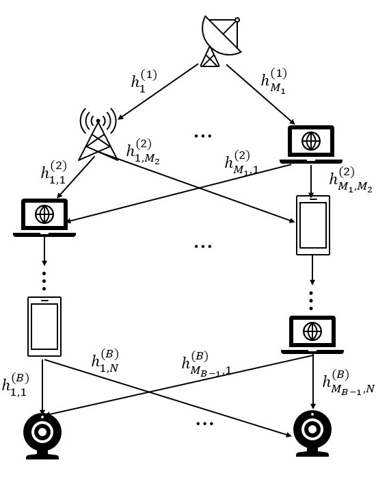
The communicating devices employ power domain NOMA [9]. Accordingly, letting denote the signal intended for the th end-user at the th coherence duration, , the transmitter generates a linear combination of via superposition coding weighted by the non-negative power coefficients . Let denote the channel coefficient between the transmitter and the th relay of the first hop, which is constant during the coherence duration by the block-fading model [24, Ch. 3]. The signal received by the th relay of the first hop is given by
| (1) |
for each . In (1), is additive white Gaussian noise (AWGN) with variance for each hop .
The relays operate in a decode-and-forward manner [7, Ch. 16], aiming to recover from their corresponding channel output (1). Then, are relayed to the next hop, with each relay employing a dedicated superposition code. We use to denote the power coefficients of the th relay at the th hop. Let be the channel from the th relay to the th receiving node at the th hop over the th coherence period. The signal received at this receiving node is obtained as
| (2) |
for each . For clarity, we summarize the variables defined above in Table I.
Decoding at both the relays and the end-users is carried out using SIC, whose combination with superposition coding is known to approach the capacity region of single-hop NOMA systems [9]. SIC operates iteratively: first the signal with the highest signal-to-interference-and-noise ratio (SINR) is decoded, while treating all the other signals as noise. Then, it is subtracted from the superimposed message and the signal with the second largest SINR is recovered in the same fashion. This procedure is carried out over all messages at the relays (which decode all messages for decode-and-forward), while the th end-user terminates SIC when decoding .
| Symbol | Definition |
|---|---|
| i.i.d AWGN noise at th receiver, th hop | |
| transmitter - th relay at first hop channel | |
| th relay - th receiver at th hop channel | |
| signal intended for th end-user | |
| transmit power allocate to th signal at first hop | |
| th hop th relay power allocate to th signal |
II-B Channel State Information
The block-fading nature of the considered channel model indicates that the communicating entities are likely not to have CSI, i.e., prior knowledge of the channel coefficients. Hence, they would be required to estimate it from periodic pilots. To that aim, we assume that each coherence duration is commenced with a transmission of pilots, whose quantity is always larger than the number of transmitters in each hop, i.e., . Let denote the pilots vector sent by the th transmitter at the th hop. Following conventional pilot modeling, e.g., [25, 26], it is assumed that the pilots are orthonormal, i.e., that if and zero otherwise.
A candidate approach to utilize the pilots to estimate the channel uses the linear minimum mean-squared error (LMMSE) estimator. To formulate this estimator, let be the vector representing the channel outputs corresponding to the pilots obtained at the th receiving node of the th hop during the th block. Assuming that the channel coefficients are all zero-mean and with variance , the LMMSE estimate of the channel is [27, Ch. 8]
| (3) |
Similarly, at subsequent hops, is estimated as
| (4) |
II-C Problem Formulation
II-C1 Achievable Rates
The communication model for the considered NOMA MANET is formulated in Subsection II-A for an arbitrary superposition code, dictated by the power coefficients and . However, the exact setting of the code coefficients notably affects the achievable communication rate in the MANET. In particular, by (1) the th message is recoverable by the th relay of the first hop (with arbitrarily small error probability) if it is coded with a rate (in bits per channel use), not larger than [24, Ch. 6]
| (5) |
where we defined
The message also has to be recoverable by each relay as well as its corresponding end-user. In particular, the th message is decoded by all relays, as well as by the th end-user, by recovering all messages preceding it via SIC. By (2), the th message can be recovered by the the receiving node at the th hop when its rate is not larger than
| (6) |
for all hop . In (6), we defined:
| (7) |
and
II-C2 Superposition Code Optimization
The rate expressions in (5) and (6) depend on the superposition coding coefficients, written henceforth as the matrix , where . The matrix is comprised of sub-matrices , and a vector . The entries of the sub-matrices are given by for where , while . To create , we stack
| (8) |
Using these notations combined with (6) and (5), and by stacking the MANET channel coefficients as the vector , the rate supported for the th message is given by
| (9) |
In (9), the first minimization term corresponds to the fact that each end-user does not have to recover all messages, only those preceding and including its own in the superposition code. However, each relay decodes all messages (as encapsulated in the second term), and thus the coding rate must be set such that the message can be reliably decoded by all these nodes.
We aim to set the superposition coding coefficients to maximize the minimal rate, i.e., the throughput one can guarantee for all end-users, being a key performance measure in MANETs. Without loss of generality, we assume a unit power constraint on each of the transmitting devices, i.e., , where is defined as
| (10) |
Accordingly, our goal is to map the received pilots into a superposition code, i.e., knowledge of
| (11) |
and , into the coefficients matrix
| (12) |
II-C3 Challenges
The superposition code design problem formulated in (12) gives rise to several challenges. These challenges that are associated with the statement of the problem in (12), as well as with the dynamic nature of MANETs and its block-faded model, as summarized below:
-
C1
The optimization problem is non-convex, thus recovering the optimal may be infeasible. Moreover, even finding a good setting of (in the sense of increasing the minimal rate) is likely to involve lengthy iterative solvers.
-
C2
The superposition code has to be set anew each time the channel coefficients changes. Thus, the design has to be carried out rapidly, e.g., within a small and fixed number of iterative steps.
-
C3
The channel realizations, which are necessary for rate calculation, are not available. Instead, they must estimated from noisy pilots, resulting in inaccurate CSI.
-
C4
One of the main properties of MANETs is their dynamic topology, which changes over time. A solver to (12) must be flexible thus to different topologies.
To facilitate tackling (12) while coping with C1-C4, we assume access to a set of past channel realizations. This data is available offline, i.e., when designing the solver, and can be obtained from past measurements. The resulting data set is denoted by
| (13) |
with denoting the stacking of the MANET channel realizations at block , while stacks the noise variances. The availability of data indicates the possibility of leveraging machine learning tools, combined with principled optimization to cope with C1-C4, as proposed in the following section.
III Unfolded Superposition Coding Optimization
This section presents our proposed data-aided optimizer for rapid superposition code design. We gradually derive our method based on the following steps:
-
•
We first formulate the PGD steps for tackling (12) in Subsection III-A. PGD is suitable for convex problems [28, Ch. 9]; it assumes CSI; and it typically requires many iterations to converge. Accordingly, it is not tailored to tackle C1-C4 on its own. Instead, it is used as our basis optimizer due to its simplicity and interpretability.
-
•
Then, in Subsection III-B we convert PGD into PGDNet, which is designed to tackle C1-C2 (without dealing with C3-C4 yet). We assume full CSI and a static MANET topology. For such setting, we leverage data to optimize the PGD optimizer, i.e., we learn-to-optimize rapidly [29], via deep unfolding methodology [20, 21] (thus tackling C2), and extend it to cope with C1 using an ensemble of Unfolded PGDNet model.
- •
- •
We next elaborate on these steps, followed by a dedicated in discussion in Subsection III-E.
III-A Projected Gradient Descent for NOMA MANETs
Problem (12) represents constrained maximization with optimization variables. While the problem is non-convex, one can identify a plausible setting for the superposition code parameters by applying iterative PGD steps starting from some suitable initialization . The resulting iterative procedure at iteration index is given by
| (14) |
where is the step-size, and denotes the projection operator onto . As the projection operator onto the simplex (10) typically involves additional iterative procedures [30], we approximate it using the following operator (which guarantees that the projection of any matrix with at least one positive entry per column indeed lies in by (10)), written as , with
| (15) |
In (15), is the positive part operator, i.e., , applied element-wise.
To implement PGD, the gradients of the objective function are required. These are stated in the following lemma.
Lemma 1.
For a given , let , , and , be the indices holding and . Then, for each and it holds that
| (16a) | ||||
| (16b) | ||||
where the gradients of are given in (17).
| (17a) | ||||
| (17b) | ||||
Proof:
See Appendix -A. ∎
The resulting optimization method with iterations is summarized as Algorithm 1 (where the time index is omitted). Note that the computation requires knowledge of the CSI, denoted by the vector which includes all channel realizations in the MANET. Moreover, PGD is inherently designed for convex objectives, and typically requires to be large to achieve convergence with a fixed step-size [31]. While this implies that the PGD optimizer in Algorithm 1 is on its own not suitable for the problem at hand, we use it as a form of inductive bias to obtain a data-aided optimizer capable of coping with C1-C4 in the following subsections.
III-B Unfolded PGDNet
Let us first assume a static topology of the MANET and access to full CSI, thus ignoring C3-C4 for the time being. Accordingly, in this subsection (as well as in Subsection III-C) we omit the block index for brevity.
Algorithm 1 optimizes the power allocation for a given MANET realization. However, its convergence speed highly depends on the hyperparameters, i.e., the step-sizes , and the resulting rate can be notably affected by the initial guess due to the non-convexity. We thus propose a data-aided implementation of PGD, termed Unfolded PGDNet. We derive our method based on the following steps: We first tackle C2 converting PGD into a fixed-latency discriminative trainable architecture [32] via deep unfolding methodology [21], and propose dedicated training algorithm; Then, we extend it into an ensemble of multiple parallel models that converge to different local optima to cope with C1.
III-B1 PGDNet Architecture
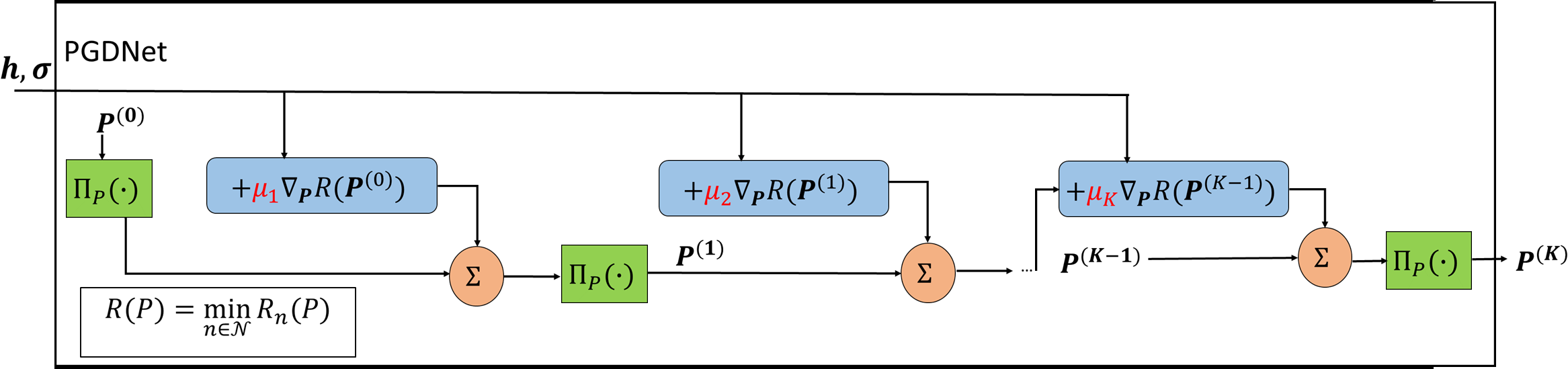
We propose to leverage data to learn-to-optimize based on deep unfolding [21]. This methodology converts iterative optimizers with a predetermined number of iterations into machine learning models. The proposed Unfolded PGDNet applies PGD (Algorithm 1) with a predefined (and small) number of iterations K. By doing that, we guarantee an a-priori known, and considerably low, run-time. While the accuracy of first-order optimizers such as PGD is usually invariant of hyperparameters setting when allowed to run until convergence (as long as the step-sizes are sufficiently small) [28], its performance is largely affected by these settings when the number of iterations is fixed.
In Unfolded PGDNet, we treat the hyperparameters of the iterative optimizer, i.e., , as the trainable parameters of a machine learning model. The resulting architecture can be viewed as a form of a deep neural network (DNN) with layers: Each layer of index implements a single PGD iteration, and has a single trainable parameter, which is the step-size . The resulting architecture is illustrated in Fig. 2. As in Algorithm 1, we denote its operation for CSI with hyperparameters and initial guess as .
III-B2 Training PGDNet
The training procedure aims to set the hyperparameters to make PGDNet maximize the minimal rate for the channel available in the data set in (13). As in [29], we also exploit the interpretability of the trainable architecture to facilitate and regularize the training procedure. Specifically, we account for the fact that the features exchanged between layers correspond to superposition coding coefficients, i.e., for the th layer, and encourage the model to learn gradually improved settings.
To formulate the resulting learning objective, we write as the output of the th iteration of PGDNet, i.e., . We train PGDNet by setting the loss function to be
| (18) |
where the logarithmic weights are used to have a growing contribution to the overall loss of the more advanced learned iterations [33]. Note that (18) enables unsupervised learning, i.e., there is no need to provide ‘ground truth‘ power allocation. This stems from the task being an optimization problem, for which one can evaluate each setting of the optimization variables.
The learn-to-optimize method, summarized as Algorithm 2, uses data to tune based on (18). We initialize before the training process with a fixed step-size with which PGD converges (given sufficient iterations). Then, we exploit the differentiability of the gradients in (16) and the projection operator in (15) to tune via conventional deep learning tools (where in Algorithm 2 we employ mini-batch stochastic gradient descent for learning). We modify the initial guess during training to have the learned hyperparameters be suitable for different starting points. At the end of the training process, the learned vector is used as a hyperparameter for rapid finding of the best power allocation for a given channel via iterations of Algorithm 1.
III-B3 PGDNet Ensemble
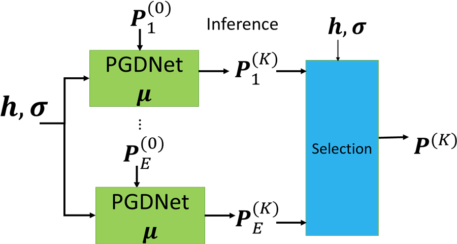
Unfolded PGDNet uses data to make PGD operate most efficiently within iterations (where is small). However, by C1 it is still expected to converge to a power allocation in the proximity of the initial guess , which is not necessarily the most suitable one. Nonetheless, by setting to be relatively small, one can apply Unfolded PGDNet times, each time with a different (thus accounting for C1), while still inferring sufficiently fast to cope with C2.
The resulting power allocation procedure thus utilizes an ensemble model [22] comprised of a parallel application of Unfolded PGDNet algorithms. Specifically, we train a single Unfolded PGDNet model, and learn the hyperparameters . Then, in runtime, given a channel realization , we apply Unfolded PGDNet with these hyperparameters , using different initial guesses denoted , as illustrated in Fig. 3(b). To select the superposition code, we leverage the fact that we can evaluate each suggested setting using the optimization objective in (12), and select the power allocation that gives the maximal min-rate among all the iterations of the ensemble models, i.e.,
| (19) |
III-C Learned Optimization from Noisy Pilots
Unfolded PGDNet detailed in the previous Subsection leverages data to enable PGD optimization of superposition codes while coping with C1-C2. However, it still requires the CSI to be provided to compute the optimization objective, as in the conventional PGD, while in our setting one has access only to noisy pilots by C3. To tackle this, we next extend Unfolded PGDNet to optimize from noisy pilots by leveraging LMMSE CSI estimates as input features.
III-C1 Inference
To carry out inference, i.e., set a superposition code, using Unfolded PGDNet, we use the LMMSE estimator formulated in Subsection II-B to translate the noisy pilots in (11) into noisy CSI features. Then, Unfolded PGDNet is applied as if these features represent the full CSI. The resulting inference procedure is summarized as Algorithm 3.
III-C2 Training
The inference procedure in Algorithm 3 applies PGDNet while treating the noisy CSI estimates as the real CSI. While this can in general lead to performance degradation, we train PGDNet to produce learned hyperparameters that result in optimized rates concerning the true CSI available in the data (13).
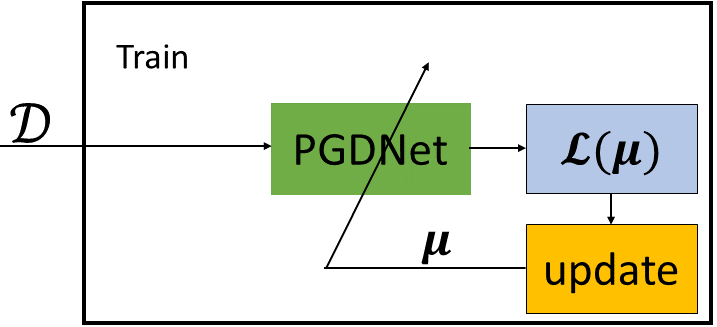
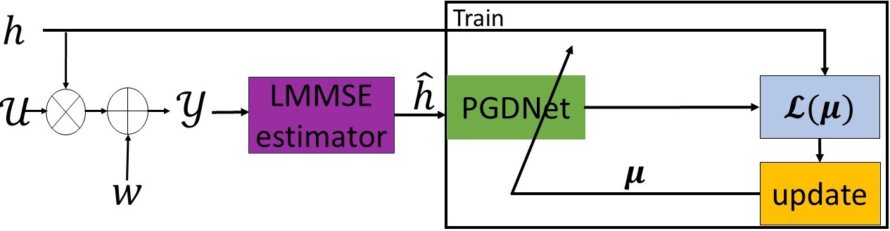
Consequently, the training procedure is based on Algorithm 2, with the core exception that the input is the LMMSE features, i.e., noisy CSI estimates, while the loss function in (18) is computed with the true CSI. Specifically, to compute the loss in Step 2 of Algorithm 2, we first use the observed channels in to simulate random channel observations via (1)-(2), from which the LMMSE estimate is computed via (3)-(4). Then, the loss gradients are taken not based on (18), but rather from
| (20) |
Namely, Unfolded PGDNet is applied to the batch of estimated CSI realizations, while the loss is computed using the true CSI. The procedure is illustrated in Fig. 4.
III-D Coping with Block-Fading Topologies
Our design of Unfolded PGDNet so far considers a given topology. However, as noted in C4, a key feature of MANETs is their dynamic nature, i.e., some links may be removed from the network and other devices may join the network after its setup, both ending up changing the topology. Additionally, even if the topology remains the same as we started with, due to the block-fading communication model, some links can be changed over time. While our design so far does not explicitly deal with these temporal variations, we advocate that its interpretable architecture, i.e., the fact that what is learned are hyperparameters of PGD optimization, enable it to cope with C4.
In particular, we note that conventional PGD in Algorithm 1 can be applied to different topologies. Moreover, its hyperparameters , which are learned and optimized from data via Algorithm 2, are invariant of the MANET topology. Consequently, PGDNet trained on a given topology is in fact transferable to alternative topologies, as we numerically demonstrate in Section IV. This allows a set of learned hyperparameters learned from past channel realizations via Algorithm 2 with the loss in (20) to be used by PGDNet inference in Algorithm 3 for block-fading MANETs.
III-E Discussion
Unfolded PGDNet is designed to produce superposition codes for a given NOMA MANET while coping with the non-convexity of the problem (C1), the need to design rapidly (C2), and the noisy and dynamic nature of MANETs (C3-C4). The former is tackled by employing an ensemble of convex optimizers and selecting the best candidate setting computed; the rapid operation of each optimizer is achieved by using data to optimize the optimizer via deep unfolding; and coping with dynamic settings follows from a dedicated learning procedure combined with the flexibility of its hybrid model-based/data-driven design. While classic approaches to improve convergence in terms of the number of iterations, e.g., line search [28, Ch. 9], come at the cost of increased latency due to additional processing carried out at each iteration, our unfolded method does not induce any excessive latency during inference compared to conventional PGD with fixed pre-determined step-sizes. As opposed to the application of machine learning architectures based on conventional DNNs, our data-aided algorithm is highly flexible to variations in the MANET topology. This makes our approach highly suitable for facilitating the rapid tuning of superposition codes.
The formulation of Unfolded PGDNet is invariant of the initial guesses . In our numerical study reported in Section IV we use equal power allocation for and randomize the remaining guesses uniformly over . This setting was empirically shown to be beneficial in terms of rapidly finding high min-rate superposition codes. Nonetheless, one can explore different settings of the initial guesses, which we leave for future investigation. Moreover, our derivation copes with noisy CSI by using LMMSE features, which require knowledge of the channel variance . One can replace these with a learned feature extractor which does not require such knowledge and can be possibly trained jointly with PGDNet. Finally, we note that we consider a centralized setting of the superposition code, i.e., all the superposition coding coefficients are computed jointly. A candidate extension of our methodology would replace this centralized optimization with a decentralized one such that each device can set its superposition coding coefficients following a set of exchanged messages, leveraging recent advances in combining deep unfolding with such distributed optimization, e.g., [34]. We leave these extensions of our proposed algorithm for future investigation.
IV Numerical Evaluations
In this section, we numerically evaluate Unfolded PGDNet111The source code used in our empirical study along with the hyperparameters is available at https://github.com/AlterTomer/Deep-Unfolded-PGD. Unfolded PGDNet and the considered benchmarks, whose configuration is detailed in Subsection IV-A, are evaluated in setting with gradually increased complexity. We start with static MANETs, where we first assume access to full CSI data to evaluate coping with C1-C2 (Subsection IV-B), and proceed to using estimated channels (Subsection IV-C), thus accounting for C3. We conclude by considering dynamic MANETs, where C1-C4 are coped with, in Subsection IV-D.
IV-A Experimental Setups
IV-A1 MANET Setups
We simulate MANETs with hops. We consider two different topologies: a MANET with end-users and relays; a MANET with end-users and relays. The channels obey Rayleigh fading, i.e., the channel gains are randomized from a unit variance Gaussian distribution, with realizations used for learning, and realizations for test.
IV-A2 Optimization Methods
We employ Unfolded PGDNet with iterations, trained over epochs using Adam [35]. We use uniform allocation for the initial guess used in training, i.e., . We compare our optimizer with the following benchmarks:
-
•
Classic PGD – Algorithm 1 with fixed step-sizes (manually tuned to achieve consistent convergence).
-
•
GNN – A data-driven GNN based on the architecture proposed in [23]. The GNN input is a weighted undirected graph signal representing the channels for each link, and its output is the power assigned to each node in the graph. We set the GNN to have the same architecture presented in [23], which includes two convolutional layers followed by two linear layers. The GNN is trained with the same data and objective as Unfolded PGDNet, i.e., to maximize the minimal rate.
-
•
Grid Capacity – In the case, where the considered setup has only optimization variables, we also compute the maximal min-rate by an exhaustive search over all allocations in the unit cube with a grid of resolution of . The outcome of this exhaustive search, which is not feasible for larger MANETs, serves as an upper bound on the min-rate of the considered optimizers.
IV-B Static MANETs with Full CSI
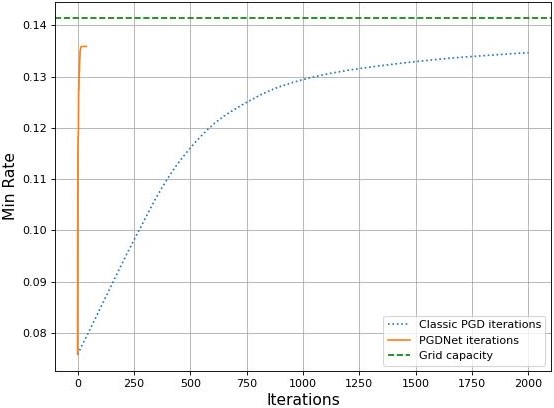
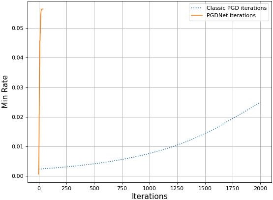
We first consider a case in which the MANET topology remains constant, and evaluate Unfolded PGDNet when given access to the true CSI. Our aim is to assert the ability of our unfolded design to cope with the non-convexity (C1) and the need for rapid tuning (C2). Fig, 5. reports the min-rate of an Unfolded PGDNet with a single model compared with classic PGD versus the iteration number, averaged over all channels, for a noise level of dB for all links. We observe in Fig. 5 that our learn-to-optimize method allows PGDNet to systematically approach the grid capacity with approximately fewer iterations compared to conventional PGD (which requires on average about iterations to converge), demonstrating its ability to cope with C2.
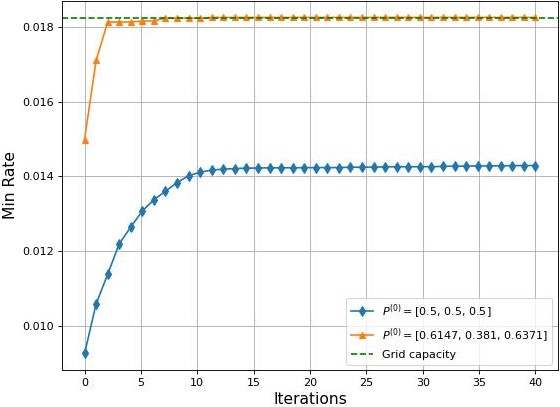
It is noted though that PGDNet with is still within some margin from the grid capacity due to the non-convex nature of the optimization problem (12). This arises as for some of the channel realizations, starting from does not allow to reach the grid capacity. However, when using an alternative initialization, Unfolded PGDNet can rapidly achieve the grid capacity when starting from a different initial guess. This behavior is empirically demonstrated in Fig. 6, confirming the need for our ensemble-based design and its ability to alleviate C1.
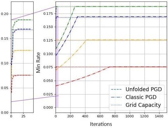
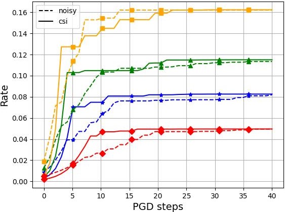
Figs. 5 and 6 indicate the validity of the main ingredients of Unfolded PGDNet, i.e., unfolding for rapid operation and ensemble for coping with non-convexity. We thus proceed by evaluating the overall Unfolded PGDNet using an ensemble of models, where the initial points are randomized uniformly over . The achieved rate versus the number of iterations for four random channel realizations are reported in Fig. 7. This figure demonstrates the robustness of the learned optimizer: for each of the randomly chosen channels, Unfolded PGDNet converged to the grid capacity much faster than the classic PGD. The reduction in latency achieved by Unfolded PGDNet here is of a factor of approximately ( iterations versus required on average for PGD).
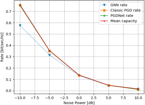
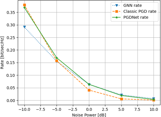
We proceed by evaluating the rate achieved after iterations of Unfolded PGDNet, compared to a data-driven GNN, which is not based on a principled optimizer. Fig. 8 demonstrates that the PGDNet achieves the (mean) grid capacity in various SNR regimes where the GNN fails. In that topology, the classic PGD also achieves grid capacity, but it takes iterations, as opposed to its learned Unfolded PGDNet which achieves this performance within fixed iterations.
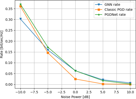
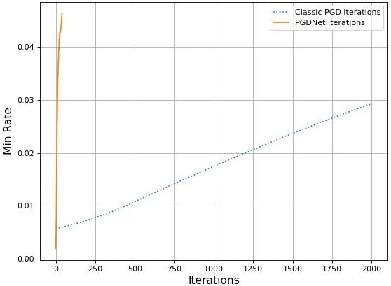
The ability of Unfolded PGDNet to outperform the data-driven GNN is preserved also for the larger MANET, as reported in Fig. 9. For such larger settings, computing the (mean) grid capacity becomes computationally prohibitive. We thus compare the min-rate achieved by three optimizers - classic PGD with 2000 iterations, GNN, and PGDNet with . For every signal-to-noise ratio (SNR) regime, we observe in Fig. 9 that the proposed PGDNet consistently performs the best. It is emphasized that for such larger MANETs, classic PGD converges slower compared to smaller topologies. This behavior is observed in Fig. 10, where the gaps between the learned unfolded algorithm and the fixed step-size version are notably more dominant compared to the smaller MANET reported in Fig. 5.
IV-C Static MANETs with Noisy CSI
We proceed by extending our experimental to the likely setting where there is no access to full CSI data, but instead one must use noisy pilots. We set the number of pilots to be the minimum allowed (i.e., ). As detailed in Subsection III-C, we employ LMMSE estimation to recover the noisy channel estimates as input features to our optimizers. The training procedure uses estimated channels for the inputs during training, while the actual channel realizations are used for computing the loss during training via (20).
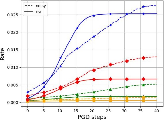
In Fig. 11, we evaluate the rate versus iterations for a noise level of dB. We observe in Fig. 11 that the achieved min-rate is close to the one that was achieved using full CSI in Fig. 10. This indicates that our training method allows Unfolded PGDNet to deal with noisy CSI, converging at a similar rate as that with CSI. Similar findings are also noted when observing the min-rate achieved after learned optimization is concluded for different noise levels. Furthermore, we can see in Fig. 12 that Unfolded PGDNet performs the best among the three algorithms (classic PGD, GNN, and PGDNet) in this scenario as well, preserving the trend observed with full CSI.
While Unfolded PGDNet learns to cope with noisy CSI, its rate is still degraded compared to when processing the true CSI. To showcase this, we report in Fig. 13 the rate versus iteration achieved by PGDNet trained with both full CSI and noisy CSI when applied to full CSI. For comparison, in Fig. 14 we report the rate versus iteration achieved when trained with both full CSI and noisy CSI and applied to noisy CSI. We observe in Fig. 13 that there is indeed some minor degradation due to the processing of noisy channel estimates, yet the noisy training makes PGDNet robust and capable of reliably coping with noisy channel estimates. As expected, Unfolded PGDNet trained using full CSI consistently achieved improved min-data when indeed applied to full CSI, yet the performance gap compared to training with noisy CSI is quite minor. However, in Fig. 14 we observe that noisy-aware training leads to improved robustness. In particular, Unfolded PGDNet trained in a noisy CSI aware manner consistently achieves non-negligible min-rate improvements compared to training using full CSI data, when applied to noisy CSI estimates. These results indicate on the usefulness of our noisy CSI-aware training, and its ability to robustify PGD-based MANET optimization.
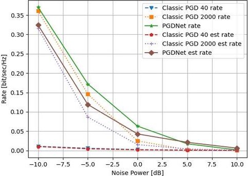
To further demonstrate the robustness of Unfolded PGDNet to noisy CSI, we compare in Fig. 15 classic PGD with Unfolded PGDNet in both scenarios - access to full CSI data and estimated channels (coined est Fig. 15) for different noise levels. We compare three models - Unfolded PGDNet with iterations, classic PGD with iterations, and classic PGD with iterations. We can see in Fig. 15 that the gains of Unfolded PGDNet become more dominant in noisier settings, demonstrating the ability of the proposed methodology to notably facilitate optimizing superposition codes for NOMA MANETs in challenging channel conditions.
IV-D Time-Varying MANETs
A key property of MANETs is their ad-hoc dynamic nature. Accordingly, the network topology, which is typically multi-hop, may change randomly and rapidly over time (corresponding to the block-fading model). As discussed above, the training procedure is based on a given network topology, which is encapsulated in the channel realizations available in the data set (13). Nonetheless, as discussed in Subsection III-B, the learned parameters of PGDNet, i.e., the step-sizes s , are independent of the topology of MANET. This allows Unfolded PGDNet to scale to different MANET sizes.
To showcase the ability of PGDNet to be trained and applied in different topologies, representing time-varying MANET, we simulate a setting where we train on a given topology and use its learned to execute inference (calculating the best power allocation variables) on a different MANET topology. In particular, we train Unfolded PGDNet using channel realizations corresponding to a MANET, and evaluate it on larger MANETs, representing scenarios where additional devices are added to the network. Such settings are conceptually more challenging compared to removing devices, where one can model via a larger MANET while setting relevant links to have zero gain.
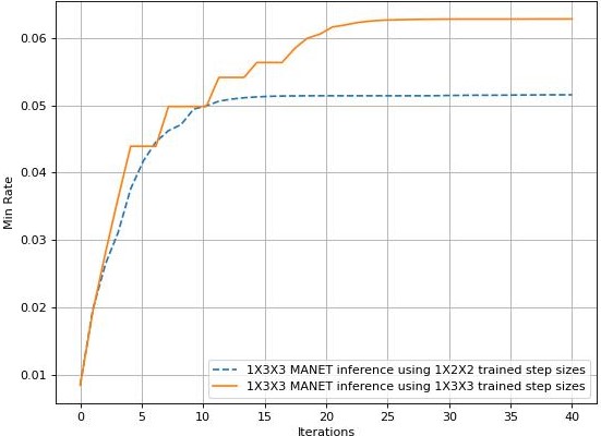
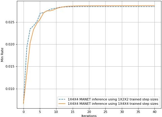
The scalability of Unfolded PGDNet is demonstrated in Figs. 16-17, where we compare the performance achieved by Unfolded PGDNet on topologies having and , respectively, whileused a trained of a network. We observe that Unfolded PGDNet trained on small MANETs manages to reliably scale to larger MANET, achieving performance within a small gap to that achieved when trained for the larger topology. The min-rate gap is more notable for the MANET compared to the , indicating that performance loss is not necessarily due to increasing the size of the MANET, but more likely due to changes in underlying symmetries (which are less profound when going from a MANET to a MANET).
V Conclusion
In this paper, we proposed Unfolded PGDNet for tuning superposition coding in two-hop NOMA MANETs. Unfolded PGDNet leverages data to operate reliably within a fixed and small number of iterations while being trainable in an unsupervised manner. We cope with the non-convexity of the problem by ensemble multiple models. Furthermore, we tackle the practical scenario of using pilots instead of relying on full CSI access successfully through LMMSE estimation. We also manage to overcome the difficulty of the time-varying nature of MANETs by using already trained PGDNet that is empirically proven to be invariant in the manner of the MANET topology. Our numerical results show that Unfolded PGDNet rapidly sets superposition codes that approach the maximal achievable min-rate.
| (21) |
-A Proof of Lemma 1
To prove (16), recall that for any two functions it holds that for every such that . Consequently, computing the objective gradients boils down to (16). Therefore, in order to prove the lemma, we show how (17) is obtained by taking the gradients of (5) and (7).
Here, we derive the complex gradients of with respect to . To that aim, we examine the case where and , and compute the partial derivative where . The gradients for the remaining hops are obtained using a similar derivation.
According to (5), , and . Under this case, we get that the argument of the log expression (which we denote by ) satisfies
By taking the derivative of this equation with respect to , one obtains the formulation in theorem 1 (and specifically of (17a)), as shown in (21) (derived for ). The derivation for the remaining gradients is obtained similarly, thus concluding the proof. ∎
References
- [1] T. Alter and N. Shlezinger, “Deep unfolded superposition coding optimization for two-hop NOMA MANETs,” in IEEE Military Communications Conference (MILCOM), 2023, pp. 286–291.
- [2] M. Wollschlaeger, T. Sauter, and J. Jasperneite, “The future of industrial communication: Automation networks in the era of the internet of things and industry 4.0,” IEEE Ind. Electron. Mag., vol. 11, no. 1, pp. 17–27, 2017.
- [3] W. Chen, J. Liu, H. Guo, and N. Kato, “Toward robust and intelligent drone swarm: Challenges and future directions,” IEEE Netw., vol. 34, no. 4, pp. 278–283, 2020.
- [4] S. H. Cha, M. Shin, J.-H. Ham, and M. Y. Chung, “Robust mobility management scheme in tactical communication networks,” IEEE Access, vol. 6, pp. 15 468–15 479, 2018.
- [5] J. L. Burbank, P. F. Chimento, B. K. Haberman, and W. T. Kasch, “Key challenges of military tactical networking and the elusive promise of MANET technology,” IEEE Commun. Mag., vol. 44, no. 11, pp. 39–45, 2006.
- [6] N. Shlezinger and I. V. Bajic, “Collaborative inference for AI-empowered IoT devices,” IEEE Internet of Things Magazine, vol. 5, no. 4, pp. 92–98, 2022.
- [7] A. El Gamal and Y.-H. Kim, Network information theory. Cambridge university press, 2011.
- [8] Y. Liu, Z. Qin, M. Elkashlan, Z. Ding, A. Nallanathan, and L. Hanzo, “Nonorthogonal multiple access for 5G and beyond,” Proc. IEEE, vol. 105, no. 12, pp. 2347–2381, 2017.
- [9] Z. Ding, X. Lei, G. K. Karagiannidis, R. Schober, J. Yuan, and V. K. Bhargava, “A survey on non-orthogonal multiple access for 5G networks: Research challenges and future trends,” IEEE J. Sel. Areas Commun., vol. 35, no. 10, pp. 2181–2195, 2017.
- [10] J. G. Andrews, “Interference cancellation for cellular systems: a contemporary overview,” IEEE Wireless Commun., vol. 12, no. 2, pp. 19–29, 2005.
- [11] T. V. Loung, N. Shlezinger, T. M. H. C Xu, Y. C. Eldar, and L. Hanzo, “Deep learning based successive interference cancellation for the non-orthogonal downlink,” IEEE Trans. Veh. Technol., vol. 71, no. 11, pp. 11 876–11 888, 2022.
- [12] Y. Gao, B. Xia, K. Xiao, Z. Chen, X. Li, and S. Zhang, “Theoretical analysis of the dynamic decode ordering SIC receiver for uplink NOMA systems,” IEEE Commun. Lett., vol. 21, no. 10, pp. 2246–2249, 2017.
- [13] N. Shlezinger, R. Fu, and Y. C. Eldar, “DeepSIC: Deep soft interference cancellation for multiuser MIMO detection,” IEEE Trans. Wireless Commun., vol. 20, no. 2, pp. 1349–1362, 2021.
- [14] M. Jain, N. Sharma, A. Gupta, D. Rawal, and P. Garg, “Performance analysis of NOMA assisted mobile ad hoc networks for sustainable future radio access,” IEEE Sustain. Comput., vol. 6, no. 2, pp. 347–357, 2020.
- [15] A. Amer, S. Hoteit, and J. Ben-Othman, “Resource allocation for enabled-network-slicing in cooperative NOMA-based systems with underlay D2D communications,” in IEEE International Conference on Communications (ICC), 2023.
- [16] A. Chowdhury, G. Verma, C. Rao, A. Swami, and S. Segarra, “ML-aided power allocation for tactical MIMO,” in IEEE Military Communications Conference (MILCOM), 2021, pp. 273–278.
- [17] L. Schynol and M. Pesavento, “Coordinated sum-rate maximization in multicell MU-MIMO with deep unrolling,” IEEE J. Sel. Areas Commun., vol. 41, no. 4, pp. 1120–1134, 2023.
- [18] T. Chen, X. Chen, W. Chen, Z. Wang, H. Heaton, J. Liu, and W. Yin, “Learning to optimize: A primer and a benchmark,” The Journal of Machine Learning Research, vol. 23, no. 1, pp. 8562–8620, 2022.
- [19] N. Shlezinger and Y. C. Eldar, “Model-based deep learning,” Foundations and Trends® in Signal Processing, vol. 17, no. 4, pp. 291–416, 2023.
- [20] N. Shlezinger, J. Whang, Y. C. Eldar, and A. G. Dimakis, “Model-based deep learning,” Proc. IEEE, vol. 111, no. 5, pp. 465–499, 2023.
- [21] N. Shlezinger, Y. C. Eldar, and S. P. Boyd, “Model-based deep learning: On the intersection of deep learning and optimization,” IEEE Access, vol. 10, pp. 115 384–115 398, 2022.
- [22] O. Sagi and L. Rokach, “Ensemble learning: A survey,” Wiley Interdisciplinary Reviews: Data Mining and Knowledge Discovery, vol. 8, no. 4, p. e1249, 2018.
- [23] Y. Shen, J. Zhang, S. Song, and K. B. Letaief, “Graph neural networks for wireless communications: From theory to practice,” IEEE Trans. Wireless Commun., vol. 22, no. 5, pp. 3554–3569, 2023.
- [24] D. Tse and P. Viswanath, Fundamentals of wireless communication. Cambridge university press, 2005.
- [25] B. Hassibi and B. M. Hochwald, “How much training is needed in multiple-antenna wireless links?” IEEE Trans. Inf. Theory, vol. 49, no. 4, pp. 951–963, 2003.
- [26] N. Shlezinger and Y. C. Eldar, “On the spectral efficiency of noncooperative uplink massive MIMO systems,” IEEE Trans. Commun., vol. 67, no. 3, pp. 1956–1971, 2019.
- [27] A. Papoulis and S. U. Pillai, Probability, random variables, and stochastic processes. McGraw-Hill Europe: New York, NY, USA, 2002.
- [28] S. P. Boyd and L. Vandenberghe, Convex optimization. Cambridge university press, 2004.
- [29] O. Lavi and N. Shlezinger, “Learn to rapidly and robustly optimize hybrid precoding,” IEEE Trans. Commun., vol. 71, no. 10, pp. 5814–5830, 2023.
- [30] W. Wang and M. A. Carreira-Perpinán, “Projection onto the probability simplex: An efficient algorithm with a simple proof, and an application,” arXiv preprint arXiv:1309.1541, 2013.
- [31] N. Parikh, S. Boyd et al., “Proximal algorithms,” Foundations and trends® in Optimization, vol. 1, no. 3, pp. 127–239, 2014.
- [32] N. Shlezinger and T. Routtenberg, “Discriminative and generative learning for linear estimation of random signals [lecture notes],” IEEE Signal Process. Mag., vol. 40, no. 6, pp. 75–82, 2023.
- [33] N. Samuel, T. Diskin, and A. Wiesel, “Learning to detect,” IEEE Trans. Signal Process., vol. 67, no. 10, pp. 2554–2564, 2019.
- [34] Y. Noah and N. Shlezinger, “Limited communications distributed optimization via deep unfolded distributed ADMM,” arXiv preprint arXiv:2309.14353, 2023.
- [35] D. P. Kingma and J. Ba, “Adam: A method for stochastic optimization,” arXiv preprint arXiv:1412.6980, 2014.