Structured Learning of
Compositional Sequential Interventions
Abstract
We consider sequential treatment regimes where each unit is exposed to combinations of interventions over time. When interventions are described by qualitative labels, such as “close schools for a month due to a pandemic” or “promote this podcast to this user during this week”, it is unclear which appropriate structural assumptions allow us to generalize behavioral predictions to previously unseen combinatorial sequences. Standard black-box approaches mapping sequences of categorical variables to outputs are applicable, but they rely on poorly understood assumptions on how reliable generalization can be obtained, and may underperform under sparse sequences, temporal variability, and large action spaces. To approach that, we pose an explicit model for composition, that is, how the effect of sequential interventions can be isolated into modules, clarifying which data conditions allow for the identification of their combined effect at different units and time steps. We show the identification properties of our compositional model, inspired by advances in causal matrix factorization methods but focusing on predictive models for novel compositions of interventions instead of matrix completion tasks and causal effect estimation. We compare our approach to flexible but generic black-box models to illustrate how structure aids prediction in sparse data conditions.
1 Contribution
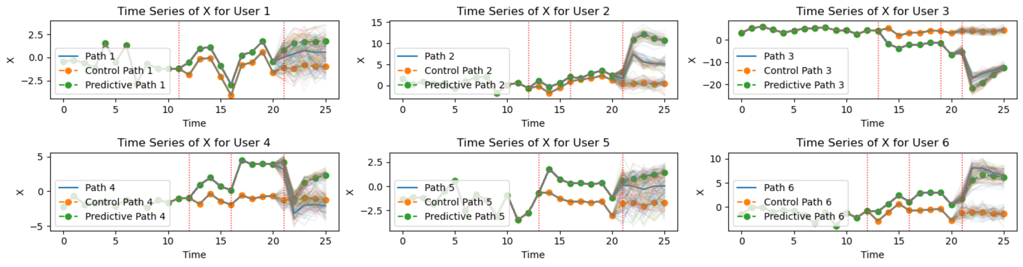
Many causal inference questions involve a treatment sequence that varies over time. In the (discrete) time-varying scenario, an unit is exposed to a sequence of treatments controlled by an external agent (Hernán and J, 2020, Ch. 19). Each can be interpreted as a cause of the subsequent behavior , and its modeling amenable to the tools of causal inference (e.g., Robins, 1986, 1997; Murphy, 2003; Didelez et al., 2006; Chakraborty and Moodie, 2013; Zhang and Bareinboim, 2020). For instance, each can take values in the space of particular drug dosages which can be given to an in-patient, or combinations of items to be promoted to a user of a recommender system. Here, patients and users are the units, and denotes a measure of their state or behavior under time . Dependencies can result in a dense causal graph, as in Fig. 1. Further background on this classical problem is provided in Appendix A.
Scope.
We introduce an approach to model the effects of a combinatorial and sparse space of intervention sequences, including the bursts of non-stationarity that the application of an intervention brings in. We consider the case where each behaves as if it was randomized to focus on predictive guarantees on large, possibly underspecified, sequential action spaces. We will consider neither experimental design nor reinforcement learning, instead focusing on the problem of behavioral forecasting under hypothetical future interventions given past controlled interventions.
Challenges and prior work.
Much of the sequential intervention literature in AI and statistics considers generic models111We include here models which explicit parameterize causal contrasts in longitudinal interventions, such as the blip models of Robins (1997). to map sequences to behavior and beyond, sometimes exploiting strong Markovian assumptions or short sequences and small action spaces (Chakraborty and Moodie, 2013; Sutton and Barto, 2018). An unstructured black-box for sequences, such as recurrent neural networks and their variants (e.g. Hochreiter and Schmidhuber, 1997; Cho et al., 2014; Vaswani et al., 2017), can learn to map a sequence to a prediction. This is less suitable when interventions are categorical and sparse, with most entries corresponding to some baseline category of “no changes”. That is, there is no obvious choice of smoothing or interpolation criteria to generalize from seen to unseen strings , with the practical assumption being that we see enough variability to reliably perform this interpolation. There is an increased awareness of problems posed by large discrete spaces among pre-treatment covariates (Yao et al., 2019; Zeng et al., 2024), which is of a different nature as losses can be minimized with respect to an existing natural distribution, as opposed to the interventional problem where the design variables are allowed to be chosen and so sparsity conditions can easily result in very atypical test cases of interest. Several papers address large intervention spaces (mostly for non-sequential problems) without particular concerns about non-smooth, combinatorial identifiability (Kaddour et al., 2021; Nabi et al., 2022; Saito et al., 2023, 2024). A few more recent papers address explicit assumptions of identifiability directly in combinatorial categorical spaces by sparse regression (Agarwal et al., 2023a) or energy functions Bravo-Hermsdorff et al. (2023), but without a longitudinal component. More classically, tools like the do-calculus (Pearl, 2009) and their extensions (Correa and Bareinboim, 2020) can be used with directed acyclic graphs (DAGs) to infer combinatorial effects, although they often restrict each intervention variable to target a single random variable (e.g. Aglietti et al. (2020)). With strong assumptions and computation, this may include latent variables Zhang et al. (2023). Alternative representation learning ideas for carefully extrapolating to unseen interventions are presented by (Saengkyongam et al., 2024) in the non-sequential setting.
In this paper, we consider the conservative problem of identification guarantees for the effect of sequential combinations of interventions which may never have co-occurred jointly in training data, formalizing assumptions that allows for the transfer and recombination of information learned across units. These are not of the same nature as identifiability of causal effects from observational data (Pearl, 2009) or causal discovery (Spirtes et al., 2000), but of causal extrapolation: even in the randomized (or unconfounded) regime, it is not a given that the distribution of a particular potential outcome can be reliably inferred from limited past combinations of interventions without an explicit structure on the causal generative model. We will consider the case where interventions have non-stationary effects: once unit is exposed to , then will have dynamics that can be affected not only by the choice of but also the difference , resulting in dense dependency structures such as the one in Figure 1. As multiple treatments are applied to the same unit , there will be a composition of effects that will depend not only on the labels of the interventions, but also on the order by which they take place. If a substantive number of choices of interventions at time is available, a large dataset may have no two sequences and taking the same values, even when considering only the unique treatment values applied and regardless of ordering and time stamps.
Problem statement.
Let each individual unit be described by time-invariant features and a pair of time-series . Each is a categorical variable representing an intervention (also called treatment, or exposure), encoded by values in , and sequentially unconfounded with the system by randomization or assumption. describes an intervention which causes changes to the distribution of , the time-series of state variables starting at time . The special value denotes an “idle” or “default” treatment that can be interpreted as “no intervention”. Given a training set of units and observations up to a time point , the goal is to predict future sequence of states for an unit under a hypothetical intervention . We denote it as , where denotes a slice of a discrete-time time series of random vectors from to , inclusive; is the potential outcome (Imbens and Rubin, 2015; Hernán and J, 2020; Pearl, 2009) of variable under interventions . This process takes place under stable unit treatment value assumption (SUTVA) (Imbens and Rubin, 2015), meaning that interventions only affect unit .
Each intervention is allowed to have an impact on the whole future series . It can correspond to an instantaneous shock (“give five dollars of credit at time ”) or an action that takes place over an extended period of time (“promote this podcast from time to time ”): we just assume the meaning to be directly encoded within arbitrary category labels . In a real-world scenario where a same action can be applied more than once, different symbols in should be used for each instance (e.g., 1 arbitrarily standing for “give five dollars”, and 2 for “give five dollars a second time” and so on).
In Section 2, we provide an account of what we mean by compositionality of interventions, with explicit assumptions for identifiability. In Section 3, we describe an algorithm for likelihood-based learning, along with approaches for predictive uncertainty quantification. Further related work is covered in Section 4 before we perform experiments in Section 5, highlighting the shortcomings of black-box alternatives.
2 A Structural Approach for Intervention Composition
For simplicity, we will assume scalar behavioral measurements , as the multivariate case readily follows. Consider the following conditional mean model for the potential outcome ,
| (1) |
where is the elementwise product, for any (future interventions do not affect past outcomes), and for all . We do not explicitly condition on in most of our notation, adopting a convention where potential outcome indices are always in agreement with the (implicit) corresponding observed . We define as evaluations of basis functions , which for now we will assume to be known. Each individual has their individual-level coefficients . Causal impact, as attributed to , is given by
| (2) |
where function captures a trajectory in time for the effect of , for . We consider two variants. The first is a time-bounded variant which, for , defines , where is a free parameter for , otherwise . The intuition is that the effect of intervention level has no shape constraints but it cannot affect the past and it must settle to a constant after a chosen time window hyperparameter . The default level has no effect and no free parameters, with . The second variant is motivated by real-world phenomena where causal impacts diminish their influence over time and result in a new equilibrium (Brodersen et al., 2015). We consider a time-unbounded shape with exponential decay, parameterized as
| (3) |
where is the sigmoid function, so that . As grows, goes to 0. is the stationary contribution of an intervention at level . In particular, for , we define and , while for we have that , and are free parameters to be learned. By defining as the dimensionality of intervention level , we adopt the convention for the prescribed time-unbounded model of Eq. (3).
2.1 Representation Power and Compositional Warping
Eq. (1) is reminiscent of tensor factorization and its uses in causal modeling (Athey et al., 2021; Agarwal et al., 2023b), where the primary motivation comes from the imputation of missing potential outcomes taking place on a pre-determined period in the past. From a predictive perspective, it can be motivated from known results in functional analysis (such as Proposition 1 of (Kaddour et al., 2021)) that allows us to represent a function by first partitioning its input into and controlling the approximation error given by an inner product of vector-valued functions , in practice choosing the dimensionality of the vectors by a data-driven approach. Although those results apply typically to smooth functions with continuous inputs (such as the Taylor series approximation, which relies on vectors of monomials with coefficients constructed from derivatives), discrete inputs such as e.g. at a fixed dimensionality can be separated from the other inputs as . Here, similarly to classical ANOVA models, is a one-hot encoding vector for the entire (exponentially sized) space of possible trajectories, and returns a vector of corresponding length.
As we do not want to restrict ourselves to fixed (and ), not to mention an exponential cost of representation, we will resort to fixed-dimensional embeddings of sequences and identities. In particular, we design to have a finite output dimensionality . Inspired by sequential hidden representation models such as recurrent neural networks, we define , for , via the following recursive definition on :
| (4) |
such that for any (that is, intervention level does nothing) and for any (base case). A representational choice requires a choice of dimensionality for the inner vectors . Recursively applying (4) in this product form can still be done relatively efficiently, but choosing for all simplifies matters as we apply again the inner product formula to to get to a factorization form analogous to Eq. (1). More formally:
Proposition 1
Let , where function sequences and are defined for all and have codomain . Furthermore, define as in Eq. (4) with , and the -th entry of as , each of the latter having codomain and where is defined recursively for any , similarly . Then there exists some integer and three functions and with codomain so that . Moreover for functions .
Proofs of this and next results are given in Appendix B. The above shows that if we start with an assumption that the ground truth function takes some desired form, then there is some finite for which our combination of basis functions can parameterize the ground truth function for arbitrary , analogous to in Eq. (1). On the other hand, we show a companion result below, that if we hold fixed, there is some fixed value for , which depends polynomially on , such that any measurable ground truth function can be approximated by our combination of some appropriate choice of basis functions. This is reminiscent of the line of work on matrix factorization (e.g., Appendix A of Agarwal et al. (2023c)).
Proposition 2
Given a fixed value of , suppose we have a measurable function , , where and are compact, is finite. For , let with . For every there exist such that for any , there are measurable functions and and real numbers for and , such that
| (5) |
Notes.
Eq. (1) and Eq. (2) are motivated by the success of approaches for representation learning of sequences, which assumes that we can compile all the necessary information from the past using a current finite representation at any time step . However, knowledge of Propositions 1 and 2 further imply that, for , the representation of functions in a multilinear combination of adaptive factors (Eq. (1)) is motivated by more fundamental results in functional analysis. Our assumption that no value of (other than the baseline 0) can be used more than once has mostly an empirical motivation, as this would imply unrealistic assumptions about the same intervention having the same effect when applied multiple times. Ultimately, we assume that the factors leading to Eq. (2) are time-translation invariant, being a function of and only. While it is possible to generalize beyond translation invariant models, as commonly done in the synthetic controls literature (Abadie, 2021) that inspired the causal matrix factorization ideas (Athey et al., 2021; Agarwal et al., 2023b, c), this would complicate matters further by requiring a fourth factor into the summation term of Eq. (1) to encode absolute time. Models for time-series forecasting with parameter drifts can be tapped into and integrated with our model family, but we leave these out as future work.
Interpretation.
At the starting of the process, where all units are assumed to be at their “natural” state (assuming ), we can interpret as a finite basis representation, with respect to , of . Each can be seen as a latent feature of unit . Effect vector defines a warping of that describes how treatments affect the behaviour of an individual with the resulting . The modifier can be interpreted as reverting, suppressing or promoting particular latent features that are assumed to encode all information necessary to reconstruct the conditional expectation of from the chosen basis (notice that intervention level 0 implies since we define ). This presents a sequential warping view of compositionality of interventions.
2.2 Identification and Data Assumptions
Assume for now that functions are known. As common in the literature of matrix factorization, assume also that we have access to some moments of the distribution. In particular, for given data points and time points, we have access to . We will impose conditions on the realizations of and values chosen for , as well as values of and as a function of , in order to identify each and the parameters of for all intervention levels of interest. The theoretical results presented, which describe how parameters are identifiable from population expectations and known function spaces determined by a prescribed basis of known and finite dimensionality , will then provide a basis for a practical learning algorithm in the sequel.
Assumption 1
For a given individual , we assume there is an initial period with “no interventions” i.e., for all .
Assumption 2
let be a matrix where each row is given by . We assume that is full rank with left pseudo-inverse .
Assumption 3
For a given intervention level , assume for all and that there is at least one time index , and one set containing all units where , such that: (i) ; (ii) , where is the dimensionality of the intervention level .
Assumption 4
Let index the elements of a set of units . For , let be a matrix where each row is given by . We assume that each is full rank with left pseudo-inverse .
This leads to the main result of this section:
Theorem 1
Assume we have a dataset of units and time points generated by a model partially specified by Eq. (1). Assume also knowledge of the conditional expectations and basis functions for all and all and . Then, under Assumptions 1-4 applied to all individuals and all intervention levels that appear in our dataset, we have that all and all are identifiable.
Notice that nothing above requires prior knowledge of all intervention levels which will exist, and could be applied on a rolling basis as new interventions are invented. There is no need for all units to start synchronously at : the framing of the theory assumes so to simplify presentation, but the only requirement is that each unit is given a “burn-in” period of at least steps and that each new intervention level is applied to at least units which have not been perturbed recently by relatively novel interventions (that is, units which, if they were given a past intervention not given to anyone else before, then that perturbation should have taken place enough steps in the past so that all recent but past functions have been identified).
3 Algorithm and Statistical Inference
This section introduces a learning algorithm, and well as ways of quantifying uncertainties in prediction. We also allow for the learning of adaptive basis functions . As Eq. (1) does not define a generative model, which will be necessary for multiple-steps-ahead prediction, for the remainder of this section we will assume the likelihood implied by . Here, the conditional mean is given by Eq. (1) and , an error unaffected by and other variables. Hence, requires no further needs for identification results. In general, if our likelihood is defined via a finite set of estimating equations, we can parameterize it in the multilinear form analogous to (1) and repeat the analysis of the previous section. In practice, the functionals (such as the conditional expectations of ) used in an estimating equation are unknown. Matrix factorization methods can be applied directly by first performing a smoothing method on the data to get plug-in estimates of these functionals Squires et al. (2022), but we will adopt instead a likelihood-based approach.
3.1 Algorithm: CSI-VAE
We treat each as a random effects vector, giving each entry an independent zero-mean Gaussian prior with variance . Along with all hyperparameters, we optimize the (marginal) log-likelihood by gradient-based optimization. With a Gaussian likelihood, the posterior and filtering distribution of each can be computed in closed form, but in our implementation we used a black-box amortised variational inference framework (Kingma and Welling, 2013; Mnih and Gregor, 2014; Rezende et al., 2014) anyway that can be readily put together without specialized formulas and is easily adaptable to other likelihoods. We use a mean-field Gaussian approximation with posterior mean and variances produced by a gated recurrent unit (GRU) model (Chung et al., 2014) composed with a multilayer perceptron (MLP). The approximate posterior parameters at sample with time steps are therefore and . Prediction for is done by sampling trajectories, where for each trajectory we first sample a new from the mean-field Gaussian approximation. We set each forward to be the corresponding marginal Monte Carlo average. Each basis vector is parameterized via another GRU model such that . Although the theory in the previous section relies on known basis functions, we could train this GRU up to an threshold time point and freeze it from that point, each being defined as the unit coefficient vector for this basis. In practice, we found that doing end-to-end learning provides a modest improvement, and this will be the preferred approach in the experiments. We do find that sometimes it is more stable to only use time series up to time point for the amortized inference. Hence, we adopt this pipeline for any results reported in this paper, unless otherwise specified. We call our method Compositional Sequential Intervention Variational Autoencoder (CSI-VAE).
3.2 Distribution-free Uncertainty Quantification
Conformal prediction (CP) Vovk et al. (2005); Fontana et al. (2023) provides prediction intervals with coverage guarantees. The intervals are computed using a calibration set of labeled samples and include the future samples with non-asymptotic lower-bounded probability. We consider Split Conformal Prediction in two setups.
-
1.
Hold-out predictions. We have a set of historical users, , whose behaviour has been observed until time . The task is to predict the behaviour at time of a new user, , who has been observed up to time , i.e. to predict given and . If we assume we have used the history of the new user , , to train the model, calibration and test samples are exchangeable.
-
2.
Next-intervention predictions. We have observed the behaviour of all users, , up to time and aim to predict the effects of the next intervention, which happens at time for all users, i.e. , holding . The task is to predict for , but in what follows we will drop the potential outcome notation to keep notation lighter, referring to observed . Calibration and test are not exchangeable, because i) the joint distribution after time , may be different from the one before time , , and ii) we only used , , for training.
CP algorithms are applied on top of given point-prediction models. In our case, the underlying model is , which predicts the expected user behaviour at time given the user history up to time , i.e. .
Setup 1.
Calibration and test scores, and are exchangeable, i.e. where is any permutation of . The Quantile Lemma, e.g. Lemma 1 of Tibshirani et al. (2019), implies the prediction interval
| (6) | ||||
is valid in the sense it obeys
| (7) |
where the probability is over the calibration and test samples.
Setup 2.
The prediction intervals defined in (6) may not be valid, i.e. (7) may not hold, because the calibration and test samples, with and , , are not exchangeable. Theorem 2 provides a bound on the coverage gap, i.e. a measure of violation of (7), under the assumption that the distribution shift is controlled by a perturbation parameter, .
Theorem 2
Assume we have calibration samples,
| (8) |
where is the time user experienced the last intervention before . Assume there exists such that, for all ,
| (9) |
where and are the (unknown) densities of the test and calibration distributions, is a bounded arbitrary shift density, and . Then,
| (10) |
In the proof, we use the likelihood-ratio-weighting approach of Tibshirani et al. (2019) to obtain the empirical test distribution from the calibration samples and bound its quantile from below. The statement follows from standard inequalities on the mean and variance of the -perturbed distribution. We prefer this approach to conformal prediction adaptive models for time series, e.g. Gibbs and Candes (2021) or Angelopoulos et al. (2024), for two reasons: i) adaptive schemes have asymptotic coverage guarantees that can not be used to estimate the uncertainty on a single time step and ii) optimised density estimates are a byproduct of our prediction model.
4 Further Related Work
Brodersen et al. (2015) leverages Bayesian structural time-series models to estimate causal effects, and motivates our exponential decay model in Eq. (3). Unlike Brodersen et al. (2015), who focus on single interventions, our model explicitly addresses the complexity arising from sequential interventions, providing a more detailed perspective on the dynamic interplay of treatments over time. Several approaches for conformal prediction in causal inference have emerged in recent years (e.g., Tibshirani et al., 2019; Lei and Candès, 2021), including matrix completion Gui et al. (2023) and synthetic controls Chernozhukov et al. (2021). Our focus has not been on individual nor average treatment effects, but directly on expected potential outcomes, similarly to the work on causal matrix completion Athey et al. (2021); Agarwal et al. (2023b, c); Squires et al. (2022). Unlike the matrix completion literature, we focused on prediction problems, out-of-sample for both units and time steps. Moreover, the matrix completion literature is usually framed in terms of marginal expectations , as opposed to conditional expectations (notice that Agarwal et al. (2023c) considers covariates, but those are included as part of the generative model). Marginal models have some advantages when modeling multiple-step-ahead effects Evans and Didelez (2024), but they also involve complex computational considerations that we leave for future work. Finally, there is a rich literature on confounding adjustment where exogeneity of cannot be assumed, see Hernán and J (2020) for a textbook treatment. Some of the causal matrix completion literature takes the perspectiven that factors such as could be interpreted as latent factors conditional on which ignorability could be assumed. However, we consider this assumption hard to justify due to the unknown nature of . We can rely on standard approaches of sequential ignorability Robins (1997) to justify our method in the absence of randomization.
5 Experiments
We run a number of synthetic and semi-synthetic experiments to evaluate the performance of the CSI-VAE approach. In this section, we summarize our experimental set-up and main results. The code for reproducing all results and figures is available online222The code will be released upon acceptance, and is available in the supplementary material.; in Appendix C, we provide a detailed description of the datasets and models; in Appendix D, we present further analysis and more results; and in Appendix E we present a demo for uncertainty quantification results.
| Full Synthetic | Semi-Synthetic Spotify | |||||||||
|---|---|---|---|---|---|---|---|---|---|---|
| Model | T+1 | T+2 | T+3 | T+4 | T+5 | T+1 | T+2 | T+3 | T+4 | T+5 |
| CSI-VAE-1 | ||||||||||
| CSI-VAE-2 | ||||||||||
| CSI-VAE-3 | ||||||||||
| GRU-0 | ||||||||||
| GRU-1 | ||||||||||
| GRU-2 | ||||||||||
|
|
|
|
| Full Synthetic | Semi-Synthetic Spotify | |||||||||
|---|---|---|---|---|---|---|---|---|---|---|
| Model | CSI-VAE-2 | CSI-VAE-3 | GRU-0 | GRU-1 | GRU-2 | CSI-VAE-2 | CSI-VAE-3 | GRU-0 | GRU-1 | GRU-2 |
| CSI-VAE-1 | ||||||||||
| CSI-VAE-2 | ||||||||||
| CSI-VAE-3 | ||||||||||
| GRU-0 | ||||||||||
| GRU-1 | ||||||||||
Datasets and oracular simulators.
The first step to assess intervention predictions is to build a set of proper ground truth test beds, where we can control different levels of combinations of interventions. We build two sets of oracular simulators. (1) The Fully-synthetic simulator is constructed primarily based on random models following our parameterization in Section 2. (2) The Semi-synthetic simulator is constructed based on a real-world dataset from Spotify333https://open.spotify.com/ which is aims to predict skip behaviour of users based on its past interaction history. See details in Appendix C. For each type of simulator, we generate different versions with different random seeds. From simulator (1), we construct a simulated datasets of size , containing different interventions happening to the units at any time after an initial burn-in period of , although only maximum of these can be observed for any given unit, with being the true dimensions of the model. For simulator (2), we construct simulated datasets of size , again containing different interventions, an initial period , a maximum 3 different interventions per unit and . For making predictions, we predict outcomes for interventions not applied yet within any given unit (i.e. at least from the options left). In simulator (2) parameters and are learned from real-world data. Interventions are artificial, but inspired by the process of showing different proportions of track types to an user in a Spotify-like environment. For both setups, we use a data ratio of for training, validation and test, respectively. We report the final results in Table 1 with another constructed holdout set ( for fully-synthetic and for semi-synthetic).
Compared models.
We implemented three variations: (1) CSI-VAE-1 follows exactly our setup in Section 2; (2) CSI-VAE-2 can be considered as an ablation study, which relaxes the product form of Eq. 1 and replace it with a black-box MLP applied directly to (and hence may not guarantee identifiability); (3) CSI-VAE-3 as another ablation study, where the equation for (Eq. (2)) is replaced by a black-box function taking the sequence of interventions as a standard time series. We compare our model against: (1) GRU-0, a black-box gated recurrent unit (GRU, Cho et al. (2014)) composed with a MLP, using only the past history of and ; (2) GRU-1, another GRU composed with a MLP that takes into account also the latest intervention ; and (3) GRU-2, which uses not only but also the entire past history just like CSI-VAE. In general, GRU-2 can be considered as a very strong and generic black-box baseline model.
Results.
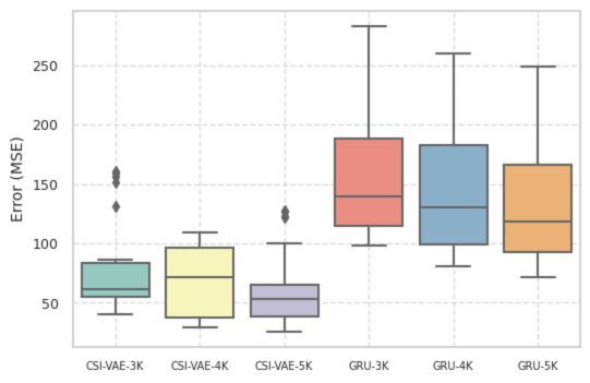
Each experiment was repeated 5 times, using Adam Kingma and Ba (2015) at a learning rate of 0.01, with 50 epochs in the fully-synthetic case and 100 for the semi-synthetic, which was enough for convergence. We selected the best iteration point based on small holdout set. The main results are presented in Tables 1 and 2, which shows the superiority of our model against the strong baselines. We also observed that the identifiable results and compositional interactions of intervention effect are both critical, as evidenced by the drop in performance for CSI-VAE 2 and 3 in Table 1. In Appendix D, we provide the following further experiments: (1) different choices of (to summarize: using less than the true value gracefully underfits, while there is evidence of small overfitting for choices of which overshoot the true value but where we can enforce regularization techniques; (2) different size of the training data (to summarize: even with more data provided, our model consistently outperforms the blackbox models by a significant margin. We show that a generic blackbox cannot solve this problem by simply feeding in more data); and (3) a demonstration of conformal prediction that allow us to better calibrate the predictive coverage compared to vanilla model-based prediction.
6 Conclusion
We introduced an approach for predicting potential outcomes with a careful accounting of when extrapolation to unseen sequences are warranted. Lessons. Embeddings are important given sparse categorical sequential data see e.g. (Vaswani et al., 2017). However, large combinatorial interventional spaces benefit from models that more carefully lay down conditions for identification. Limitations. Unlike the traditional synthetic control literature Abadie (2021), we assume a model for time effects based on autoregression and truncated or parametric temporal-intervention interactions. While it is possible to empirically evaluate the prediction abilities of the model using a validation sample, high-stakes applications (such as major interventions to counteract the effect of a pandemic) should take into consideration that uncontrolled distribution shifts may take place, and careful modeling of such shifts should be added to any analytical pipeline to avoid damaging societal implications. Future Work. Besides allowing for an explicit parameterization of drifts, an explicit account for modeling when unmeasured confounding may have been presented in the selection of past interventions is necessary to increase the applicability of the method to more sources of data.
Acknowledgements
We thank Zhenwen Dai and Georges Dupret for many helpful comments and suggestions. JY and RS were partially funded by the EPSRC Open Fellowsship EP/W024330/1. RS acknowledges further funding from the EPSRC AI Hub for Causality in Healthcare AI with Real Data, EP/Y028856/1.
References
- Abadie [2021] A. Abadie. Using synthetic controls: Feasibility, data requirements, and methodological aspects. Journal of Economic Literature, 59:391–425, 2021.
- Agarwal et al. [2023a] A. Agarwal, A. Agarwal, and S. Vijaykumar. Synthetic combinations: A causal inference framework for combinatorial interventions. Advances in Neural Information Processing Systems 36 (NeurIPS 2023), pages 19195–19216, 2023a.
- Agarwal et al. [2023b] A. Agarwal, M. Dahleh, D. Shah, and D. Shen. Causal matrix completion. Proceedings of Thirty Sixth Conference on Learning Theory, pages 3821–3826, 2023b.
- Agarwal et al. [2023c] A. Agarwal, D. Shah, and D. Shen. Synthetic interventions. arXiv:2006.07691 (econ), 2023c.
- Aglietti et al. [2020] V. Aglietti, X. Lu, A. Paleyes, and J. Gonz’alez. Causal Bayesian optimization. Proceedings of the Twenty Third International Conference on Artificial Intelligence and Statistics, 34:3155–3164, 2020.
- Angelopoulos et al. [2024] Anastasios Angelopoulos, Emmanuel Candes, and Ryan J Tibshirani. Conformal pid control for time series prediction. Advances in Neural Information Processing Systems, 36, 2024.
- Athey et al. [2021] S. Athey, M. Bayati, N. Doudchenko, G. Imbens, and K. Khosravi. Matrix completion methods for causal panel data models. Journal of the American Statistical Association, 116:1716–1730, 2021.
- Bravo-Hermsdorff et al. [2023] G. Bravo-Hermsdorff, D. Watson, J. Yu, J. Zeitler, and R. Silva. Intervention generalization: A view from factor graph models. Advances in Neural Information Processing Systems 36 (NeurIPS 2023), pages 43662–43675, 2023.
- Brodersen et al. [2015] K. Brodersen, F. Gallusser, J. Koehler, N. Remy, and S. Scott. Inferring causal impact using Bayesian structural time-series models. Annals of Applied Statistics, to appear, 2015.
- Brost et al. [2019] Brian Brost, Rishabh Mehrotra, and Tristan Jehan. The music streaming sessions dataset. In The World Wide Web Conference, pages 2594–2600, 2019.
- Chakraborty and Moodie [2013] B. Chakraborty and E. Moodie. Statistical Methods for Dynamic Treatment Regimes: Reinforcement Learning, Causal Inference, and Personalized Medicine. Springer, 2013.
- Chernozhukov et al. [2021] Victor Chernozhukov, Kaspar Wuthrich, and Yinchu Zhu. An exact and robust conformal inference method for counterfactual and synthetic controls. Journal Of The American Statistical Association, 116(536):1849–1864, OCT 2 2021. ISSN 0162-1459. doi: 10.1080/01621459.2021.1920957.
- Cho et al. [2014] K. Cho, B. van Merriënboer, C. Gulcehre, D. Bahdanau, F. Bougares, H. Schwenk, and Y. Bengio. Learning phrase representations using RNN encoder–decoder for statistical machine translation. Proceedings of the 2014 Conference on Empirical Methods in Natural Language Processing (EMNLP 2014), pages 1724–1734, 2014.
- Chung et al. [2014] Junyoung Chung, Caglar Gulcehre, KyungHyun Cho, and Yoshua Bengio. Empirical evaluation of gated recurrent neural networks on sequence modeling. arXiv preprint arXiv:1412.3555, 2014.
- Correa and Bareinboim [2020] J. Correa and E. Bareinboim. A calculus for stochastic interventions:causal effect identification and surrogate experiments. Proceedings of the AAAI Conference on Artificial Intelligence (AAAI 2020), 34:10093–10100, 2020.
- Dawid [2021] P. Dawid. Decision-theoretic foundations for statistical causality. Journal of Causal Inference, 9(56):39–77, 2021.
- Didelez et al. [2006] V. Didelez, A. P. Dawid, and S. Geneletti. Direct and indirect effects of sequential treatments. Proceedings of the Twenty-Second Conference on Uncertainty in Artificial Intelligence (UAI2006), 2006.
- Evans and Didelez [2024] R. Evans and V. Didelez. Parameterizing and simulating from causal models. Journal of the Royal Statistical Society. Series B (Statistical Methodology), 2024. URL https://doi.org/10.1093/jrsssb/qkad058.
- Fontana et al. [2023] Matteo Fontana, Gianlca Zeni, and Simone Vantini. Conformal prediction: A unified review of theory and new challenges. Bernoulli, 29(1):1–23, FEB 2023. ISSN 1350-7265. doi: 10.3150/21-BEJ1447.
- Gibbs and Candes [2021] Isaac Gibbs and Emmanuel Candes. Adaptive conformal inference under distribution shift. Advances in Neural Information Processing Systems, 34:1660–1672, 2021.
- Gui et al. [2023] Y. Gui, R. Barber, and C. Ma. Conformalized matrix completion. Advances in Neural Information Processing Systems, 36:4820–4844, 2023.
- Hernán and J [2020] M. Hernán and Robins J. Causal Inference: What If. Chapman Hall/CRC, 2020.
- Hochreiter and Schmidhuber [1997] S. Hochreiter and J. Schmidhuber. Long short-term memory. Neural Computation, 9:1735–1780, 1997.
- Imbens and Rubin [2015] G. W. Imbens and D. B. Rubin. Causal Inference in Statistics, Social, and Biomedical Sciences: An Introduction. Cambridge University Press, 2015.
- Kaddour et al. [2021] J. Kaddour, Y. Zhu, Q. Liu, M. J. Kusner, and R. Silva. Causal effect inference for structured treatments. Advances in Neural Information Processing Systems 34 (NeurIPS 2021), pages 24841–24854, 2021.
- Kingma and Ba [2015] D. Kingma and J. Ba. Adam: A method for stochastic optimization. 3rd International Conference for Learning Representations,, 2015.
- Kingma and Welling [2013] Diederik P Kingma and Max Welling. Auto-encoding variational bayes. arXiv preprint arXiv:1312.6114, 2013.
- Lei and Candès [2021] L. Lei and E. J. Candès. Conformal inference of counterfactuals and individual treatment effects. Journal of the Royal Statistical Society Series B: Statistical Methodology, 83(5):911–938, 2021.
- Mnih and Gregor [2014] Andriy Mnih and Karol Gregor. Neural variational inference and learning in belief networks. In International Conference on Machine Learning, pages 1791–1799. PMLR, 2014.
- Murphy [2003] S. Murphy. Optimal dynamic treatment regimes. Journal of the Royal Statistical Society Series B, 6(2):331–355, 2003.
- Nabi et al. [2022] R. Nabi, T. McNutt, and I. Shpitser. Semiparametric causal sufficient dimension reduction of multidimensional treatments. The 38th Conference on Uncertainty in Artificial Intelligence, pages 1445–1455, 2022.
- Pearl [2009] J. Pearl. Causality: Models, Reasoning and Inference, 2nd edition. Cambridge University Press, 2009.
- Rezende et al. [2014] Danilo Jimenez Rezende, Shakir Mohamed, and Daan Wierstra. Stochastic backpropagation and approximate inference in deep generative models. In International conference on machine learning, pages 1278–1286. PMLR, 2014.
- Robins [1986] James Robins. A new approach to causal inference in mortality studies with a sustained exposure period—application to control of the healthy worker survivor effect. Mathematical modelling, 7(9-12):1393–1512, 1986.
- Robins [1997] James M Robins. Causal inference from complex longitudinal data. In Latent variable modeling and applications to causality, pages 69–117. Springer, 1997.
- Saengkyongam et al. [2024] S. Saengkyongam, Rosenfeld, P. Ravikumar, N. Pfister, and J. Peters. Identifying representations for intervention extrapolation. International Conference on Learning Representations (ICLR 2024), 2024.
- Saito et al. [2023] Y. Saito, R. Qingyang, and T. Joachims. Off-policy evaluation for large action spaces via conjunct effect modeling. Proceedings of the 39th International Conference on Machine Learning (ICML 2023), pages 29734––29759, 2023.
- Saito et al. [2024] Y. Saito, J. Yao, and T. Joachims. POTEC: Off-policy learning for large action spaces via two-stage policy decomposition. Proceeding of the 40th International Conference on Machine Learning (ICML 2024), 2024.
- Schäfer and Zimmermann [2007] A.M. Schäfer and H.-G. Zimmermann. Recurrent neural networks are universal approximators. International Journal of Neural Systems, 17(04):253–263, 2007.
- Spirtes et al. [2000] P. Spirtes, C. Glymour, and R. Scheines. Causation, Prediction and Search. Cambridge University Press, 2000.
- Squires et al. [2022] C. Squires, D. Shen, A. Agarwal, D. Shah, and C. Uhler. Causal imputation via synthetic interventions. First Conference on Causal Learning and Reasoning (CLeaR 2021), pages 688–711, 2022.
- Sutton and Barto [2018] R. Sutton and A. Barto. Reinforcement Learning: An Introduction. MIT Prsss, 2018.
- Tibshirani et al. [2019] Ryan J Tibshirani, Rina Foygel Barber, Emmanuel Candes, and Aaditya Ramdas. Conformal prediction under covariate shift. Advances in neural information processing systems, 32, 2019.
- Vaswani et al. [2017] A. Vaswani, N. Shazeer, N. Parmar, J. Uszkoreit, L. Jones, A. Gomez, Ł. Kaiser, and I. Polosukhin. Attention is all you need. Advances in Neural Information Processing Systems 31 (NIPS 2017), pages 6000–6010, 2017.
- Vovk et al. [2005] V. Vovk, A. Gammerman, and G. Shafer. Algorithmic Learning in a Random World. Springer, 2005.
- Yao et al. [2019] L. Yao, S. Li, Y. Li, H. Xue, J. Gao, and A. Zhang. On the estimation of treatment effect with text covariates. Proceedings of the Twenty-Eighth International Joint Conference on Artificial Intelligence (IJCAI-19), pages 4106–4113, 2019.
- Zeng et al. [2024] Z. Zeng, S. Balakrishnan, Y. Han, and E. Kennedy. Causal inference with high-dimensional discrete covariates. arXiv:2405.00118 (math), 2024.
- Zhang and Bareinboim [2020] J. Zhang and E. Bareinboim. Designing optimal dynamic treatment regimes: A causal reinforcement learning approach. Proceedings of the 37th International Conference on Machine Learning (ICML 2020), 2020.
- Zhang et al. [2023] J. Zhang, K. Greenewald, C. Squires, A. Srivastava, K. Shanmugam, and C. Uhler. Identifiability guarantees for causal disentanglement from soft interventions. Advances in Neural Information Processing Systems, 36:50254–50292, 2023.
Appendix
Appendix A General Background
Much of traditional causal inference aimed at estimating an outcome of a fixed treatment that does not vary over time Imbens and Rubin [2015]. However, many causal questions involves treatments that vary over time. For example, we might be interested in estimating the causal effects of medical treatments, lifestyle habits, employment status, marital status, occupation exposures, etc. Because these treatments may take different values for a single individual over time, hence they are often refereed to as time-varying treatments [Hernán and J, 2020].
In many designs, it is assumed that a time-fixed treatment applied to individuals in our population happens at the same time (i.e. there is a shared global clock for everyone). A more relaxed setting (and more practical, as described in this paper) is that (categorical) interventions can happen to different individuals at different time steps, potentially resulting in no two identically distributed time-series. The purpose now is to estimate the causal effect or predict expected outcomes under time-varying treatments as a time-series, rather than estimating missing potential outcome snapshots at fixed time interval that has passed already.
One typical way of designing experiments under a binary treatment ( or ) [Robins, 1986, 1997] of time-varying treatments is to have (never treated) and (always treated) as the two options in the design space. This allows us to answer what the average expected outcome contrasted between these two options. A fine-grained estimation at every time step will require further levels of contrast under two regimes, such as and . However, the number of combinations grows exponentially on , the number of time steps, even when only binary treatments are at the stake. In this paper, we focus on static treatment strategies where the treatment is randomly assigned (also referred to as a sequential randomized experiment), although the next intervention in a sequential randomised experiment can depend on previous step intervention, as long as there is no influence from unobserved confounders.
Conditional ignorability holds when we are able to block unmeasured confounders using observable confounders only. Similarly, in a time-varying setting, we achieve sequential conditional ignorability by conditioning on the time-varying covariates, including past actions (Hernán and J [2020], and Chapter 4 of Pearl [2009]). In our manuscript, we will have little to say about the uses of conditional sequential ignorability and other adjustment techniques for observational studies, as these ideas are well-understood and can be applied on top of our main results. Hence, we decided to focus on treatments that act as-if randomized so that we can explore in more detail our contributions.
Appendix B Proofs
Proposition 1
Let , where function sequences and are defined for all and have codomain . Furthermore, define as in Eq. (4) with , and the -th entry of as , each of the latter having codomain and where is defined recursively for any , similarly . Then there exists some integer and three functions and with codomain so that . Moreover for functions .
Proof.
The proof is tedious and the result intuitive, but they help to formalize the main motivation for Eqs. (1) and (3).
where and for ; for ; and for , where is the ceiling function.
Finally, each is by definition some . From Eq. (4) and the assumptions, , and for and , with otherwise . For , , and for and , . By recursive application, this implies and the result follows.
Proposition 2
Suppose we have a measurable function , , where and are compact, is finite. For , let with . There exist such that for any , there are measurable functions and and real numbers for and , such that
| (11) |
Proof. First note that we can construct an equivalent definition of for some fixed as follows. We for now call the new object .
| (12) |
Note that there is a one-to-one correspondence between and , and denote the bijection connecting them by . Since both sets are finite, we can approximate with , if and only if we can approximate by . So wlog just consider as .
The set of all sequences of treatments is the union of over , for some known :
| (13) |
Note that
| (14) | ||||
| (15) |
therefore the size of is polynomial in .
Now note, fixing the ground truth function at gives me a new function . Analogously, fixing at some also give a new function in the same function space. Since is finite, we can enumerate its elements. Thus for every , , write down fixed at :
| (16) |
Then we can express the vector field:
| (17) |
By choosing and appropriate values for and , we can make invertible.
Now consider the vector field given by the ground truth function fixed at all values of :
| (18) |
And consider its transformation under :
| (19) |
Since recurrent neural networks are universal approximators Schäfer and Zimmermann [2007], for every we can choose so that
| (20) |
Since is a finite matrix, its operator norm is well-defined. Then
| (21) | ||||
| (22) | ||||
| (23) | ||||
| (24) |
But
| (25) | ||||
| (26) | ||||
| (27) | ||||
| (28) | ||||
| (29) |
So choosing would give us the desired result.
Proposition 3
Proof.
Let be a vector where each entry is given by . We know from basic least-squares theory, and the given assumptions, that as long as the number of observations is larger than or equal to the dimension , the system is (over-)determined and .
Theorem 1
Assume we have a dataset of units and time points generated by a model partially specified by Eq. (1). Assume also knowledge of the conditional expectations and basis functions for all and all and . Then, under Assumptions 1-4 applied to all individuals and all intervention levels that appear in our dataset, we have that all and all are identifiable.
Proof.
For the next step, let
and
Consider now the first time an intervention level is assigned to someone in the entire dataset. By Assumption 3, there exists a dataset with the given properties where, for all , we have , since all interventions prior to have been at level 0.
Let be a vector where each entry is given by , for . Consider the time-bounded case with free parameters , . Given Assumption 4, we can solve for , the vector with entries .
As , with non-zero by Assumption 3, this also identifies . Also by Assumption 3, at time point we have that for all units in , which by analogy to the previous paragraph, identifies and consequently . As this goes all the way to , this identifies all of .
If intervention level is the time-unbounded model of Eq. (3), by Assumption 3, we also identify , and , as they are defined by functions for that we established as identified by the reasoning in the previous paragraph. As and
solving for the above results in
So far we have established identification of the functions for the first intervention level that appears in the dataset (the value is not unique, as it is possible to assign different intervention levels in parallel at time , but to different units). We now must show that, for the remaining interventions levels take place in our dataset after time .
Assume the induction hypothesis that is the -th unique time an intervention level is assigned to some unit in the dataset, and all intervention levels that appeared up prior to have their functions identified. We showed this is the case for , which is our base case. We assume this to be true for and we will show that this also holds for .
Let be an intervention level assigned at and let the corresponding subset of data assumed to exist by Assumption 3. For any , let be the last time a non-zero intervention has been assigned to prior to . Also by Assumption 3, this must have taken place at least steps in the past. By the induction hypothesis, is identifiable, and therefore so is the case for all for intervention levels taking place for the first time prior to . This also implies that is identified, and the rest of the argument proceeds as in the base case.
Theorem 2
Assume we have calibration samples,
| (30) |
where is the time user experienced the last intervention before . Assume there exists such that, for all ,
| (31) |
where and are the (unknown) densities of the test and calibration distributions, is a bounded arbitrary shift density, and . Then,
| (32) |
Proof.
Let and be the joint distributions of for and and . For any , we can estimate by weighting the calibration samples with , , i.e.
| (33) |
Conditional on the calibration samples, the -th empirical quantile of is
| (34) | |||
| (35) | |||
| (36) | |||
| (37) | |||
| (38) |
where , with and being the empirical mean and variance of estimated on the calibration samples. Under the theorem assumptions, we have . Then, and . The statement follows from
| (39) |
and the Quantile Lemma on , which implies , where obeys
| (40) |
Appendix C Simulators
We design two different simulators: (1) a fully-synthetic simulator; and (2) a semi-synthetic simulator.
C.1 General Setting
The simulators serve as fully controllable oracles to allow us test the performance of causal inference problems. In particular, we have the following parameters:
-
•
: the total number of training users.
-
•
: the total number of testing users.
-
•
: the total number of steps in a time series.
-
•
: the number of steps in a time series when the intervention is the “default” one ().
-
•
: the number of different interventions (so that ).
-
•
: the size of latent variable dimensions.
-
•
: the size of time invariant feature dimensions.
-
•
: the maximum number of non-zero intervention levels in a time series.
Whenever possible, we set the same random seeds of to aid reproducible of our results. For the fully-synthetic simulator, a different seed indicates that it is a different simulator (random drawn of simulator parameters based on this seed) and also reflect the randomness comes from neural network parameter initialization and data splitting when training models. For the semi-synthetic simulator, the simulator parameters and are learned from real world data, but we will need to also draw synthetic parameters for . In both cases, using different random seeds can be considered to drawing new problems where each has unique parameters.
C.2 Fully-Synthetic Simulator
The first simulator is purely synthetic where all parameters are randomly sampled from some pre-defined distribution. The overall data generation process exactly follows the model we specified in Section 2.
We aims to generate a synthetic dataset for training with the following parameters: , , , , , and . We generate at first place, but only use the first samples for training. For testing our performance, we generate additional non-overlapping samples with the same parameters, but this time with . We make predictions on the last time steps based on the first .
The intervention effect parameters are sampled from the following distributions, each with a size of . For
For :
We set , and to reflect the “idle” or “default” intervention level . The values are designed to symmetric along the default intervention value. We generate random time series based on the identification results in Section 2.2, with the following rules:
-
1.
we have enough default-intervention points (, see Assumption 1).
-
2.
for each unique unit, the same type of intervention action does not repeat (by sampling without replacement). We additionally assume at least (in this case, ) of the interventions show up in each unit-level time series.
-
3.
once a intervention happens, there must be at least two consecutive interventions (see Theorem 1).
-
4.
in the test dataset, at prediction time, we assume an unseen interventions in the first time series show up at exactly , and then the time series has no intervention until the end. An example of this will be training of and testing of .
We generate a time series , based on Eq. 2, using the corresponding values. We generate for each user, each with a size of , as follows:
We generate unit-specific covariates with of size , as:
This is then used to set up an initial (the initial starting point of the time series) with a random-parameter MLP with input dimension of and output dimension of . Finally, to create the synthetic time series ( comes from the initial starting point), we randomly generate a neural network consisting of a single layer long-short term memory (LSTM) and a MLP to generate at each time step. We further compose with a sigmoid function so that it is bounded between . We iteratively sample the points with the conditional mean from Eq 1 (based on , , and ) plus a standard Gaussian additive error term at each step.
The outcome of this simulator gives us the following data: time series , intervention sequence and covariates .
C.3 Semi-Synthetic Simulator
The second simulator is semi-synthetic, in the sense that the simulator parameters are learned based on real world data from the WSDM Cup, organised jointly by Spotify, WSDM, and CrowdAI444https://research.atspotify.com/datasets/. The dataset comes from Spotify555https://open.spotify.com/, which is an online music streaming platform with over 190 million active users interacting with a library of over 40 million tracks. The purpose of this challenge is to understand users’ behaviours based on sequential interactions with the streamed content they are presented with and how this contributes to skip track behaviour, which is considered as an important implicit feedback signal.
For a detailed description of the dataset, please refer to Brost et al. [2019]. We created our simulator based on the “Test_Set.tar.gz (14G)” file. After unzipping the test data, we randomly chose a file named (“log_prehistory_20180918_000000000000.csv”) as our main data source. In our case, we only use the columns named: “session_id”, “session_position”, “session_length”, “track_id_clean”, and “skip_3”. Here, each unique “session_id” indicates a different sequence of interactions from an unknown user and the length of the interaction is denoted by “session_length”, where each step is denoted by “session_position”. The column “track_id_clean” indicates the particular track a user listen to at each position in the process. “skip_3” is a boolean value indicating if most of the track was played by the user. We assign the number of if it is “True” and otherwise. We use this value to create later.
To process the data, we start by looking at the existing sequence lengths and we select the most frequent sequence length in the data (20) (the actual corresponding session sequence is ), which counts for around of the original file. After filtering, there are around unique sessions and unique tracks in the data. To further reduce the computational cost of constructing a very large session-track matrix, we randomly sample a sub-population of unique session ids, which then bring us to unique tracks. We build the session-track matrix where the entry value is the number of counts a particular track been listened over a particular session based on this sub-population. We apply singular-value decomposition (SVD)666https://numpy.org/doc/stable/reference/generated/numpy.linalg.svd.html to this session-track matrix to get the session embeddings and track embeddings. For numerical stability reason, we save only the top singular values and further normalize it using its mean and standard deviation. For track embeddings, we take the top singular values after the normalization and assign them into clusters, using constrained -means to to encourage equal-sized clusters777https://github.com/joshlk/k-means-constrained. Using these clusters, we create a new categorical variable and its continuous counterparth , which respectively represent the corresponding cluster and its centroid vector based on the value of its associated “track_id_clean” entry. Next, we set as the cumulative sum of the corresponding binary “skip_3” value over each unique “session_id” with added zero-mean Gaussian noise with standard deviation . We keep the first singular values for the session embedding normalization and consider them to be the session specific covariate . We save , , and as separate matrices as the final output, which have shapes of , , and , respectively.
To build a simulator, we define the following two processes:
and
where is the -dimensional embedding of categorical variable given by the cluster centroid, and .
Function is modeled with a deep neural network consisting of a single layer GRU and a MLP, trained on the real with cross entropy loss (as a likelihood based model). The second equation is trained on the real with an ordinary least square (OLS) regression with a ridge regularisation term (). Error variance is estimated by setting to be equal to the variance of the residuals. This defines a semi-synthetic model calibrated by our pre-processing of the real data.
We now need to define interventions synthetically, as they are not present on the real data. We choose as the size of the space of possible interventions. We will define interventions in a way to capture the notion of changing the exposure of tracks in particular cluster for particular user at time . Since the real data does not contain information regarding how interventions can influence the behaviour of Spotify users, similar to the simulator setup for the fully-synthetic one, we use random seed to indicates different possible changes to the users behaviour in the Spotify platform.
The intervention effect parameters are sampled from the following distributions, each with a size of . For
For :
We set , and to reflect the “idle” or “default” intervention level . The values are designed to symmetric along the default intervention value. We generate random time series based on the identification results in Section 2.2 and the rules we adopted in the full-synthetic simulator in Appendix C.2. Notice that the above does not correspond exactly to the model class we discuss in Section 2, as the product of intervention in Eq. 2 is multiplied to the softmax operation of and also to the .
We generate a synthetic dataset for training with the following parameters: , , , , and (note, we have the first for training, but only use the first samples are used for actual training, as we have additional experiments to check the influence of more training data points). For testing our performance, we generate additional non-overlapping samples with the same parameters, but this time with for making predictions on the last time series based on the first .
To sample data from this simulator, we take the initial state of and from the pre-processed data. We use the vector which comes from the real-world user embedding. Then we iterative generated the next via categorical draw from the softmax output based on user embedding all previous and . Once a categorical value of is drawn, we replace it with its embedding form which is the centroid of its cluster. We use this to generate plus an additive Gaussian noise with zero mean and homoscedastic variance learned from data.
The outcome of this simulator gives us the following data: time series , intervention sequence and covariates .
Appendix D More Results
In this section, we present more experimental results on our method. This includes: (1) the effect of choosing ; (2) further examples of visualization and empirical examples.
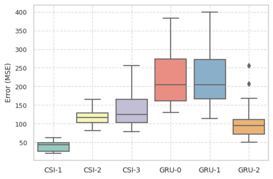
D.1 Effect on Choice of r
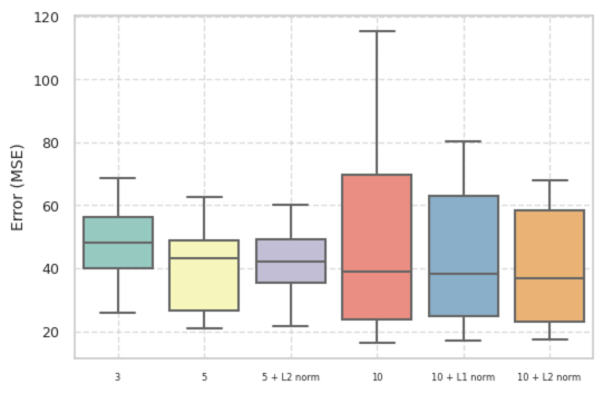
The effect of different is presented in Fig. 3, with being the ground truth parameter which data is generated. We have also plotted the performance of our method under and . We observed that when is smaller than the ground truth, the model tend to under-fit the data with a slight higher MSE error. When is bigger than the actual value, the MSE error can be further reduced but also at the same time results in very large variance. We also show that this can be mitigated with further regularization such as applying and terms during likelihood learning process.
The insight we drawn from this is that when apply our approach in real-world problems, we could potentially choose a higher without much concern about what an exact value should be. Using a large leads to higher variance but in general performs reasonable well compare with knowing the true (recall that here ). We also notice that applying regularization technique even when we know the right dimension of can be beneficial, leading to more stable performance (with lower variance), but does not change much of the mean estimate as shown in Fig. 3. This maybe partially caused by the gradient optimization process when training the deep neural network. Hence, we claim that the main price to be paid for a large choice of is that this makes data requirements stricter (such as the number of steps prior to the first intervention) in order to guarantee identification.
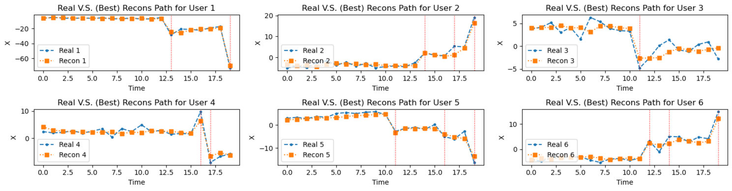
D.2 Additional Figures
Appendix E Uncertainty Quantification
For the sake of illustration, we generate another new dataset with a random seed of using the synthetic simulator, based on the following specifications: , , , , , , . We also generated two further datasets of , one for calibration and one for test.
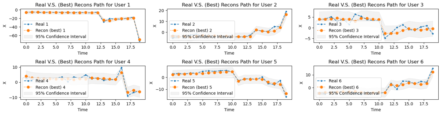
E.1 Plug-in Model-based Uncertainty Quantification
We first present the model based uncertainty quantification at level of , in Fig. 8. Given our conditional mean and homoscedastic error variance estimates from data, we can calculate predictive intervals as . For purely model based uncertainty quantification with plug-in parameter estimates, we do not need an additional calibration dataset, but it is an obviously problematic one as it does not take into account estimation error and sampling variability. The coverage rate is on the test dataset without further calibration.
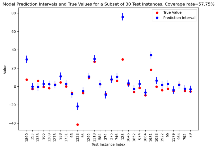
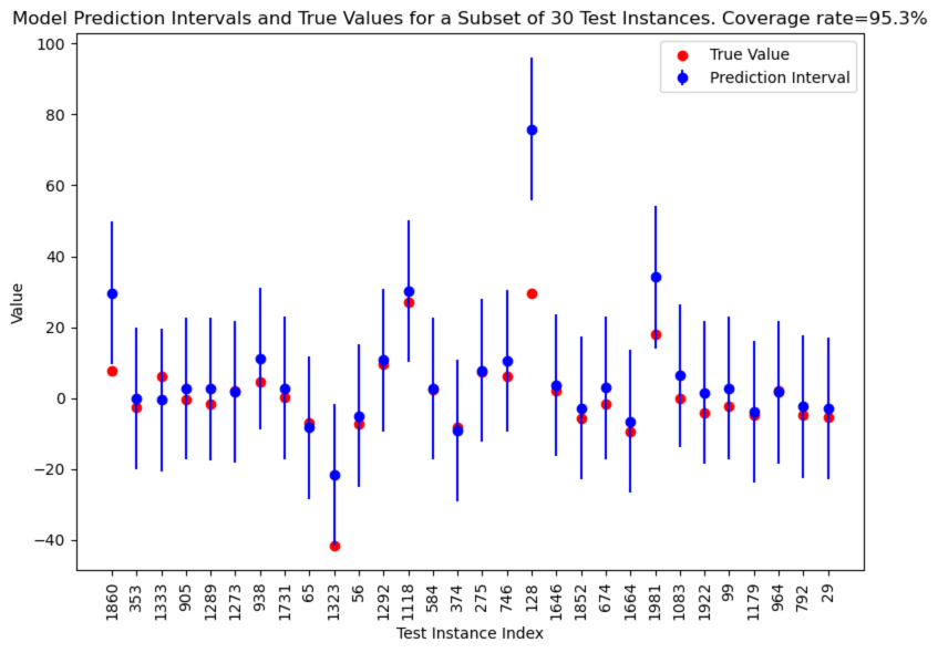
E.2 Conformal Prediction
We then present the model-free uncertainty quantification at level of (based on the Setup 1 in section 3.2), shown in Fig. 9. We use the absolute value over the predictive residual as our conformity score function, . We calibrate our model output based on the calibration dataset and then apply it on the test dataset. We obtained a coverage rate of . This is a significant improvement upon what we see in Fig. 8 and demonstrates the effectiveness of the conformal prediction approach.