Adversarial flows: A gradient flow characterization of adversarial attacks

Abstract

A popular method to perform adversarial attacks on neuronal networks is the so-called fast gradient sign method and its iterative variant. In this paper, we interpret this method as an explicit Euler discretization of a differential inclusion, where we also show convergence of the discretization to the associated gradient flow. To do so, we consider the concept of $p$-curves of maximal slope in the case $p=\infty$. We prove existence of $\infty$-curves of maximum slope and derive an alternative characterization via differential inclusions. Furthermore, we also consider Wasserstein gradient flows for potential energies, where we show that curves in the Wasserstein space can be characterized by a representing measure on the space of curves in the underlying Banach space, which fulfill the differential inclusion. The application of our theory to the finite-dimensional setting is twofold: On the one hand, we show that a whole class of normalized gradient descent methods (in particular signed gradient descent) converge, up to subsequences, to the flow, when sending the step size to zero. On the other hand, in the distributional setting, we show that the inner optimization task of adversarial training objective can be characterized via $\infty$-curves of maximum slope on an appropriate optimal transport space.

Keywords: adversarial attacks, adversarial training, metric gradient flows, Wasserstein gradient flows
AMS Subject Classification: 49Q20, 34A60, 68Q32, 65K15

1 Introduction

This paper considers gradient flows in metric spaces, following the seminal work by [2]. There, the authors introduce the concept of $p$-curves of maximal slope, with its origins dating back to [29]. This concept is further generalized in [79]. As for our main contribution, we study the less known limit case $p=\infty$ and adapt current theory to this setting. The main incentive for our work is the adversarial attack problem as introduced in [43, 90]. Here one considers a classification task, where a classifier $h:\mathcal{X}\to\mathcal{Y}$—typically parametrized as a neural network—is given an input $x\in\mathcal{X}$, which it correctly classifies as $y\in\mathcal{Y}$, where $\mathcal{Y}$ is assumed to be a subset of a finite dimensional vector space. The goal is to obtain a perturbed input $\tilde{x}\in\mathcal{X}$, the adversarial example, which is misclassified, while its difference to $x$ is “imperceptible”. In practice, the latter condition is enforced by requiring that $\tilde{x}$ has at most distance $\varepsilon$ to $x$ in an $\ell^{p}$ distance, where $\varepsilon>0$ is called the adversarial budget. Given some loss function $\ell:\mathcal{Y}\times\mathcal{Y}\to\mathbb{R}$, one then formulates the adversarial attack problem [43, 90],

$$\sup_{\tilde{x}\in\overline{B_{\varepsilon}}(x)}\ell(h(\tilde{x}),y).$$ (AdvAtt)

The above problem is also called an untargeted attack, since we are solely interested in the misclassification. This is opposed to targeted attacks, where one prescribes $y_{\text{target}}\in\mathcal{Y}$ and wants to obtain an adversarial example, s.t. $h(\tilde{x})=y_{\text{target}}$. This basically amounts to changing the loss function in AdvAtt, namely to $-\ell(\cdot,y_{\text{target}})$, without changing the inherent structure of the problem, which is why we do not consider it separately in the following. Methods for generating adversarial examples include first order attacks [63, 12, 71], momentum-variants [33], second order attacks [50] or even zero order attacks, not employing the gradient of the classifier [11, 48]. Especially for classifiers induced by neural networks, it was noticed that approximate maximizers of AdvAtt completely corrupt the classification performance, even for a very small budget $\varepsilon$. In order to obtain classifiers that are more robust against such attacks, the authors in [43] propose adversarial training (similarly derived in [58, 53]), where the standard empirical risk minimization is modified to

$$\inf_{h\in\mathcal{H}}\sum_{(x,y)\in\mathcal{T}}\sup_{\tilde{x}\in\overline{B_{\varepsilon}}(x)}\ell(h(\tilde{x}),y)$$ (AdvTrain)

for a training set $\mathcal{T}\subset\mathcal{X}\times\mathcal{Y}$ and a class of hypothesis $\mathcal{H}\subset\{h|h\,:\,\mathcal{X}\to\mathcal{Y}\}$. Since this requires solving AdvAtt for every data point $x$, the authors then propose an efficient one-step method, called Fast Gradient Sign Method (FGSM),

$$x_{\mathrm{FGS}}=x+\varepsilon\,\operatorname{sign}(\nabla_{x}\ell(h(x),y)).$$ (FGSM)

The motivation, as provided in [43], was to consider a linear model $x\mapsto\langle w,x\rangle$, with weights $w$. The maximum over the input $x$ constrained to the budget ball $\overline{B^{\infty}_{\varepsilon}}(x)$ is then attained in a corner of the hypercube, which validates the use of the sign. From a practical perspective, also for more complicated models, the sign operation ensures, that $x_{\mathrm{FGS}}\in\partial B_{\varepsilon}^{\infty}(x)$, i.e., $x_{\mathrm{FGS}}$ uses all the given budget in the $\ell^{\infty}$ distance, after just one update step. This adversarial training setup was similarly employed in [92, 85, 58, 80] and analyzed as regularization of the empirical risk in [18, 19]. For other strategies to obtain robust classifiers, we refer, e.g., to [20, 44, 52, 68]. In situations, where only the attack problem is of interest, multistep methods are feasible, which led to the iterative FGS method [54, 53]

$$x^{k+1}_{\mathrm{IFGS}}=\Pi_{\overline{B^{p}_{\varepsilon}}(x)}(x^{k}_{\mathrm{IFGS}}+\tau\,\operatorname{sign}(\nabla_{x}\ell(h(x^{k}_{\mathrm{IFGS}}),y))),$$ (IFGSM)

where $\tau>0$ now defines a step size and $\Pi_{\overline{B^{p}_{\varepsilon}}(x)}$ denotes the orthogonal $\ell^{p}$-projection to the $\varepsilon$-ball around the original image. Originally, the case $p=\infty$ was employed, where the projection is then a simple clipping operation. Other choices of $p$ are usually limited to $\{0,1,2\}$, which is also due to the computational effort of computing the projection (see [71] for $p=0$ and [34] for $p=1$). Signed gradient descent can also be interpreted as a form of normalized gradient descent in the $\ell^{\infty}$ topology as in [26], where our framework allows considering a general $\ell^{q}$ norm.

IFGSM g

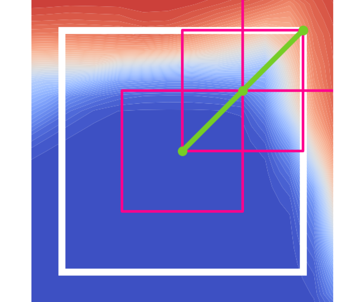
—- Minimizing Movement

(a) $\tau=0.2$

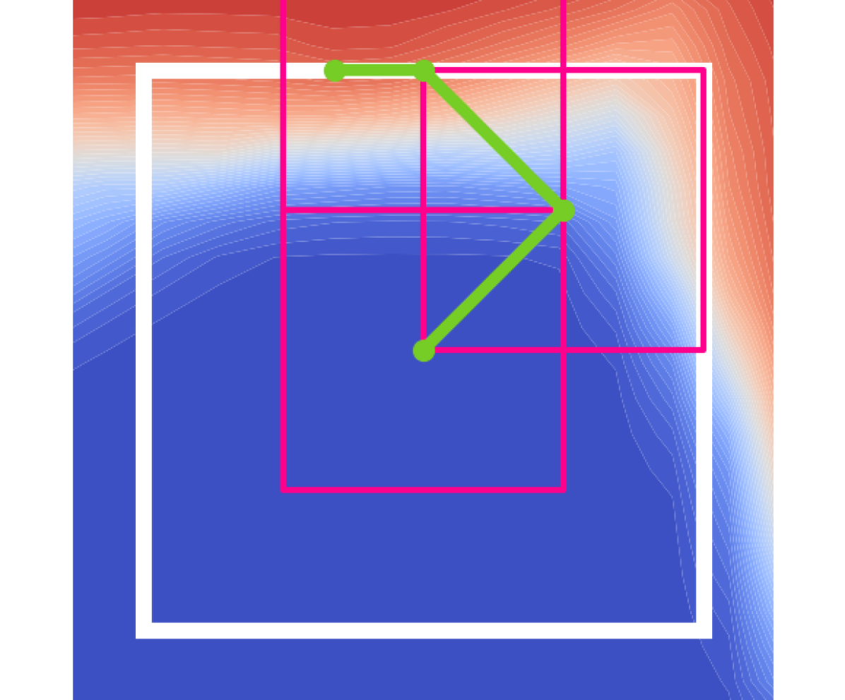
(b) $\tau=0.1$

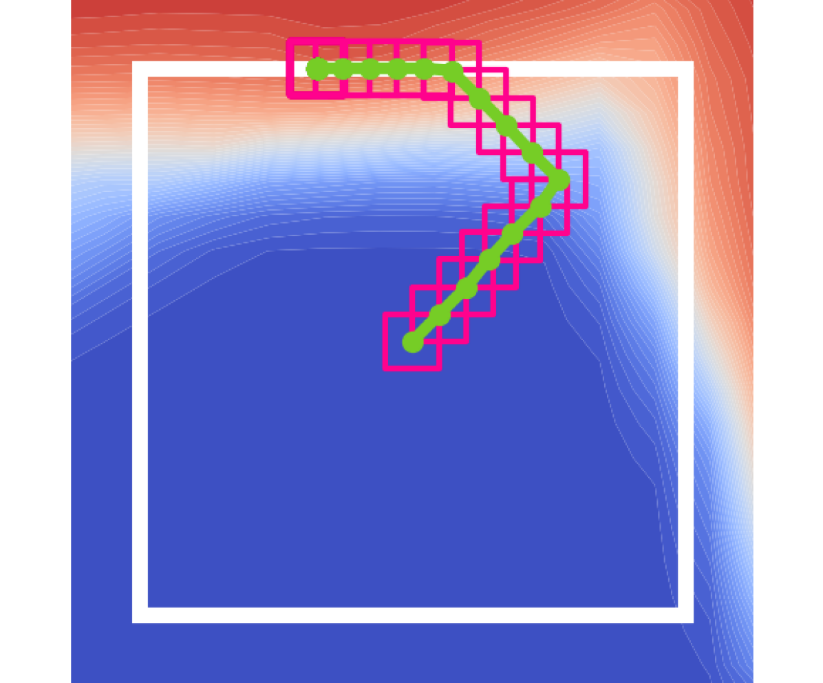
(c) $\tau=0.02$

(d) $\tau=0.001$

Figure 1: Behavior of IFGSM (top) and the minimizing movement scheme MinMove (bottom), for a binary classifier—parametrized as a neural network—on $\mathbb{R}^{2}$, a budget of $\varepsilon=0.2$, and $\tau\in\{0.2,0.1,0.02,0.001\}$. The white box indicates the maximal distance to the initial value, the pink boxes indicate the step size $\tau$ of the scheme. Details on this experiment can be found in appendix H.

Apart from the adversarial setting, signed gradient descent, without the projection step, is an established optimization algorithm itself, see e.g., [93, 62] for other applications. The idea of using signed gradients can also be found in the RPROP algorithm [74]. The convergence to minimizers of signed gradient descent and its variants was analyzed in [55, 5, 66, 25]. A slightly different kind of projected version, using linear constraints, was considered in [24], where the authors also considered a continuous time version, however, the results therein and the considered flow are not directly connected to our work here.

We consider the limit $\tau\to 0$ of signed gradient descent and the projected variant IFGSM, where we derive a gradient flow characterization, which is visualized in figure 1. In the Euclidean setting with a differentiable energy $\mathcal{E}:\mathbb{R}^{d}\to\mathbb{R}$ and $p\in(1,\infty)$, a differentiable curve $u:[0,T]\to\mathbb{R}^{d}$ is a $p$-curve of maximum slope, if it solves the $p$-gradient flow equation

$$\left(\left|u^{\prime}\right|(t)\right)^{p-2}\,u^{\prime}(t)=-\nabla\mathcal{E}(u(t)).$$

Here, we also refer to [15, 14] for a study of gradient-flow type equations in Hilbert spaces, for non-differentiable functionals. Following the approach in [29, 2, 30, 59], the above equation is equivalent to

$$\frac{d}{dt}(\mathcal{E}\circ u)\leq-\frac{1}{p}\left|u^{\prime}\right|^{p}-\frac{1}{q}\left|\nabla\mathcal{E}(u)\right|^{q},$$

where $1/p+1/q=1$. The strength of this approach, is that all derivatives in the above inequality, have meaningful generalizations to the metric space setting, which we repeat in the next section. Motivated by signed gradient descent, in this paper we draw the connection to the case $p=\infty$. In the Euclidean setting, with a differentiable functional $\mathcal{E}$, the energy dissipation inequality we derive for $p=\infty$, reads

$$\left|u^{\prime}\right| \leq 1,$$

$$\frac{d}{dt}(\mathcal{E}\circ u) \leq-\left|\nabla\mathcal{E}(u)\right|.$$

Intuitively, a $\infty$-curve of maximal slope minimizes the energy $\mathcal{E}$ as fast as possible under the restriction that its velocity $\left|u^{\prime}\right|$ is bounded by $1$. Like in [2], our results consider general metric spaces, Banach spaces and Wasserstein spaces, which are further detailed in the following sections. Typically, curves of maximum slope can be approximated via a minimizing movement scheme, which in our case translates to

$$x^{k+1}_{\tau}\in\operatorname*{arg\,min}_{x\in\mathcal{X}}\{\mathcal{E}(x)\,:\,\left\|x-x^{k}_{\tau}\right\|\leq\tau\},$$

where $x^{0}_{\tau}=x^{0}$ is a given initial value. A main insight, explored in section 5, is that under certain assumption FGSM and IFGSM fulfill this scheme, if we replace the energy by a semi-implicit version.

A further aspect, is the characterization of adversarial attacks in the distributional setting, where the sum is replaced by an integral over the data distribution $\mu$. Interchanging the integral and the supremum (see corollary 5.7), yields the characterization of adversarial training AdvTrain as a distributionally robust optimization (DRO) problem,

$$\inf_{h\in\mathcal{H}}\sup_{\tilde{\mu}:D(\mu,\tilde{\mu})\leq\varepsilon}\int\ell(h(x),y)d\tilde{\mu}(x,y),$$ (DRO)

where $D$ denotes a distance on the space of distributions. This formulation of adversarial training was the subjects of many studies in recent years, see, e.g., [18, 94, 19, 21, 22]. Typically, the distance $D$ is chosen an optimal transport distance,

$$D(\mu,\tilde{\mu})\coloneqq\inf_{\gamma\in\Gamma(\mu,\tilde{\mu})}\int_{\gamma}c((x,y),(\tilde{x},\tilde{y}))^{2}d\gamma,$$

with $\gamma(\mu,\tilde{\mu})$ denoting the set of all couplings and the cost

$$c((x,y),(\tilde{x},\tilde{y}))\coloneqq\begin{cases}\|x-\tilde{x}\|_{2}&\text{if }y=\tilde{y},\\ +\infty&\text{if }y\neq\tilde{y}.\end{cases}$$ (1.1)

The goal here is then to derive a characterization of curves $\mu:[0,T]\to\mathcal{W}_{p}$, where $\mathcal{W}_{p}$ denotes the $p$-Wasserstein space. In this regard, we mention the related work [94], where the authors proposed to solve the inner optimization problem

$$\sup_{\tilde{\mu}:D(\mu,\tilde{\mu})\leq\varepsilon}\int\ell(h(x),y)d\tilde{\mu}(x,y)$$

by disintegrating the data distribution $d\mu(x,y)=d\mu_{y}(x)d\nu(y)$ (see appendix E), and calculating for $\nu$-a.e. $y\in\mathcal{Y}$ the corresponding $2$-gradient flow in $\mathcal{W}_{2}$ with initial condition $\mu_{y}^{0}$. As shown in [2] solving this gradient flow is equivalent to solving the partial differential equation

$$\begin{aligned} \partial_{t}(\mu_{y})_{t}=\nabla\cdot((\mu_{y})_{t}\nabla_{x}\ell(h(x),y))&\quad\text{on }(0,T)\\ (\mu_{y})_{0}=\mu_{y}^{0},&\end{aligned}$$ (1.2)

which is to be understood in the distributional sense. The authors in [94] then approximate a maximizer by $d\tilde{\mu}(x,y)\approx d(\mu_{y})_{T}(x)d\nu(y)$, where $T$ has to be chosen small enough such that the approximation is still within the $\varepsilon$ ball around $\mu$.

In the following, we first provide the necessary notions for gradient flows in metric spaces and then proceed to discuss the main contributions and the outline of this paper.

1.1 Setup

We give a brief recap on classical notation and preliminaries on evolution in metric spaces. More details can be found in [2, 61]. In the following, we denote by $(\mathcal{S},d)$ a complete metric space, while $\mathcal{X}$ denotes a Banach space. We consider a proper functional $\mathcal{E}:\mathcal{S}\rightarrow(-\infty,+\infty]$, i.e., the effective domain $\operatorname{dom}(\mathcal{E})\coloneqq\{x\in\mathcal{S}\,:\,\mathcal{E}(x)<\infty\}$ is assumed to be nonempty. Throughout this paper we denote by

$$B_{\tau}(x):=\{\tilde{x}\in\mathcal{S}\,:\,d(x,\tilde{x})<\tau\},\qquad\overline{B_{\tau}}(x):=\{\tilde{x}\in\mathcal{S}:d(x,\tilde{x})\leq\tau\}$$

the ball and its closed variant, induced by the given metric $d$, where we employ the abbreviation $B_{\tau}(0)=B_{\tau}$. In the finite dimensional case, we write $B^{p}_{\tau}$ to denote the ball induced by the $\ell^{p}$ norm on $\mathbb{R}^{d}$. Note, that there is a notation conflict with $d$ denoting both the distance and the dimension of the finite-dimensional space $\mathbb{R}^{d}$. However, the concrete meaning is always clear from the context.

Metric derivative

We consider curves $u:[0,T]\rightarrow\mathcal{S}$ with $T>0$ for which we want to have a notion of velocity. For this sake, we need a generalization of the absolute value of the derivatives, which is provided by the metric derivative as introduced by [1]. Here, one usually considers $p$-absolutely continuous curves [2], i.e., for $p\in[1,\infty]$ there exists $m\in L^{p}(0,T)$ such that

$$d(u(t),u(s))\leq\int_{s}^{t}m(r)dr$$ (1.3)

for all $0\leq s<t\leq T$. The set of all $p$-absolutely continuous curves is denoted by $AC^{p}(0,T;\mathcal{S})$. We are especially interested in the case $p=\infty$, where the condition in equation 1.3 is equivalent to the Lipschitzness of the curve, i.e., the existence of a constant $L\geq 0$ such that

$$d(u(t),u(s))\leq L\ (t-s)$$

for all $0\leq s<t\leq T$. For the special case $p=\infty$, we have the following result as a special case of [2, Theorem 1.1.2].

Lemma 1.1 (Metric Derivative).

Let $u:[0,T]\rightarrow\mathcal{S}$ be a Lipschitz curve with Lipschitz constant $L$, then the limit

$$|u^{\prime}|(t)\coloneqq\lim_{s\rightarrow t}\frac{d(u(s),u(t))}{|s-t|}$$

exists for a.e. $t\in[0,T]$ and is referred to as the metric derivative. Moreover, the function $t\mapsto|u^{\prime}|(t)$ belongs to $L^{\infty}(0,T)$ with $\||u^{\prime}|\|_{L^{\infty}(0,T)}\leq L$, and

$$d(u(s),u(t))\leq\int_{s}^{t}|u^{\prime}|(r)dr\quad\ \text{for all }0\leq s\leq t\leq T.$$

Remark 1.2.

The metric derivative $|u^{\prime}|$ is actually minimal in the sense that for every $m$ satisfying 1.3,

$$|u^{\prime}|(t)\leq m(t)\quad\text{for a.e. }t\in(0,T).$$

Remark 1.3.

If $\mathcal{S}=\mathcal{X}$ is a Banach space and satisfies the Radon–Nikodým property (c.f. [81, p. 106]), e.g., if it is reflexive, then $u\in AC^{p}(0,T;\mathcal{X})$ if and only if

• $u$ is differentiable a.e. on $(0,T)$

• $u^{\prime}(t)\in L^{p}(0,T;\mathcal{X})$

• $u(t)-u(s)=\int_{s}^{t}u^{\prime}(t)dr$ for $0\leq s\leq t\leq T$.

Upper gradients

We consider upper gradients as a generalization of the absolute value of the gradient in the metric setting. Namely, we employ the following definitions from [2, Definition 1.2.1] and [2, Definition 1.2.2].

Definition 1.4.

A function $g:\mathcal{S}\to[0,+\infty]$ is called a strong upper gradient for $\mathcal{E}$, if for every absolutely continuous curve $u:[0,T]\to\mathcal{S}$ the function $g\circ u$ is Borel and

$$|\mathcal{E}(u(t))-\mathcal{E}(u(s))|\leq\int_{s}^{t}g(u(r))|u^{\prime}|(r)dr\quad\forall\ 0\leq s\leq t\leq T$$

If $(g\circ u)\,|u^{\prime}|\in L^{1}(0,T)$ then $\mathcal{E}\circ u$ is absolutely continuous and

$$|(\mathcal{E}\circ u)^{\prime}(t)|\leq g(u(t))|u^{\prime}|(t)\quad\text{for a.e. }t\in(0,T).$$ (1.4)

Definition 1.5.

A function $g:\mathcal{S}\to[0,+\infty]$ is called a weak upper gradient for $\mathcal{E}$, if for every absolutely continuous curve $u:[0,T]\to\mathcal{S}$ that fulfills

1. $(g\circ u)\ \left|u^{\prime}\right|\in L^{1}(0,T)$,

2. $\mathcal{E}\circ u$ is a.e. in $(0,T)$ equal to a function $\psi:(0,T)\to\mathbb{R}$ with bounded variation,

it follows that

$$\left|\psi^{\prime}\right|\leq(g\circ u)\ \left|u^{\prime}\right|\text{ a.e. in }(0,T).$$

Remark 1.6.

We note that for a function $\psi$ with bounded variation, i.e.,

$$\sup\left\{\sum_{i=0}^{N-1}\left|\psi(t_{i+1})-\psi(t_{i})\right|\,:\,0=t_{0}<\ldots<t_{N}=T\right\}<\infty,$$

we have that the derivative $\psi^{\prime}$ exists a.e. in the interval $(0,T)$, see [82, Theorem 9.6, Chapter IV].

Remark 1.7.

Admissible curves $u$ in the above definition fulfill that $u^{-1}(\mathcal{S}\setminus\operatorname{dom}(\mathcal{E}))$ is a null set, because of (ii). Therefore, the behavior of $g$ outside of $\operatorname{dom}(\mathcal{E})$ is negligible.

Metric slope

We now consider the metric slope, as defined in [29], as a special realization of a weak upper gradient. Intuitively, the slope gives the value of the maximal descent at a point $u$ at a infinitesimal small distance.

Definition 1.8.

For a proper functional $\mathcal{E}:\mathcal{S}\rightarrow(-\infty,+\infty]$, the local slope of $\mathcal{E}$ at $x\in\operatorname{dom}(\mathcal{E})$ is defined as

$$|\partial\mathcal{E}|(x)\coloneqq\limsup_{z\rightarrow x}\frac{(\mathcal{E}(x)-\mathcal{E}(z))^{+}}{d(x,z)}.$$

The definition of the slope does in fact yield an upper gradient, which is provided by the following statement from [2].

Theorem 1.9 ([2, Theorem 1.2.5]).

Let $\mathcal{E}$ be a proper functional, then the function $\left|\partial\mathcal{E}\right|$ is a weak upper gradient.

Curves of maximal slope

Curves of maximal slope were introduced in [29] and are a possible generalization of a gradient evolution in metric spaces. They are usually formulated for the case $p\in(1,\infty)$ as follows, see, e.g., [2].

Definition 1.10 ($p$-Curves of maximal slope).

For $p\in(1,\infty)$ we say that an absolutely continuous curve $u:[0,T]\to\mathcal{S}$ is a $p$-curve of maximal slope, for the functional $\mathcal{E}$ with respect to an upper gradient $g$, if $\mathcal{E}\circ u$ is a.e. equal to a non-increasing map $\psi$ and

$$\psi^{\prime}(t)\leq-\frac{1}{p}\left|u^{\prime}\right|^{p}(t)-\frac{1}{q}g^{q}(u(t))$$ (1.5)

for almost every $t\in(0,T)$ and $1=\frac{1}{p}+\frac{1}{q}$.

For $p\in(1,\infty)$, the existence of such curves is provided, see for example [2].

1.2 Main results

In section 2, we consider the notion of $p$-curves of maximal slope to the case $p=\infty$, for Lipschitz curves $u$. As hinted in the introduction, in the limit $p\to\infty$ of definition 1.10, we replace 1.5 by the following condition,

$$\left|u^{\prime}\right|(t) \leq 1,$$

$$\quad\psi^{\prime}(t) \leq-g(u(t)).$$

Such curves are then called $\infty$-curves of maximal slope, for which we prove the following existence statement. The concrete assumptions are provided in section 2.

Theorem (Existence).

Under the assumptions specified in section 2, for every $\mathcal{E}:\mathcal{S}\to(-\infty,+\infty]$ and for every $x^{0}\in dom(\mathcal{E})$, there exists a Lipschitz curve $u:[0,T]\to\mathcal{S}$ with $u(0)=x^{0}$, which is a $\infty$-curve of maximum slope with respect to the weak upper gradient $|\partial\mathcal{E}|$.

We note that this result can also be obtained as a corollary of a more general existence result in [79]. Therein, the authors prove existence of curves of maximal slope fulfilling

$$\psi^{\prime}(t)\leq-f^{*}(g(u(t)))-f(\left|u^{\prime}\right|(t))$$

for a convex and lower semicontinuous function $f:[0,\infty)\to[0,\infty)$. When choosing $f=\chi_{[0,1]}$, we recover our notion of $\infty$-curves of maximal slope. Although, the existence proof in section 2 employs similar concepts, we choose to include it here. On the one hand, the treatment of this specific case allows for certain arguments, that are not directly possible in the general case. On the other hand, this section forms the formation for the rest of the paper, which can not directly be deduced from [79].

In section 3, we consider the specific case of $\infty$-curves of maximal slope in a Banach space $\mathcal{X}$, when the Energy $\mathcal{E}$ is a $C^{1}$ convex perturbation. We derive an equivalent characterization of $\infty$-curves of maximal slope via a differential inclusion. We note that this differential inclusion was not considered in [79].

Theorem (Differential inclusion).

Let $\mathcal{E}:\mathcal{X}\rightarrow(-\infty,+\infty]$ satisfy 3.6 and $u:[0,1]\rightarrow\mathcal{X}$ be an a.e. differentiable Lipschitz curve. Let further $\mathcal{E}\circ u$ be a.e. equal to a non-increasing function $\psi$, then the following are equivalent:

1. $|u^{\prime}|(t)\leq 1$ and $\psi^{\prime}(t)\leq-|\partial\mathcal{E}|(u(t))$ for a.e. $t\in[0,1]$,

2. $u^{\prime}(t)\subset\partial\|\cdot\|_{*}(-\xi)\quad\forall\xi\in\partial^{\circ}\mathcal{E}(u(t))\not=\emptyset,$ for a.e. $t\in[0,1],$

where $\partial^{\circ}\mathcal{E}(u(t))$ denotes those elements of minimal of $\partial\mathcal{E}(u(t))$.

Regarding the application to IFGSM, we consider an alternative minimizing movement scheme, by employing a semi-implicit energy

$$\mathcal{E}^{\mathrm{sl}}(x;z)\coloneqq\mathcal{E}^{\mathrm{d}}(z)+\langle D\mathcal{E}^{\mathrm{d}}(z),x-z\rangle+\mathcal{E}^{\mathrm{c}}(x).$$

In the case of $p=2$ we refer to [38, 89] for other works that also consider approximate minimizing movement schemes. This semi-implicit scheme is useful, since in the finite dimensional adversarial setting it allows us to choose $-\ell(h(\cdot),y)$ as the differentiable part, and additionally to incorporate the budget constraint via the indicator function $\chi_{\overline{B_{\varepsilon}}(x)}$. We can show that up to a subsequence, this scheme also convergences to a $\infty$-curve of maximum slope, in the topology $\sigma$ as specified in assumption 1.a.

Theorem.

Under the assumptions specified in section 3, there exists a $\infty$-curve of maximal slope $u$ and a subsequence of $\tau_{n}=T/n$ such that

$$\bar{x}_{\mathrm{sl},\tau_{n}}(t)\stackrel{{\scriptstyle\sigma}}{{\rightharpoonup}}u(t)\text{ as }n\rightarrow\infty\quad\forall t\in[0,T].$$

In order to better understand the connection between the differential inclusion and IFGSM, we want to highlight, that $\infty$-curves of maximum slope yield a general concept, which is not directly tied to signed gradient descent and the choice of the projection. The intuition behind $\infty$-curves is rather connected to employing normalized gradient descent (NGD) [26]. Choosing $(\mathbb{R}^{d},\left\|\cdot\right\|_{p})$ as the underlying Banach space, in section 5 we see that for $1/p+1/q=1$ the following iteration fulfills the semi-implicit minimizing movement scheme,

$$x^{k+1}=x^{k}+\tau\ \operatorname{sign}(\nabla_{x}\mathcal{E}(x^{k}))\cdot\left(\frac{\left|\nabla_{x}\mathcal{E}(x^{k})\right|}{\left\|\nabla_{x}\mathcal{E}(x^{k})\right\|_{q}}\right)^{q-1},$$

where the absolute value and multiplication is understood entrywise. Choosing $p=2$ or $p=\infty$ recovers the notion of NGD as in [26]. In the setting of adversarial attacks, this means, that we want to ensure that the iterates exploit the maximum allowed budget (locally on $\overline{B_{\tau}}(x^{k})$ ball) in each step. This was similarly observed in [33]. As long as the iterates stay within the given budget $\varepsilon$, this then yields that IFGSM is an explicit solution to the semi-implicit scheme and therefore converge to $\infty$-curves of maximum slope. In the more interesting case, where the projection has an effect, we need to ensure that minimizing on $\overline{B_{\tau}^{p}}(x)$ and then projecting to $\overline{B_{\varepsilon}^{p}}(x^{0})$ is equivalent to directly minimizing on $\overline{B_{\varepsilon}^{p}}(x^{0})\cap\overline{B_{\tau}^{p}}(x)$. We show this property for the case $p=\infty$. Employing the convergence result for the semi-implicit minimizing movement scheme, then yields the convergence up to subsequences of IFGSM, employing the $\ell^{\infty}$ norm.

Theorem.

Under the assumptions specified in section 5, for $T>0$, there exists a $\infty$-curve of maximal slope $u:[0,T]\to\mathbb{R}^{d}$, with respect to $\mathcal{E}$, and a subsequence of $\tau_{n}:=T/n$ such that

$$\left\|x^{\lceil t/\tau_{n_{i}}\rceil}_{\mathrm{IFGS},\tau_{n_{i}}}-u(t)\right\|\xrightarrow{i\to\infty}0\qquad\text{ for all }t\in[0,T].$$

In section 4 we consider potential energies

$$\mathcal{E}:W_{\infty}(\mathcal{X})\ni\mu\mapsto\int E(x)d\mu(x),$$

where in our context, the potential $E:\mathcal{X}\rightarrow(-\infty,+\infty]$ has the form $E(x)=-\ell(h(x),y)$. The basis for our main result in this section is given by [57, Thm. 3.1], which is repeated as theorem 4.7 in this paper. Namely, we characterize absolutely continuous curves $\mu\in\mathrm{AC}^{p}(0,T;W_{p})$ by a measure $\eta$ on the space of curves $u:[0,T]\to\mathcal{X}$, which is concentrated on $\mathrm{AC}^{p}(0,T;\mathcal{X}$). Using this representation, we show that being a $\infty$-curve of maximum slope in the Wasserstein space is equivalent to the differential inclusion on the underlying Banach space, for $\eta$-a.e. curve.

Theorem.

Under the assumptions specified in theorem 4.19, for a curve $\mu\in\mathrm{AC}^{\infty}(0,T,W_{\infty})$ with $\eta$ from theorem 4.7, the following statements are equivalent:

1. The curve $\mu$ is $\infty$-curve of maximal slope w.r.t. to the weak upper gradient $\left|\partial\mathcal{E}\right|$.

2. For $\eta$-a.e. curve $u\in C(0,T;\mathcal{X})$ it holds, that $E\circ u$ is for a.e. $t\in(0,T)$ equal to a non-increasing map $\psi_{u}$ and

   $$u^{\prime}(t)\subset\partial\|\cdot\|_{*}(-\xi)\quad\forall\xi\in\partial^{\circ}E(u(t))\not=\emptyset,\quad\text{for a.e. }t\in(0,T).$$

When applying this result to adversarial training, we slightly deviate from the Wasserstein setting, by choosing the extended distance in 1.1 and the associated transported distance, in order to prohibit mass transport into the label direction. However, we can adjust the arguments in section 4 to derive an analogous result for the energy $\mathcal{G}(\mu)\coloneqq\int-\ell(h(x),y)d\mu(x,y)$, which we state in theorem 5.9. Here, we only enforce the budget constraint, by setting the end time of the flow to $T=\varepsilon$.

1.3 Outline

The paper is organized as follows: In section 2, we start by introducing $\infty$-curves of maximal slope, as the limit case of $p$-curves of maximal slope. section 2.3 then provides an existence result for those curves in a general metric setting. The underlying assumptions for its proof are stated in section 2.1.

In section 3, we consider $\infty$-curves of maximal slope when the underlying metric space is a Banach space. section 3.1 introduces $C^{1}$-perturbations of convex functions as a convenient class of functionals, that covers most of the energies we consider in this paper. In section 3.2, we derive equivalent characterizations of $\infty$-curves of maximal slope via a doubly nonlinear differential inclusion. This section is concluded by investigating first order approximation techniques of those differential inclusions in section 3.3.

section 4 is devoted to $\infty$-curves of maximal slope, when the underlying space is the $\infty$-Wasserstein space. For potential energies we give an equivalent characterization of $\infty$-curves of maximal slope via a probability measures $\eta$ on the space $C(0,T;\mathcal{X})$ which is concentrated on $\infty$-curves of maximal slope on the underlying Banach space $\mathcal{X}$. From $\eta$, we can then derive a corresponding continuity equation for those curves of maximal slope.

In section 5, we discuss the application of differential inclusions derived in section 3 to generate adversarial examples. We show that the popular fast gradient sign method (FGSM) and its iterative variant (IFGSM) are simple first order approximations of $\infty$-curves of maximal slope. In section 5.2, we rewrite adversarial training as a distributional robust optimization problem and discuss the usage of $\infty$-curve in the corresponding probability space, to generate distributional adversaries.

2 Infinity Flows in metric spaces

In this section, we generalize the notion of $p$-curves of maximal slope to the case $p=\infty$. We consider the convex function $f(x)=\frac{1}{p}|x|^{p}$, which allows us to express the energy dissipation inequality 1.5 in definition 1.10 as follows,

$$\psi^{\prime}(t)\leq-f(|u^{\prime}|(t))-f^{*}(g(u(t))),$$ (2.1)

where $f^{*}(x^{*})=\frac{1}{q}|x^{*}|^{q}$ denotes the convex conjugate of $f$. Considering the above inequality for arbitrary convex functions $f$ leads to the general framework as introduced in [79]. For our setting, we consider the characteristic function, which is obtained as the following pointwise limit,

$$\frac{1}{p}\left|x\right|^{p}\xrightarrow[]{p\to\infty}\chi_{[-1,1]}(x)=\begin{cases}0\text{ if }|x|\leq 1,\\ +\infty\text{ else},\end{cases}$$

where $\chi_{[-1,1]}$ is a convex function with conjugate $\chi_{[-1,1]}^{*}(x^{*})=x^{*}$. Using $f=\chi_{[-1,1]}$ in equation 2.1 forces the curves of maximal slope to obey $\left|u^{\prime}\right|\leq 1$ almost everywhere and the energy dissipation inequality becomes

$$\psi^{\prime}(t)\leq-g\circ u(t),$$

which motivates the following definition.

Definition 2.1 ($\infty$-Curve of maximal slope).

We say an absolutely continuous curve $u:[0,T]\rightarrow\mathcal{S}$ is an $\infty$-curve of maximal slope for the functional $\mathcal{E}$ with respect to an upper gradient $g$, if $\mathcal{E}\circ u$ is a.e. equal to a non-increasing map $\psi$ and

$$\begin{split}|u^{\prime}|(t)&\leq 1,\\ \quad\psi^{\prime}(t)&\leq-g(u(t)),\end{split}$$ (InfFlow)

holds for a.e. $t\in(0,T)$.

Remark 2.2.

We note that the condition $\left|u^{\prime}\right|\leq 1$ a.e., implies that $u$ is a Lipschitz curve with Lipschitz constant $1$, see lemma 1.1.

Example 1.

As an easy example, let us look at the quadratic energy $\mathcal{E}:x\mapsto\frac{1}{2}x^{2}$ on the space $(\mathcal{S},d)=(\mathbb{R},|\cdot-\cdot|)$. Its metric slope and thus weak upper gradient is given by $\left|\partial\mathcal{E}\right|(x)=\left|\frac{d}{dx}\mathcal{E}\right|(x)=\left|x\right|$. We choose $x^{0}=1$ as the starting point, then the corresponding $\infty$-curve of maximal slope is

$$u(t)=\begin{cases}1-t&\text{if }0\leq t\leq 1,\\ 0&\text{if }t>1\end{cases}.$$

We directly observe that $\left|u^{\prime}\right|\leq 1$ and

$$\mathcal{E}(u(t))=\begin{cases}\frac{1}{2}(1-t)^{2}&\text{if }0\leq t\leq 1,\\ 0&\text{if }t>1,\end{cases}$$

is a non-increasing map with

$$\frac{d}{dt}\mathcal{E}(u(t))=\begin{cases}t-1&\text{if }0\leq t<1,\\ 0&\text{if }t>1,\end{cases}=-\left|u(t)\right|=-\left|\partial\mathcal{E}\right|(u(t)),$$

and therefore the conditions InfFlow are fulfilled. Here we can already observe a typical behavior of $\infty$-curves of maximal slope. They have a constant velocity of $1$ until they hit a local minimum where they stop abruptly.

The rest of this section is devoted to an existence proof for $\infty$-curves of maximal slope.

2.1 Assumptions for existence

Here, we state the assumptions needed for the proof of existence. Approximations of curves of maximal slope are constructed via a minimizing movement scheme. To guarantee convergence of those approximations, a form of relative compactness is essential. This is guarantied by assumption 1.b. Furthermore, relative compactness with respect to the topology induced by the metric $d(\cdot,\cdot)$ may not be given. However, relative compactness with respect to a weaker topology $\sigma$ is sufficient, as long as it is compatible with the topology induced by the metric $d(\cdot,\cdot)$, assumption 1.a. These assumptions were also employed in [2].

Assumption 1.a (Weak topology).

In addition to the metric topology, $(\mathcal{S},d)$ is assumed to be endowed with a Hausdorff topology $\sigma$. We assume that $\sigma$ is compatible with the metric $d$, in the sense that $\sigma$ is weaker than the topology induced by $d$ and $d$ is sequentially $\sigma$-lower semicontinuous, i.e., $\displaystyle(x^{n},z^{n})\stackrel{{\scriptstyle\sigma}}{{\rightharpoonup}}(x,z)\Longrightarrow\liminf_{n\rightarrow\infty}d(x^{n},z^{n})\geq d(x,z).$

Assumption 1.b (Relative compactness).

Every $d$-bounded set contained in sublevels of $\mathcal{E}$ is relatively $\sigma$-sequentially compact, i.e., $$\displaystyle\text{if}\quad\{x^{n}\}_{n\in\mathbb{N}}\subset\mathcal{S}\quad\text{with}\quad\sup_{n\in\mathbb{N}}\mathcal{E}(x^{n})<+\infty,\quad\sup_{n,m}d(x^{n},x^{m})<+\infty,$$ $$\displaystyle\text{then }\left(x^{n}\right)_{n\in\mathbb{N}}\text{ admits a }\sigma\text{-convergent subsequence.}$$

assumptions 2.a and 2.b ensure continuity of energy functional and lower semicontinuity of its metric slope. These regularity assumptions are required for the energy dissipation inequality during the limiting process in the proof of theorem 2.11.

Assumption 2.a (Continuity).

We assume $\sigma$-sequential continuity of $\mathcal{E}$ for particular sequences: $\displaystyle\left.\begin{aligned} \sup_{n\in\mathbb{N}}\left\{d(x_{n},x_{0}),\mathcal{E}(x_{n})\right\}<\infty,\\ x_{n}\stackrel{{\scriptstyle\sigma}}{{\rightharpoonup}}x\end{aligned}\right\}\Longrightarrow\mathcal{E}(x_{n})\rightarrow\mathcal{E}(x).$ (2.2)

Assumption 2.b (Lower semicontinuity of Slope).

In addition, we ask that $|\partial\mathcal{E}|$ is sequentially $\sigma$-lower semicontinuous on $d$-bounded sublevels of $\mathcal{E}$.

Remark 2.3.

The proof of existence is possible with a wide variety of regularity assumptions on the energy $\mathcal{E}$, which can be tailored to a variety of different situations. For example, if the sequentially $\sigma$-lowers semicontinuous envelope of $|\partial\mathcal{E}|$

$$|\partial^{-}\mathcal{E}|\coloneqq\left\{\liminf_{n\rightarrow\infty}|\partial\mathcal{E}|(x_{n})\,:\,x_{n}\stackrel{{\scriptstyle\sigma}}{{\rightharpoonup}}x,\sup_{n}{d(x_{n},x),\mathcal{E}(x_{n})}<+\infty\right\}$$

is a weak upper gradient, one can drop assumption 2.b and instead prove existence of curves of maximal slope with respect to $|\partial^{-}\mathcal{E}|$. Further, if $|\partial\mathcal{E}|$ (or $|\partial^{-}\mathcal{E}|$ respectively) is a strong upper gradient (compare [2, Theorem 2.3.3]) then assumption 2.a can be relaxed to lower semicontinuity and the energy dissipation inequality 2.1 becomes an equality.

Remark 2.4.

When $u(t)\in\operatorname{dom}\mathcal{E}$ for all $t\in[0,T]$, then due to assumption 2.a, the concatenation $\mathcal{E}\circ u$ is continuous and obtains its minimum $(\mathcal{E}\circ u)_{\min}$ and maximum $(\mathcal{E}\circ u)_{\max}$. In particular, the maximum and minimum have to be finite. By lemma E.1 we know $\psi(t)\in[(\mathcal{E}\circ u)_{\min},(\mathcal{E}\circ u)_{\max}]$ for all $t\in(0,T)$. Now we can simply set $\psi(0)\coloneqq(\mathcal{E}\circ u)_{\max}$ and $\psi(T)\coloneqq(\mathcal{E}\circ u)_{\min}$, without affecting $\psi^{\prime}(t)$ a.e. on $(0,T)$. So without loss of generality we can assume that $\psi$ is a non-increasing map with $\psi(0)=(\mathcal{E}\circ u)_{\max}$ and $\psi(T)=(\mathcal{E}\circ u)_{\min}$ and therefore it is of bounded variation.

Remark 2.5.

(Dissipation equality) If $g$ is a strong upper gradient of $\mathcal{E}$ and $u(t)\in\operatorname{dom}\mathcal{E}$ for all $t\in[0,T]$, then by definition 1.4 and InfFlow

$$|\mathcal{E}(u(t))-\mathcal{E}(u(s))|\leq\int_{s}^{t}g(u(r))|u^{\prime}|(r)dr\leq\int_{s}^{t}g(u(r))dr\leq\int_{s}^{t}-\psi^{\prime}(r)dr<+\infty.$$

This integral is finite due to the fact that $\psi$ is a function of bounded variation and thus $\mathcal{E}\circ u$ is absolutely continuous. This in particular implies $\psi(t)=(\mathcal{E}\circ u)(t)$ for all $t\in(0,T)$ (see lemma E.2) and thus $\psi^{\prime}(t)=(\mathcal{E}\circ u)^{\prime}(t)$ for a.e. $t\in(0,T)$. Furthermore, remark 1.3 implies

$$\mathcal{E}(u(t))-\mathcal{E}(u(s))=\int_{s}^{t}(\mathcal{E}\circ u)^{\prime}(r)dr\quad\text{for }0\leq s\leq t\leq T$$

and we can estimate

$$\mathcal{E}(u(t))-\mathcal{E}(u(s))=\int_{s}^{t}(\mathcal{E}\circ u)^{\prime}(r)dr\leq\int_{s}^{t}-g(u(r))dr\quad\text{for }0\leq s\leq t\leq T$$

and on the other hand using 1.4, we obtain

$$\mathcal{E}(u(t))-\mathcal{E}(u(s)) =\int_{s}^{t}(\mathcal{E}\circ u)^{\prime}(r)dr\geq\int_{s}^{t}-|(\mathcal{E}\circ u)^{\prime}(r)|dr$$

$$\geq\int_{s}^{t}-g(u(r))|u^{\prime}|(r)dr\geq\int_{s}^{t}-g(u(r))dr$$

for $0\leq s\leq t\leq T$. Therefore, the energy dissipation equality

$$\mathcal{E}(u(t))-\mathcal{E}(u(s))=\int_{s}^{t}-g(u(r))dr$$

holds for every $0\leq s\leq t\leq T$ .

2.2 Minimizing movement for $p=\infty$

The minimizing movement scheme is an implicit time discretization of curves of maximal slope. The existence of curves of maximal slope is proven by sending the discrete time increments $\tau$ of the minimizing movement scheme to $0$. For the time interval $[0,T]$ and some $n\in\mathbb{N}$, we use an equidistant time discretization $t^{k}_{\tau_{n}}=k\cdot\tau$ for $k\in\{0,...,n\}$ with $\tau=T/n$. Starting with $x_{\tau}^{0}=x^{0}$ the classical minimizing movement scheme to approximate $p$-curves of maximum slope reads

$$x^{k+1}_{\tau}\in\operatorname*{arg\,min}_{\tilde{x}\in\mathcal{S}}\left\{\frac{1}{p\tau^{p-1}}d^{p}(\tilde{x},x_{\tau}^{k})+\mathcal{E}(\tilde{x})\right\}.$$

Taking formally the limit $p\rightarrow\infty$ under the constraint $d(\tilde{x},x_{\tau}^{k})\leq\tau$, we arrive at the corresponding minimizing movement scheme for $p=\infty$, which we define in the following.

Definition 2.6 (Minimizing Movement Scheme for $p=\infty$).

For $\tau=T/n$ and $x^{0}_{\tau}=x^{0}$ we consider the iteration defined for $k\in\mathbb{N}_{0}$ as

$$x_{\tau}^{k+1}\in\arg\min_{\tilde{x}\in\mathcal{S}}\{\mathcal{E}(\tilde{x})\,:\,d(\tilde{x},x_{\tau}^{k})\leq\tau\}.$$ (MinMove)

We define the step function $\bar{x}_{\tau}$ by

$$\bar{x}_{\tau}(0)=x^{0},\quad\bar{x}_{\tau}(t)=x^{k}_{\tau}\text{ if }t\in(t_{\tau}^{k-1},t^{k}_{\tau}],k\geq 1.$$

Furthermore we define

$$|x^{\prime}_{\tau}|(t)\coloneqq\frac{d(x^{k}_{\tau},x_{\tau}^{k-1})}{t_{\tau}^{k}-t_{\tau}^{k-1}}\text{ if }t\in(t_{\tau}^{k-1},t_{\tau}^{k}),$$

as the metric derivative of the corresponding piecewise affine linear interpolation.

assumptions 1.b and 2.a guarantee the existence of minimizers in MinMove via the direct method in the calculus of variations [28], which ensures that the minimizing movement scheme can be defined. Now for all $x\in\mathcal{S}$ we set

$$\mathcal{E}_{\tau}(x)\coloneqq\min_{\tilde{x}\in\overline{B_{\tau}(x)}}\mathcal{E}(\tilde{x}).$$ (2.3)

Remark 2.7.

The function defined in equation 2.3 is similarly employed in [3, 16, 17] and the proof strategy as displayed in figure 2 resembles the max-ball arguments as in the previously mentioned works. The expression in 2.3 can also be seen as the infimal convolution [45, 37] of $\mathcal{E}$ and $\chi_{\overline{B_{\tau}(0)}}$, i.e., $\mathcal{E}_{\tau}=\chi_{\overline{B_{\tau}}}\,\square\,\mathcal{E}$ and can also be considered as the limit $p\to\infty$ of the Moreau envelope [64],

$$\inf_{\tilde{x}}\left\{\mathcal{E}(\tilde{x})+\frac{1}{p}\left\|x-\tilde{x}\right\|^{p}\right\}$$

which is typically defined for $p=2$.

The next lemma gives an equivalent characterization of the metric slope and provides its relation to the minimizing movement scheme.

Lemma 2.8.

For all $x\in\operatorname{dom}(\mathcal{E})$ we have that

$$|\partial\mathcal{E}|(x)=\limsup_{\tau\rightarrow 0^{+}}\frac{\mathcal{E}(x)-\mathcal{E}_{\tau}(x)}{\tau}.$$ (2.4)

Proof.

Let us suppose that for all $\tau>0$, $\mathcal{E}_{\tau}(x)<\mathcal{E}(x)$ else $|\partial\mathcal{E}|(x)=0$ and equality 2.4 holds trivially. We calculate

$$\limsup_{\tau\rightarrow 0^{+}}\frac{\mathcal{E}(x)-\mathcal{E}_{\tau}(x)}{\tau} =\limsup_{\tau\rightarrow 0^{+}}\sup_{z:0<d(x,z)\leq\tau}\frac{\mathcal{E}(x)-\mathcal{E}(z)}{\tau}$$

$$=\inf_{\epsilon>0}\sup_{0<\tau\leq\epsilon}\sup_{z:0<d(x,z)\leq\tau}\frac{\mathcal{E}(x)-\mathcal{E}(z)}{\tau}$$

$$=\inf_{\epsilon>0}\sup_{z,\tau:0<d(x,z)\leq\tau\leq\epsilon}\frac{\mathcal{E}(x)-\mathcal{E}(z)}{\tau}$$

$$=\inf_{\epsilon>0}\sup_{z:0<d(x,z)\leq\epsilon}\sup_{\tau:d(x,z)\leq\tau\leq\epsilon}\frac{\mathcal{E}(x)-\mathcal{E}(z)}{\tau}$$

$$\stackrel{{\scriptstyle(*)}}{{=}}\inf_{\epsilon>0}\sup_{z:0<d(x,z)\leq\epsilon}\frac{\mathcal{E}(x)-\mathcal{E}(z)}{d(x,z)}$$

$$=\limsup_{z\rightarrow x}\frac{\mathcal{E}(x)-\mathcal{E}(z)}{d(x,z)}$$

$$=|\partial\mathcal{E}|(x).$$

To verify the equality $(*)$ we make the following observations:
The assumption $\mathcal{E}_{\tau}(x)<\mathcal{E}(x)$ for all $\tau>0$ ensures the existence of at least one $z$ with $d(x,z)\leq\epsilon$ such that $\mathcal{E}(x)-\mathcal{E}(z)\geq 0$. This means that for the outer supremum only the cases $\mathcal{E}(x)-\mathcal{E}(z)\geq 0$ are relevant in which the inner supremum is obtained at $\frac{\mathcal{E}(x)-\mathcal{E}(z)}{d(x,z)}$. ∎

Further, we are interested in the behavior of the mapping $\tau\mapsto\mathcal{E}_{\tau}(x)$ when varying $\tau$. By definition, it is monotone decreasing in $\tau$ and thus differentiable a.e. This allows us to derive an integral inequality that gives an upper bound to $\mathcal{E}_{\tau}(x)$ as $\tau$ increases.

Lemma 2.9 (Differentiability of $\mathcal{E}_{\tau}(x)$).

For $x\in\operatorname{dom}(\mathcal{E})$ the derivative $\frac{d}{d\tau}\mathcal{E}_{\tau}(x)$ exists for a.e. $\tau\in(0,+\infty)$ and

$$\mathcal{E}_{\tau_{1}}(x)+\int_{\tau_{1}}^{\tau_{2}}\frac{d}{d\tilde{\tau}}\mathcal{E}_{\tilde{\tau}}(x)d\tilde{\tau}\geq\mathcal{E}_{\tau_{2}}(x)\quad\text{for }0\leq\tau_{1}\leq\tau_{2}<+\infty.$$ (2.5)

Furthermore

$$\frac{d}{d\tau}\mathcal{E}_{\tau}(x)\leq-|\partial\mathcal{E}|(x_{\mathrm{min},\tau})\quad\text{ for a.e. }\tau\in(0,+\infty),$$ (2.6)

where

$$x_{\mathrm{min},\tau}\in\operatorname*{arg\,min}_{\tilde{x}}\{\mathcal{E}(\tilde{x})\,:\,d(x,\tilde{x})\leq\tau\}.$$ (2.7)

Proof.

Let $x\in\operatorname{dom}(\mathcal{E})$, for any $\tau^{*}<\infty$ we know that the mapping $\tau\mapsto\mathcal{E}_{\tau}(x)$ is monotone decreasing on $[0,\tau^{*}]$ and thus its variation can be bounded,

$$\mathcal{E}_{0}(x)-\mathcal{E}_{\tau^{*}}(x)=\mathcal{E}(x)-\mathcal{E}(x_{\mathrm{min},\tau^{*}})<\infty.$$

Employing [82, Theorem 9.6, Chapter IV], this yields that the derivative exists for almost every $t\in(0,\tau^{*})$ and that equation 2.5 holds.

Figure 2: Visualization of the ball inclusion used for the proof of equation 2.6.

To show equation 2.6, we observe that

$$B_{r}(x_{\mathrm{min},\tau})\subset B_{\tau+r}(x)\text{ and thus }\mathcal{E}_{\tau+r}(x)\leq\mathcal{E}_{r}(x_{\mathrm{min},\tau}),$$

see figure 2, which yields

$$-\left(\frac{\mathcal{E}(x_{\mathrm{min},\tau})-\mathcal{E}_{\tau+r}(x)}{r}\right)\leq-\left(\frac{\mathcal{E}(x_{\mathrm{min},\tau})-\mathcal{E}_{r}(x_{\mathrm{min},\tau})}{r}\right).$$

It follows that

$$\frac{d}{d\tau}\mathcal{E}_{\tau}(x) =\lim_{r\rightarrow 0}\frac{\mathcal{E}_{\tau+r}(x)-\mathcal{E}_{\tau}(x)}{r}$$

$$=-\lim_{r\rightarrow 0}\frac{\mathcal{E}(x_{\mathrm{min},\tau})-\mathcal{E}_{\tau+r}(x)}{r}$$

$$\leq-\limsup_{r\rightarrow 0}\frac{\mathcal{E}(x_{\mathrm{min},\tau})-\mathcal{E}_{r}(x_{\mathrm{min},\tau})}{r}=-|\partial\mathcal{E}|(x_{\mathrm{min},\tau}),$$

where we used the characterization of the slope from lemma 2.8. ∎

2.3 Proof of existence

Together with the previous lemmas, we are now able to prove the existence of $\infty$-curves of maximal slope. Besides the piecewise constant interpolation $\bar{x}$, we use a variational interpolation. This interpolation, combined with estimate in 2.9, later yields the differential inequality InfFlow.

Definition 2.10 (De Giorgi variational interpolation).

We denote by $\tilde{x}_{\tau}:[0,T]\rightarrow\mathcal{S}$ any interpolation of the discrete values satisfying

$$\tilde{x}_{\tau}(t)\in\operatorname*{arg\,min}_{\tilde{x}}\{\mathcal{E}(x)\,:\,d(\tilde{x},x_{\tau}^{k-1})\leq t-t^{k-1}_{\tau}\}$$

if $t\in(t_{\tau}^{k-1},t^{k}_{\tau}]$ and $k\geq 1$. Furthermore, we define

$$D_{\tau}(t)\coloneqq\frac{d}{dt}\mathcal{E}_{(t-t_{\tau}^{k-1})}(x^{k-1}_{\tau})\quad\text{ if }t\in(t_{\tau}^{k-1},t_{\tau}^{k}].$$ (2.8)

Employing lemma 2.9, the above definition directly yields

$$\mathcal{E}(\tilde{x}_{\tau}(s))+\int_{s}^{t}D_{\tau}(r)dr\geq\mathcal{E}(\tilde{x}_{\tau}(t))\quad\forall\ 0\leq s\leq t\leq T,$$ (2.9)

which is used in the following existence proof, theorem 2.11. We employ the arguments of [2, Ch. 3] and transfer them to our setting, where a crucial statement is the refined version of Ascoli–Arzelà in [2, Prop. 3.3.1], which is repeated for convenience, in the appendix, see proposition B.1.

Theorem 2.11 (Existence of $\infty$-curves of maximal slope).

Under the assumptions 1.a, 1.b, 2.a and 2.b for every $x^{0}\in\operatorname{dom}(\mathcal{E})$ there exists a Lipschitz curve $u:[0,T]\to\mathcal{S}$ with $u(0)=x^{0}$ which is a $\infty$-curve of maximum slope for $\mathcal{E}$ with respect to its weak upper gradient $|\partial\mathcal{E}|$, i.e., $\mathcal{E}\circ u$ is a.e. equal to a non-increasing map $\psi$ and

$$\begin{split}&|u^{\prime}|(t)\leq 1,\\ &\psi^{\prime}(t)\leq-|\partial\mathcal{E}|(u(t)),\end{split}$$ (2.10)

for a.e. $t\in(0,T)$.

Proof.

We consider the set of all possible iterates in the minimizing movement scheme $K=\{x^{i}_{\tau_{n}}\,:\,0\leq i\leq n,n\in\mathbb{N}\}\subset\mathcal{S}$. Recalling definition 2.6, for every $n\in\mathbb{N}$ and $i,j\in\{0,\ldots,n\}$, we have the estimate

$$d(x_{\tau_{n}}^{i},x_{\tau_{n}}^{j})\leq\sum_{k=i}^{j-1}d(x_{\tau_{n}}^{k},x_{\tau_{n}}^{k+1})\leq(j-i)\ {\tau_{n}}\leq T,$$

and therefore for every $n,m\in\mathbb{N}$ and $0\leq i\leq n,\ 0\leq j\leq m$, we have

$$d(x_{\tau_{n}}^{i},x_{\tau_{m}}^{j})\leq d(x_{\tau_{n}}^{i},x^{0})+d(x^{0},x_{\tau_{m}}^{j})\leq 2T.$$

Furthermore, since $x^{0}\in\operatorname{dom}(\mathcal{E})$ we also know that $\mathcal{E}(x_{\tau_{n}}^{i})\leq\mathcal{E}(x^{0})<\infty$ and thus $K$ is a $d$-bounded set, contained in sublevels of $\mathcal{E}$. Using relative compactness, i.e., assumption 1.b, this ensures that $\overline{K}$ is a $\sigma$-sequentially compact set and therefore fulfills (AA-i) of proposition B.1. In order to apply the latter, it remains to choose a function $\omega$ that fulfills (AA-ii). For this we consider the sequence of curves $\left|x^{\prime}_{\tau_{n}}\right|:[0,T]\to\mathbb{R}$, which is by definition bounded in $L^{\infty}(0,T)$, i.e.,

$$\left\|\left|x^{\prime}_{\tau_{n}}\right|\right\|_{L^{\infty}(0,T)}\leq 1,\qquad\text{for every }n\in\mathbb{N}.$$

Therefore, we can find a sub-sequence (which is not renamed in the following) such that $|x^{\prime}_{\tau_{n}}|\stackrel{{\scriptstyle*}}{{\rightharpoonup}}A\in L^{\infty}(0,T)$ for $n\to\infty$, with $\|A\|_{L^{\infty}}\leq 1$. We now define the following symmetric function,

$$\omega(s,t)=\begin{cases}\int_{s}^{t}A(r)dr&\text{if}\quad s\leq t,\\ \omega(t,s)&\text{else},\end{cases}$$

which fulfills $\lim_{(t,s)\to(r,r)}\omega(t,s)=0$ for all $s,t\in T$. For fixed $0\leq s\leq t\leq T$ let us define

$$s(n)\coloneqq\max_{k\in\{0,\ldots,n\}}\{k\cdot\tau_{n}\,:\,k\cdot\tau_{n}\leq s\},\qquad t(n)\coloneqq\min_{k\in\{0,\ldots,n\}}\{k\cdot\tau_{n}\,:\,t\leq k\cdot\tau_{n}\},$$ (2.11)

such that

$$s(n)\leq s\leq t\leq t(n),\quad\lim_{n\rightarrow\infty}s(n)=s,\quad\lim_{n\rightarrow\infty}t(n)=t.$$

Together with definition 2.6, we get

$$d(\bar{x}_{\tau_{n}}(s),\bar{x}_{\tau_{n}}(t))\leq\int_{s(n)}^{t(n)}|x^{\prime}_{\tau_{n}}|(r)\ dr\leq\int_{s}^{t}|x^{\prime}_{\tau_{n}}|(r)\ dr+s-s(n)+t(n)-t$$

and thus using the weak* convergence we obtain

$$\limsup_{n\rightarrow\infty}d(\bar{x}_{\tau_{n}}(s),\bar{x}_{\tau_{n}}(t))\leq\lim_{n\to\infty}\int_{s}^{t}|x^{\prime}_{\tau_{n}}|(r)\ dr=\int_{s}^{t}A(r)\ dr=\omega(s,t).$$ (2.12)

Therefore, (AA-ii) in proposition B.1 is fulfilled, allowing us to apply [2, Proposition 3.3.1] to extract another subsequence such that

$$\bar{x}_{\tau_{n}}(t)\stackrel{{\scriptstyle\sigma}}{{\rightharpoonup}}u(t)\text{ as }n\rightarrow\infty\quad\forall t\in[0,T],\quad u\text{ is }d\text{-continuous in }[0,T].$$

This in particular ensures $u(0)=x^{0}$ and 2.12 together with assumption 1.a yields 1-Lipschitzness of $u$, since for $s\leq t$ we have

$$d(u(s),u(t))\leq\liminf_{n\to\infty}d(\bar{x}_{\tau_{n}}(s),\bar{x}_{\tau_{n}}(t))\leq\int_{s}^{t}A(r)dr\leq(t-s).$$

By construction it holds that $d(\bar{x}_{\tau_{n}},\tilde{x}_{\tau_{n}})\leq\tau$, which also yields

$$\tilde{x}_{\tau_{n}}(t)\stackrel{{\scriptstyle\sigma}}{{\rightharpoonup}}u(t)\text{ as }n\rightarrow\infty\quad\forall t\in[0,T].$$

We set $\psi(t)\coloneqq\liminf_{n\rightarrow\infty}\mathcal{E}(\tilde{x}_{\tau_{n}}(t))$, which is a non-increasing function with $\psi(0)=\mathcal{E}(x^{0})$. Using the continuity, assumption 2.a, we have $\psi(t)\geq\mathcal{E}(u(t))>-\infty$ for all $t\in[0,T]$. By equation 2.9, i.e., employing lemma 2.9, we get

$$\mathcal{E}(\tilde{x}_{\tau_{n}}(s))\geq\mathcal{E}(\tilde{x}_{\tau_{n}}(t))-\int_{s}^{t}D_{\tau_{n}}(r)dr\quad\forall\ 0\leq s\leq t\leq T,$$ (2.13)

and thus Fatou’s lemma implies

$$\psi(s)\geq\psi(t)+\int_{s}^{t}\liminf_{n\rightarrow\infty}-D_{\tau_{n}}(r)dr\quad\forall\ 0\leq s\leq t\leq T.$$ (2.14)

Moreover, the finiteness of $\psi(\cdot)$ and 2.14 yield

$$\liminf_{n\rightarrow\infty}-D_{\tau_{n}}(t)<\infty\quad\text{for a.e.}\ t\in(0,T)$$

such that 2.8 and 2.6 imply

$$\liminf_{n\rightarrow\infty}|\partial\mathcal{E}|(\tilde{U}_{\tau_{n}}(t))\leq\liminf_{n\rightarrow\infty}-D_{\tau_{n}}(t)<\infty\quad\text{for a.e.}\ t\in(0,T).$$ (2.15)

This means we can invoke assumption 2.a to get

$$\psi(t)=\mathcal{E}(u(t))\quad\text{for a.e.}\ t\in(0,T).$$

Finally, we use assumption 2.b, 2.14 and 2.15 to obtain

$$\psi^{\prime}(t)\leq-|\partial\mathcal{E}|(u(t))\quad\text{for a.e.}\ t\in(0,T).$$

∎

3 Banach space setting

In this section, we consider the Banach space setting, i.e., we assume that $\mathcal{S}=\mathcal{X}$, where $\mathcal{X}$ is a Banach space with norm $\|\cdot\|$ and $(\mathcal{X}^{*},\|\cdot\|_{*})$ denoting its dual. Here, we want to give an equivalent characterization of curves of maximum slope in terms of differential inclusions. Following [2, Ch. 1], for a functional $\mathcal{E}:\mathcal{X}\to(-\infty,\infty]$ we employ the Fréchet subdifferential $\partial\mathcal{E}\subset\mathcal{X}^{*}$, where for $x\in\operatorname{dom}(\mathcal{E})$ we define

$$\xi\in\partial\mathcal{E}(x)\Leftrightarrow\liminf_{z\to x}\frac{\mathcal{E}(z)-\mathcal{E}(x)-\langle\xi,z-x\rangle}{\|z-x\|}\geq 0$$ (3.1)

with $\operatorname{dom}(\partial\mathcal{E})=\{x\in\mathcal{X}\,:\,\partial\mathcal{E}(x)\neq\emptyset\}$. Assuming that $\partial\mathcal{E}(x)$ is weakly^∗ closed for every $x\in\operatorname{\operatorname{dom}}(\partial\mathcal{E})$—which holds true in particular, if $\mathcal{X}$ is reflexive or $\mathcal{E}$ is a so called $C^{1}$-perturbation of a convex function (see proposition 3.1)—we furthermore define

$$\partial^{\circ}\mathcal{E}(x):=\operatorname*{arg\,min}_{\xi\in\partial\mathcal{E}(x)}\|\xi\|_{*}\subset\partial\mathcal{E}(x).$$

3.1 On $C^{1}$-perturbations of convex functions

Functions that can be split into a convex function $\mathcal{E}^{\mathrm{c}}$ and a differentiable part $\mathcal{E}^{\mathrm{d}}$, i.e., $\mathcal{E}=\mathcal{E}^{\mathrm{c}}+\mathcal{E}^{\mathrm{d}}$, are called $C^{1}$-perturbations of convex functions. This particular class of functions exhibits a variety of useful properties. We collect the ones, that are relevant for our setting in the following proposition, which is a combination of Corollary 1.4.5 and Lemma 2.3.6 in [2].

Proposition 3.1 ($C^{1}$-perturbations of convex functions).

If $\mathcal{E}:\mathcal{X}\rightarrow(-\infty,+\infty]$ admits a decomposition $\mathcal{E}=\mathcal{E}^{\mathrm{c}}+\mathcal{E}^{\mathrm{d}}$, into a proper, lower semicontinuous convex function $\mathcal{E}^{\mathrm{c}}$ and a $C^{1}$-function $\mathcal{E}^{\mathrm{d}}$, then

1. $\partial\mathcal{E}=\partial\mathcal{E}^{\mathrm{c}}+D\mathcal{E}^{\mathrm{d}}$,

2. $$\left.\begin{aligned} \xi_{n}\in\partial\mathcal{E}(x_{n}),\\ x_{n}\to x\in\operatorname{dom}(\partial\mathcal{E}),\\ \xi_{n}\rightharpoonup^{*}\xi\end{aligned}\right\}\Rightarrow\left\{\begin{aligned} \xi\in\partial\mathcal{E}(x),\\ \mathcal{E}(x_{n})\to\mathcal{E}(x),\end{aligned}\right.$$

3. $|\partial\mathcal{E}|(x)=\min\{\|\xi\|_{*}\,:\,\xi\in\partial\mathcal{E}(x)\}=\|\partial^{\circ}\mathcal{E}(x)\|_{*}\quad\forall x\in\mathcal{X},$

4. $|\partial\mathcal{E}|$ is $\|\cdot\|$-lower semicontinuous,

5. $|\partial\mathcal{E}|$ is a strong upper gradient of $\mathcal{E}$.

Remark 3.2.

Note, that in the above proposition $\partial^{\circ}\mathcal{E}(x)$ is potentially also multivalued. However, by definition all elements have the same dual norm, which justifies the above notation.

Considering Banach spaces that fulfill assumptions 1.a and 1.b and energies that are $C^{1}$ perturbations, we only need to check assumption 2.a in order to obtain existence of $\infty$-curves of maximum slope, see theorem 2.11. An important example of such a Banach space $\mathcal{X}$, is the Euclidean space, since our motivating application, namely adversarial attacks, usually employs a finite dimensional image space. We formulate this result in the following corollary.

Corollary 3.3 (Existence for $C^{1}$-perturbations in finite dimensions).

Let $\mathcal{X}=(\mathbb{R}^{d},\|\cdot\|)$ and $\mathcal{E}:\mathbb{R}^{d}\rightarrow(-\infty,+\infty]$ satisfy assumption 2.a and admit a decomposition $\mathcal{E}=\mathcal{E}^{\mathrm{c}}+\mathcal{E}^{\mathrm{d}}$, into a proper, lower semicontinuous convex function $\mathcal{E}^{\mathrm{c}}$ and a $C^{1}$-function $\mathcal{E}^{\mathrm{d}}$. For every $x^{0}\in\operatorname{dom}(\mathcal{E})$, there exists at least one curve of maximal slope in the sense of definition 2.1 with $u(0)=x^{0}$.

Proof.

We choose $\sigma$ to be the norm topology, such that assumptions 1.a and 1.b are fulfilled. By proposition 3.1 $\left|\partial\mathcal{E}\right|$ is lower semicontinuous and therefore also assumption 2.b is fulfilled. We can therefore apply theorem 2.11, which yields the desired result. ∎

Remark 3.4.

In finite dimensions, convex functions are continuous on the interior of their domain, see [76, Theorem 10.1]. So assumption 2.a only needs to be checked at the boundary of the domain.

In the infinite dimensional case, existence is harder to prove. Usually $\sigma$ is chosen as the weak or weak* topology, such that when $\mathcal{X}$ is reflexive or a dual space, the Banach–Alaoglu theorem yields compactness and that assumptions 1.a and 1.b are fulfilled. A desirable property for the energy functional is the so-called $\sigma$-weak* closure property

$$\left.\begin{aligned} \xi_{n}\in\partial\mathcal{E}(x_{n}),\\ x_{n}\stackrel{{\scriptstyle\sigma}}{{\to}}x\in\operatorname{dom}(\partial\mathcal{E}),\\ \xi_{n}\rightharpoonup^{*}\xi\end{aligned}\right\}\Rightarrow\left\{\begin{aligned} \xi\in\partial\mathcal{E}(x),\\ \mathcal{E}(x_{n})\to\mathcal{E}(x)\end{aligned}\right.$$

of its subdifferential, c.f. 3.1 (ii). The $\sigma$-lower semicontinuity of the slope assumption 2.b and 3.6 are almost immediate consequences of the closure property, as was shown in [2, Lemma 2.3.6,Theorem 2.3.8].

Example 2.

As an application of corollary 3.3, we consider the finite dimensional adversarial setting introduced in section 1, i.e., we choose $\mathcal{X}=\mathbb{R}^{d}$. Let

$$\mathcal{E}(x)\coloneqq\underbrace{-\ell(h(x),y)}_{=\mathcal{E}^{\mathrm{d}}}+\underbrace{\chi_{\overline{B_{\varepsilon}}(x^{0})}}_{\mathcal{E}^{\mathrm{c}}}\color[rgb]{0,0,0},$$

then by the chain rule $\mathcal{E}^{\mathrm{d}}\in C^{1}(\mathcal{X})$, if $h\in C^{1}(\mathcal{X};\mathcal{Y})$ and $\ell\in C^{1}(\mathcal{Y}\times\mathcal{Y})$. We consider a neural network $h=\phi^{L}\circ\ldots\circ\phi^{1}$ with the $l$th layer being given as

$$\phi^{l}:\mathbb{R}^{d^{l}}\to\mathbb{R}^{d^{l+1}},\phi^{l}(z):=\alpha(Wz+b),$$

for a weight matrix $W\in\mathbb{R}^{d^{l+1},d^{l}}$, bias $b\in\mathbb{R}^{d^{l+1}}$ and activation function $\alpha:\mathbb{R}\to\mathbb{R}$, which is applied entry-wise. Therefore, the network $h$ is $C^{1}$ if its activation function is in $C^{1}(\mathbb{R})$. Typical examples that fulfill this assumption are the Sigmoid function and smooth approximations to ReLU [40], such as GeLU [46], see also appendix H for more details on such activation functions. Furthermore, many popular loss functions are in $C^{1}(\mathcal{Y}\times\mathcal{Y})$, like the Mean Squared Error (MSE) or Cross-Entropy paired with a Softmax layer [9, 42, 27]. On the other hand, the Root Mean Squared Error (RMSE) is not differentiable whenever a component is $0$.

lemma 2.8 provides an alternative characterization of the metric slope, employing a $\limsup$ formulation. The next two lemmas show that $C^{1}$-perturbations are regular enough, such that the limes superior can be replaced by a standard limit. This is used in lemma 4.16. The first lemma establishes the fact, that for convex functionals, there is a minimizing sequence for the value of $\mathcal{E}_{\tau}(x)$ that lies on the boundary $\partial B_{\tau}(x)$. Furthermore, in the reflexive case, there even is a point $x_{\tau}\in\partial B_{\tau}(x)$, that realizes the minimal value of $\mathcal{E}_{\tau}(x)$.

Lemma 3.5.

If $\mathcal{E}$ is a proper, convex, lower semicontinuous function then for all $x\in\operatorname{dom}(\mathcal{E})$ with $|\partial\mathcal{E}(x)|\not=0$ there is an $\epsilon>0$ such that for all $0<\tau<\epsilon$ there exists a sequence $\{x_{n}\}_{n}$ with

$$\mathcal{E}(x_{n})\rightarrow\mathcal{E}_{\tau}(x)\quad and\quad\|x-x_{n}\|=\tau\ \forall n.$$ (3.2)

If in addition the Banach space $\mathcal{X}$ is reflexive then there exists $x_{\tau}\in\mathcal{X}$ with

$$\mathcal{E}(x_{\tau})=\mathcal{E}_{\tau}(x)\quad and\quad\|x-x_{\tau}\|=\tau.$$

Proof.

Let $x\in\operatorname{dom}(\mathcal{E})$ with $|\partial\mathcal{E}(x)|\not=0$, then the mapping $\tau\mapsto\mathcal{E}_{\tau}(x)$ is monotone decreasing and not constant. This implies that we can find an $\epsilon>0$ such that $\mathcal{E}_{\tau}(x)>\mathcal{E}_{\epsilon}(x)$ for all $0<\tau<\epsilon$. Let $\left(\tilde{x}^{n}\right)_{n\in\mathbb{N}}$ be a sequence such that

$$\lim_{n\to\infty}\mathcal{E}(\tilde{x}_{n})=\mathcal{E}_{\tau}(x).$$

Since $\mathcal{E}_{\tau}(x)>\mathcal{E}_{\epsilon}(x)$ we can find a second sequence $\left(\hat{x}^{n}\right)_{n\in\mathbb{N}}$ that fulfills

$$\mathcal{E}(\tilde{x}_{n})>\mathcal{E}(\hat{x}_{n})\qquad\text{and}\qquad\tau<\left\|x-\hat{x}_{n}\right\|\leq\epsilon\qquad\text{for every }n\in\mathbb{N}.$$

Since $\hat{x}_{n}\notin\overline{B_{\tau}}(x)$ and $\tilde{x}_{n}\in\overline{B_{\tau}}(x)$, the line between each pair $(\hat{x}_{n},\tilde{x}_{n})$,

$$c_{n}:t\in[0,1]\mapsto t\hat{x}_{n}+(1-t)\tilde{x}_{n}$$

has to intersect the sphere $\partial B_{\tau}(x)$ at some point $t_{n}\in[0,1)$, where we define the intersection point as $x_{n}=c_{n}(t_{n})\in\partial B_{\tau}(x)$. Due to convexity, we obtain

$$\mathcal{E}_{\tau}(x)\leq\mathcal{E}(x_{n})=\mathcal{E}(t_{n}\hat{x}_{n}+(1-t_{n})\tilde{x}_{n})\leq t_{n}\mathcal{E}(\hat{x}_{n})+(1-t_{n})\mathcal{E}(\tilde{x}_{n})\leq\mathcal{E}(\tilde{x}_{n}).$$

Note, that the last inequality would only be sharp, if $t_{n}\neq 0$, however, since $\tilde{x}_{n}$ might already be lying on the sphere, we only obtain the weak inequality. The sequence $x_{n}$ now is the desired sequence in 3.2.

In the reflexive case, the weak compactness of the unit ball guaranties weak convergence of a subsequence of $\left(x^{n}\right)_{n\in\mathbb{N}}$ to some $x_{\tau}\in\partial B_{\tau}(x)$. Lower semicontinuity and convexity imply weak lower semicontinuity of $\mathcal{E}$ and thus

$$\mathcal{E}_{\tau}(x)\leq\mathcal{E}(x_{\tau})\leq\liminf_{n\to\infty}\mathcal{E}(x_{n})=\mathcal{E}_{\tau}(x),$$

which concludes the proof. ∎

Using the previous lemma, we can now show that for $C^{1}$-perturbations of convex functions, we can replace the $\limsup$ in lemma 2.8 by a normal limit.

Lemma 3.6.

Let $\mathcal{E}:\mathcal{X}\rightarrow(-\infty,+\infty]$ admit a decomposition $\mathcal{E}=\mathcal{E}^{\mathrm{c}}+\mathcal{E}^{\mathrm{d}}$, into a proper, lower semicontinuous convex function $\mathcal{E}^{\mathrm{c}}$ and a $C^{1}$-function $\mathcal{E}^{\mathrm{d}}$, then for all $x\in\operatorname{dom}(\mathcal{E})$ we have

$$|\partial\mathcal{E}|(x)=\lim_{\tau\rightarrow 0^{+}}\frac{\mathcal{E}(x)-\mathcal{E}_{\tau}(x)}{\tau}.$$ (3.3)

Proof.

-
Step 1: The convex case.
We first assume that $\mathcal{E}$ is convex. We choose $\tau$ small enough such that by lemma 3.5 we obtain a sequence $\{x_{n}\}_{n}$ with $\|x-x_{n}\|=\tau$ and $\lim_{n\to\infty}\mathcal{E}(x_{n})=\mathcal{E}_{\tau}(x)$. For each $n\in\mathbb{N}$, we consider the line

$$c_{n}(t):=t\,x_{n}+(1-t)\,x$$

evaluated at $\tilde{t}=\tilde{\tau}/\tau$ for some $0<\tilde{\tau}<\tau$, which yields $\left\|x-c_{n}(\tilde{t})\right\|=\tilde{\tau}/\tau\left\|x-x_{n}\right\|=\tilde{\tau}$. Due to convexity we obtain

$$\mathcal{E}(c_{n}(\tilde{t}))\leq\tilde{t}\,\mathcal{E}(x_{n})+\left(1-\tilde{t}\right)\,\mathcal{E}(x)\qquad\Rightarrow\qquad\mathcal{E}(x)-\mathcal{E}(c_{n}(\tilde{t}))\geq\tilde{t}\,\left(\mathcal{E}(x)-\mathcal{E}(x_{n})\right).$$

Using the fact that $\mathcal{E}_{\tilde{\tau}}(x)\leq\mathcal{E}(c_{n}(\tilde{t}))$ and dividing by $\tilde{\tau}$ in the above inequality, yields

$$\frac{\mathcal{E}(x)-\mathcal{E}_{\tilde{\tau}}(x)}{\tilde{\tau}}\geq\frac{\mathcal{E}(x)-\mathcal{E}(c_{n}(\tilde{t}))}{\tilde{\tau}}\geq\frac{\mathcal{E}(x)-\mathcal{E}(x_{n})}{\tau}.$$

Considering the limit $n\to\infty$ we obtain the following inequality,

$$\frac{\mathcal{E}(x)-\mathcal{E}_{\tilde{\tau}}(x)}{\tilde{\tau}}\geq\limsup_{n\rightarrow\infty}\frac{\mathcal{E}(x)-\mathcal{E}(c_{n}(\tilde{t}))}{\tilde{\tau}}\geq\lim_{n\rightarrow\infty}\frac{\mathcal{E}(x)-\mathcal{E}(x_{n})}{\tau}=\frac{\mathcal{E}(x)-\mathcal{E}_{\tau}(x)}{\tau}.$$

This shows that $\tau\mapsto Q(\tau):=\frac{\mathcal{E}(x)-\mathcal{E}_{\tau}(x)}{\tau}$ is decreasing in $\tau$ and therefore, for a null sequence $\tau_{n}\to 0$, $Q(\tau_{n})$ is an increasing sequence. The monotone convergence theorem together with lemma 2.8 shows equation 3.3.
Step 2: Extension to $C^{1}$-perturbations.
We now assume that $\mathcal{E}$ is a $C^{1}$-perturbation of a convex function. By the definition of differentiability, we can write

$$\mathcal{E}(z)=\underbrace{\mathcal{E}^{\mathrm{c}}(z)+\mathcal{E}^{\mathrm{d}}(x)-\langle D\mathcal{E}^{\mathrm{d}}(x),x-z\rangle}_{\eqqcolon\mathcal{C}(x)}+R(x,x-z),$$

with $R(x,x-z)\in o(|x-z|)$ for every $z\in\operatorname{dom}(\mathcal{E})$. We observe, that $\mathcal{C}$ is again a convex function. Let $\epsilon>0$, then we denote by $u^{\mathcal{E}}_{\tau,\epsilon},x^{\mathcal{C}}_{\tau,\epsilon}\in\partial B_{\tau}(x)$ the quasi-minimizers that fulfill

$$\mathcal{E}(x^{\mathcal{E}}_{\tau,\epsilon})-\mathcal{E}_{\tau}(x)\leq\tau\epsilon\quad\text{and}\quad\mathcal{C}(x^{\mathcal{C}}_{\tau,\epsilon})-\mathcal{C}_{\tau}(x)\leq\tau\epsilon\quad\text{respectively}.$$

We use the estimate

$$\mathcal{E}_{\tau}(x)-\mathcal{C}_{\tau}(x)\leq\mathcal{E}_{\tau}(x)-\mathcal{C}(x^{\mathcal{C}}_{\tau,\epsilon})+\tau\epsilon$$

$$=\underbrace{\mathcal{E}_{\tau}(x)-\mathcal{E}(x^{\mathcal{C}}_{\tau,\epsilon})}_{\leq 0}+R(x,x-x^{\mathcal{C}}_{\tau,\epsilon})+\tau\epsilon\leq|R(x,x-x^{\mathcal{C}}_{\tau,\epsilon})|+\tau\epsilon$$

and analogously

$$\mathcal{C}_{\tau}(x)-\mathcal{E}_{\tau}(x)\leq\mathcal{C}_{\tau}(x)-\mathcal{E}(x^{\mathcal{E}}_{\tau,\epsilon})+\tau\epsilon$$

$$=\underbrace{\mathcal{C}_{\tau}(x)-\mathcal{C}(x^{\mathcal{E}}_{\tau,\epsilon})}_{\leq 0}-R(x,x-x^{\mathcal{E}}_{\tau,\epsilon})+\tau\epsilon\leq|R(x,x-x^{\mathcal{E}}_{\tau,\epsilon})|+\tau\epsilon,$$

to obtain

$$|\mathcal{E}_{\tau}(x)-\mathcal{C}_{\tau}(x)|\leq\max\left\{|R(x,x-x^{\mathcal{E}}_{\tau,\epsilon})|,|R(x,x-x^{\mathcal{C}}_{\tau,\epsilon})|\right\}+\tau\epsilon.$$ (3.4)

Using that $\mathcal{E}(x)=\mathcal{C}(x)$ and dividing by $\tau$ in 3.4 yields the inequality

$$\left|\frac{\mathcal{E}(x)-\mathcal{E}_{\tau}(x)}{\tau}-\frac{\mathcal{C}(x)-\mathcal{C}_{\tau}(x)}{\tau}\right|\leq\underbrace{\frac{\max\{|R(x,x-x^{\mathcal{E}}_{\tau}(\epsilon))|,|R(x,x-x^{\mathcal{C}}_{\tau}(\epsilon))|\}}{\tau}}_{:=r(\tau)}+\epsilon.$$ (3.5)

Due to lemma 3.5, we have that $\left|x-x^{\mathcal{E}}_{\tau}(\epsilon)\right|=\left|x-x^{\mathcal{C}}_{\tau}(\epsilon)\right|=\tau$ and thus $\lim_{\tau\to 0}r(\tau)=0$. Sending $\epsilon$ to zero then yields,

$$\lim_{\tau\to 0^{+}}\left|\frac{\mathcal{E}(x)-\mathcal{E}_{\tau}(x)}{\tau}-\frac{\mathcal{C}(x)-\mathcal{C}_{\tau}(x)}{\tau}\right|=0.$$

Therefore, the limit in 3.3 exists,

$$\lim_{\tau\to 0^{+}}\frac{\mathcal{E}(x)-\mathcal{E}_{\tau}(x)}{\tau} =\lim_{\tau\to 0^{+}}\frac{\mathcal{E}(x)-\mathcal{E}_{\tau}(x)}{\tau}-\frac{\mathcal{C}(x)-\mathcal{C}_{\tau}(x)}{\tau}+\frac{\mathcal{C}(x)-\mathcal{C}_{\tau}(x)}{\tau}$$

$$=\lim_{\tau\to 0^{+}}\frac{\mathcal{C}(x)-\mathcal{C}_{\tau}(x)}{\tau}=\left|\partial\mathcal{C}\right|(x),$$

where in the last step we used that $\mathcal{C}$ is convex together with Step 1. ∎

3.2 Differential inclusions

Similar to [2, Proposition 1.4.1] for finite $p$, we now give a characterization of $\infty$-curves of maximal slope via differential inclusions, whenever the slope of the energy $\mathcal{E}$ can be written as

$$|\partial\mathcal{E}|(x)=\min\{\|\xi\|_{*}\,:\,\xi\in\partial\mathcal{E}(x)\}=\|\partial^{\circ}\mathcal{E}(x)\|_{*}\quad\forall x\in\mathcal{X}.$$ (3.6)

By proposition 3.1 this is, e.g., the case for $C^{1}$-perturbations. Let us start by defining a degenerate duality mapping $\mathcal{J}_{\infty}:\mathcal{X}\rightarrow 2^{\mathcal{X}^{*}}$,

$$\mathcal{J}_{\infty}(x)\coloneqq\begin{cases}\{\xi\in\mathcal{X}^{*}\,:\,\langle\xi,u\rangle=\|\xi\|_{*}\}&\text{if }\|x\|=1,\\ \{0\}&\text{if }\|x\|<1,\\ \emptyset&\text{if }\|x\|>1,\end{cases}$$

as the limit case of the classical $p$-duality mapping [84, Definition 2.27]

$$\mathcal{J}_{p}(x)\coloneqq\left\{\zeta\in\mathcal{X}^{*}\,:\,\ \langle\zeta,u\rangle=\|x\|\|\zeta\|_{*},\ \|\zeta\|_{*}=\|x\|^{p-1}\right\}.$$

This definition allows us to extend the classical Asplund theorem [84, Theorem 2.28] to the limit case.

Theorem 3.7 (Asplund Theorem for $p=\infty$).

The following identity holds true,

$$\mathcal{J}_{\infty}=\partial\chi_{\overline{B_{1}}}.$$

Proof.

For $x\in\mathcal{X}$ with $\|x\|\neq 1$ the equality holds trivially. Therefore, we consider $\|x\|=1$.
Step 1: $\mathcal{J}_{\infty}(x)\subset\partial\chi_{\overline{B_{1}}}(x)$.
Let $\xi\in\mathcal{J}_{\infty}(x)$, which means $\langle\xi,x\rangle=\left\|\xi\right\|_{*}$, and consider an arbitrary $z\in\mathcal{X}$. If $\left\|z\right\|\leq 1$ we obtain

$$\chi_{\overline{B_{1}}}(z)+\langle\xi,z-x\rangle=\langle\xi,z\rangle-\|\xi\|_{*}\leq\|\xi\|_{*}\,\|z\|-\|\xi\|_{*}\leq 0=\chi_{\overline{B_{1}}}(x),$$

while for $\|z\|>1$ the inequality holds trivially, thus we have $\xi\in\partial\chi_{\overline{B_{1}}}(x)$.
Step 2: $\mathcal{J}_{\infty}(x)\supset\partial\chi_{\overline{B_{1}}}(x)$.
Let $\xi\in\partial\chi_{\overline{B_{1}}}(x)$, then for all $z\in\overline{B_{1}}$ we get

$$\underbrace{\partial\chi_{\overline{B_{1}}}(z)}_{=0}\geq\underbrace{\partial\chi_{\overline{B_{1}}}(x)}_{=0}+\langle\xi,z-x\rangle\Longleftrightarrow\langle\xi,z\rangle\leq\langle\xi,x\rangle\leq\|\xi\|_{*}.$$

Taking the supremum over all $z\in\overline{B_{1}}$ yields the equality $\langle\xi,x\rangle=\|\xi\|_{*}$ and thus $\xi\in\mathcal{J}_{\infty}(x)$. ∎

Next, we are interested in the behavior of the energy along curves of maximal slope. We derive a more general chain rule for subdifferentiable energies, that only requires differentiability along curves.

Lemma 3.8 (Chain rule).

Let $u:[0,T]\rightarrow\operatorname{dom}(\mathcal{E})$ be a curve, then at each point $t$ where $u$ and $\mathcal{E}\circ u$ are differentiable and $\partial\mathcal{E}(u(t))\neq\emptyset$, we have

$$\frac{d}{dt}\mathcal{E}(u(t))=\langle\xi,u^{\prime}(t)\rangle\quad\forall\xi\in\partial\mathcal{E}(u(t)),.$$ (3.7)

Proof.

Let $t\in[0,T]$ be a point, where $u$ and $\mathcal{E}\circ u$ are differentiable, then we use the definition of the derivative, to obtain

$$\frac{d}{dt}\mathcal{E}(u(t))-\langle\xi,u^{\prime}(t)\rangle =\lim_{n\to\infty}\frac{\mathcal{E}(u(t+h_{n}))-\mathcal{E}(u(t))-\langle\xi,u(t+h_{n})-u(t)\rangle}{h_{n}}=:(\spadesuit),$$

where $\{h_{n}\}_{n}$ is a null sequence. We first consider only positive null sequences $h_{n}>0$, where we want to ensure that $u(t+h_{n})\neq u(t)$. If such a sequence does not exist, we infer that

$$\frac{d}{dt}\mathcal{E}(u(t))=0=u^{\prime}(t)$$

and 3.7 holds. Now assuming that there exists a sequence with $u(t+h_{n})\neq u(t)$ we continue,

$$(\spadesuit)=\lim_{n\rightarrow\infty}\underbrace{\frac{\mathcal{E}(u(t+h_{n}))-\mathcal{E}(u(t))-\langle\xi,u(t+h_{n})-u(t)\rangle}{\|x(t+h_{n})-u(t)\|}}_{=:l_{n}}\cdot\underbrace{\frac{\|x(t+h_{n})-u(t)\|}{h_{n}}}_{r_{n}}.$$

Note, that $r_{n}\geq 0$ for all $n\in\mathbb{N}$ since we only allowed positive null sequences. Since $u$ is differentiable and in particular continuous at $t$ and since $\xi\in\partial\mathcal{E}(u(t))$, equation 3.1 yields

$$\liminf_{n\to\infty}l_{n}\geq 0,$$

i.e., for every null sequence $\{h_{n}\}_{n}$ we can find a subsequence $\{h_{n}\}_{n}$ such that $l_{n}$ either converges to some limit $l\geq 0$ or diverges to $+\infty$. In the convergent case, we obtain

$$(\spadesuit)=l\cdot\|u^{\prime}(t)\|\geq 0.$$

In the divergent case we also have $(\spadesuit)\geq 0$, since we can find a $n_{0}$ such that $l_{n}$ is non-negative for all $n\geq N$. Using the same arguments as above, but only allowing negative null sequences $h_{n}<0$, we instead obtain $(\spadesuit)\leq 0.$ This finally yields

$$\frac{d}{dt}\mathcal{E}(u(t))-\langle\xi,u^{\prime}(t)\rangle=0.$$

∎

The chain rule from lemma 3.8, together with the characterization of the metric slope 3.6 enables us to show, that energy dissipation inequality 2.10 can be equivalently characterized via a differential inclusion.

Theorem 3.9.

Let $\mathcal{E}:\mathcal{X}\rightarrow(-\infty,+\infty]$ satisfy 3.6 and $u:[0,1]\rightarrow\mathcal{X}$ be an a.e. differentiable Lipschitz curve. Let further $\mathcal{E}\circ u$ be a.e. equal to a non-increasing function $\psi$, then the following are equivalent:

1. $|u^{\prime}|(t)\leq 1$ and $\psi^{\prime}(t)\leq-|\partial\mathcal{E}|(u(t))$ for a.e. $t\in[0,T]$,

2. $\mathcal{J}_{\infty}(u^{\prime}(t))\supset-\partial^{\circ}\mathcal{E}(u(t))\neq\emptyset$ for a.e. $t\in[0,1]$,

3. $u^{\prime}(t)\in\partial\|\cdot\|_{*}(-\xi)\cap\mathcal{X}=-\operatorname*{arg\,max}_{x\in\overline{B_{1}}}\langle\xi,x\rangle$ for all $\xi\in\partial^{\circ}\mathcal{E}(u(t))\not=\emptyset,$ and a.e. $t\in(0,T)$.

Proof.

-
Step 1: $(i)\Leftrightarrow(iii)$.
Since $\psi$ is a monotone function it is differentiable a.e., and thus we can find a Lebesgue null set $N\subset[0,T]$, such that $u$ and $\psi$ are differentiable and $\mathcal{E}(u(t))=\psi(t)$ for every $t\in[0,T]\setminus N$. Using lemma 3.8 and 3.6, for $t\in[0,1]\setminus N$ we obtain,

$$\begin{aligned} \left.\begin{array}[]{cc}\psi^{\prime}(t)\leq-|\partial\mathcal{E}|(u(t))\\ |u^{\prime}|(t)\leq 1\end{array}\right\}&\Leftrightarrow\left\{\begin{array}[]{cc}\langle\xi,u^{\prime}(t)\rangle=\psi^{\prime}(t)\leq-\|\xi\|_{*}\quad\text{for all}\quad\xi\in\partial^{\circ}\mathcal{E}(u(t))\\ |u^{\prime}|(t)\leq 1\end{array}\right.\\[14.22636pt] &\Leftrightarrow\langle\xi,u^{\prime}(t)\rangle\leq-\|\xi\|_{*}-\chi_{\overline{B_{1}}}(u^{\prime}(t))\quad\text{for all}\quad\xi\in\partial^{\circ}\mathcal{E}(u(t)).\end{aligned}$$

For each $\xi\in\partial^{\circ}\mathcal{E}(u(t))$, the last statement is A.3 (ii) with $f=\chi_{\overline{B_{1}}}$ and $f^{*}=\|\cdot\|_{*}$, which is equivalent to A.3 (iv), i.e.,

$$\langle\xi,u^{\prime}(t)\rangle\leq-\|\xi\|_{*}-\chi_{\overline{B_{1}}}(u^{\prime}(t))\quad \Leftrightarrow\quad u^{\prime}(t)\in\partial\|\cdot\|_{*}(-\xi),$$ (3.8)

and thus we have shown $(i)\Leftrightarrow(iii)$. The set identity in $(iii)$,

$$\partial\left\|\cdot\right\|_{*}(-\xi)\cap\mathcal{X}=-\operatorname*{arg\,max}_{x\in\overline{B_{1}}}\langle\xi,x\rangle,$$

follows from corollary A.5.
Step 2: $(i)\Leftrightarrow(ii)$.
Using the equivalence of A.3 (ii) and A.3 (i) in equation 3.8 we also obtain that for a.e. $t\in[0,T]$ and all $\xi\in\partial\mathcal{E}^{\circ}(u(t))$

$$(i)\quad \Leftrightarrow\quad-\xi\in\partial\chi_{\overline{B_{1}}}(u^{\prime}(t)).$$

From Asplund’s Theorem (theorem 3.7) we have that

$$-\xi\in\partial\chi_{\overline{B_{1}}}(u^{\prime}(t))\Longleftrightarrow-\xi\in\mathcal{J}_{\infty}(u^{\prime}(t))$$

which thus implies $(i)\Leftrightarrow(ii)$. ∎

3.3 Semi-implicit time stepping

The minimizing movement scheme in MinMove can be considered as an implicit time stepping scheme, which is often computationally intractable in practice. Therefore, one may want to instead employ an explicit scheme. In this regard, we are interested in minimizing movement schemes of the semi-implicit energy, which in many cases can be computed explicitly. We consider a Banach space $\mathcal{X}$ that fulfills assumptions 1.a and 1.b and a $C^{1}$-perturbation of a convex function $\mathcal{E}=\mathcal{E}^{\mathrm{d}}+\mathcal{E}^{\mathrm{c}}$, fulfilling assumptions assumptions 2.a and 2.b. Furthermore, we assume:

Assumption 3.a (Lipschitz continuous differentiability).

The differentiable part $\mathcal{E}^{\mathrm{d}}$ has a Lipschitz continuous first derivative.

We can linearize the differentiable part of the energy around a point $z$ and define the linearized energy by

$$\mathcal{E}^{\mathrm{sl}}(x;z)\coloneqq\mathcal{E}^{\mathrm{d}}(z)+\langle D\mathcal{E}^{\mathrm{d}}(z),x-z\rangle+\mathcal{E}^{\mathrm{c}}(x).$$

To ensure that the minimizers in 3.9 are obtained, we assume:

Assumption 3.b (Lower semi-continuity).

The semi linearization $x\mapsto\mathcal{E}^{\mathrm{sl}}(x;z)$ is $\sigma$-lower semicontinuous for every $z\in\mathcal{X}$.

Remark 3.10.

In reflexive spaces this is a very mild assumption, as the $\sigma$-topology is often chosen to be the weak topology. In this case, we only need an assumption on the convex part $\mathcal{E}^{\mathrm{c}}$, namely lower semicontinuity, which together with convexity implies weak lower semicontinuity. The linearized part $x\mapsto\mathcal{E}^{\mathrm{d}}(z)+\langle D\mathcal{E}^{\mathrm{d}}(z),x-z\rangle$ is even weakly continuous and therefore, we do not need additional assumptions.

Definition 3.11 (Semi-implicit Scheme).

For $x^{0}\in\operatorname{dom}(\mathcal{E}^{\mathrm{c}})$, we define the semi-implicit scheme as

$$x^{k+1}_{\mathrm{si},\tau}\in\operatorname*{arg\,min}_{x\in\overline{B_{\tau}}(x^{k}_{\mathrm{si},\tau}}\mathcal{E}^{\mathrm{sl}}(x;x^{k}_{\mathrm{si},\tau}),$$ (3.9)

for $k\in\mathbb{N}$ with $x^{0}_{\mathrm{si},\tau}=x^{0}$. We define the step function $\bar{x}_{\mathrm{sl},\tau}$ by

$$\bar{x}_{\mathrm{sl},\tau}(0)=x^{0},\quad\bar{x}_{\mathrm{sl},\tau}(t)=x^{k}_{\mathrm{si},\tau}\qquad\text{if}\qquad t\in(t_{\tau}^{k-1},t^{k}_{\tau}],k\geq 1.$$

Furthermore we define

$$|x^{\prime}_{\mathrm{si},\tau}|(t)\coloneqq\frac{d(x^{k}_{\mathrm{si},\tau},x^{k-1}_{\mathrm{si},\tau})}{t_{\tau}^{k}-t_{\tau}^{k-1}}\text{ if }t\in(t_{\tau}^{k-1},t_{\tau}^{k})$$

as the metric derivative of the corresponding piecewise affine linear interpolation.

An important special case, of the above scheme, is a reflexive Banach space $\mathcal{X}$ together with a $C^{1}$ energy $\mathcal{E}$, i.e., we can choose $\mathcal{E}^{\mathrm{c}}=0$. In this case, the scheme is fully explicit, as the following lemma shows.

Lemma 3.12.

If the Banach space $\mathcal{X}$ is reflexive, and $\mathcal{E}\in C^{1}(\mathcal{X})$ then we can explicitly compute the iterates in definition 3.11 as

$$x^{k+1}_{\mathrm{si},\tau}\in x^{k}_{\mathrm{si},\tau}-\tau\,\partial\|\cdot\|_{*}(D\mathcal{E}(x^{k}_{\mathrm{si},\tau})).$$

Proof.

We compute

$$x^{k+1}_{\mathrm{si},\tau} \in\operatorname*{arg\,min}_{x:\|x-x^{k}_{\mathrm{si},\tau}\|\leq\tau}\mathcal{E}(x^{k}_{\mathrm{si},\tau})+\langle D\mathcal{E}(x^{k}_{\mathrm{si},\tau}),x-x^{k}_{\mathrm{si},\tau}\rangle$$

$$=\operatorname*{arg\,min}_{x:\|x-x^{k}_{\mathrm{si},\tau}\|\leq\tau}\langle D\mathcal{E}(x^{k}_{\mathrm{si},\tau}),x\rangle$$

$$=-\operatorname*{arg\,max}_{x:\|x-x^{k}_{\mathrm{si},\tau}\|\leq\tau}\langle D\mathcal{E}(x^{k}_{\mathrm{si},\tau}),x\rangle$$

$$=x^{k}_{\mathrm{si},\tau}-\tau\operatorname*{arg\,max}_{x\in\overline{B_{1}}}\langle D\mathcal{E}(x^{k}_{\mathrm{si},\tau}),x\rangle$$

$$=x^{k}_{\mathrm{si},\tau}-\tau\,\partial\|\cdot\|_{*}(D\mathcal{E}(x^{k}_{\mathrm{si},\tau})),$$

where for the last identity, we used A.5. ∎

In section 5 we consider a case, where $\mathcal{E}^{\mathrm{c}}\neq 0$, but the scheme can still be computed explicitly. In fact, the iteration then coincides with IFGSM, which ultimately yields the desired convergence result.

It is easy to see that the metric slope of $\mathcal{E}$ and its semi linearization $\mathcal{E}^{\mathrm{sl}}(\cdot;z)$ coincide in the point of linearization $z$, i.e. $|\partial\mathcal{E}|(z)=|\partial\mathcal{E}^{\mathrm{sl}}(\cdot;z)|(z)$. The next lemma estimates the difference of their slope when $u$ is not the point of linearization.

Lemma 3.13.

Let $\mathcal{E}$ be a $C^{1}$-perturbation of a convex function satisfying assumption 3.a, then for each $z,u\in\mathcal{X}$ we have the following estimate

$$\left||\partial\mathcal{E}|(x)-|\partial\mathcal{E}^{\mathrm{sl}}(\cdot;z)|(x)\right|\leq\operatorname{Lip}(D\mathcal{E}^{\mathrm{d}})\|z-x\|.$$ (3.10)

Proof.

Let $z,u\in\mathcal{X}$, from 3.1 (i) we know

$$\partial\mathcal{E}(x) =\partial\mathcal{E}^{\mathrm{c}}(x)+D\mathcal{E}^{\mathrm{d}}(x),$$

$$\partial\mathcal{E}^{\mathrm{sl}}(x;z) =\partial\mathcal{E}^{\mathrm{c}}(x)+D\mathcal{E}^{\mathrm{d}}(z),$$

and then 3.1 (iii) implies that there exists $\xi_{1},\xi_{2}\in\partial\mathcal{E}^{\mathrm{c}}(x)$ such that

$$\left|\partial\mathcal{E}\right|(x) =\min\left\{\left\|\xi+D\mathcal{E}^{\mathrm{d}}(x)\right\|_{*}:\xi\in\partial\mathcal{E}^{\mathrm{c}}(x)\right\}=\left\|\xi_{1}+D\mathcal{E}^{\mathrm{d}}(x)\right\|_{*},$$

$$\left|\partial\mathcal{E}^{\mathrm{sl}}(\cdot;z)\right|(x) =\min\left\{\left\|\xi+D\mathcal{E}^{\mathrm{d}}(z)\right\|_{*}:\xi\in\partial\mathcal{E}^{\mathrm{c}}(x)\right\}=\left\|\xi_{2}+D\mathcal{E}^{\mathrm{d}}(z)\right\|_{*}.$$

We can then estimate

$$\left|\partial\mathcal{E}\right|(x) \leq\left\|D\mathcal{E}^{\mathrm{d}}(x)+\xi_{2}\right\|_{*}\leq\|D\mathcal{E}^{\mathrm{d}}(x)-D\mathcal{E}^{\mathrm{d}}(z)\|_{*}+\|D\mathcal{E}^{\mathrm{d}}(z)+\xi_{2}\|_{*}$$

$$\leq\operatorname{Lip}(D\mathcal{E}^{\mathrm{d}})\|x-z\|+\left|\partial\mathcal{E}^{\mathrm{sl}}(\cdot;z)\right|(x),$$

and therefore

$$\left|\partial\mathcal{E}\right|(x)-\left|\partial\mathcal{E}^{\mathrm{sl}}(\cdot;z)\right|(x)\leq\operatorname{Lip}(D\mathcal{E}^{\mathrm{d}})\|x-z\|.$$

Analogously, we estimate

$$\left|\partial\mathcal{E}^{\mathrm{sl}}(\cdot,z)\right|(x) \leq\|D\mathcal{E}^{\mathrm{d}}(z)+\xi_{1}\|\leq\|D\mathcal{E}^{\mathrm{d}}(z)-D\mathcal{E}^{\mathrm{d}}(x)\|+\|D\mathcal{E}(x)+\xi_{1}\|$$

$$\leq\operatorname{Lip}(D\mathcal{E}^{\mathrm{d}})\|x-z\|+|\partial\mathcal{E}|(x).$$

and therefore

$$\left|\partial\mathcal{E}^{\mathrm{sl}}(\cdot;z)\right|(x)-\left|\partial\mathcal{E}\right|(x)\leq\operatorname{Lip}(D\mathcal{E}^{\mathrm{d}})\|x-z\|.$$

This concludes the proof. ∎

In the following, we want to define a variational interpolation similar to definition 2.10. Therefore, we consider

$$\mathcal{E}^{\mathrm{sl}}_{\tau}(x;z)=\min_{\tilde{x}\in\overline{B_{\tau}}(x)}\mathcal{E}^{\mathrm{sl}}(\tilde{x};z).$$

For better readability, if $z$ and $x$ coincide above, we set

$$\mathcal{E}^{\mathrm{sl}}_{\tau}(x)\coloneqq\mathcal{E}^{\mathrm{sl}}_{\tau}(x;x)=\min_{\tilde{x}\in\overline{B_{\tau}}(x)}\mathcal{E}^{\mathrm{sl}}(\tilde{x};x).$$

Definition 3.14 (Semi-implicit variational interpolation).

We denote by $\tilde{x}_{\mathrm{sl},\tau}:[0,T]\rightarrow\mathcal{X}$ any interpolation of the discrete values satisfying

$$\tilde{x}_{\mathrm{sl},\tau}(t)\in\arg\min_{x}\left\{\mathcal{E}^{\mathrm{sl}}(x;x^{k-1}_{\mathrm{si},\tau})\,:\,d(x,x^{k-1}_{\mathrm{si},\tau})\leq t-t^{k-1}_{\tau}\right\}$$

if $t\in(t_{\tau}^{k-1},t^{k}_{\tau}]$ and $k\geq 1$. Furthermore, we define

$$\mathcal{D}_{\tau}(t)\coloneqq\frac{d}{dt}\mathcal{E}^{\mathrm{sl}}_{(t-t_{\tau}^{k-1})}(x^{k-1}_{\mathrm{si},\tau}).$$ (3.11)

The following Lemma shows that the variational interpolation of the semi-implicit minimizing movement scheme satisfies the same properties, 2.8 and 2.9, as the De Giorgi variational interpolation, up to an error in $\mathcal{O}(\tau)$.

Lemma 3.15.

We have that

$$\mathcal{D}_{\tau}(t)=\frac{d}{dt}\mathcal{E}^{\mathrm{sl}}_{(t-t_{\tau}^{k-1})}(x^{k-1}_{\mathrm{si},\tau})\leq-|\partial\mathcal{E}^{\mathrm{sl}}(\cdot;x^{k-1}_{\mathrm{si},\tau})|(\tilde{x}_{\mathrm{sl},\tau}(t))=-|\partial\mathcal{E}|(\tilde{x}_{\mathrm{sl},\tau}(t))+\mathcal{O}(\tau)\text{ if }t\in(t_{\tau}^{k-1},t_{\tau}^{k}]$$ (3.12)

and

$$\mathcal{E}(\tilde{x}_{\mathrm{sl},\tau}(s))+\int_{s}^{t}D_{\tau}(r)dr\geq\mathcal{E}(\tilde{x}_{\mathrm{sl},\tau}(t))+\mathcal{O}(\tau)\quad\forall\ 0\leq s\leq t\leq T.$$ (3.13)

Proof.

For 3.12, we apply lemma 2.9 to the mapping $x\mapsto\mathcal{E}^{\mathrm{sl}}(x;x^{k-1}_{\mathrm{si},\tau})$ to obtain

$$\frac{d}{dt}\mathcal{E}^{\mathrm{sl}}_{(t-t_{\tau}^{k-1})}(x;x^{k-1}_{\mathrm{si},\tau})\leq|\partial\mathcal{E}^{\mathrm{sl}}(\cdot,x^{k-1}_{\mathrm{si},\tau})|\left(x_{\text{min},t-t^{k-1}_{\tau}}\right),$$

where $x_{\mathrm{min},t-t^{k-1}_{\tau}}\in\operatorname*{arg\,min}_{\tilde{x}}\{\mathcal{E}^{\mathrm{sl}}(\tilde{x};x^{k-1}_{\mathrm{si},\tau})\,:\,\tilde{x}\in\overline{B_{\tau}}(x)\}$. Choosing $v=x^{k-1}_{\mathrm{si},\tau}$ then yields

$$\frac{d}{dt}\mathcal{E}^{\mathrm{sl}}_{(t-t_{\tau}^{k-1})}(x^{k-1}_{\mathrm{si},\tau})\leq-|\partial\mathcal{E}^{\mathrm{sl}}(\cdot;x^{k-1}_{\mathrm{si},\tau})|(\tilde{x}_{\mathrm{sl},\tau}(t)).$$

The last equality of 3.12, follows by lemma 3.13. To show 3.13 we again use lemma 2.9 and get

$$\mathcal{E}^{\mathrm{sl}}(\tilde{x}_{\mathrm{sl},\tau}(s);x^{k}_{\mathrm{si},\tau})+\int_{s}^{t}\mathcal{D}_{\tau}(r)dr\geq\mathcal{E}^{\mathrm{sl}}(\tilde{x}_{\mathrm{sl},\tau}(t),x^{k}_{\mathrm{si},\tau})\quad\text{for all}\quad t_{\tau}^{k}\leq s\leq t\leq t_{\tau}^{k+1}.$$

Due to theorem C.1

$$\left|\mathcal{E}^{\mathrm{sl}}(\tilde{x}_{\mathrm{sl},\tau}(s);x^{k}_{\mathrm{si},\tau})-\mathcal{E}(\tilde{x}_{\mathrm{sl},\tau}(s))\right| =\left|\mathcal{E}^{\mathrm{d}}(x^{k}_{\mathrm{si},\tau})+\langle D\mathcal{E}^{\mathrm{d}}(x^{k}_{\mathrm{si},\tau}),\tilde{x}_{\mathrm{sl},\tau}(s)-x^{k}_{\mathrm{si},\tau}\rangle-\mathcal{E}^{\mathrm{d}}(\tilde{x}_{\mathrm{sl},\tau}(s))\right|$$

$$\leq\bigg{|}\int_{0}^{1}\left\langle D\mathcal{E}^{\mathrm{d}}\left(x^{k}_{\mathrm{si},\tau}+r(\tilde{x}_{\mathrm{sl},\tau}(s)-x^{k}_{\mathrm{si},\tau})\right),x^{k}_{\mathrm{si},\tau}-\tilde{x}_{\mathrm{sl},\tau}(s)\right\rangle$$

$$\quad-\langle D\mathcal{E}^{\mathrm{d}}(x^{k}_{\mathrm{si},\tau}),\tilde{x}_{\mathrm{sl},\tau}(t)-x^{k}_{\mathrm{si},\tau}\rangle dr\bigg{|}$$

$$\leq\int_{0}^{1}r\operatorname{Lip}(D\mathcal{E}^{\mathrm{d}})\|\tilde{x}_{\mathrm{sl},\tau}(s)-x^{k}_{\mathrm{si},\tau}\|^{2}dr$$

$$\leq\frac{1}{2}\operatorname{Lip}(D\mathcal{E}^{\mathrm{d}})\|\tilde{x}_{\mathrm{sl},\tau}(s)-x^{k}_{\mathrm{si},\tau}\|^{2}\leq\frac{1}{2}\operatorname{Lip}(D\mathcal{E}^{\mathrm{d}})\tau^{2}$$

and analogusly $|\mathcal{E}^{\mathrm{sl}}(\tilde{x}_{\mathrm{sl},\tau}(t),x^{k}_{\mathrm{si},\tau})-\mathcal{E}(\tilde{x}_{\mathrm{sl},\tau}(t))|\leq\frac{1}{2}\operatorname{Lip}(D\mathcal{E}^{\mathrm{d}})\tau^{2}$. Therefore, for all $t_{\tau}^{k}\leq s\leq t\leq t_{\tau}^{k+1}$, we have that

$$\begin{aligned} \mathcal{E}(\tilde{x}_{\mathrm{sl},\tau}(s))+\int_{s}^{t}\mathcal{D}_{\tau}(r)dr&\geq\mathcal{E}^{\mathrm{sl}}(\tilde{x}_{\mathrm{sl},\tau}(s);x_{\tau}^{k})+\int_{s}^{t}\mathcal{D}_{\tau}(r)dr-\frac{1}{2}\operatorname{Lip}(D\mathcal{E}^{\mathrm{d}})\tau^{2}\\ &\geq\mathcal{E}^{\mathrm{sl}}(\tilde{x}_{\mathrm{sl},\tau}(t);x_{\tau}^{k})-\frac{1}{2}\operatorname{Lip}(D\mathcal{E}^{\mathrm{d}})\tau^{2}\\ &\geq\mathcal{E}(\tilde{x}_{\mathrm{sl},\tau}(t))-\operatorname{Lip}(D\mathcal{E}^{\mathrm{d}})\tau^{2}.\end{aligned}$$ (3.14)

Now for $s\in[t_{\tau}^{m},t_{\tau}^{m+1}]$ and $t\in[t_{\tau}^{k},t_{\tau}^{k+1}]$ with $m\leq k$ we add up 3.14 to obtain

$$\mathcal{E}(\tilde{x}_{\mathrm{sl},\tau}(s)) +\int_{s}^{t_{\tau}^{m+1}}\mathcal{D}_{\tau}(r)dr+\sum_{i=m+1}^{k-1}\int_{t_{\tau}^{i}}^{t_{\tau}^{i+1}}\mathcal{D}_{\tau}(r)dr+\int_{t_{\tau}^{k}}^{t}\mathcal{D}_{\tau}(r)dr$$

$$\geq\mathcal{E}(\tilde{x}_{\mathrm{sl},\tau}(t))-\sum_{i=m}^{k}\operatorname{Lip}(D\mathcal{E}^{\mathrm{d}})\tau^{2}$$

$$=\mathcal{E}(\tilde{x}_{\mathrm{sl},\tau}(t))-(k-m)\operatorname{Lip}(D\mathcal{E}^{\mathrm{d}})\tau^{2}$$

$$\geq\mathcal{E}(\tilde{x}_{\mathrm{sl},\tau}(t))-T\operatorname{Lip}(D\mathcal{E}^{\mathrm{d}})\tau$$

such that we finally obtain 3.13. ∎

As an immediate consequence of lemma 3.15, we can replace the minimizing movement scheme in the proof of theorem 2.11 by the semi-implicit scheme, as the error terms are of order $\mathcal{O}(\tau)$ and vanish during the limiting process $\tau\rightarrow 0$. Then $\bar{x}_{\mathrm{sl},\tau}$ $\sigma$-converges up to a subsequence to a $\infty$-curve of maximal slope.

Theorem 3.16.

Let $\mathcal{E}$ be a $C^{1}$-perturbation of a convex function. Under assumptions 1.a, 1.b, 2.a, 2.b, 3.a and 3.b there exists a $\infty$-curve of maximal slope $u(t)$, with respect to the energy $\mathcal{E}$ and its upper gradient $|\partial\mathcal{E}|$, and a subsequence of $\tau_{n}=T/n$ such that

$$\bar{x}_{\mathrm{sl},\tau_{n}}(t)\stackrel{{\scriptstyle\sigma}}{{\rightharpoonup}}u(t)\text{ as }n\rightarrow\infty\quad\forall t\in[0,T].$$

Proof.

We simply replace the minimizing movement scheme in definition 2.6 and De Giorgis variational interpolation (see definition 2.10) by the semi-implicit scheme in definition 3.11 and its corresponding variational interpolation of lemma 3.15. Proceeding similarly as in the proof of theorem 2.11, we use proposition B.1 to show

$$\bar{x}_{\mathrm{sl},\tau_{n}}(t)\stackrel{{\scriptstyle\sigma}}{{\rightharpoonup}}u(t)\text{ as }n\rightarrow\infty\quad\forall t\in[0,T]$$

for a subsequence $\tau_{n}$, where $u$ is a Lipschitz curve with $u(0)=x^{0}$. Then the same holds true for $\tilde{x}_{\mathrm{sl},\tau_{n}}(t)$. Due to assumption 2.a, we have that $\psi(t)=\lim_{n\rightarrow\infty}\mathcal{E}(\tilde{x}_{\mathrm{sl},\tau_{n}}(t))=\mathcal{E}(u(t))$ for all $t\in[0,T]$. Taking the limit $\tau_{n}\rightarrow 0$ of 3.13 and using 3.12 as well as assumption 2.b we obtain the energy dissipation inequality

$$\psi(t)\leq-\int_{s}^{t}|\partial\mathcal{E}|(u(r))dr+\psi(s)\quad\text{for a.e. }0\leq s\leq t\leq T.$$

∎

Remark 3.17.

Let $\tau_{n}$ be any sequence such that $\tau_{n}\rightarrow 0$. If the $\infty$-curve of maximal slope $u$ is unique, we can apply theorem 3.16 to every subsequence of $\tau_{n}$ and find a further subsequence $\tilde{\tau}_{n}$ such that

$$\bar{x}_{\mathrm{sl},\tilde{\tau}_{n}}(t)\stackrel{{\scriptstyle\sigma}}{{\rightharpoonup}}u(t)\text{ as }n\rightarrow\infty\quad\forall t\in[0,T].$$

This implies that already for $\tau_{n}$

$$\bar{x}_{\mathrm{sl},\tau_{n}}(t)\stackrel{{\scriptstyle\sigma}}{{\rightharpoonup}}u(t)\text{ as }n\rightarrow\infty\quad\forall t\in[0,T].$$

and the semi-implicit scheme converges.

4 Wasserstein infinity flows

The previous sections consider a “single particle”, $x\in\mathcal{X}$, trying to minimize an energy $\mathcal{E}$, by following an $\infty$-curve of maximal slope. This single particle may be drawn from a probability distribution $\mu_{0}\in\mathcal{P}(\mathcal{X})$ which over time also minimizes an energy $\mathcal{E}$ defined on the space of probabilities. In this section, we choose the underlying metric space $\mathcal{S}$ to be the space of Borel probability measures with bounded support $\mathcal{P}_{\infty}(\mathcal{X})$, and equip it with the $\infty$-Wasserstein distance. We show that for potential energies, $\infty$-curves of maximal slope can be expressed via a probability measures $\eta$ on the space $C(0,T;\mathcal{X})$ which is concentrated on $\infty$-curves of maximal slope on the underlying Banach space $\mathcal{X}$. From $\eta$ we can then derive a corresponding continuity equation which those $\infty$-curves of maximal slope have to fulfill.

4.1 Preliminaries on Wasserstein spaces

We give a brief introduction to the basic properties of Wasserstein spaces. For more details, we refer to [2, 41, 91]. In the following $(\mathcal{X},\|\cdot\|)$ is a separable Banach space. We denote by $\mathcal{P}(\mathcal{X})$ the space of Borel probability measures on $\mathcal{X}$. For $1\leq p<\infty$ $\mathcal{P}_{p}(\mathcal{X})\subset\mathcal{P}(\mathcal{X})$ is the subset of measures with finite $p$-momentum, while $\mathcal{P}_{\infty}(\mathcal{X})\subset\mathcal{P}(\mathcal{X})$ is the subset of measures with bounded support. For $1\leq p<\infty$ and $\mu,\nu\in\mathcal{P}_{p}(\mathcal{X})$ we define the $p$-Wasserstein distance as

$$W^{p}_{p}(\mu,\nu)\coloneqq\inf_{\gamma\in\Gamma(\mu,\nu)}\int\|x-z\|^{p}d\gamma(x,z).$$

Here,

$$\Gamma(\mu,\nu)\coloneqq\{\gamma\in\mathcal{P}(\mathcal{X}\times\mathcal{X}):\pi^{1}_{\#}\gamma=\mu,\pi^{2}_{\#}\gamma=\nu\},$$ (4.1)

is the set of admissible transport plans and $\pi^{1}(x,z)=x$, $\pi^{2}(x,z)=z$ denote the projection on the first and second component. For $\mu,\nu\in\mathcal{P}_{\infty}(\mathcal{X})$ the $\infty$-Wasserstein distance is given by

$$W_{\infty}(\mu,\nu)\coloneqq\inf_{\gamma\in\Gamma(\mu,\nu)}\gamma-\operatorname*{ess\,sup}\|x-z\|.$$ (4.2)

In both cases the minimum of 4.1 and 4.2 is obtained (see, e.g., [2, 91] and [41, Proposition 1] for the case $p=\infty$) and $\Gamma_{0}(\mu,\nu)$ denotes the set of optimal transport plans where the minimum is reached.

Proposition 4.1 ([41, Proposition 6.]).

For $p\in[1,\infty]$, $\mathcal{W}_{p}=(\mathcal{P}_{p}(\mathcal{X}),W_{p})$, i.e., $\mathcal{P}_{p}(\mathcal{X})$ equipped with the $p$-Wasserstein distance, is a complete metric space. For $p<\infty$, $\mathcal{W}_{p}$ is separable.

The following lemma shows that Wasserstein distances are ordered in such a way that they get stronger by increasing $p$, see [41, Proposition 3.].

Lemma 4.2 ([41, Proposition 3.]).

For $1\leq p\leq q\leq\infty$ and $\mu,\nu\in\mathcal{P}(\mathcal{X})$

$$W_{p}(\mu,\nu)\leq W_{q}(\mu,\nu)$$ (4.3)

and in particular

$$W_{\infty}(\mu,\nu)=\sup_{p}W_{p}(\mu,\nu)=\lim_{p\rightarrow\infty}W_{p}(\mu,\nu).$$

Let now $\sigma$ denote the narrow topology, namely, $\mu^{n}\stackrel{{\scriptstyle\sigma}}{{\rightarrow}}\mu$ iff,

$$\int_{\mathcal{X}}\varphi d\mu^{n}\rightarrow\int_{\mathcal{X}}\varphi d\mu\quad\forall\varphi\in C_{b}(\mathcal{X}),$$ (4.4)

where $C_{b}(\mathcal{X})$ denotes the space of bounded and continuous functions on $\mathcal{X}$. The next lemma is helpful, when we are considering limits in 4.4 with $\varphi$ being unbounded or only lower semicontinuous.

Lemma 4.3 ([2, Lemma 5.1.7.]).

Let $\left(\mu^{n}\right)_{n\in\mathbb{N}}$ be a sequence in $\mathcal{P}(\mathcal{X})$ narrowly converging to $\mu\in\mathcal{P}(\mathcal{X})$. If $g:\mathcal{X}\rightarrow(-\infty,+\infty]$ is lower semicontinuous and $g^{-}$ is uniformly integrable w.r.t. the set $\{\mu^{n}\}_{n\in\mathbb{N}}$, then

$$\liminf_{n\rightarrow\infty}\int_{\mathcal{X}}g(x)d\mu^{n}(x)\geq\int_{\mathcal{X}}g(x)d\mu(x)>-\infty.$$

When working with probability measures, Prokhorov’s theorem ([7, Theorem 5.1-5.2], repeated for convenience in the appendix, theorem D.1) is useful, since it characterizes relatively compact sets with respect to the narrow topology. In certain situations the assumption D.1 of this theorem, i.e.,

$$\forall\epsilon>0\quad\exists K_{\epsilon}\text{ compact in }\mathcal{X}\text{ such that }\mu(\mathcal{X}\setminus K_{\epsilon})\leq\epsilon\quad\forall\mu\in\mathcal{K},$$

can only be shown for bounded and not compact sets. There we use the observation in the following remark, to still obtain some sort of relative compactness. In the following, we denote by $\mathcal{X}_{\omega}$, the space $\mathcal{X}$ equipped with the weak topology $\sigma(\mathcal{X},\mathcal{X}^{*})$.

Remark 4.4.

If $\mathcal{X}$ is separable and reflexive, then so is its dual. For a countable dense subset $\{x^{*}_{n}\}_{n\in\mathbb{N}}$ of $\overline{B_{1}^{\mathcal{X}*}}$, we can define the norm

$$\|x\|_{\omega}=\sum_{n=1}^{\infty}\frac{1}{n^{2}}|\langle x^{*}_{n},x\rangle|,$$

which induces the weak topology $\sigma(\mathcal{X},\mathcal{X}^{*})$ on bounded sets [65, Lemma 3.2]. This norm is a so-called Kadec norm. In particular, we have that the Borel sigma algebra $\mathcal{B}(\mathcal{X})$, generated by the norm topology, and the one generated by the weak topology $\mathcal{B}(\mathcal{X}_{\omega})$ coincide and thus $\mathcal{P}(\mathcal{X})=\mathcal{P}(\mathcal{X}_{\omega})$, see [35, Theorem 1.1]. Now, let us assume that for a set $\mathcal{K}\subset\mathcal{P}(\mathcal{X})=\mathcal{P}(\mathcal{X}_{\omega})$ we have that

$$\forall\epsilon>0\quad\exists K_{\epsilon}\ \|\cdot\|\text{-bounded in }\mathcal{X},\text{ such that }\mu(\mathcal{X}\setminus K_{\epsilon})\leq\epsilon\quad\forall\mu\in\mathcal{K}.$$ (4.5)

Since bounded sets are subsets of $\overline{B_{\epsilon}}$ for $\epsilon$ large enough and $\overline{B_{\epsilon}}$ is compact in the weak topology $\sigma(\mathcal{X},\mathcal{X}^{*})$, Prokhorov’s theorem can be applied for $\mathcal{X}_{\omega}$. We obtain that there exists a subsequence $\left(\mu^{n}\right)_{n\in\mathbb{N}}\subset\mathcal{K}$ and a limit $\mu\in\mathcal{P}(\mathcal{X})=\mathcal{P}(\mathcal{X}_{\omega})$ such that

$$\int_{\mathcal{X}}\varphi d\mu^{n}\rightarrow\int_{\mathcal{X}}\varphi d\mu\quad\forall\varphi\in C^{\omega}_{b}(\mathcal{X}),$$ (4.6)

where $C^{\omega}_{b}(\mathcal{X})$ now denotes the set of weakly continuous, bounded functions.

The next lemma follows from [91, Theorem 6.9, Corollary 6.11, Remark 6.12] together lemma 4.2, i.e., [41, Proposition 3.].

Lemma 4.5 (Compatibility).

The topology $\sigma$ is weaker than the topology induced by $W_{p}(\cdot,\cdot)$ on $\mathcal{P}_{p}(\mathcal{X})$, for every $p\in[1,\infty]$. Furthermore, $W_{p}$ is lower semicontinuous with respect to the narrow topology $\sigma$, i.e., for every $p\in[1,\infty]$:

$$\left.\begin{array}[]{ll}\mu^{n}\stackrel{{\scriptstyle\sigma}}{{\rightarrow}}\mu\\ \nu^{n}\stackrel{{\scriptstyle\sigma}}{{\rightarrow}}\nu\end{array}\right\}\Longrightarrow W_{p}(\mu,\nu)\leq\liminf_{n\rightarrow\infty}W_{p}(\mu^{n},\nu^{n}).$$

Remark 4.6.

For $1\leq p<\infty$ convergence in $W_{p}$ is equivalent to narrow convergence and convergence of the $p$-th moment [91, Theorem 6.9]. This equality is lost for the $\infty$-Wasserstein distance, as convergence in the narrow topology ($\mu^{n}\stackrel{{\scriptstyle\sigma}}{{\rightarrow}}\mu$) together with $\bigcup_{n}\operatorname{supp}(\mu^{n})$ being bounded or relatively compact no longer guaranties convergence in $W_{\infty}$, as example 3 demonstrates.

Example 3.

We consider the sequence

$$\mu^{n}=\frac{n-1}{n}\,\delta_{0}+\frac{1}{n}\,\delta_{1},$$

where $\delta_{t}$ denotes the Dirac measure at $t\in\mathbb{R}$. Then we have that

$$\int_{\mathbb{R}}\varphi d\mu^{n}=\frac{n-1}{n}\,\varphi(0)+\frac{1}{n}\,\varphi(1)\xrightarrow[]{n\to\infty}\varphi(0)=\int_{\mathbb{R}}\varphi d\delta_{0}$$

for every $\varphi\in C_{b}(\mathbb{R})$ and thus $\mu^{n}\stackrel{{\scriptstyle\sigma}}{{\rightarrow}}\delta_{0}$. However, we see that

$$W_{\infty}(\mu^{n},\delta_{0})=\min_{\gamma\in\Gamma(\mu^{n},\delta_{0})}\gamma-\operatorname*{ess\,sup}\left|x-z\right|=\left|1-0\right|=1,$$

for every $n\in\mathbb{N}$ and thus we have no convergence in $W_{\infty}$.

4.2 Absolutely continuous curves in Wasserstein spaces

In this section, we introduce some well known alternative characterizations of absolutely continuous curves in Wasserstein spaces and extend them (where necessary) to the $\infty$-Wasserstein case. In [56], Lisini shows that for $p\in(1,\infty)$, $p$-absolutely continuous curves $\mu:[0,T]\to W_{p}$ can be written as a push forward of a Borel probability measure over the space of continuous curves. Using this statement, the author was able to derive a well known characterization of absolutely continuous curves via solutions of continuity equations, when the underlying space of $W_{p}$ is Banach. In [57] the first result was extended to Wasserstein–Orlicz spaces, which also covers the $W_{\infty}$ case. For completeness, we prove the characterization via solutions of continuity equations also in this case. Connected to this, we also refer to the discussion in the book by [83, Ch. 5.5.1] and the associated paper [10], where this topic was discussed as the limit $p\to\infty$, for $\mathcal{X}=\mathbb{R}^{d}$. We further discuss difficulties arising when the norm of underlying Banach space is not strictly convex.

Let $\mathcal{P}(C(0,T;\mathcal{X}))$ denote the space of Borel probability measures on the Banach space of continuous functions on the interval $[0,T]$. We define the evaluation map $e_{t}:C(0,T;\mathcal{X})\rightarrow\mathcal{X}$ by

$$e_{t}(u)=u(t).$$

Then absolutely continuous curves in Wasserstein spaces can be represented by a Borel probability measure on $C(0,T;\mathcal{X})$ concentrated on the set of absolutely continuous curves in $\mathcal{X}$, as the following theorem from [57] shows. Here, $\mathrm{AC}^{p}(0,T,W_{p})$ denotes the set of $p$-absolutely continuous curves $\mu:[0,T]\to W_{p}$.

Theorem 4.7 ([57, Thm. 3.1]).

Let $\mathcal{X}$ be separable. For $p\in(1,\infty]$, if $\mu\in\mathrm{AC}^{p}(0,T;W_{p})$, then there exists $\eta\in\mathcal{P}(C(0,T;\mathcal{X}))$ such that

• $\eta$ is concentrated on $\mathrm{AC}^{p}(0,T;\mathcal{X})$,

• ${e_{t}}_{\#}\eta=\mu_{t}\quad\forall t\in[0,T]$,

• for a.e. $t\in[0,T]$ the metric derivative $|u^{\prime}|(t)$ exists for $\eta$-a.e. $u\in C(0,T;\mathcal{X})$ and it holds the equality

  $$|\mu^{\prime}|(t)=\||u^{\prime}|(t)\|_{L_{p}(\eta)}.$$

For a Banach space $(\mathcal{X},\|\cdot\|)$ and a finite measure space $(\Omega,\mathcal{A},\mu)$ we denote for $1\leq p\leq\infty$ the Lebesgue–Bochner space by $L^{p}(\mu;\mathcal{X})$. A function $f:\Omega\rightarrow\mathcal{X}$ belongs to $L^{p}(\mu;\mathcal{X})$ if it is $\mu$-Bochner integrable and its norm

$$\|f\|_{L_{p}(\mu;\mathcal{X})}^{p} \coloneqq\int_{\Omega}\|f\|^{p}d\mu\quad\text{for}\quad 1\leq p<\infty,$$

$$\|f\|_{L_{\infty}(\mu;\mathcal{X})} \coloneqq\mu-\operatorname*{ess\,sup}\|f\|\quad p=\infty,$$

is finite, see [32]. For a narrowly continuous curve $\mu:[0,T]\rightarrow\mathcal{P}_{p}(\mathcal{X})$, we define $\bar{\mu}\in\mathcal{P}([0,T]\times\mathcal{X})$ by

$$\int_{[0,T]\times\mathcal{X}}\varphi(t,x)d\bar{\mu}\coloneqq\frac{1}{T}\int_{[0,T]}\int_{\mathcal{X}}\varphi(t,x)d\mu_{t}(x)dt$$

for every bounded Borel function $\varphi:[0,T]\times\mathcal{X}\rightarrow\mathbb{R}$. Let $\bm{v}:[0,T]\times\mathcal{X}\rightarrow\mathcal{X}$ be a time dependent velocity field belonging to $L^{p}(\bar{\mu},\mathcal{X})$, then we say $(\mu,\bm{v})$ satisfies the continuity equation

$$\partial\mu_{t}+\mathrm{div}(v_{t}\mu_{t})=0,$$ (CE)

if the relation

$$\frac{d}{dt}\int_{\mathcal{X}}\varphi d\mu_{t}=\int_{\mathcal{X}}\langle D\varphi,v_{t}\rangle d\mu_{t}\quad\forall\varphi\in C^{1}_{b}(\mathcal{X})$$

holds in the sense of distributions in $(0,T)$. Here $C^{1}_{b}(\mathcal{X})$ denotes the space of bounded, Fréchet-differentiable functions $\varphi:\mathcal{X}\rightarrow\mathbb{R}$, such that $D\varphi:\mathcal{X}\rightarrow\mathcal{X}^{*}$ is continuous and bounded. Using this notion, we define,

$$\mathrm{EC}^{p}(\mathcal{X})\coloneqq\left\{(\mu,\bm{v})\,:\,\begin{aligned} \mu:[0,T]\rightarrow\mathcal{P}_{p}(\mathcal{X})\quad&\text{is narrowly continous},\bm{v}\in L^{p}(\bar{\mu};\mathcal{X}),\\ (\mu,\bm{v})\quad&\text{satisfies the continuity equation}\end{aligned}\right\}.$$

As the next theorem shows, the curves contained in the support of $\eta$ in theorem 4.7 can be understood as the “characteristics” of a corresponding transport equation. Here we assume that the Banach space also has the Radon–Nikodým property, see, e.g., [81].

Theorem 4.8.

Let $\mathcal{X}$ be separable and satisfy the Radon–Nikodým property. If $\mu\in\mathrm{AC}^{p}([0,T],\mathcal{W}_{p})$ for $p\in(1,\infty]$ then there exists a vector field $\bm{v}:[0,T]\times\mathcal{X}\rightarrow\mathcal{X}$ such that $(\mu,\bm{v})\in\mathrm{EC}^{p}(\mathcal{X})$ and

$$\|v_{t}\|_{L^{p}(\mu_{t};\mathcal{X})}\leq|\mu^{\prime}|(t)\quad\text{for a.e. }t\in(0,T).$$ (4.7)

Proof.

We closely follow the arguments in [56, Thm. 7], where it was proven for $p\in(0,\infty)$. For convenience, we copy the relevant steps and show how to adapt them to the case $p=\infty$. Let $\mathcal{L}^{1}_{(0,T)}$ denote the Lebesgue measure on $(0,T)$, then for $\eta$ from theorem 4.7, we define $\bar{\eta}\coloneqq\frac{1}{T}\mathcal{L}^{1}_{(0,T)}\otimes\eta$ and the evaluation map $e:[0,T]\times C(0,T;\mathcal{X})\rightarrow[0,T]\times\mathcal{X}$ by

$$e(t,u)=(t,e_{t}(u))=(t,u(t)).$$

We observe that $e_{\#}\eta=\bar{\mu}$ and denote by $\bar{\eta}_{x,t}$ the Borel family of probability measures on $C(0,T;\mathcal{X})$ obtained by disintegration of $\bar{\eta}$ with respect to $e$, such that $d\bar{\eta}_{x,t}(u)d\bar{\mu}(t,x)=d\bar{\eta}(t,u)$. Notably $\bar{\eta}_{x,t}$ is concentrated on $\{u:e_{t}(u)=x\}\subset C(0,T;\mathcal{X})$. Since $\mathcal{X}$ is assumed to satisfy the Radon–Nikodým property the pointwise derivative $u^{\prime}(t)=\lim_{h\rightarrow 0}\frac{u(t+h)-u(t)}{h}$ is defined a.e. for an absolutely continuous curve $u$. We now show that

$$A\coloneqq\{(t,u)\in[0,T]\times C(0,T;\mathcal{X}):u^{\prime}(t)\text{ exists}\}$$

is a Borel set and $\bar{\eta}(A^{c})=0$. For every $h\not=0$, we define the continuous function $g_{h}:[0,T]\times C(0,T;\mathcal{X})\rightarrow\mathcal{X}$ by $g_{h}(t,u)=\frac{u(t+h)-u(t)}{h}$, where we extend the function $u$ outside of $[0,T]$ by $u(s)=u(0)$ for $s<0$ and $u(s)=u(T)$ for $s>T$. By completeness of $\mathcal{X}$

$$A^{c}\coloneqq\{(t,u):\limsup_{(h,k)\rightarrow(0,0)}\|g_{h}(t,u)-g_{k}(t,u)\|>0\}$$

and because of the continuity of the function $(t,u)\mapsto\|g_{h}(t,u)-g_{k}(t,u)\|$, $A^{c}$ and $A$ are Borel sets. Since $\bar{\eta}$ is concentrated on $[0,T]\times\mathrm{AC}^{\infty}(0,T;\mathcal{X})$ and $u^{\prime}(t)$ exists a.e. for an absolutely continuous curve $u$, by Fubini’s theorem $\bar{\eta}(A^{c})=0$. Thus, for $\bar{\eta}$-a.e. $(t,u)$ the map

$$\psi(t,u)=u^{\prime}(t)$$

is well-defined. For every $x^{*}\in\mathcal{X}^{*}$, we define $\psi_{x^{*}}(t,h)\coloneqq\langle x^{*},u^{\prime}(t)\rangle$ on $(t,u)\in A$. As a limit of continuous functions $\psi_{x^{*}}$ is a Borel function on $A$ and thus $\bar{\eta}$ measurable. Since $\mathcal{X}$ is separable, Pettis theorem ensures that $\psi$ is a $\bar{\eta}$-measurable function. Now we can define the vector field

$$v_{t}(x)\coloneqq\int_{C(0,T;\mathcal{X})}u^{\prime}(t)d\bar{\eta}_{x,t}\quad\text{ for }\bar{\mu}-a.e.(t,x)\in(0,T)\times\mathcal{X}.$$

Further, we have that

$$\bar{\mu}-\operatorname*{ess\,sup}\|\bm{v}\| =\bar{\mu}(x,t)-\operatorname*{ess\,sup}\left\|\int_{C(0,T;\mathcal{X})}u^{\prime}(t)d\bar{\eta}_{x,t}\right\|$$

$$\leq\bar{\mu}(x,t)-\operatorname*{ess\,sup}\int_{C(0,T;\mathcal{X})}\left\|u^{\prime}(t)\right\|d\bar{\eta}_{x,t}$$

$$\leq\bar{\mu}(x,t)-\operatorname*{ess\,sup}\,\bar{\eta}_{x,t}-\operatorname*{ess\,sup}(u)\left\|u^{\prime}(t)\right\|$$

$$\leq\bar{\eta}(u,t)-\operatorname*{ess\,sup}\left\|u^{\prime}(t)\right\|<+\infty,$$

and thus $\bm{v}\in L^{\infty}(\bar{\mu};\mathcal{X})$, where the last inequality follows from lemma E.4. By Jensen’s inequality we have for every $[a,b]\subset[0,T]$,

$$\begin{aligned} \int_{a}^{b}\|v_{t}\|_{L_{\infty}(\mu_{t};\mathcal{X})}dt&=\int_{a}^{b}\mu_{t}(x)-\operatorname*{ess\,sup}\|v_{t}(x)\|dt\\ &=\int_{a}^{b}\mu_{t}(x)-\operatorname*{ess\,sup}\left\|\int_{C(0,T;\mathcal{X})}u^{\prime}(t)d\bar{\eta}_{x,t}\right\|dt\\ &\leq\int_{a}^{b}\mu_{t}(x)-\operatorname*{ess\,sup}\int_{C(0,T;\mathcal{X})}\left\|u^{\prime}(t)\right\|d\bar{\eta}_{x,t}dt\\ &\leq\int_{a}^{b}\mu_{t}(x)-\operatorname*{ess\,sup}\,\bar{\eta}_{x,t}(u)-\operatorname*{ess\,sup}\left\|u^{\prime}(t)\right\|dt\\ &=\int_{a}^{b}\eta(u)-\operatorname*{ess\,sup}\|u^{\prime}(t)\|dt=\int_{a}^{b}|\mu^{\prime}|(t)dt.\end{aligned}$$ (4.8)

such that $\|v_{t}\|_{L^{p}(\mu_{t};\mathcal{X})}\leq|\mu|^{\prime}(t)$ for a.e. $t\in(0,T)$. In the last inequality we used the fact, that $d\eta=d\bar{\eta}_{x,t}d\mu_{t}$ holds for a.e. $t\in(0,T)$ together with lemma E.4. For more rigorous justifications regarding measurably and integrability of all involved quantities, we refer to [56, Theorem 7 ]. To show that $(\mu,\bm{v})\in\mathrm{EC}^{\infty}(\mathcal{X})$ we take $\varphi\in C^{1}_{b}(\mathcal{X})$ and observe that $t\rightarrow\int_{\mathcal{X}}\varphi(x)d\mu_{t}(x)$ is absolutely continuous, since for $\gamma\in\Gamma_{0}(\mu_{t},\mu_{s})$

$$\left|\int_{\mathcal{X}}\varphi d\mu_{t}-\int_{\mathcal{X}}\varphi d\mu_{s}\right|\leq\int_{\mathcal{X}\times\mathcal{X}}|\varphi(x)-\varphi(\tilde{x})|d\gamma\leq$$

$$\sup_{x\in\mathcal{X}}\|D\varphi(x)\|\int_{\mathcal{X}\times\mathcal{X}}\|x-\tilde{x}\|d\gamma\leq\sup_{x\in\mathcal{X}}\|D\varphi(x)\|W_{\infty}(\mu_{t},\mu_{s}).$$

Further

$$\int_{\mathcal{X}}\varphi d\mu_{t} -\int_{\mathcal{X}}\varphi d\mu_{s}=\int_{C(0,T;\mathcal{X})}\varphi(u(t))-\varphi(u(s))d\eta(u)$$

$$=\int_{C(0,T;\mathcal{X})}\langle D\varphi(u(s)),u(t)-u(s)\rangle d\eta(u)+\int_{C(0,T;\mathcal{X})}\|u(t)-u(s)\|\omega_{u(s)}(u(t))d\eta(u)$$

$$=\int_{C(0,T;\mathcal{X})}\langle D\varphi(u(s)),\int_{s}^{t}u^{\prime}(r)dr\rangle d\eta(u)+\int_{C(0,T;\mathcal{X})}\|u(t)-u(s)\|\omega_{u(s)}(u(t))d\eta(u)$$

where

$$\omega_{x}(y)=\frac{\varphi(y)-\varphi(x)-\langle D\varphi(u(x)),y-x\rangle}{\|y-x\|}.$$

We observe

$$\frac{1}{t-s}\langle D\varphi(u(s)),\int_{s}^{t}u^{\prime}(r)dr\rangle\rightarrow\langle D\varphi(u(s)),u^{\prime}(s)\rangle\quad\text{for }\eta\text{-a.e. }u$$

and

$$\frac{\|u(t)-u(s)\|}{t-s}\omega_{u(s)}(u(t))\rightarrow 0\quad\text{for }\eta\text{-a.e. }u$$

and have for $\eta$-a.e. $u$ the upper bounds

$$\frac{1}{|t-s|}|\langle D\varphi(u(s)),\int_{s}^{t}u^{\prime}(r)dr\rangle| \leq\sup_{x\in\mathcal{X}}\|D\varphi(x)\|_{*}\frac{\left\|\int_{s}^{t}u^{\prime}(r)dr\right\|}{|s-t|}$$

$$\leq\sup_{x\in\mathcal{X}}\|D\varphi(x)\|_{*}\operatorname*{ess\,sup}_{r\in[0,T]}|\mu^{\prime}|(r)<+\infty$$

and

$$\frac{\|u(t)-u(s)\|}{|t-s|}|\omega_{u(s)}(u(t))| \leq\operatorname*{ess\,sup}_{r\in[0,T]}|\mu^{\prime}|(r)\left(\frac{|\varphi(u(t))-\varphi(u(s))|}{\|u(t)-u(s)\|}+\frac{|\langle D\varphi(u(s)),u(t)-u(s)\rangle|}{\|u(t)-u(s)\|}\right)$$

$$\leq\operatorname*{ess\,sup}_{r\in[0,T]}|\mu^{\prime}|(r)\,2\operatorname{Lip}(\varphi)<+\infty.$$

Dividing by $t-s$ and passing to the limit $t\rightarrow s$ by using Lebesgue theorem, we obtain

$$\frac{d}{ds}\int_{\mathcal{X}}\varphi d\mu_{s}=\int_{C(0,T;\mathcal{X})}\langle D\varphi(u(s)),u^{\prime}(s)\rangle d\eta(u)=\int\langle D\varphi,v_{t}\rangle d\mu_{t}\quad\text{for a.e. }s\in(0,T).$$

This pointwise derivative corresponds to the distributional derivative and we obtain $(\mu,\bm{v})\in\mathrm{EC}^{\infty}(\mathcal{X})$. ∎

Definition 4.9 (BAP).

A separable Banach space $\mathcal{X}$ satisfies the bounded approximation property (BAP), if there exists a sequence of finite rank linear operators $T_{n}:\mathcal{X}\rightarrow\mathcal{X}$ such that

$$\lim_{n\rightarrow\infty}\|T_{n}x-x\|=0.$$

If in addition $\mathcal{X}$ satisfies the bounded approximation property (BAP) then the following theorem 4.10 acts as the counterpart of theorem 4.8 and states that solutions of the continuity equation are absolutely continuous curves. In particular, for a specific $\mu\in\mathrm{AC}^{p}([0,T],W_{p})$ the velocity $\bm{v}$ field obtained in theorem 4.8 is minimal in the sense that

$$\|\bm{v}_{t}\|_{L^{p}(\mu;\mathcal{X})}=|\mu^{\prime}|(t)\leq\|\tilde{\bm{v}}_{t}\|_{L^{p}(\mu;\mathcal{X})}\quad\text{for a.e.}\ t\in(0,T)\text{ and for all }\tilde{\bm{v}}\text{ satisfying }(\mu,\tilde{\bm{v}})\in\mathrm{EC}^{p}(\mathcal{X}).$$

Theorem 4.10.

Assume, that $\mathcal{X}$ is separable and satisfies the Radon–Nikodým property as well as the bounded approximation property (BAP). If $(\mu,\bm{v})\in\mathrm{EC}^{p}(\mathcal{X})$ for $p\in(0,\infty]$, then $\mu\in\mathrm{AC}^{p}([0,T],W_{p})$ and

$$|\mu^{\prime}|(t)\leq\|v_{t}\|_{L^{p}(\mu_{t};\mathcal{X})}\quad\text{for a.e. }t\in(0,T).$$

Proof.

This theorem was proven in [56, Theorem 8] for $p\in(1,+\infty)$ and can easily be extended to the case $p=+\infty$. Let $(\mu_{t})_{t\in[0,T]}$ be a family of measures in $\mathcal{P}_{\infty}(\mathcal{X})$ and for each $t$ we have a velocity field $v_{t}\in L^{\infty}(\mu_{t};\mathbb{R}^{d})$ with $\operatorname*{ess\,sup}\|v_{t}\|_{L^{\infty}(\mu_{t})}<\infty$ , solving the continuity equation in the sense of distributions. Since

$$\|v\|_{L^{p}(\bar{\mu};\mathcal{X})}\leq\operatorname*{ess\,sup}\|v_{t}\|_{L^{\infty}(\mu_{t})}<\infty$$

we can apply [56, Theorem 8] (i.e., the statement of theorem 4.10) for all $p\in(1,\infty)$ and get

$$|\mu^{\prime}|_{(p)}(t)\leq\|v_{t}\|_{L^{p}(\mu_{t};\mathcal{X})}\text{ for a.e.}\ t\in(0,T)\text{ and all }p\in(1,\infty).$$

Therefore

$$W_{p}(\mu_{t},\mu_{s})\leq\int_{t}^{s}|\mu^{\prime}|_{(p)}(\tilde{t})d\tilde{t}\leq\int_{t}^{s}\|v_{t}\|_{L^{p}(\mu_{\tilde{t}};\mathcal{X})}d\tilde{t}\leq\int_{t}^{s}\|v_{t}\|_{L^{\infty}(\mu_{\tilde{t}};\mathcal{X})}d\tilde{t}$$

for all $t,s\in[0,T]$ with $t\leq s$ and $p\in(1,\infty)$, where $|\mu^{\prime}|_{(p)}$ denotes the metric derivative of $\mu$ in $W_{p}$. Taking the limit $p\to\infty$, we get

$$W_{\infty}(\mu_{t},\mu_{s})=\lim_{p\rightarrow\infty}W_{p}(\mu_{t},\mu_{s})\leq\int_{t}^{s}\|v_{t}\|_{L^{\infty}(\mu_{\tilde{t}};\mathcal{X})}d\tilde{t}$$

for all $t,s\in[0,T]$ with $t\leq s$ and thus by the minimality of the metric derivative, see remark 1.2,

$$|\mu^{\prime}|_{(\infty)}(t)\leq\|v_{t}\|_{L^{\infty}(\mu_{t};\mathcal{X})}\text{ for a.e. }t\in(0,T).$$

∎

Remark 4.11 (Uniqueness of the Velocity field).

As mentioned before, if $\mathcal{X}$ satisfies the bounded approximation property, the velocity field obtained in theorem 4.8 is minimal. For the case that $p\in(1,+\infty)$ and the norm of the underlying Banach space $\mathcal{X}$ is strictly convex, then $\|\cdot\|_{L^{p}(\mu_{t};\mathcal{X})}$ is also strictly convex. Then the uniqueness of the minimal velocity field follows. In the other cases, the uniqueness is lost.

Remark 4.12.

Whenever theorem 4.10 is applicable, $\|v_{t}\|_{L^{\infty}(\mu_{t};\mathcal{X})}=|\mu^{\prime}|(t)$ for a.e. $t\in(0,T)$ and thus equation 4.8 is actual an equality. For the Wasserstein spaces $p=(1,+\infty)$ we obtain

$$\int_{\mathcal{X}}\left\|\int_{C(0,T;\mathcal{X})}u^{\prime}(t)d\bar{\eta}_{x,t}\right\|^{p}d\mu_{t}=\int_{\mathcal{X}}\int_{C(0,T;\mathcal{X})}\left\|u^{\prime}(t)\right\|^{p}d\bar{\eta}_{x,t}d\mu_{t}\quad\text{for a.e. }t\in(0,T)$$

or equivalently

$$\left\|\int_{C(0,T;\mathcal{X})}u^{\prime}(t)d\bar{\eta}_{x,t}\right\|^{p}=\int_{C(0,T;\mathcal{X})}\left\|u^{\prime}(t)\right\|^{p}d\bar{\eta}_{x,t}\quad\text{ for }\bar{\mu}\text{-a.e. }(t,x)\in[0,T]\times\mathcal{X}.$$

from corresponding calculations [56, Theorem 7]. Notice that this is the quality case of Jensen’s inequality. For a strictly convex norm $\|\cdot\|$, this equality can only hold when $u^{\prime}(t)$ is constant $\bar{\eta}_{x,t}$-a.e. Thus, heuristically spoken, all curves passing through a point $x\in\mathcal{X}$ at time $t$ have the same derivative. This is in particular the reason why on an infinitesimal level optimal transport plans $\gamma_{h}\in\Gamma(\mu_{t},\mu_{t+h})$ behave like classical optimal transport, i.e., for a.e. $t\in(0,T)$ (See [2][Proposition 8.4.6])

$$\lim_{h\rightarrow 0}(\pi^{1},\frac{1}{h}(\pi^{2}-\pi^{1}))_{\#}\gamma_{h}=(Id\times v_{t})_{\#}\mu_{t}\quad\text{in }\mathcal{P}(\mathcal{X}\times\mathcal{X}).$$

This argument fails in the case $W_{\infty}$ or when the norm $\|\cdot\|$ is not strictly convex.

4.3 Curves of maximal slope of potential energies

In addition to being separable, we now assume $\mathcal{X}$ to be reflexive, and we need the following assumption on the potential $E$.

Assumption 4.a.

Let $E:\mathcal{X}\rightarrow(-\infty,+\infty]$ be weakly continuous on its domain, which we assume to be closed and convex.

The potential energy $\mathcal{E}:\mathcal{P}_{\infty}(\mathcal{X})\rightarrow(-\infty,+\infty]$ is defined as

$$\mathcal{E}(\mu)\coloneqq\int E(x)d\mu(x).$$

As in section 2, we consider a minimizing movement scheme, approximating curves of maximal slope, where in each step the following minimization problem arises,

$$\operatorname*{arg\,min}_{\tilde{\mu}:W_{\infty}(\tilde{\mu},\mu)\leq\tau}\int E(x)d\tilde{\mu}(x).$$ (4.9)

Notably the $\infty$-Wasserstein distance in 4.9 restricts the movement of mass uniformly. Intuitively this means that for every point $x\in\mathcal{X}$ we need to solve the local problem

$$\bm{r}_{\tau}(x)\coloneqq\operatorname*{arg\,min}_{\tilde{x}\in\overline{B_{\tau}(x)}}E(\tilde{x}),$$ (4.10)

where $\bm{r}_{\tau}(x):\mathcal{X}\rightrightarrows\mathcal{X}$ is a possibly multivalued correspondence, see appendix F. Then a possible optimal transport plan between $\mu$ and a minimizer of 4.9, $\mu_{\min}$, should transport the mass from some point $x$ to a minimizing point in $\bm{r}_{\tau}(x)$. In this regard, we employ the measurable maximum theorem ([23, Theorem 18.19], repeated for convenience in the appendix as theorem F.3). This theorem guarantees the measurability of the “argmin” correspondence in 4.10. Definitions of (weak) measurability for correspondences are repeated in appendix F, where we refer to [23] for a detailed overview over the topic. In order to apply the mentioned theorems to the problem in 4.10, we need to check the underlying correspondence for weak measurability. Let us define

$$\operatorname{dom}_{\tau}(E)\coloneqq\{x\in\mathcal{X}:\|x-z\|\leq\tau\text{ for a }z\in\operatorname{dom}(E)\}.$$

Lemma 4.13.

For $\tau\geq 0$ the correspondence $\varphi_{\tau}:(\mathcal{X}\cap\operatorname{dom}_{\tau}(E),\|\cdot\|)\rightrightarrows(\mathcal{X}\cap\operatorname{dom}(E),\|\cdot\|_{\omega})$ given by $\varphi_{\tau}:x\mapsto\overline{B_{\tau}}(x)$ is weakly measurable.

Proof.

Every weakly open set $G\subset\mathcal{X}\cap\operatorname{dom}(E)$ is strongly open as well. And for strongly open sets $G$, $\varphi_{\tau}^{l}(G)=\{s\in\mathcal{X}|\ \exists\ x\in G\text{ with }\|s-x\|\leq\tau\}$ is strongly open again and thus in $\Sigma=\mathcal{B}(\mathcal{X})$. ∎

The next corollary now follows immediately from the measurable maximum theorem.

Corollary 4.14.

Let $\mathcal{X}$ be a reflexive, separable Banach space and let $E$ fulfill assumption 4.a, then for $\tau\geq 0$

$$E_{\tau}(x)\coloneqq\min_{\tilde{x}\in\overline{B_{\tau}}(x)}E(\tilde{x})$$ (4.11)

is $\mathcal{B}(\mathcal{X})$-measurable. The correspondence $\bm{r}_{\tau}:\mathcal{X}\rightrightarrows\mathcal{X}$

$$\bm{r}_{\tau}(x)\coloneqq\operatorname*{arg\,min}_{\tilde{x}\in\overline{B_{\tau}}(x)}E(\tilde{x})$$ (4.12)

has nonempty and compact values, it is measurable and admits a $\mathcal{B}(\mathcal{X})$-measurable selector.

Proof.

As mentioned in remark remark 4.4, $\mathcal{B}(\mathcal{X})$ and $\mathcal{B}(\mathcal{X}_{\omega})$ coincide in this particular setting. We choose the correspondence $\varphi_{\tau}$ from lemma 4.13 and set $f(s,x)=-E(x)$. Then the application of theorem F.3 yields this corollary, but only restricted to $\mathcal{X}\cap\operatorname{dom}_{\tau}(E)$. However, we can extend $E_{\tau}(x)$ and $\bm{r}_{\tau}$ measurably by setting them to $+\infty$ and $\overline{B}_{r}(x)$ on $\operatorname{dom}_{\tau}(E)^{c}$ respectively. ∎

Theorem 4.15.

Let $\mathcal{X}$ be a reflexive, separable Banach space and let $E$ fulfill assumption 4.a, then

$$\mu_{\tau}\coloneqq(r_{\tau})_{\#}\mu\in\operatorname*{arg\,min}_{\tilde{\mu}:W_{\infty}(\tilde{\mu},\mu)\leq\tau}\int E(x)d\tilde{\mu}(x)$$

for every measurable selection $r_{\tau}$ of $\bm{r}_{\tau}$ from 4.12 .

Proof.

corollary 4.14 ensures the existence of measurable selectors of 4.12. We take $\tilde{\mu}$, such that $W_{\infty}(\mu,\tilde{\mu})\leq\tau$ and $\gamma\in\Gamma_{0}(\mu,\tilde{\mu})$, then by disintegration we get

$$\int E(x)d\tilde{\mu}(x)=\int E(x)d\gamma(z,x)=\int\int E(x)d\rho_{z}(x)\,d\mu(z)$$

with a Borel family of probability measures $\{\rho_{z}\}_{z\in\mathcal{X}_{1}}\subset\mathcal{P}(\mathcal{X})$ and $\operatorname{supp}(\rho_{z})\subset\overline{B_{\tau}}(z)$. We further estimate,

$$\int\int E(x)d\rho_{z}(x)d\mu(z)\geq\int E({r}_{\tau}(z))d\mu(z)=\int E(z)\,d({r}_{\tau})_{\#}\mu(z),$$

and since $\tilde{\mu}$ was arbitrary, this concludes the proof. ∎

In order to proceed with the following lemma, we also need the assumption, that the potential is a $C^{1}$-perturbation of a convex function and is Lipschitz continuous.

Assumption 4.b.

Let $E:\mathcal{X}\rightarrow(-\infty,+\infty]$ be a $C^{1}$-perturbation of a proper, convex lower semicontinuous function. Further, let the differentiable part $E^{\text{d}}$ be globally Lipschitz.

Then the relation between the slope of $\mathcal{E}$ and the slope of the potential $E$ is stated in the following theorem.

Lemma 4.16.

Let $E:\mathcal{X}\rightarrow(-\infty,+\infty]$ fulfill assumptions 4.a and 4.b. Then

$$|\partial\mathcal{E}|(\mu)=\int_{\mathcal{X}}|\partial E|(x)d\mu(x).$$ (4.13)

Proof.

First, we observe that we can find a $\tilde{\tau}>0$ such that for every $\tau\leq\tilde{\tau}$ and every $x\in\operatorname{dom}(E)$ we can uniformly estimate $\frac{E(x)-E({r}_{\tau}(x))}{\tau}\geq-\max\{\operatorname{Lip}(E^{\text{d}}),1\}$. To show this we take an $x\in\operatorname{dom}(E)$ and we assume that for every $\tau>0$ there is an $\tilde{x}\not=x$ in $\overline{B_{\tau}}(x)$ with $E^{\text{c}}(\tilde{x})\leq E^{\text{c}}(x)$. If this assumption is violated, then there exists a $\tau>0$ such that

$$E^{\text{c}}(x)<E^{\text{c}}(\tilde{x})\quad\text{ for all }\quad\tilde{x}\in\overline{B_{\tau}}(x)$$

and due to the convexity of $E^{\text{c}}$, this means that $x$ is the unique global minimum $x=x_{\text{min}}$ of $E^{\text{c}}$ and therefore the only point violating the above assumption. Thus, we now proceed with two cases, where $x$ is not a global minimum and where $x=x_{\text{min}}$. In the first case we can estimate

$$\frac{E(x)-E(\bm{r}_{\tau}(x))}{\tau} \geq\frac{E(x)-E(\tilde{x})}{\tau}=\frac{1}{\tau}(E^{\text{c}}(x)-E^{\text{c}}(\tilde{x})+E^{\text{d}}(x)-E^{\text{d}}(\tilde{x}))$$

$$\geq\frac{1}{\tau}(E^{\text{d}}(x)-E^{\text{d}}(\tilde{x}))\geq\frac{\|x-\tilde{x}\|}{\tau}\frac{E^{\text{d}}(x)-E^{\text{d}}(\tilde{x})}{\|x-\tilde{x}\|}\geq-\frac{\|x-\tilde{x}\|}{\tau}\operatorname{Lip}(E^{\text{d}})$$

$$\geq-\operatorname{Lip}(E^{\text{d}}),$$

while for the single point $x_{\min}$ it holds

$$\lim_{\tau\rightarrow 0}\frac{E(x_{\min})-E({r}_{\tau}(x_{\min}))}{\tau}=|\partial E|(x_{\min})\geq 0.$$

Therefore, we can choose $\tilde{\tau}>0$ such that for all $\tau<\tilde{\tau}$

$$\frac{E(x_{\min})-E({r}_{\tau}(x_{\min}))}{\tau}\geq-1.$$

Now we can use Fatou’s lemma to show

$$\int|\partial E|(x)d\mu(x) =\int\lim_{\tau\rightarrow 0}\frac{E(x)-E({r}_{\tau}(x))}{\tau}d\mu(x)$$

$$\leq\liminf_{\tau\rightarrow 0}\int\frac{E(x)-E({r}_{\tau}(x))}{\tau}d\mu(x)$$

$$\leq\limsup_{\tau\rightarrow 0}\int\frac{E(x)-E({r}_{\tau}(x))}{\tau}d\mu(x)$$

$$=\limsup_{\tau\rightarrow 0}\frac{\mathcal{E}(\mu)-\mathcal{E}(\mu_{\tau})}{\tau}=|\partial\mathcal{E}|(\mu),$$

where in the last step, we employ lemma 3.6. This implies that when $\int|\partial E|(x)d\mu(x)=+\infty$ then $|\partial\mathcal{E}|(\mu)=+\infty$. In the case $\int|\partial E|(x)d\mu(x)<+\infty$, we use lemma 2.8 (for $\mathcal{E}$) and lemma 3.6 (for $E$) to calculate

$$|\partial\mathcal{E}|(\mu) =\limsup_{\tau\rightarrow 0}\frac{\mathcal{E}(\mu)-\mathcal{E}(\mu_{\tau})}{\tau}=\limsup_{\tau\rightarrow 0}\frac{\int E(x)-E({r}_{\tau}(x))d\mu(x)}{\tau}$$

$$=\int\lim_{\tau\rightarrow 0}\frac{E(x)-E({r}_{\tau}(x))}{\tau}d\mu(x)=\int|\partial E|(x)d\mu(x),$$

where the dominated convergence theorem was used to draw the limit into the integral. For the upper bound we observe

$$|\partial E|(x)= \limsup_{z\rightarrow x}\frac{(E^{\text{c}}(x)-E^{\text{c}}(z)+E^{\text{d}}(x)-E^{\text{d}}(z))^{+}}{\|x-z\|}\geq$$

$$\limsup_{z\rightarrow x}\frac{(E^{\text{c}}(x)-E^{\text{c}}(z))^{+}}{\|x-z\|}-\frac{|E^{\text{d}}(x)-E^{\text{d}}(z)|}{\|x-z\|}\geq$$

$$\limsup_{z\rightarrow x}\frac{(E^{\text{c}}(x)-E^{\text{c}}(z))^{+}}{\|x-z\|}-\operatorname{Lip}(E^{\text{d}})=|\partial E^{\text{c}}|(x)-\operatorname{Lip}(E^{\text{d}})$$

and by [2, Theorem 2.4.9]

$$\sup_{z\neq x}\frac{(E^{\text{c}}(x)-E^{\text{c}}(z))^{+}}{\|x-z\|}=|E^{\text{c}}|(x).$$

Then we can give an upper bound by

$$\frac{E(x)-E(r_{\tau}(x))}{\tau} \leq\frac{E^{\text{c}}(x)-E^{\text{c}}(r_{\tau}(x))}{\|x-r_{\tau}(x)\|}+\frac{E^{\text{d}}(x)-E^{\text{d}}(r_{\tau}(x))}{\|x-r_{\tau}(x)\|}$$

$$\leq\sup_{z\neq x}\frac{(E^{\text{c}}(x)-E^{\text{c}}(z))^{+}}{\|x-z\|}+\operatorname{Lip}(E^{\text{d}})=|\partial E^{\text{c}}|(x)+\operatorname{Lip}(E^{\text{d}})$$

$$\leq|\partial E|(x)+2\operatorname{Lip}(E^{\text{d}}).$$

∎

Remark 4.17.

Let $E$ fulfil assumption 4.a, then its corresponding Potential energy $\mathcal{E}$ satisfy assumption 2.a with $\sigma$ being the weak topology. Let $\mu^{n}\in\operatorname{dom}(\mathcal{E})$ be a sequence converging in $W_{\infty}$ to $\mu$. Then $\cup_{n}\operatorname{supp}(\mu^{n})$ is norm-bounded, and so is its weak closure $\overline{\cup_{n}\operatorname{supp}(\mu^{n})}$. Thus, $\overline{\cup_{n}\operatorname{supp}(\mu^{n})}\cap\operatorname{dom}(E)$ is weakly compact. Together with the fact the $E$ is weakly continuous within its weakly closed domain, we obtain

$$\max_{x\in\overline{\cup_{n}\operatorname{supp}(\mu^{n})}\cap\operatorname{dom}(E)}E(x)<\infty\qquad\text{and}\qquad\min_{x\in\overline{\cup_{n}\operatorname{supp}(\mu^{n})}\cap\operatorname{dom}(E)}E(x)>-\infty$$

Therefore, $|E(x)|$ is uniformly integrable with respect to $\{\mu^{n}\}_{n\in\mathbb{N}}$ and we can apply [2, Lemma 5.1.7.] to obtain

$$\lim_{n\rightarrow\infty}\int E(x)d\mu^{n}(x)\rightarrow\int E(x)d\mu.$$

Lemma 4.18.

Let $E:\mathcal{X}\rightarrow(-\infty,+\infty]$ fulfill assumptions 4.a and 4.b, $\mathcal{E}:W_{\infty}(\mathcal{X})\rightarrow(-\infty,+\infty]$ be the corresponding potential energy and $\mu\in AC^{\infty}(0,T;W_{\infty})$ be a curve of maximal slope with respect to the weak upper gradient $|\partial\mathcal{E}|$ and $\mu_{t}\in\operatorname{dom}\mathcal{E}$ for all $t\in[0,T]$. Then $\mu$ satisfies the energy dissipation equality, i.e.,

$$\mathcal{E}(\mu_{t})-\mathcal{E}(\mu_{s})=\int_{s}^{t}\int_{\mathcal{X}}-|\partial E|(x)d\mu_{r}(x)dr\quad 0\leq s\leq t\leq T.$$

Proof.

By remark 2.4 we know that the non-increasing map $\psi$ from definition 1.10 is of bounded variation and in particular $-\psi^{\prime}(t)\in L^{1}(0,T)$. Therefore, we can estimate

$$\begin{aligned} |\mathcal{E}(\mu_{t})-\mathcal{E}(\mu_{s})|&=\left|\int_{\mathcal{X}}E(x)d\mu_{t}(x)-\int_{\mathcal{X}}E(x)d\mu_{s}(x)\right|\\ &=\left|\int_{\mathcal{X}}E(x)d{e_{t}}_{\#}\eta(x)-\int_{\mathcal{X}}E(x)d{e_{s}}_{\#}\eta(x)\right|\\ &=\left|\int_{C(0,T;\mathcal{X})}E(u(t))d\eta(u)-\int_{C(0,T;\mathcal{X})}E(u(s))d\eta(u)\right|\\ &\leq\int_{C(0,T;\mathcal{X})}|E(u(t))-E(u(s))|d\eta(u)\\ &\overset{(i)}{\leq}\int_{C(0,T;\mathcal{X})}\int_{s}^{t}|\partial E|(u(r))\,|u^{\prime}|(r)drd\eta(u)\\ &\leq\int_{C(0,T;\mathcal{X})}\int_{s}^{t}|\partial E|(u(r))drd\eta(u)\\ &\overset{(ii)}{=}\int_{s}^{t}\int_{C(0,T;\mathcal{X})}|\partial E|(u(r))d\eta(u)dr=\int_{s}^{t}\int_{\mathcal{X}}|\partial E|(x)d\mu_{r}(x)dr\\ &=\int_{s}^{t}\left|\partial\mathcal{E}\right|(\mu_{r})\leq\int_{s}^{t}-\psi^{\prime}(r)dr<+\infty,\end{aligned}$$ (4.14)

where $(t,u)\mapsto|\partial E|(u(t))$ is $\bar{\eta}$-measurable since it is lower semicontinuous on $[0,T]\times C(0,T,\mathcal{X})$ and measurability of $\left|u^{\prime}\right|$ follows as in the proof of [56, Thm. 7] and theorem 4.8. For $(ii)$ we use the theorem of Fubini–Tonelli, while for $(i)$ we observe that $\eta$ from theorem 4.7 is concentrated on $\mathrm{AC}^{\infty}(0,T;\mathcal{X})$, $|\partial E|$ is a strong upper gradient (c.f. definition 1.4). We can now proceed as in remark 2.5 to prove this lemma. Due to 4.14 $\mathcal{E}\circ\mu_{t}$ is absolutely continuous such that by remark 1.3 and E.2 we estimate

$$\mathcal{E}(\mu_{t})-\mathcal{E}(\mu_{s})=\int_{s}^{t}(\mathcal{E}\circ u)^{\prime}(r)dr=\int_{s}^{t}\psi^{\prime}(r)dr\leq\int_{s}^{t}-|\partial\mathcal{E}|(\mu_{r})dr\quad\text{for }0\leq s\leq t\leq T.$$

On the other hand

$$\begin{aligned} \mathcal{E}(\mu_{t})-\mathcal{E}(\mu_{s})=&\int_{C(0,T;\mathcal{X})}E(u(t))-E(u(s))d\eta=\int_{C(0,T;\mathcal{X})}\int_{s}^{t}(E\circ u)^{\prime}(r)dr\,d\eta(u)\\ \geq&\int_{C(0,T;\mathcal{X})}\int_{s}^{t}-|(E\circ u)^{\prime}|(r)dr\,d\eta(u)\\ \overset{(iii)}{\geq}&\int_{C(0,T;\mathcal{X})}\int_{s}^{t}-|\partial E|(u(r))|u^{\prime}|(r)dr\,d\eta(u)\\ \geq&\int_{s}^{t}\int_{C(0,T;\mathcal{X})}-|\partial E|(u(r))d\eta(u)\,dr=\int_{s}^{t}-|\partial\mathcal{E}|(\mu_{r})dr\end{aligned}$$ (4.15)

for $0\leq s\leq t\leq T$. For $(iii)$, we use that by 4.14 $|\partial E|(u(r))|u^{\prime}|(r)\in L^{1}(0,T)$, $|\partial E|$ is a strong upper gradient and thus $E\circ u$ is absolutely continuous for $\eta$ a.e. $u\in C(0,T;\mathcal{X})$. Using the latter and that $\eta$ is concentrated on $\mathrm{AC}^{\infty}(0,T;\mathcal{X})$, we can argue, as in the proof of [56, Thm. 7] and theorem 4.8, that $(E\circ u)^{\prime}$ is measurable as the limit of continuous functions. ∎

The main result of this section now states, that $\infty$-curves of maximal slope on $W_{\infty}(\mathcal{X})$ can be equivalently characterized, by the property that $\eta$-a.e. curve fulfills the differential inclusion w.r.t. the potential $E$ on the Banach space $\mathcal{X}$.

Theorem 4.19.

Let $\mathcal{E}:W_{\infty}(\mathcal{X})\rightarrow(-\infty,+\infty]$ be a potential energy with the potential $E$ satisfying assumptions 4.a and 4.b, $\mu_{t}\in\operatorname{dom}\mathcal{E}$ for all $t\in[0,T]$ and $\mu\in\mathrm{AC}^{\infty}(0,T,W_{\infty})$ with $\eta$ from theorem 4.7. Then the following statements are equivalent:

1. The curve $\mu$ is $\infty$-curve of maximal slope w.r.t. to the weak upper gradient $\left|\partial\mathcal{E}\right|$.

2. For $\eta$-a.e. curve $u\in C(0,T;\mathcal{X})$ it holds, that $E\circ u$ is for a.e. $t\in(0,T)$ equal to a non-increasing map $\psi_{u}$ and

   $$u^{\prime}(t)\subset\partial\|\cdot\|_{*}(-\xi)\quad\forall\xi\in\partial^{\circ}E(u(t))\not=\emptyset,\quad\text{for a.e. }t\in(0,T).$$

Proof.

.
Step 1 $(i)\Longrightarrow(ii)$.
Using 4.15 and that equality is attained, we observe that $E\circ u$ is absolutely continuous and

$$(E\circ u)^{\prime}(t)=-|\partial E|(u(t))$$

for a.e. $t\in(0,T)$ and $\eta$-a.e. curve $u$. Further, as in [2, Rem. 1.1.3] we obtain

$$E(u(t))-E(u(s))=\int_{s}^{t}(E\circ u)^{\prime}(r)dr=\int_{s}^{t}-|\partial E|(u(r))dr\leq 0$$

for all $0\leq s<t\leq T$ and thus $E\circ u$ is a non-increasing map. lemma 3.8 and 3.1 (iii) implies that for every $\xi\in\partial^{\circ}E(u(t))$ we obtain

$$\langle\xi,u^{\prime}(t)\rangle=(E\circ u)^{\prime}(t)=-|\partial E|(u(t))=-\left\|\xi\right\|_{*}-\chi_{\overline{B_{1}}}(u^{\prime}(t)),$$

where we use lemma E.5 and $\||u^{\prime}|(t)\|_{L^{\infty}(\eta)}=|\mu^{\prime}|(t)\leq 1$ for a.e. $t\in(0,T)$ to infer that $\left|u^{\prime}\right|(t)\leq 1$ for a.e. $t\in(0,T)$. Using the equivalence of A.3 (iii) and A.3 (iv) yields

$$u^{\prime}(t)\in\partial\left\|\cdot\right\|_{*}(-\xi)$$

for a.e. $t\in(0,T)$ and $\eta$-a.e. curve $u$.

Step 2 $(ii)\Longrightarrow(i)$.
Due to theorem 3.9, we know that $\eta$-a.e. curve $u\in C(0,T;\mathcal{X})$ is a curve of maximal slope with respect to the strong upper gradient $|\partial E|$. We denote by $\chi_{\operatorname{dom}(E)}(x)$ the characteristic function of the domain of $E$. Further $x\mapsto\chi_{\operatorname{dom}(E)}(x)$ is lower semicontinuous. Therefore, $u\mapsto\chi_{\operatorname{dom}(E)}(u(t))$ is $\bar{\eta}$ measurable. Since $\mu_{t}\in\operatorname{dom}(\mathcal{E})$ for all $t\in[0,T]$, we calculate

$$0 =\int_{0}^{T}\int_{\mathcal{X}}\chi_{\operatorname{dom}(E)}(x)d\mu_{r}(x)dr=\int_{C(0,T;\mathcal{X})}\int_{0}^{T}\chi_{\operatorname{dom}(E)}(u(r))d\eta(u)dr$$

$$=\int_{C(0,T;\mathcal{X})}\int_{0}^{T}\chi_{\operatorname{dom}(E)}(u(r))drd\eta(u),$$

thus $u(t)\in\operatorname{dom}(E)$ for a.e. $t\in(0,T)$. Since $\operatorname{dom}(E)^{c}$ is open and $u$ is continuous, we actually obtain $u(t)\in\operatorname{dom}(E)$ for all $t\in(0,T)$. We can argue as in remark 2.4 and remark 2.5 that $E\circ u$ is for $\eta$-a.e. curve $u\in C(0,T;\mathcal{X})$ an absolutely continuous curve, and it satisfies the energy dissipation equality

$$E(u(t))-E(u(s))=\int_{s}^{t}-|\partial E|(u(r))dr\quad\text{for }0\leq s\leq t\leq T.$$

Therefore we obtain

$$\mathcal{E}(\mu_{t})-\mathcal{E}(\mu_{s}) =\int_{C(0,T,\mathcal{X})}E(u(t))-E(u(s))d\eta(u)=\int_{C(0,T,\mathcal{X})}\int_{s}^{t}-|\partial E|(u(r))drd\eta(u)$$

$$=\int_{s}^{t}\int_{C(0,T,\mathcal{X})}-|\partial E|(u(r))drd\eta(u)=\int_{s}^{t}-\left|\partial\mathcal{E}\right|(\mu_{r})dr\leq 0,$$

where the application of Fubini–Tonelli is justified since the assumption $\mu_{t}\in\operatorname{dom}(\mathcal{E})$ for all $t\in[0,T]$ yields that $\left|\mathcal{E}(\mu_{t})-\mathcal{E}(\mu_{s})\right|<\infty$ for all $s,t\in[0,T]$. By Lebesgue differentiation theorem, we obtain

$$(\mathcal{E}\circ\mu)^{\prime}(t)=-\left|\partial\mathcal{E}\right|(\mu_{t})$$

for almost every $t\in(0,T)$. Furthermore, $\mathcal{E}\circ\mu$ is a non-increasing map and theorem 4.7 yields that

$$\left|\mu^{\prime}\right|(t)=\eta(u)-\operatorname*{ess\,sup}\left|u^{\prime}\right|(t)\leq 1$$

for a.e. $t\in(0,T)$ and since $\mu\in\mathrm{AC}^{\infty}$ this yields that $\left|\mu^{\prime}\right|(t)\leq 1$ for a.e. $t\in(0,T)$.

∎

Remark 4.20.

In particular, those curves of maximal slope satisfy the continuity equation for the velocity field

$$v_{t}(x)\coloneqq\int_{C(0,T;\mathcal{X})}u^{\prime}(t)d\bar{\eta}_{x,t}\quad\text{for }\bar{\mu}\text{-a.e. }(t,x)\in(0,T)\times\mathcal{X}.$$

If $\partial^{\circ}E(x)$ is unique, i.e., if $\|\cdot\|$ is strictly convex or $E(x)\in C^{1}(\mathcal{X})$, then for $\bar{\eta}_{x,t}$-a.e. $u\in C(0,T;\mathcal{X})$ the derivatives $u^{\prime}(t)$ lie in the closed and convex set $\partial\|\cdot\|_{*}(-\partial^{\circ}E(x))$. Thus

$$v_{t}(x)\in\partial\|\cdot\|_{*}(-\partial^{\circ}E(x))\quad\text{for }\bar{\mu}\text{-a.e. }(t,x)\in(0,T)\times\mathcal{X}.$$

As the last consideration int his section, we give an explicit setting, where the existence of curves of maximum slope is ensured. Here, we restrict ourselves to finite dimensions, mimicking corollary 3.3.

Corollary 4.21 (Existence in finite dimensions).

Let $\mathcal{X}=(\mathbb{R}^{d},\|\cdot\|)$ and $E:\mathbb{R}^{d}\to(-\infty,\infty]$ be a $C^{1}$-perturbation of a proper, lower semicontinuous, convex function satisfying assumption 2.a and having a closed, convex domain. For every $\mu^{0}\in\operatorname{dom}(\mathcal{E})$, there exists at least on curve of maximal slope in the sense of definition 2.1 with $\mu_{0}=\mu^{0}$.

Proof.

We simply check the conditions of theorem 2.11. Choosing $\sigma$ to be the narrow topology, lemma 4.5 guaranties assumption 1.a. To check assumption 1.b, we know that for any sequence $\left(\mu^{n}\right)_{n\in\mathbb{N}}$, $W_{\infty}(\mu^{k},\mu^{m})<\infty\quad\forall k,m\in\mathbb{N}$ implies that $\cup_{n}\operatorname{supp}(\mu^{n})$ is bounded. Since we are in the finite dimensional case, we can now apply Prokhorov’s Theorem to obtain relative compactness of the sequence. Checking the last two assumptions:
assumption 2.a:
Let $\mu^{n}\in\operatorname{dom}(\mathcal{E})$ be a sequence converging in $W_{\infty}$ to $\mu$. This sequence has to be bounded in $W_{\infty}$ such that $\overline{\cup_{n}\operatorname{supp}(\mu^{n})}$ is bounded. Since $E$ is lower-semicontinuous $\operatorname{dom}(E)$ is closed and thus $\overline{\cup_{n}\operatorname{supp}(\mu^{n})}\cap\operatorname{dom}(E)$ is compact. Together with the fact the $E$ satisfies assumption 2.a we obtain

$$\max_{x\in\overline{\cup_{n}\operatorname{supp}(\mu^{n})}\cap\operatorname{dom}(E)}E(x)<\infty\qquad\text{and}\qquad\min_{x\in\overline{\cup_{n}\operatorname{supp}(\mu^{n})}\cap\operatorname{dom}(E)}E(x)>-\infty$$

Thus $|E(x)|$ is uniformly integrable with respect to $\{\mu^{n}\}_{n\in\mathbb{N}}$ and we can apply [2, Lemma 5.1.7.] to obtain

$$\lim_{n\rightarrow\infty}\int E(x)d\mu^{n}(x)\rightarrow\int E(x)d\mu.$$

assumption 2.b:
Since $\mu$ has bounded domain the differentiable part $E^{d}$ satisfies a Lischitz condition and thus by lemma 4.16

$$|\partial\mathcal{E}|(\mu)=\int|\partial E|(x)d\mu$$

and by proposition 3.1 $|\partial E|(x)$ is lower semicontinuous and non-negative. Thus $|\partial E|(x)$ is uniformly integral, and we can apply [2, Lemma 5.1.7.] to obtain

$$\liminf_{n\rightarrow\infty}\int|\partial E|(x)d\mu^{n}\geq\int|\partial E|(x)d\mu$$

for all $\mu^{n}$ converging narrowly to $\mu$. ∎

5 Relation to adversarial attacks

This section, explores the connection of the previous results to our initial motivation, adversarial attacks. As mentioned before, we now consider an energy defined as

$$\mathcal{E}(x):=-\ell(h(x),y)$$

for a classifier $h$ and $x\in\mathcal{X},y\in\mathcal{Y}$. The goal in AdvAtt is to maximize this function on the set $\overline{B_{\varepsilon}}(x^{0})$, where $x^{0}\in\mathcal{X}$ is the initial input. Roughly following the idea in the original paper proposing FGSM, we derive the scheme, via linearizing $\mathcal{E}$ around $x^{0}$ and consider the linearized minimizing movement scheme in definition 3.11. Assuming, that $\ell(h(\cdot),y)$ is $C^{1}$, we consider

$$\mathcal{E}^{\mathrm{sl}}(x;z)=-\ell(h(z),y)-\langle\nabla_{x}\ell(h(z),y),x-z\rangle,$$

where $z$ denotes the point of linearization. lemma 3.12 yields that the semi-implicit minimizing movement scheme in definition 3.11 can be expressed as

$$x^{k+1}_{\mathrm{si},\tau}\in x^{k}_{\mathrm{si},\tau}-\tau\partial\left\|\cdot\right\|_{*}(D\mathcal{E}(x^{k}_{\mathrm{si},\tau})).$$

We note that this scheme can be understood as an explicit Euler discretization [36] of the differential inclusion in theorem 3.9,

$$u^{\prime}(t)\in\operatorname*{arg\,max}_{x\in\overline{B_{1}}}\langle x,-D\mathcal{E}(u(t))\rangle=\partial\left\|\cdot\right\|_{*}(D\mathcal{E}(u(t))),$$ (5.1)

which in turn is an equivalent characterization of $\infty$-curves of maximal slope. In this section, we consider the finite dimensional adversarial setting, i.e., the Banach space $(\mathcal{X},\left\|\cdot\right\|)=(\mathbb{R}^{d},\left\|\cdot\right\|_{p})$.

Corollary 5.1.

Given $x^{0}\in\mathbb{R}^{d}$, the iteration

$$x^{k+1}_{\mathrm{si}}=x^{k}_{\mathrm{si},\tau}+\tau\ \operatorname{sign}(\nabla_{x}\mathcal{E}(x^{k}_{\mathrm{si},\tau}))\cdot\left(\frac{\left|\nabla_{x}\mathcal{E}(x^{k}_{\mathrm{si},\tau})\right|}{\left\|\nabla_{x}\mathcal{E}(x^{k}_{\mathrm{si},\tau})\right\|_{q}}\right)^{q-1},\qquad x^{0}_{\mathrm{si}}=x^{0}$$

fulfills the semi-implicit minimizing movement scheme in definition 3.11 in the space $(\mathbb{R}^{d},\left\|\cdot\right\|_{p})$ with $1/p+1/q=1$. In this sense, FGSM is a one-step explicit Euler discretization of the differential inclusion equation 5.1 with step size $\varepsilon$.

Remark 5.2.

We note that for $p\in\{1,\infty\}$ the expression in corollary 5.1 is to be understood in the sense of subdifferentials, as the following proof shows. However, the elements of the subdifferential we choose, can be understood as the limit cases of $p\to 1$ and $p\to\infty$, respectively.

Proof.

We choose $\mathcal{X}=\mathbb{R}^{d}$ with $\left\|\cdot\right\|=\left\|\cdot\right\|_{p}$. For $p=\infty$ we have that

$$\operatorname{sign}(\xi)\in\partial\left\|\cdot\right\|_{1}(\xi)=\partial(\left\|\cdot\right\|_{\infty})_{*}(\xi),$$

for all $\xi\in\mathbb{R}^{d}$ and therefore, the following iteration fulfills the semi-implicit minimizing movement scheme,

$$x^{k+1}_{\mathrm{si},\tau}=x^{k}_{\mathrm{si},\tau}-\tau\operatorname{sign}(\nabla_{x}\mathcal{E}(x^{k}_{\mathrm{si},\tau}))=x^{k}_{\mathrm{si},\tau}+\varepsilon\operatorname{sign}(\nabla_{x}\ell(h(x^{k}_{\mathrm{si},\tau}),y)).$$

and for $\varepsilon=\tau$ the statement follows. For $p=1$ we choose the following element of the subdifferential $g(\xi)$, with

$$g(\xi)_{i}:=\#\{j:\left|\xi_{j}\right|=\left\|\xi\right\|_{\infty}\}^{-1}\cdot\begin{cases}\operatorname{sign}(\xi_{i})&\text{if}\left|\xi_{i}\right|=\left\|\xi\right\|_{\infty},\\ 0&\text{else},\end{cases}$$

and proceed as before. If we instead choose a finite $p\in(1,\infty)$, we obtain for $1/p+1/q=1$,

$$\partial(\left\|\cdot\right\|_{p})_{*}(\xi)=\partial\left\|\cdot\right\|_{q}(\xi)=\left\|\xi\right\|_{q}^{1-q}(\xi_{1}\left|\xi_{1}\right|^{q-2},\ldots,\xi_{d}\left|\xi_{d}\right|^{q-2})=\operatorname{sign}(\xi)\cdot\left(\frac{\left|\xi\right|}{\left\|\xi\right\|_{q}}\right)^{q-1},$$

where the absolute value and the multiplication is to be understood entrywise. As above, this yields the statement also for $p\in(1,\infty)$. ∎

5.1 Convergence of IFGSM to curves of maximal slope

Our main goal is to derive a convergence result of IFGSM for $\tau\to 0$. As mentioned before, lemma 3.12 yields an iteration, which can be expressed as normalized gradient descent in the finite dimensional case. The main obstacle that prohibits us from directly applying the convergence result for semi-implicit schemes (see theorem 3.16), is the budget constraint, $u^{\prime}(t)\in\overline{B_{\varepsilon}^{p}}(x^{0})$ for all $t$. Here and in the following, we now assume that the norm exponent of the underlying space and of the budget constraint norm are the same. In IFGSM this is enforced via a projection onto this set in each iteration. An easy way to circumvent this issue, is to only consider the iteration up to the step, where it would leave the constraint set. In this case, the projection never has any effect and we essentially consider signed gradient descent. Intuitively, the Lipschitz condition $\left\|u^{\prime}(t)\right\|\leq 1$ allows us to control how far $u(t)$ is away from $x^{0}$. This mimicked in the discrete scheme, where we know that

$$\left\|x^{i}_{\mathrm{si},\tau}-x^{0}\right\|\leq\sum_{k=0}^{n-1}\left\|x^{k+1}_{\mathrm{si},\tau}-x^{k}_{\mathrm{si},\tau}\right\|\leq n\tau=T,$$

for every $i=0,\ldots,n$. Therefore, we can choose $T=\varepsilon$ to ensure that $x^{i}_{\mathrm{si},\tau}\in\overline{B_{\varepsilon}^{p}}(x^{0})$ for every $i=0,\ldots,n$. This yields the following result.

Corollary 5.3.

We consider the space $(\mathcal{X},\left\|\cdot\right\|)=(\mathbb{R}^{d},\left\|\cdot\right\|_{p})$ for $p\in[1,\infty]$ and $\mathcal{E}:\mathbb{R}^{d}\to\mathbb{R}$, a continuously differentiable energy, with a Lipschitz continuous gradient. Then for $T=\varepsilon$, there exists a $\infty$-curve of maximal slope $u:[0,T]\to\mathbb{R}^{d}$, with respect to $\mathcal{E}$, and a subsequence of $\tau_{n}:=T/n$ such that

$$\left\|u_{\mathrm{IFGS},\tau_{n_{i}}}^{\lceil t/\tau_{n_{i}}\rceil}-u(t)\right\|\xrightarrow{i\to\infty}0\qquad\text{ for all }t\in[0,T].$$

Proof.

From lemma 3.12 and the calculation in the proof of corollary 5.1 we know that the iterates of IFGSM fulfill the linearized minimizing movement scheme in definition 3.11. Here, we used that for $T=\varepsilon$, the iterates do not leave the set $\overline{B_{\varepsilon}^{p}}(x^{0})$ and therefore the projection has no effect. assumption 3.a is stated as an assumption of this corollary and assumption 3.b yields that assumption 3.b holds true. Furthermore, using corollary 3.3 and remark 3.4, we know that assumptions 1.a, 1.b, 2.a and 2.b are fulfilled and therefore, we can apply theorem 3.16 to obtain the desired result. ∎

Above, we only consider convergence up to a subsequence. While the convergence of the whole sequence for IFGSM, is left unanswered in this work, we note that at least for $p\in\{1,\infty\}$, this cannot be expected, since in this case $\infty$-curves of maximal slope lack uniqueness, even in the simple finite dimensional case, as the following example shows.

Example 4 (Non uniqueness for $p\in\{1,\infty\}$).

Let $(\mathcal{X},\left\|\cdot\right\|)=(\mathbb{R}^{2},\left\|\cdot\right\|_{\infty})$ and consider the energy be given by

$$\mathcal{E}:(x_{1},x_{2})\in\mathbb{R}^{2}\mapsto x_{1}\in\mathbb{R}$$

then both $u_{1}(t)=(-t,0)$ and $u_{2}(t)=(-t,-t)$ are $\infty$-curves of maximal slope on $[0,T],T>0$, with $u_{1}(0)=u_{2}(0)$ since

$$u_{1}^{\prime}(t)=(-1,0)\in-\partial\left\|\cdot\right\|_{1}(1,0)=-\partial\left\|\cdot\right\|_{1}(\nabla\mathcal{E}(u_{1}(t)))$$

and

$$u_{2}^{\prime}(t)=(-1,-1)\in-\partial\left\|\cdot\right\|_{1}(1,0)=-\partial\left\|\cdot\right\|_{1}(\nabla\mathcal{E}(u_{2}(t))).$$

In two dimensions for $p=1$, we can simply rotate the above setup to deduce the same non-uniqueness. Namely for $\mathcal{E}(x_{1},x_{2})=x_{1}+x_{2}$, we have that $u_{1}(t)=(-t,0)$ fulfills

$$u_{1}^{\prime}(t)=(-1,0)\in-\partial\left\|\cdot\right\|_{\infty}(1,1)=-\partial\left\|\cdot\right\|_{\infty}(\nabla\mathcal{E}(u_{1}(t)))$$

and also $u_{2}(t)=\frac{1}{2}(-t,-t)$ fulfills

$$u_{2}^{\prime}(t)=\frac{1}{2}(-1,-1)\in-\partial\left\|\cdot\right\|_{\infty}(1,1)=-\partial\left\|\cdot\right\|_{\infty}(\nabla\mathcal{E}(u_{2}(t))).$$

In corollary 5.3, we only allow the iteration to run until it hits the boundary. However, in practice, it is more common to also iterate beyond the time $\varepsilon$. In order to incorporate the budget constraint in this case, we modify the energy to

$$\mathcal{E}(x):=-\ell(h(x),y)+\chi_{\overline{B_{\varepsilon}^{p}}(x^{0})}(x),$$

which yields the semi-implicit energy

$$\mathcal{E}^{\mathrm{sl}}(x;z)=-\ell(h(z),y)-\langle\nabla_{x}\ell(h(x),y),x-z\rangle+\chi_{\overline{B_{\varepsilon}^{p}}(x^{0})}(x).$$

In order to show that IFGSM corresponds to the minimizing movement scheme, we need to show that first minimizing on $\overline{B_{\tau}^{p}}(x)$ and then projecting to $\overline{B_{\varepsilon}^{p}}(x^{0})$ is equivalent to directly minimizing on $\overline{B_{\varepsilon}^{p}}(x^{0})\cap\overline{B_{\tau}^{p}}(x)$. Here, we restrict ourselves to the case $p=\infty$, which corresponds to the standard case of IFGSM as proposed in [43]. For $p\neq\infty$ a more refined analysis would be required, c.f. figure 3. In the following lemma, we use the projection defined componentwise as

$$\Pi_{\overline{B_{\varepsilon}^{\infty}}(x^{0})}(x)_{j}=\mathrm{Clip}_{x^{0},\varepsilon}(x)_{j}=\max\{\min\{x_{j},\varepsilon\},-\varepsilon\}.$$

The proof relies on the basic intuition in the original paper [43] that maximizing the linearized energy on a hyper-cube, is a linear program [86, 39] with a solution being attained in a corner. We also note that this does not directly work for other choices of budget constraints, see figure 3

Lemma 5.4.

For $x\in\overline{B^{\infty}_{\varepsilon}}(x^{0})$ and $\tau>0$ it holds that

$$\mathrm{Clip}_{x^{0},\varepsilon}(x+\tau\operatorname{sign}(\nabla_{x}\ell(h(x),y)))\in\operatorname*{arg\,min}_{\tilde{x}\in\overline{B_{\tau}^{\infty}}(x)}\mathcal{E}^{\mathrm{sl}}(\tilde{x};x).$$

Proof.

Without loss of generality we assume that $x^{0}=0$. Let $\xi:=-\nabla_{x}\ell(h(x),y)$, then we know that $x^{\text{d}}=x-\tau\operatorname{sign}(\xi)$ is a minimizer of $\tilde{x}\mapsto\langle\xi,\tilde{x}\rangle$ on $\overline{B^{\infty}_{\tau}}(x)$. Furthermore, we define $\delta\in\mathbb{R}^{n}$ as

$$\delta_{i}:=-\operatorname{sign}(x^{\text{d}}_{i})\max\{\left|x^{\text{d}}_{i}\right|-\varepsilon,0\},$$

i.e., we have that $\mathrm{Clip}_{0,\varepsilon}(x^{\text{d}})=x^{\text{d}}+\delta$. The important fact, where the choice of budget constraint matters, is that $\tilde{x}-\delta\in\overline{B_{\tau}^{\infty}}(x)$ for all $\tilde{x}\in\overline{B_{\tau}^{\infty}}(x)\cap\overline{B_{\varepsilon}^{\infty}}(0)$, since we have

$$\max\{-\varepsilon,x_{i}-\tau\}\leq\tilde{x}_{i}\leq\min\{\varepsilon,x_{i}+\tau\}$$

$$\Rightarrow\begin{cases}\delta_{i}=0&:\qquad\left|\tilde{x}_{i}-\delta_{i}-x_{i}\right|=\left|\tilde{x}_{i}-x_{i}\right|\leq\tau\\ \delta_{i}<0&:\qquad x_{i}\leq\varepsilon<x_{i}^{\text{d}}\leq x_{i}+\tau\\ &\phantom{:}\qquad\Rightarrow\left|\tilde{x}_{i}-\delta_{i}-x_{i}\right|\leq\left|\varepsilon+x^{\text{d}}_{i}-\varepsilon-x_{i}\right|\leq\tau\\ \delta_{i}>0&:\qquad\left|\tilde{x}_{i}-\delta_{i}-x_{i}\right|\leq\tau,\quad\text{ analogously to the case above.}\end{cases}$$

Now assume, that there exists $\tilde{x}\in\overline{B_{\varepsilon}^{\infty}}(0)\cap\overline{B_{\tau}^{\infty}}(x)$ such that $\langle\xi,\tilde{x}\rangle<\langle\xi,x^{\text{d}}+\delta\rangle$. Then we infer that

$$\langle\xi,\tilde{x}-\delta\rangle<\langle\xi,x^{\text{d}}+\delta\rangle-\langle\xi,\delta\rangle=\langle\xi,x^{\text{d}}\rangle$$

and therefore $x^{\text{d}}$ is not a minimizer on $\overline{B_{\tau}^{\infty}}(x)$, which is a contradiction. Therefore, we have that

$$x^{\text{d}}+\delta=\mathrm{Clip}_{0,\varepsilon}(x^{\text{d}})=\mathrm{Clip}_{0,\varepsilon}(x+\tau\,\operatorname{sign}(\xi))\in\operatorname*{arg\,min}_{\tilde{x}\overline{B_{\tau}^{\infty}}(x)\cap\overline{B_{\varepsilon}^{\infty}}(0)}\langle\xi,\tilde{x}\rangle=\operatorname*{arg\,min}_{\tilde{x}\overline{B_{\tau}^{\infty}}(x)}\mathcal{E}^{\mathrm{sl}}(\tilde{x};x)$$

∎

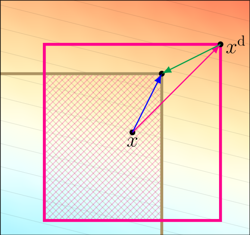
(a) Underlying space and budget constraint with $p=\infty$.

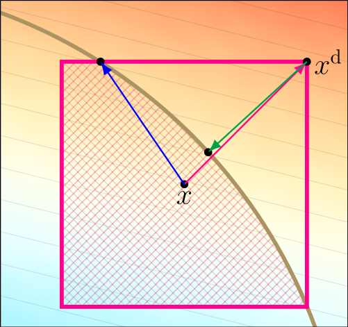
(b) Norm mismatch: underlying space with $p=\infty$ and budget constraint with $q=2$.

(c) Underlying space and budget constraint with $p=2$.

Figure 3: Visualization of one IFGSM step, employing different norm constraints and underlying norms. The beige line marks the boundary of $B_{\varepsilon}^{p}(x^{0})$, the pink line the boundary of $B_{\tau}^{q}(x)$ and the intersection $\overline{B_{\varepsilon}^{p}}(x^{0})\cap\overline{B_{\tau}^{q}}(x)$ is hatched. For the case $p=q=\infty$ minimizing a linear function on the intersection (blue arrow) is equivalent to first minimizing on $\overline{B_{\tau}^{\infty}}(x)$ (pink arrow) and then projecting back to the intersection (green arrow). This is not true for $p=2$. Therefore, we need to choose the appropriate projection in lemma 5.4.

This result shows, that when we choose $p=\infty$ for the budget constraint IFGSM again fulfills the semi-implicit minimizing movement scheme, beyond the time restriction in corollary 5.3.

Theorem 5.5.

We consider the space $(\mathcal{X},\left\|\cdot\right\|)=(\mathbb{R}^{d},\left\|\cdot\right\|_{\infty})$, $\mathcal{E}:\mathbb{R}^{d}\to\mathbb{R}$, a continuously differentiable energy, with a Lipschitz continuous gradient and choose $p=\infty$ for the budget constraint in IFGSM. Then for $T>0$, there exists a $\infty$-curve of maximal slope $u:[0,T]\to\mathbb{R}^{d}$, with respect to $\mathcal{E}$, and a subsequence of $\tau_{n}:=T/n$ such that

$$\left\|x^{\lceil t/\tau_{n_{i}}\rceil}_{\mathrm{IFGS},\tau_{n_{i}}}-u(t)\right\|\xrightarrow{i\to\infty}0\qquad\text{ for all }t\in[0,T].$$

Proof.

Since lemma 5.4 yields that IFGSM fulfills the semi-implicit minimizing movement scheme, we can proceed similarly as in the proof of corollary 5.3. We note the all the necessary assumptions are fulfilled, since the characteristic function $\chi_{\overline{B_{\varepsilon}^{\infty}}(x^{0})}$ is lower semicontinuous. ∎

5.2 Adversarial training and distributional adversaries

As before, we assume that the underlying spaces are finite dimensional, i.e., $\mathcal{X}=\mathbb{R}^{d},\mathcal{Y}=\mathbb{R}^{m}$ with norms $\left\|\cdot\right\|_{\mathcal{X}},\left\|\cdot\right\|_{\mathcal{Y}}$ and $\mathcal{P}(\mathcal{X}\times\mathcal{Y})$ denotes the space of Borel Probability measures. We consider the adversarial training task, as proposed in [53, 43],

$$\inf_{h\in\mathcal{H}}\int\sup_{\tilde{x}\in\overline{B_{\varepsilon}}(x^{0})}\ell(h(\tilde{x}),y)d\mu(x,y),$$ (5.2)

where $\mu\in\mathcal{P}(\mathcal{X}\times\mathcal{Y})$ denotes the data distribution and $l(h(x),y)\in C^{1}(\mathcal{X}\times\mathcal{Y})$. This interpretation of adversarial learning in the distributional setting has sparked a lot of interest in recent years, see e.g., [88, 94, 72, 22, 18, 73, 87, 60]. In order to rewrite this task as a distributionally robust optimization problem, we equip $\mathcal{P}(\mathcal{X}\times\mathcal{Y})$ with a suitable optimal transport distance

$$D(\mu,\tilde{\mu})\coloneqq\inf_{\gamma\in\Gamma(\mu,\tilde{\mu})}\gamma-\operatorname*{ess\,sup}\ c(x,y,\tilde{x},\tilde{y}),$$

where

$$c(x,y,\tilde{x},\tilde{y})\coloneqq\begin{cases}\|x-\tilde{x}\|_{\mathcal{X}}&\text{if }y=\tilde{y},\\ +\infty&\text{if }y\neq\tilde{y},\end{cases}$$ (5.3)

and $\Gamma(\mu,\tilde{\mu})$ denotes the set of transport plans between $\mu$ and $\tilde{\mu}$. Notably, the extended distance $c$ is not the one naturally generated by the norms of the underlying Banach spaces $\mathcal{X}$ and $\mathcal{Y}$. Nonetheless, $c$ is compatible with respect to $\|\cdot\|_{\mathcal{X}}+\|\cdot\|_{\mathcal{Y}}$ in the sense that

$$\liminf_{n\rightarrow\infty}c(x_{n},y_{n},\tilde{x}_{n},\tilde{y}_{n})\geq c(x,y,\tilde{x},\tilde{y}),$$

$$\forall(x,y),(\tilde{x},\tilde{y})\in(\mathcal{X}\times\mathcal{Y}):(x_{n},y_{n})\rightarrow(y,x),(\tilde{x}_{n},\tilde{y}_{n})\rightarrow(\tilde{x},\tilde{y})\text{ w.r.t. }\|\cdot\|_{\mathcal{X}}+\|\cdot\|_{\mathcal{Y}},$$

compare [57, Eq. (1)]. This ensures that, as we equip $\mathcal{P}(\mathcal{X}\times\mathcal{Y})$ with $D$, it is a well-defined extended distance, see [57, Section 2.6.]. The cost functional $c$ was similarly employed in [18, 13], furthermore a similar setup was considered in [88].

Remark 5.6.

Assume that $\gamma\in\Gamma(\mu,\tilde{\mu})$ is a coupling, i.e., $\gamma\in\mathcal{P}(\mathcal{Z}\times\mathcal{Z})$, where $\mathcal{Z}=\mathcal{X}\times\mathcal{Y}$, with $\gamma-\operatorname*{ess\,sup}c(x,y,\tilde{x},\tilde{y})<\infty$. Then we have that for every measurable set $A\subset\mathcal{Y}$,

$$\gamma(\mathcal{X}\times A\times\mathcal{Z})=\gamma(\mathcal{X}\times A\times\mathcal{X}\times A)=\gamma(\mathcal{Z}\times\mathcal{X}\times A),$$

which we see by contradiction: assume there exists a measurable set $A\subset\mathcal{Y}$ s.t., for $B:=\mathcal{X}\times A\times\mathcal{X}\times(\mathcal{Y}\setminus A)$ we have $\gamma(B)>0$. Then we know that $c(x,y,\tilde{x},\tilde{y})=+\infty$ for all $(x,y,\tilde{x},\tilde{y})\in B$ and since $\gamma(B)>0$ this yields that

$$\gamma-\operatorname*{ess\,sup}c(x,y,\tilde{x},\tilde{y})\geq\gamma-\operatorname*{ess\,sup}_{B}c(x,y,\tilde{x},\tilde{y})=+\infty.$$

The other identity can be proven analogously. Therefore, if $D(\mu,\tilde{\mu})<\infty$ we know that there exists a coupling $\gamma$ fulfilling the above assumption and thus for every measurable set $A\subset\mathcal{Y}$ we obtain

$$\mu(\mathcal{X}\times A)=\int_{\mathcal{X}\times A\times\mathcal{Z}}d\gamma=\int_{\mathcal{Z}\times\mathcal{X}\times A}d\gamma=\tilde{\mu}(\mathcal{X}\times A).$$

If we now consider a disintegration of $\mu$ and $\tilde{\mu}$ along the $\mathcal{X}$-axis, i.e., we obtain $d\mu=d\mu_{y}d\nu(y),d\tilde{\mu}=d\tilde{\mu}_{y}d\tilde{\nu}(y)$, with

$$\nu(A)=\mu((\pi^{y})^{-1}(A))=\mu(\mathcal{X}\times A)=\tilde{\mu}(\mathcal{X}\times A)=\tilde{\mu}((\pi^{y})^{-1}(A))=\tilde{\nu}(A)$$

for every measurable $A\subset\mathcal{Y}$, where $\pi^{y}(x,y):=y$ is the projection onto the $\mathcal{Y}$-component.

The transport distance $D$ behaves like the $\infty$-Wasserstein distance in the $\mathcal{X}$-direction (compare section section 4) and punishes movement of mass into the $\mathcal{Y}$-direction, such that no movement in $\mathcal{Y}$ can occur when $D(\mu,\tilde{\mu})$ is finite (see remark 5.6). Thus, all calculations done in section 4 apply with minor adaptation to this case. We only state corresponding lemmas and theorems, while adapted proofs can be found in appendix G. The first property we prove in this section, is that the adversarial training problem (5.2) is equivalent to the distributional robust optimization problem, DRO. Note, that now we need to consider a potential defined on the space $\mathcal{X}\times\mathcal{Y}$, namely $E(x,y)\coloneqq-\ell(h(x),y)$, where the label $y$ is now also a variable argument.

Corollary 5.7.

It holds that

$$\int\max_{\tilde{x}\in\overline{B_{\varepsilon}}(\tilde{x})}\ell(h(x),y)d\mu(x,y)=\max_{\tilde{\mu}:D(\tilde{\mu},\mu)\leq\varepsilon}\int\ell(h(x),y)d\tilde{\mu}(x,y)$$ (5.4)

where the maximizing argument is given by $\mu_{\max}=(r_{\varepsilon})_{\#}\mu$, with $r_{\varepsilon}:\mathcal{X}\times\mathcal{Y}\to\mathcal{X}$ being a $\mathcal{B}(\mathcal{X}\times\mathcal{Y})$-measurable selector from lemma G.1

Proof.

We employ the $\mathcal{B}(\mathcal{X}\times\mathcal{Y})$-measurable selector $r_{\varepsilon}$, from lemma G.1 and compute

$$\int\max_{\tilde{x}\in\overline{B_{\varepsilon}}(x)}\ell(h(\tilde{x}),y)\,d\mu(x,y) =\int\max_{(\tilde{x},\tilde{y}):c(x,y,\tilde{x},\tilde{y})\leq\varepsilon}-E(\tilde{x},\tilde{y})\,d\mu(x,y)=\int-E(r_{\varepsilon}(x,y))\,d\mu(x,y)$$

$$=-\int E(x,y)d(r_{\varepsilon})_{\#}\mu(x,y)\overset{(i)}{=}-\min_{\tilde{\mu}:D(\mu,\tilde{\mu})\leq\varepsilon}\int E(x,y)\,d\tilde{\mu}(x,y)$$

$$=\max_{\tilde{\mu}:D(\tilde{\mu},\mu)\leq\varepsilon}\int\ell(h(x),y)d\tilde{\mu}(x,y),$$

where in $(i)$ we employ G.1. ∎

For the main result in this section, we now consider the energy defined via the potential defined on $\mathcal{X}\times\mathcal{Y}$, i.e.,

$$\mathcal{G}(\mu)\coloneqq\int E(x,y)d\mu(x,y)=\int-\ell(h(x),y)d\mu(x,y),$$

where the underlying metric space is chosen as $\mathcal{D}=(\mathcal{P}(\mathcal{X}\times\mathcal{Y})_{\infty},c)$, with $\mathcal{P}(\mathcal{X}\times\mathcal{Y})_{\infty}$ denoting the subset of Borel probability measures with bounded support in $\mathcal{X}$- and $\mathcal{Y}$-direction.

Remark 5.8.

theorem 4.7 also holds for extended distances, i.e., distances which take values in $[0,+\infty]$, compare [57, Thm. 3.1]. The distance $c(\cdot,\cdot)$ introduced in equation 5.3 is such an extended distance. For this particular choice of extended distance, the measure

$$\eta\in\mathcal{P}(C(0,T;\left((\mathcal{X}\times\mathcal{Y}),\|\cdot\|_{\mathcal{X}}+\|\cdot\|_{\mathcal{Y}}\right))$$

is concentrated on $AC^{\infty}\left(0,T;\left((\mathcal{X}\times\mathcal{Y}),c\right)\right)=AC^{\infty}(0,T;(\mathcal{X},\|\cdot\|_{\mathcal{X}})\times\mathcal{Y}$. Notice that the continuous curves are continuous w.r.t. $\|\cdot\|_{\mathcal{X}}+\|\cdot\|_{\mathcal{Y}}$ while absolute continuity is w.r.t. $c(\cdot,\cdot)$(compare [57, Section 2.3.]).

The theorem below is a variant of theorem 4.19 for the adversarial setting. Namely, we show, that $\infty$-curves of maximal slope that are used to solve DRO can be characterized by employing a representing measure $\eta$ on $C(0,T;\mathcal{X}\times\mathcal{Y})$, where $\eta$-a.e. curve fulfills the differential inclusion w.r.t. the potential $E$. Here, we enforce the condition $D(\mu,\tilde{\mu})\leq\varepsilon$, by only considering the evolution until time $T=\epsilon$.

Theorem 5.9.

For $T=\varepsilon$, let $\mu\in\mathrm{AC}^{\infty}(0,T,\mathcal{D})$ with $\eta$ from theorem 4.7. Then the following statements are equivalent:

1. The curve $\mu$ is $\infty$-curve of maximal slope of the energy $\mathcal{G}$ w.r.t. to the weak upper gradient $\left|\partial\mathcal{G}\right|$.

2. For $\eta$-a.e. curve $u\in C(0,T;\mathcal{X}\times\mathcal{Y})$ it holds, that $E\circ u$ is for a.e. $t\in(0,T)$ equal to a non-increasing map $\psi_{u}$ and

   $$u^{\prime}(t)\subset(\partial\|\cdot\|_{\mathcal{X}^{*}}(-\nabla_{x}E(u(t))),0),\quad\text{for a.e. }t\in(0,T).$$

Proof.

.
Step 1 $(i)\Longrightarrow(ii)$.
Using G.2 and that equality is attained in lemma G.3, we observe that

$$(E\circ u)^{\prime}(t)=-\|\nabla_{x}E(u(t))\|_{\mathcal{X}^{*}}\quad\text{for a.e. }t\in(0,T),$$

for $\eta$-a.e. curve $u\in C(0,T,\mathcal{X}\times\mathcal{Y})$. Since $E\circ u$ is absolutely continuous we obtain by remark 1.3

$$E(u(t))-E(u(s))=\int_{s}^{t}(E\circ u)^{\prime}(r)dr=\int_{s}^{t}-\|\nabla_{x}E(u(r))\|_{\mathcal{X}^{*}}dr\leq 0$$

for all $0\leq s<t\leq T$, and thus $E\circ u$ is a non-increasing map for $\eta$-a.e. $u\in C(0,T,\mathcal{X}\times\mathcal{Y})$. We use lemma E.5 and $\||u^{\prime}|(t)\|_{L^{\infty}(\eta)}=|\mu^{\prime}|(t)\leq 1$ for a.e. $t\in(0,T)$ to infer that for $\eta$-a.e. curve $u\in C(0,T,\mathcal{X}\times\mathcal{Y})$ it holds,

$$\left|u^{\prime}\right|(t)\leq 1\quad\text{for a.e. }t\in(0,T).$$

Denoting by $(u^{\prime}(t))_{x}$ and $(u^{\prime}(t))_{y}$ the to $\mathcal{X}$ and $\mathcal{Y}$ corresponding parts of the derivative $u^{\prime}(t)$ we obtain for $\eta$-a.e. curve $u\in C(0,T,\mathcal{X}\times\mathcal{Y})$

$$\langle\nabla_{x}E(x,y),(u^{\prime}(t))_{x}\rangle =\langle\nabla E(x,y),u^{\prime}(t)\rangle$$

$$=(E\circ u)^{\prime}(t)$$

$$=-\|\nabla_{x}E(u(r))\|_{\mathcal{X}^{*}}=-\left\|\nabla_{x}E(u(r))\right\|_{\mathcal{X}^{*}}-\chi_{\overline{B_{1}}}((u^{\prime}(t))_{x})$$

for a.e. $t\in(0,T)$. Using the equivalence of A.3 (iii) and A.3 (iv) we obtain

$$u^{\prime}(t)\subset(\partial\|\cdot\|_{\mathcal{X}^{*}}(-\nabla_{x}E(x,y)),0)\quad\text{for a.e. }t\in(0,T)$$

for $\eta$-a.e. curve $u$.
Step 2 $(ii)\Longrightarrow(i)$.
For $\eta$-a.e. $u\in C(0,T;\mathcal{X}\times\mathcal{Y})$ we know by remark 2.4 that $E\circ u$ is a non-increasing map of bounded variation. In particular, it is absolutely continuous such that remark 1.3 applies. We calculate,

$$\mathcal{G}(\mu_{t}) -\mathcal{G}(\mu_{s})=\int_{C(0,T,\mathcal{X})}E(u(t))-E(u(s))d\eta(u)=\int_{C(0,T,\mathcal{X})}\int_{s}^{t}(E\circ u)^{\prime}(r)drd\eta(u)$$

$$=\int_{C(0,T,\mathcal{X})}\int_{s}^{t}\langle\nabla_{x}E(u(r)),(u^{\prime}(r))_{x}\rangle drd\eta(u)\overset{(i)}{=}\int_{C(0,T,\mathcal{X})}\int_{s}^{t}-\|\nabla_{x}E(u(r))\|_{\mathcal{X}^{*}}drd\eta(u)$$

$$=\int_{C(0,T,\mathcal{X})}\int_{s}^{t}-\|\nabla_{x}E(u(r))\|_{\mathcal{X}^{*}}d\eta(u)dr\overset{(ii)}{=}\int_{s}^{t}-|\partial\mathcal{G}|(\mu_{r})dr,$$

Where for (i) we use the equivalence of A.3 (iii) and A.3 (iv), while for (ii) we use lemma G.2. This implies $\mathcal{G}\circ\mu_{t}$ is monotone non-increasing and $(\mathcal{G}\circ\mu)^{\prime}(t)\leq-|\partial\mathcal{G}|(\mu_{t})$ for a.e. $t\in(0,T)$. Further, by theorem 4.7 we have

$$|\mu^{\prime}|(t)=\eta(u)-\operatorname*{ess\,sup}|u^{\prime}|(t)=\eta(u)-\operatorname*{ess\,sup}\|u^{\prime}(t)\|_{\mathcal{X}}\leq 1,$$

since all elements in $\partial\|\cdot\|_{\mathcal{X}^{*}}(-\nabla_{x}E(x,y))$ have norm smaller than $1$. ∎

6 Conclusion and outlook

In this work, we considered the limit case $p\to\infty$ of the well known $p$-curves of maximum slope, which yield a versatile gradient flow framework in metric spaces, [2]. In the abstract setting, we proved existence by employing the minimizing movement scheme, adapted to the case $p=\infty$. Assuming that the underlying space is Banach, we were able to characterize $\infty$-curves of maximum slope via differential inclusions. Furthermore, we also demonstrated the convergence of a semi-implicit scheme to the continuum flow. This insight constitutes the interface to the field of adversarial attacks. Namely, we showed that the well known fast gradient sign method, and its iterative variant, correspond to the semi-implicit scheme and therefore converge to the flow, when sending the step size to zero. More generally, this result holds true for a whole class of normalized gradient descent algorithms. Furthermore, we also considered Wasserstein gradient flows, where we first used the theory developed in [57] to derive an alternative characterization of absolutely continuous curves via continuity equations. As our main result in this section, we prove that being an $\infty$-curve of maximal slope is equivalent to the existence of a representing measure on the space of continuous curves, where almost every curve, fulfills a differential inclusion on the underlying Banach space. This finally allowed us to generate distributional adversaries, in an adapted $\infty$-Wasserstein distance, via curves of maximum slope. Similar to section 5 we could also consider the energy

$$G(\mu)\coloneqq\int_{\mathcal{X}\times\mathcal{Y}}E(x,y)d\mu+\chi_{B^{D}_{\epsilon}(\mu_{0})}(\mu)$$

to generate distributional adversarial attacks. We strongly suspect that corresponding $\infty$-curves of maximal slope in $\mathcal{D}$ would take the following form: Let $\mu\in AC^{\infty}(0,T;\mathcal{X})$ be a $\infty$-curve of maximal slope and $\eta$ its corresponding probability measure over the space $C(0,T;\mathcal{X}\times\mathcal{Y})$, then for $\eta$-a.e. $u\in C(0,T;\mathcal{X}\times\mathcal{Y})$

$$u^{\prime}(t)\subset(\partial\|\cdot\|_{\mathcal{X}^{*}}(-\nabla_{x}E_{u_{0}}(u(t))),0),\quad\text{for a.e. }t\in(0,T),$$

where

$$E_{u_{0}}(x,y)=E(x,y)+\chi_{B_{\epsilon}((u_{0})_{x})}(x).$$

In [92] the authors suggested to combine FGSM with stochastic elements. They proposed to use a single step

$$\sigma\sim\text{Uniform}\left(\overline{B_{\epsilon}^{\infty}}(x_{0})\right),$$

$$x_{\frac{1}{2}}=x_{0}+\sigma,$$

$$x_{1}=\mathrm{Clip}_{0,\varepsilon}\left(x_{\frac{1}{2}}+\operatorname{sign}(\nabla\ell(h(x_{\frac{1}{2}}),y))\right).$$

This is reminiscent of the classical Langevin algorithm, therefore it would be interesting if this stochasticity could be incorporated into our framework.

Appendix A Convex analysis

This section gives an overview over well-known definitions and statements in convex analysis. In the following $\mathcal{X}$ denotes a Banach space and $\mathcal{X}^{*}$ its dual.

Definition A.1 (Subdifferential).

For a convex function $f:\mathcal{X}\to(-\infty,\infty]$, we denote by

$$\partial f(x):=\{\xi\in\mathcal{X}^{*}:f(z)-f(x)\geq\langle\xi,z-x\rangle\quad\forall z\in\mathcal{X}\}\subset\mathcal{X}^{*}$$

the subdifferential of $f$ at $x\in\mathcal{X}$.

If $f(\cdot)=\|\cdot\|$ then the subdifferential is given by

$$\partial\|\cdot\|(x)=\{\xi\in\mathcal{X}^{*}|\langle\xi,x\rangle=\|x\|,\|\xi\|_{*}\leq 1\}$$ (A.1)

Definition A.2 (Fenchel conjugate).

For a function $f:\mathcal{X}\rightarrow[-\infty,+\infty]$, we denote by $f^{*}:\mathcal{X}^{*}\rightarrow[-\infty,+\infty]$,

$$f^{*}(\xi)\coloneqq\sup_{x\in\mathcal{X}}\langle\xi,x\rangle-f(x)\quad\text{for }\xi\in\mathcal{X}^{*}$$

the Fenchel conjugate of $f$.

A direct consequence of this definition is the so called Fenchel–Young inequality

$$\langle\xi,x\rangle\leq f(x)+f^{*}(\xi).$$ (A.2)

The next proposition yields the conditions under which the equality in (A.2) is obtained.

Proposition A.3 ([6, Prop. 2.33]).

Let $f:\mathcal{X}\rightarrow]-\infty,+\infty]$ be a proper convex function. Then for $x\in\mathcal{X}$, the following three properties are equivalent:

1. $\xi\in\partial f(x)$.

2. $f(x)+f^{*}(\xi)\leq\langle\xi,x\rangle$.

3. $f(x)+f^{*}(\xi)=\langle\xi,x\rangle$.

If, in addition, $f$ is lower-semicontinuous, then all of these properties are equivalent to the following one.

1. $x\in\partial f^{*}(\xi)$.

Remark A.4.

In A.3 (iv), we use the canonical embedding to obtain the subspace relation $\mathcal{X}\subset\mathcal{X}^{**}$. Following [6, Rem. 2.35], if $\mathcal{X}$ is reflexive, i.e. $\mathcal{X}^{**}=\mathcal{X}$, then it follows from Proposition A.3 that

$$x\in\partial f^{*}(\xi)\Longleftrightarrow\xi\in\partial f(x),$$

which yields

$$(\partial f)^{-1}(\xi)=\{x\in\mathcal{X}\,:\,\xi\in\partial f(x)\}=\{x\in\mathcal{X}\,:\,x\in\partial f^{*}(\xi)\}=\partial f^{*}(\xi)$$

In the non-reflexive case one can not argue as above, and we do not obtain the simple relation between $\partial f^{*}$ and $\partial f$, see, e.g., [75].

An important corollary of proposition A.3 is its application to the indicator function of the closed unit ball $f=\chi_{\overline{B_{1}}}$, where its convex conjugate for $\xi\in\mathcal{X}^{*}$ is given by

$$\chi_{\overline{B_{1}}}^{*}(\xi)=\sup_{x\in\mathcal{X}}\langle\xi,x\rangle-\chi_{\overline{B_{1}}}(x)=\sup_{x\in\overline{B_{1}}}\langle\xi,x\rangle=\|\xi\|_{*}.$$

Corollary A.5.

For a Banach space $\mathcal{X}$, and $\xi\in\mathcal{X}^{*}$ we have that

$$\partial\left\|\cdot\right\|_{*}(\xi)\cap\mathcal{X}=\operatorname*{arg\,max}_{x\in\overline{B_{1}}}\langle\xi,x\rangle.$$ (A.3)

Proof.

Since $\chi_{\overline{B_{1}}}$ is lower semicontinuous, we can use the equivalence of A.3 (iii) and A.3 (iv), to infer

$$x\in\partial\left\|\cdot\right\|_{*}(\xi)\quad\Leftrightarrow\quad\left\|\xi\right\|_{*}=\langle\xi,x\rangle-\chi_{\overline{B_{1}}}(x).$$

In the second statement, using the definition of $\left\|\xi\right\|_{*}$ as in equation A.3, therefore yields that each $x$ above realizes the supremum, which concludes the proof. ∎

Appendix B Refined version of Ascoli–Arzelà

Proposition B.1 ([2, Prop. 3.3.1]).

Let $u^{n}:[0,T]\to\mathcal{S}$ be a sequence of curves, that fulfills the following conditions:

1. There is a $\sigma$-sequentially compact set $K\subset\mathcal{S}$, such that

   $$u^{n}(t)\in K\quad\text{for every}\quad t\in[0,T]\quad\text{and every}\quad n\in\mathbb{N}.$$

2. There is a symmetric function $\omega:[0,T]\times[0,T]\to[0,+\infty)$ with $\lim_{(s,t)\to(r,r)}\omega(s,t)=0$ for all $r\in[0,T]\setminus C$, where $C$ is an at most countable set, such that

   $$\limsup_{n\to\infty}d(u^{n}(s),u^{n}(t))\leq\omega(s,t)\quad\text{for all}\quad s,t\in[0,T].$$

Then there exists a subsequence $u^{n_{k}}$ and a limit curve $u:[0,T]\to\mathcal{S}$, which is $d$-continuous in $[0,T]\setminus C$, such that

$$u^{n_{k}}(t)\overset{\sigma}{\rightharpoonup}u(t)\quad\text{for all}\quad t\in[0,T].$$

Appendix C Taylor’s formula in Banach spaces

Theorem C.1.

Suppose $E$, $F$ are real Banach spaces, $U\subset E$ an open and nonempty subset, and $f\in C^{n}(U,F)$. Given $x_{0}\in U$ choose $r>0$ such that $x_{0}+B_{r}\subset U$, where $B_{r}$ is the open ball in $E$ with center $0$ and radius $r$. Then for all $h\in B_{r}$ we have, using the abbreviation $h^{k}=(h,...,h)$, $k$ terms,

$$f(x_{0}+h)=\sum_{k=0}^{n}\frac{1}{k!}f(k)(x_{0})(h)^{k}+R_{n}(x_{0},h),$$

where the remainder $R_{n}$ is of form

$$R_{n}(x_{0},h)=\frac{1}{(n-1)!}\int_{0}^{1}(1-t)^{n-1}[f^{(n)}(x_{0}+th)-f^{(n)}(x_{0})](h)^{n}dt.$$

Proof.

A proof for this statement can be found, e.g., in [8, Thm. 30.1.3]. ∎

Appendix D Prokhorov’s theorem

Theorem D.1 (Prokhorov [7, Theorem 5.1-5.2]).

If a set $\mathcal{K}\subset\mathcal{P}(\mathcal{X})$ is tight, i.e.,

$$\forall\epsilon>0\quad\exists K_{\epsilon}\text{ compact in }\mathcal{X}\text{ such that }\mu(\mathcal{X}\setminus K_{\epsilon})\leq\epsilon\quad\forall\mu\in\mathcal{K},$$ (D.1)

then $\mathcal{K}$ is relatively compact in $\mathcal{P}(\mathcal{X})$. Conversely, if $\mathcal{X}$ is a Polish space, every relatively compact subset of $\mathcal{P}(\mathcal{X})$ is tight.

Appendix E Helpful lemmas

Lemma E.1.

Let $\phi:[0,T]\rightarrow\mathbb{R}$ be bounded from above by $C_{\max}<+\infty$ and bounded from below by $C_{\min}>-\infty$. Let further $\psi:[0,T]\rightarrow\mathbb{R}$ be non-increasing and $\phi(t)=\psi(t)$ for a.e. $t\in(0,T)$, then $\psi(t)\in[C_{\min},C_{\max}]$ for all $t\in(0,T)$.

Proof.

For every $t\in(0,T)$ we can find a sequence $\{t_{n}\}_{n\in\mathbb{N}}$, with $t_{n}\rightarrow t$, $t_{n}>t$ for all $n\in\mathbb{N}$ and $\phi(t_{n})=\psi(t_{n})$ for all $n\in\mathbb{N}$. Since $\phi(t_{n})\leq C_{\max}$ or all $n\in\mathbb{N}$ and $\psi$ is non-increasing, this implies $\psi(t)\leq C_{\max}$. The lower bound can be proven by the analogue argument. ∎

Lemma E.2.

Let $\phi:[0,T]\rightarrow\mathbb{R}$ be continuous and $\psi:[0,T]\rightarrow\mathbb{R}$ be non-increasing. If $\phi(t)=\psi(t)$ for a.e. $t\in[0,T]$, then $\phi(t)=\psi(t)$ for all $t\in(0,T)$.

Proof.

Assume there is a $t\in(0,T)$ such that $\phi(t)\not=\psi(t)$. Without loss of generality $\phi(t)>\psi(t)$. Then we can take a sequence $t_{n}$ with $t_{n}\rightarrow t$ and $\phi(t_{n})=\psi(t_{n})$ and $t_{n}>t$. The continuity of $\phi$ implies that for any $\epsilon>0$ we can choose $t_{n}$ small enough, such that $|\phi(t)-\phi(t_{n})|<\epsilon$. This contradicts the monotonicity of $\psi$, since if we choose $\epsilon<\phi(t)-\psi(t)$, we obtain a $t_{n}>t$ with $\psi(t)<\psi(t_{n})=\phi(t_{n})$. In the case $\phi(t)<\psi(t)$, we can make the same argument with sequences $t_{n}<t$. ∎

Lemma E.3.

Let $\mu$ be a Borel probability measure on $\mathcal{X}$ and $v:\mathcal{X}\rightarrow\mathcal{X}$, $\tilde{v}:\mathcal{X}\rightarrow\mathcal{X}$ be two $\mu$-measurable functions with

$$\int\langle D\varphi(x),v(x)\rangle d\mu(x)=\int\langle D\varphi(x),\tilde{v}(x)\rangle d\mu(x)\quad\forall\varphi\in C^{1}_{b}(\mathcal{X})$$

then

$$\int\langle\xi,v(x)\rangle d\mu(x)=\int\langle\xi,\tilde{v}(x)\rangle d\mu(x)\quad\forall\xi\in\mathcal{X}^{*}.$$ (E.1)

Proof.

Let $g_{n}:\mathbb{R}\rightarrow\mathbb{R}$ be the function with $g(0)=0$ and

$$g^{\prime}(x)=\begin{cases}0&\text{for }|x|>n+1,\\ 1&\text{for }|x|<n,\\ n+1-x&\text{for }x\in[n,n+1],\\ n+1+x&\text{for }x\in[-(n+1),-n].\end{cases}$$

Then for each $\xi\in\mathcal{X}^{*}$ we get $G_{n}:x\mapsto g_{n}(\langle\xi,x\rangle)\in C^{1}_{b}(\mathcal{X})$ with $DG_{n}(x)=g_{n}^{\prime}(\langle\xi,x\rangle)\ \xi$ and

$$\int g_{n}^{\prime}(\langle\xi,x\rangle)\langle\xi,v(x)\rangle d\mu =\int\langle DG_{n}(x),v(x)\rangle d\mu=\int\langle DG_{n}(x),\tilde{v}(x)\rangle d\mu$$

$$=\int g^{\prime}_{n}(\langle\xi,x\rangle)\langle\xi,\tilde{v}(x)\rangle d\mu$$

Since for $n\rightarrow\infty$ we have $g^{\prime}(\langle\xi,x\rangle)\rightarrow 1$ pointwise we can apply the Lebesgue dominated convergence theorem (with the functions $|\langle\xi,v(x)\rangle|$ and $|\langle\xi,\tilde{v}(x)\rangle|$ as bound) to obtain (E.1). ∎

The following lemma, shows that the disintegration property can be transferred to an inequality for essential suprema. For more details on disintegration, we refer to [2, Ch. 5.3] and [31, Ch. III-70]. The proof strategy is taken from [77, Lem. 2] and amounts to controlling the null sets of the measures involved.

Lemma E.4.

Given $\mathcal{X},\mathcal{Z}$ Radon separable metric spaces, a measure $\mu\in\mathcal{P}(\mathcal{X})$, a Borel map $\pi:\mathcal{X}\to\mathcal{Z}$ and a disintegration $d\mu=d\mu_{z}d\nu$, with $\nu=\pi_{\#}\mu$ and $\{\mu_{z}\}_{z\in\mathcal{Z}}\subset\mathcal{P}(\mathcal{X})$ being a family of probability measures, then we have that

$$\mu(x)-\operatorname*{ess\,sup}f(x)\geq\nu(z)-\operatorname*{ess\,sup}\,\mu_{z}(x)-\operatorname*{ess\,sup}f(x)$$

for every Borel map $f:\mathcal{X}\to[0,\infty]$.

Proof.

Using the disintegration property, for every Borel set $A$ we obtain

$$\mu(A)=0\quad\Leftrightarrow\quad\mu_{z}(A)\text{ for }\nu-\text{a.e. }z\in\mathcal{Z}.$$

Now assume that $\mu(A)=0$, then we know that there exists a Borel set $B\subset\mathcal{Z}$ with $\nu(B)=0$ and $\mu_{z}(A)=0$ for all $z\in\mathcal{Z}\setminus B$. Therefore,

$$\sup_{x\in\mathcal{X}\setminus A}f(x) \geq\inf_{\tilde{A}:\mu_{z}(\tilde{A})=0}\sup_{x\in\mathcal{X}\setminus\tilde{A}}f(x)=\mu_{z}(x)-\operatorname*{ess\,sup}f(x)\qquad\text{ for all }z\in\mathcal{Z}\setminus B$$

$$\Rightarrow\sup_{x\in\mathcal{X}\setminus A}f(x) \geq\sup_{z\in\mathcal{Z}\setminus B}\,\mu_{z}(x)-\operatorname*{ess\,sup}f(x)$$

$$\geq\inf_{\tilde{B}:\nu(\tilde{B})=0}\sup_{z\in\mathcal{Z}\setminus\tilde{B}}\mu_{z}(x)-\operatorname*{ess\,sup}f(x)$$

$$=\nu(z)-\operatorname*{ess\,sup}\,\mu_{z}(x)-\operatorname*{ess\,sup}f(x)$$

and since this holds for every $\mu$-null set $A$, we can take the infimum to obtain

$$\mu(x)-\operatorname*{ess\,sup}f(x)=\inf_{A:\mu(A)=0}\sup_{x\in\mathcal{X}\setminus A}f(x)\geq\nu(z)-\operatorname*{ess\,sup}\,\mu_{z}(x)-\operatorname*{ess\,sup}f(x).$$

∎

Lemma E.5.

Let $\eta\in\mathcal{P}(C(0,T;\mathcal{X}))$, then we have that

$$\eta(u)-\operatorname*{ess\,sup}\left|u^{\prime}\right|(t)\leq 1\quad \text{for a.e. }t\in(0,T)\Longleftrightarrow\operatorname*{ess\,sup}_{t\in(0,T)}\,\left|u^{\prime}\right|(t)\leq 1\quad \text{for }\eta\text{ a.e. }u\in C(0,T;\mathcal{X}).$$

Proof.

Choosing $\psi=\chi_{[0,1]}$, and observing that $\psi(|u^{\prime}|(t))$ is $\bar{\eta}$-measurable (see [57, Eq. 55]) implies

$$\eta(u)-\operatorname*{ess\,sup}\left|u^{\prime}\right|(t)\leq 1\quad \text{for a.e. }t\in(0,T)$$

$$\Longleftrightarrow\int_{C(0,T,\mathcal{X})}\psi(\left|u^{\prime}\right|(t))d\eta(u)=0\quad\text{for a.e. }t\in(0,T)$$

$$\Longleftrightarrow\int_{0}^{T}\int_{C(0,T,\mathcal{X})}\psi(\left|u^{\prime}\right|(t))d\eta(u)dt=0 \Longleftrightarrow\int_{C(0,T,\mathcal{X})}\int_{0}^{T}\psi(\left|u^{\prime}\right|(t))d\eta(u)dt=0$$

$$\Longleftrightarrow\int_{C(0,T,\mathcal{X})}\int_{0}^{T}\psi(\left|u^{\prime}\right|(t))dtd\eta(u)=0 \Longleftrightarrow\int_{0}^{T}\psi(\left|u^{\prime}\right|(t))dt=0\quad\text{for }\eta\text{ a.e. }u\in C(0,T;\mathcal{X})$$

$$\Longleftrightarrow\operatorname*{ess\,sup}_{t\in(0,T)}\,\left|u^{\prime}\right|(t)\leq 1\quad \text{for }\eta\text{ a.e. }u\in C(0,T;\mathcal{X}),$$

where we use Fubini–Tonelli theorem to change the order of integration. ∎

Appendix F Multivalued correspondences

For multivalued correspondences, generalizations of continuity and measurability can be defined. We use the definitions from [23]. In the following, we write $\varphi:\mathcal{X}\rightrightarrows\mathcal{Z}$ to denote a mapping $\varphi:\mathcal{X}\to 2^{\mathcal{Z}}$.

Definition F.1 (Weak measurability).

Let $(S,\Sigma)$ be a measurable space and $\mathcal{X}$ be a topological space. We say that a correspondence $\varphi:S\rightrightarrows\mathcal{X}$ is weakly measurable, if

$$\varphi^{l}(G)\in\Sigma\text{ for all open sets }G\text{ of }\mathcal{X},$$

where

$$\varphi^{l}(G)\coloneqq\{s\in S|\varphi(s)\cap G\neq\emptyset\}$$

is the so-called lower inverse.

Definition F.2 (Measurability).

Let $(S,\Sigma)$ be a measurable space and $\mathcal{X}$ a topological space. We say that a correspondence $\varphi:S\rightrightarrows\mathcal{X}$ is measurable, if

$$\varphi^{l}(F)\in\Sigma\text{ for all closed sets }F\text{ of }\mathcal{X}.$$

The next theorem is known as the measurable maximum theorem, where we refer to [23, Thm. 18.19] for the proof of this statement.

Theorem F.3 (Measurable Maximum Theorem).

Let $\mathcal{X}$ be a separable metrizable space and $(S,\Sigma)$ a measurable space. Let $\varphi:S\rightrightarrows\mathcal{X}$ be a weakly measurable correspondence with nonempty compact values, and suppose $f:S\times\mathcal{X}\rightarrow\mathbb{R}$ is a Carathéodory function. Define the value function $m:S\rightarrow\mathbb{R}$ by

$$m(s)=\max_{x\in\varphi(s)}f(s,x),$$

and the correspondence $\mu:S\rightrightarrows\mathcal{X}$ of maximizers by

$$\mu(s)=\{x\in\varphi(s):f(s,x)=m(s)\}.$$

Then

• The value function $m$ is measurable.

• The “argmax” correspondence $\mu$ has nonempty and compact values.

• The “argmax” correspondence $\mu$ is measurable and admits a measurable selector.

Appendix G Calculations for distributional adversaries

For completeness, we state all lemmas used in section 5.2 here. Those lemmas correspond to a lemma proven in section section 4.3 and are only adapted to the setting of the transport distance $D$.

Lemma G.1.

Let $\mathcal{X}\times\mathcal{Y}=\mathbb{R}^{d}\times\mathbb{R}^{m}$, then the correspondence

$$\bm{r}_{\varepsilon}(x,y)=\operatorname*{arg\,min}_{(\tilde{x},\tilde{y}):c(x,y,\tilde{x},\tilde{y})\leq\varepsilon}E(\tilde{x},\tilde{y})=\left(\operatorname*{arg\,min}_{\tilde{x}\in\overline{B_{\varepsilon}}(x)}E(\tilde{x},y),y\right)$$

is measurable and admits a $\mathcal{B}(\mathcal{X}\times\mathcal{Y})$-measurable selector. Further, for each measurable selector $r_{\varepsilon}:\mathcal{X}\times\mathcal{Y}\to\mathcal{X}$ we have the following,

$$(r_{\varepsilon})_{\#}(\mu)\in\operatorname*{arg\,min}_{D(\mu,\tilde{\mu})\leq\varepsilon}\int E(x,y)d\mu(x,y).$$ (G.1)

Proof.

We consider the correspondence $\varphi:\mathcal{X}\times\mathcal{Y}\rightrightarrows\mathcal{X}\times\mathcal{Y}$ given by

$$(x,y)\mapsto\left(\overline{B_{\varepsilon}}(x),y\right)$$

where on the input space we use the topology induced by $\|\cdot\|_{\mathcal{X}}+\|\cdot\|_{\mathcal{Y}}$ and the output space is interpreted as the standard Euclidean space. Then we have that for every open set $G\in\mathcal{X}$ that

$$\varphi^{l}(G)=\{(x,y)\in\mathcal{X}\times\mathcal{Y}\,:\,\left(\overline{B_{\varepsilon}}(x),y\right)\cap G\neq\emptyset\}\subset\mathcal{B}(\mathcal{X}\times\mathcal{Y}),$$

is open, which implies weak measurability, according to definition F.1. Furthermore, we define the map $f((x,y),(\tilde{x},\tilde{y})):=-E(\tilde{x},\tilde{y})$ which is a Carathéodory function, since $E$ is continuous, with

$$\max_{(\tilde{x},\tilde{y})\in\varphi(x,y)}f((x,y),(\tilde{x},\tilde{y}))=\min_{(\tilde{x},\tilde{y}):c(x,y,\tilde{x},\tilde{y})\leq\epsilon}-E(\tilde{x},\tilde{y})$$

Then theorem F.3 ensures the existence of a measurable selector. To prove equation G.1 we observe that if $D(\mu,\tilde{\mu})\leq\varepsilon$, then for an optimal transport plan $\gamma\in\Gamma_{0}(\mu,\tilde{\mu})$, we know that $y=\tilde{y}$ and $\|x-\tilde{x}\|\leq\varepsilon$, $\gamma$-a.e. Thus, using the disintegration $d\gamma(x,y,\tilde{x},\tilde{y})=d\psi_{x,y}(\tilde{x},\tilde{y})d\mu(x,y)$, for every $\tilde{\mu}$ with $D(\tilde{\mu},\mu)\leq\varepsilon$, we calculate

$$\int E(\tilde{x},\tilde{y})d\tilde{\mu}(\tilde{x},\tilde{y})=\int E(\tilde{x},\tilde{y})d\gamma(x,y,\tilde{x},\tilde{y})=\int\int E(\tilde{x},\tilde{y})d\psi_{x,y}(\tilde{x},\tilde{y})d\mu(x,y)$$

$$=\int\int E(\tilde{x},y)d\psi_{x,y}(\tilde{x},\tilde{y})d\mu(x,y)\geq\int\int E(r_{\varepsilon}(x,y))d\psi_{x,y}(\tilde{x},\tilde{y})d\mu(x,y)=\int E(r_{\varepsilon}(x,y))d\mu(x,y),$$

and equation G.1 follows. ∎

Lemma G.2.

Let $\mathcal{X}\times\mathcal{Y}=\mathbb{R}^{d}\times\mathbb{R}^{m}$, $E:\mathcal{X}\times\mathcal{Y}\rightarrow\mathbb{R}$ be in $C^{1}(\mathcal{X}\times\mathcal{Y})$ and $\mu\in\mathcal{P}_{\infty}(\mathcal{X}\times\mathcal{Y})$ , then the metric slope with respect to $D$ is given by

$$|\partial\mathcal{G}|(\mu)=\int\|\nabla_{x}E(x,y)\|_{\mathcal{X}^{*}}d\mu.$$

Proof.

By lemma G.1 we obtain

$$|\partial\mathcal{G}|(\mu)=\limsup_{\tau\rightarrow 0}\frac{\mathcal{G}(\mu)-\mathcal{G}_{\tau}(\mu)}{\tau}=\limsup_{\tau\rightarrow 0}\int\frac{E(x,y)-E(r_{\tau}(x,y))}{\tau}d\mu$$

$$=\int\lim_{\tau\rightarrow 0}\frac{E(x,y)-E(r_{\tau}(x,y))}{\tau}d\mu=\int\|\nabla_{x}E(x,y)\|_{\mathcal{X}^{*}}d\mu,$$

where dominated convergence together with lemma 3.6 and 3.1 (iii) was used to draw the limit into the integral. ∎

Lemma G.3.

Let $\mu\in\mathrm{AC}^{\infty}(0,T;\mathcal{D})$ be a curve of maximal slope of the energy $\mathcal{G}:\mathcal{P}(\mathcal{X}\times\mathcal{Y})\rightarrow\mathbb{R}$ with respect to the upper gradient $|\partial\mathcal{G}|$. Then $\mu$ satisfies the energy dissipation equality, i.e.,

$$\mathcal{G}(\mu_{t})-\mathcal{G}(\mu_{s})=-\int_{s}^{t}|\partial\mathcal{G}|(\mu_{r})dr\quad 0\leq s\leq t\leq T.$$

Proof.

By remark 2.4 we know that the non-increasing map $\psi$ from definition 1.10 is of bounded variation and in particular $-\psi^{\prime}(t)\in L^{1}(0,T)$. Therefore, we can estimate

$$|\mathcal{G}(\mu_{t})-\mathcal{G}(\mu_{s})| \leq\int_{C(0,T;\mathcal{X})}|E(u(t))-E(u(s))|d\eta(u)$$

$$=\int_{C(0,T;\mathcal{X})}\left|\int_{s}^{t}\langle\nabla E(u(r)),u^{\prime}(r)\rangle dr\right|d\eta(u)$$

$$\overset{(i)}{\leq}\int_{C(0,T;\mathcal{X})}\int_{s}^{t}\|\nabla_{x}E(x,y)\|_{\mathcal{X}^{*}}drd\eta(u)$$

$$=\int_{s}^{t}\int_{C(0,T;\mathcal{X})}\|\nabla_{x}E(x,y)\|_{\mathcal{X}^{*}}d\eta(u)dr=\int_{s}^{t}|\partial\mathcal{G}|(u(r))dr,$$

where for (i) we observe that $u^{\prime}(t)$ is $0$ in its corresponding $y$-component and the last equality follows from lemma G.2. This implies that $\mathcal{G}\circ u$ is absolutely continuous and its derivative is defined for a.e. $t\in(0,T)$. To obtain the dissipation inequality, we use the estimates

$$\mathcal{G}(\mu_{t})-\mathcal{G}(\mu_{s})=\int_{s}^{t}(\mathcal{G}\circ u)^{\prime}(r)dr=\int_{s}^{t}\psi^{\prime}(r)dr\leq\int_{s}^{t}-|\partial\mathcal{G}|(\mu_{r})dr\quad\text{for }0\leq s\leq t\leq T.$$

and

$$\begin{aligned} \mathcal{G}(\mu_{t})-\mathcal{G}(\mu_{s})=&\int_{C(0,T;\mathcal{X})}\int_{s}^{t}(E\circ u)^{\prime}(r)dr\,d\eta(u)\\ \geq&\int_{C(0,T;\mathcal{X})}\int_{s}^{t}-|\langle\nabla E(x,y),u^{\prime}(r)\rangle|dr\,d\eta(u)\\ \geq&\int_{s}^{t}\int_{C(0,T;\mathcal{X})}-\|\nabla_{x}E(x,y)\|_{{\mathcal{X}}^{*}}(u(r))d\eta(u)\,dr=\int_{s}^{t}-|\partial\mathcal{G}|(\mu_{r})dr.\end{aligned}$$ (G.2)

∎

Appendix H Details on numerical examples

Here, we give some details on the experiment that produces figure 1, the source code is provided at github.com/TimRoith/AdversarialFlows.

H.1 Training the neural network

We sample $K=1000$ labeled data points $((x_{1},y_{1}),\ldots,(x_{K},y_{K}))$, with $x_{k}\in\mathbb{R}^{2},y_{k}\in\{0,1\}$, from the two moons data set using the sci-kit package [69], see figure 4(a).

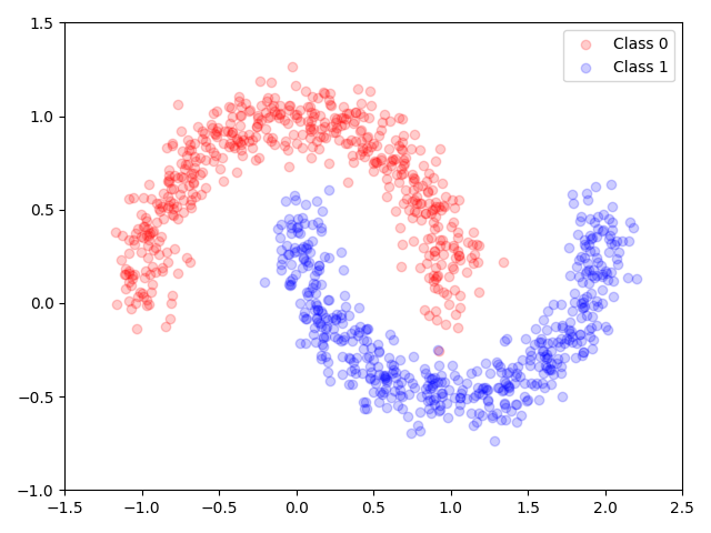
(a) The dataset used to train a binary classifier.

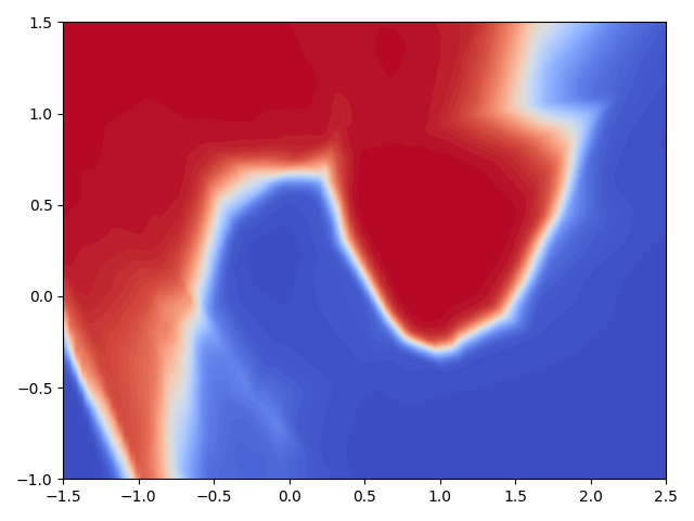
(b) The trained classifier, with ReLU activation, evaluated on the domain $[-1.5,2.5]\times[-1.,1.5]$.

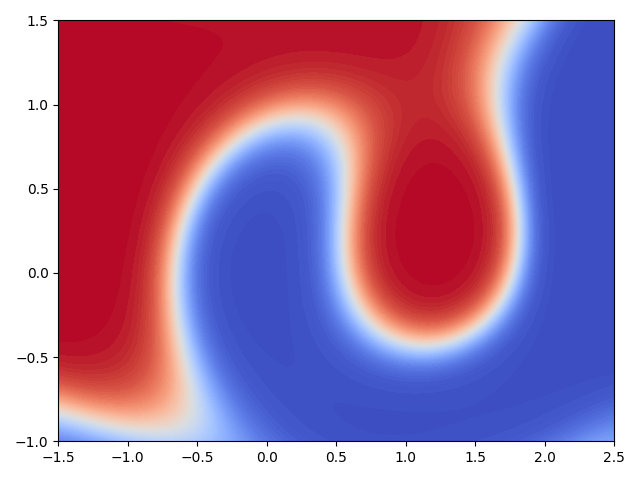
(c) The trained classifier, with GeLU activation, evaluated on the domain $[-1.5,2.5]\times[-1.,1.5]$.

Using PyTorch [67], we then train a neural network using the architecture displayed in figure 5 as proposed in [47], to obtain a mapping $h_{\theta}:\mathbb{R}^{2}\to[0,1]$, parametrized by $\theta$. Here “Linear $d^{l}\to d^{l+1}$” in the $l$th layer, denotes an affine linear mapping [78] given by

$$z\mapsto Wz+b,\qquad\text{with learnable parameters}\quad W\in\mathbb{R}^{d^{l+1}\times d^{l}},b\in\mathbb{R}^{d^{l+1}}$$

the activation functions “ReLU” [40], “GeLU” [46] and “Sigmoid” are defined entry-wise for $i=1,\ldots,n$, as

$$\text{ReLU}(z_{i}):=\max\{0,z_{i}\},\qquad\text{GeLU}(z_{i}):=z_{i}\cdot\Phi(z_{i}),\qquad\text{Sigmoid}(z_{i}):=\frac{1}{1+\exp(-z_{i})},$$

where $\Phi$ denotes the cumulative distribution function of the standard normal distribution. Here, we included both ReLU and GeLU (as a smooth approximation) to have an activation function, typically used in practice and a differentiable approximation fitting into the framework of section 3.3. During training, we process batches of inputs $\mathbf{z}=(z^{1},\ldots,z^{B})$, with $z_{i}\in\mathbb{R}^{d^{l}}$, where “Batch Norm ($B$)”, as proposed in [49], uses the entry-wise mean $\mu(\mathbf{z})_{i}:=\frac{1}{B}\sum_{b=1}^{B}z_{i}^{b}$ and variance $\sigma(\mathbf{z})_{i}:=\frac{1}{B}\sum_{b=1}^{B}(z_{i}^{b}-\mu(\mathbf{z}))^{2}$ and is defined as

$$z_{i}^{b}\mapsto\frac{z_{i}^{b}-\mu(\mathbf{z})_{i}}{\sqrt{\sigma(\mathbf{z})_{i}^{2}+\epsilon}}\cdot\gamma_{i}+\beta_{k},\qquad\text{with learnable parameters}\quad\gamma,\beta\in\mathbb{R}^{d^{l}},$$

where $\epsilon=10^{-5}$ is a small constant, added for numerical stability. During inference, the mean and variance are replaced by an estimate over the whole dataset, such that the output does not depend on the batch it is given. In total, $\theta$ denotes the collection of weights $W$, biases $b$ and batch norm parameters $\gamma,\beta$ of all layers. For training, we consider the loss function

$$\mathcal{L}(\theta)=\frac{1}{2K}\sum_{k=1}^{K}\left|h_{\theta}(x_{k})-y_{k}\right|^{2},$$ (H.1)

where we employ the Adam optimizer [51], with standard learning rates, to approximate a minimizer. In each step, we employ a batched version of the function in equation H.1, i.e., instead of using all data points at once, in each so-called epoch, we randomly sample disjoint subsets of $\{1,\ldots,K\}$, of size $B=100$ and only sum over these points. We run this training process for a total of $100$ epochs, to obtain a set of parameters $\theta^{*}$, with a train loss of approximately $\mathcal{L}(\theta^{*})\approx 0.002$ for ReLU and $\mathcal{L}(\theta^{*})\approx 0.009$ for GeLU. The trained mappings $h_{\theta}$ are visualized in figures 4(b) and 4(c).

Figure 5: The network architecture used in the examples.

H.2 Computing IGFSM and the minimizing movement scheme

We now detail the iteration as displayed in figure 1, first for ReLU. Here, we choose the initial value $x^{0}=(0.1,0.55)$, as it is close to the decision boundary, with $h_{\theta^{*}}(x^{0})\approx 0.97$, an adversarial budget of $\varepsilon=0.2$ and the energy

$$\mathcal{E}(x):=\left|h_{\theta^{*}}(x)-1\right|^{2}+\chi_{B_{\varepsilon}^{\infty}(x^{0})}.$$

IFGSM is an explicit iteration and can therefore be implemented directly, where the gradient is computed with the automatic differentiation tools of PyTorch. For the minimizing movement scheme MinMove, we need to solve the problem

$$x_{\tau}^{k+1}\in\operatorname*{arg\,min}_{x\in\overline{B_{\tau}^{\infty}}(x_{\tau}^{k})\cap\overline{B_{\varepsilon}^{\infty}}(x^{0})}\mathcal{E}(x),$$

in each step. In order to avoid local minima, we do not employ a gradient based method here, but rather a particle based method, which allows exploring the full rectangle $\overline{B_{\tau}^{\infty}}(x_{\tau}^{k})$. We use consensus based optimization (CBO) as proposed in [70], using the CBXPy package [4]. Concerning the hyperparameters, we choose $N=30$ particles, a noise scaling of $\sigma=2$, with standard isotropic noise, a time discretization parameter $dt=0.01$, $\alpha=10^{8}$ and perform $30$ update steps in each inner iteration. In order to ensure the budget constraint and the local restriction given by the step size $\tau$, we project the ensemble of the CBO iteration to the set

$$\overline{B^{\infty}_{\varepsilon}}(x^{0})\cap\overline{B^{\infty}_{\tau}}(x^{k}_{\tau})$$

using the $\ell^{\infty}$ projection, i.e., a clipping operation. We repeat the experiment for GeLU with a different initial value $x^{0}=(0.45,0.3),h_{\theta^{*}}(x^{0})\approx 0.74$ and budget $\varepsilon=0.25$, which is displayed in figure 6.

g IFGSM

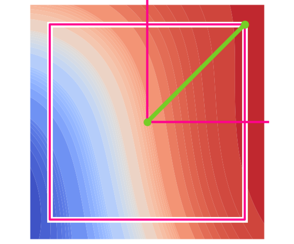
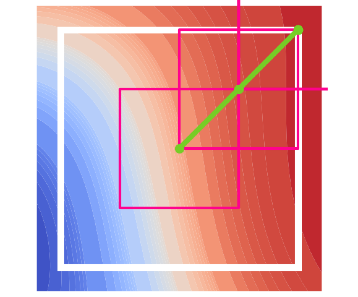
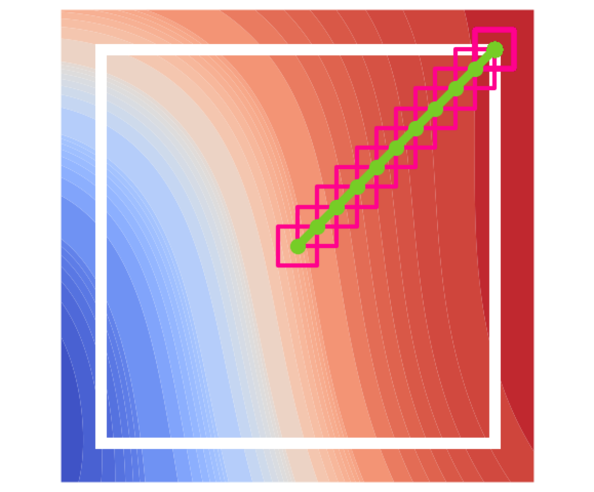
— Minimizing Movement

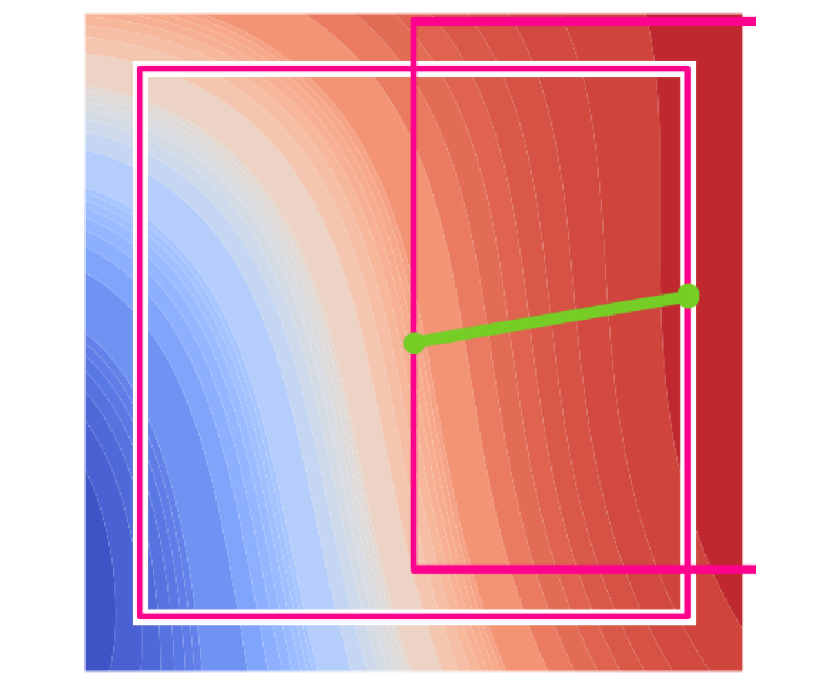
(a) $\tau=0.25$

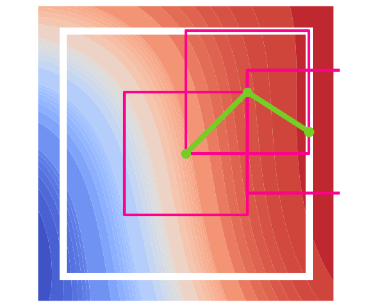
(b) $\tau=0.125$

(c) $\tau=0.025$

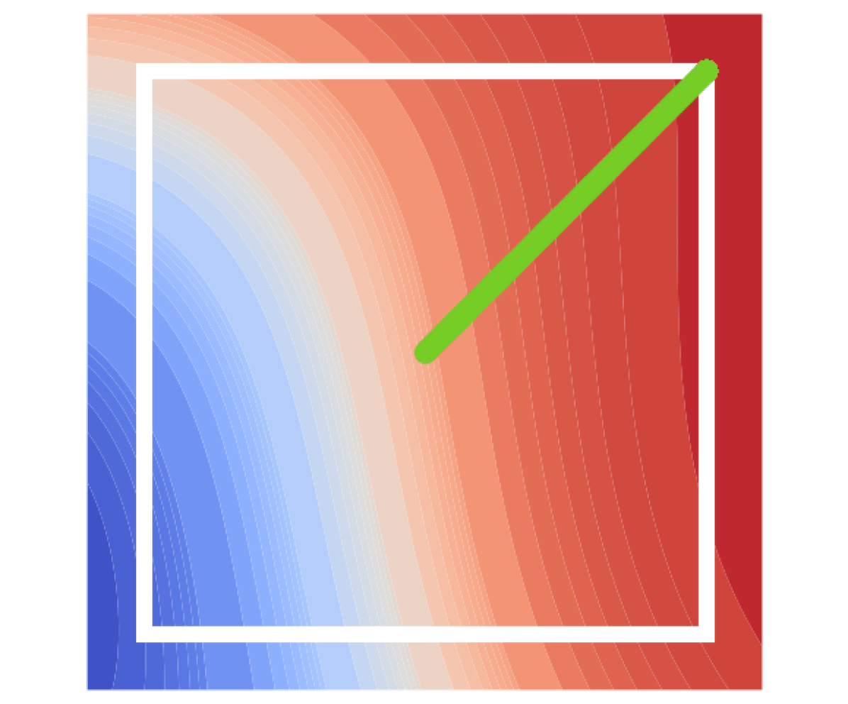
(d) $\tau=0.001$

Figure 6: The same experiment as in figure 1, but using a net employing the GeLU activation function.

H.3 Convergence of the standard and semi-implicit scheme

In this section, we consider the error between the standard and the semi-implicit minimizing movement, which serves as a very basic validation of the numerical schemes. Our theoretical framework shows that both iterations converge to a $\infty$-curve of maximum slope, which however is not available numerically. Instead, for $n\in\mathbb{N}$ and $k\leq n$, we can consider

$$\left\|x^{k}_{\mathrm{si},\tau_{n}}-x^{k}_{\tau_{n}}\right\|_{\infty}\leq\left\|x^{k}_{\mathrm{si},\tau_{n}}-u(k\cdot\tau_{n})\right\|_{\infty}+\left\|x^{k}_{\tau_{n}}-u(k\cdot\tau_{n})\right\|_{\infty},$$

where $x^{k}_{\tau_{n}}$ fulfills the standard minimizing movement scheme and $x^{k}_{\mathrm{si},\tau_{n}}=x^{k}_{\mathrm{IFGS},\tau}$ is given by IFGSM, i.e., fulfills the semi-implicit scheme. Although, our theory does not provide concrete estimates or rates of the error between IFGSM and the minimizing movement scheme, we perform a small numerical experiment using the setup from above. For each choice of $\tau$ we sample $S=50$ different initial values $x^{0,s}$ and compute the iterates $x^{k,s}_{\mathrm{IFGS}}$ and $x^{k,s}_{\tau}$ for $k\in\{1,\ldots,\lfloor 1/\tau\rfloor\}$ and compute the averaged maximal distance

$$e_{\tau}:=\frac{1}{S}\sum_{s=1}^{S}\max_{k}\left\|x^{k,s}_{\mathrm{IFGS}}-x^{k,s}_{\tau}\right\|_{\infty}.$$ (H.2)

The errors are plotted in figure 7(a). In both cases the errors converge to zero, however we observe that the order of convergence is higher for the GeLU function. We note that our theoretical results only provide a convergence statement for the differentiable case, therefore these results are in line with the analysis. In particular lemma 3.12 requires a Lipschitz differentiable gradient. However, we hypothesize that the slower convergence in the ReLU case, actually comes from the non-implicit error as visualized in figure 7(b). There we mimic a situation enforced by the ReLU activation function. For $\tau>0.1$, the minimizing movement scheme always “jumps” across the non-differentiable line $x_{1}=0.1$, to the corner where the minimum on $\overline{B_{\tau}^{\infty}}(x^{0})$ is attained, which leads the following iterates to follow the gradient into the direction $(1,1)$. However, in this case the actual flow is given as $u(t):=(t,0)$, which, in this case, is more accurately prescribed by FGSM. In this regard, a more exhaustive study, both empirically and theoretically is required, which is left for future work.

(a) Difference between IFGSM and the minimizing movement scheme, as defined in equation H.2, for different values of $\tau$, using ReLU and GeLU activation functions in the network architecture.

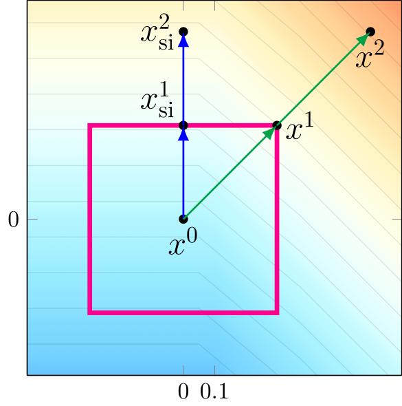
(b) Minimizing movement scheme (blue arrows) and semi-implicit version (green arrows) for the function $\mathcal{E}(x):=-x_{2}-\max\{x_{1},0.1\}$ starting from $x^{0}=(0,0)$.

Figure 7:

References

- [1] Luigi Ambrosio “Metric space valued functions of bounded variation” In Annali della Scuola Normale Superiore di Pisa-Classe di Scienze 17.3, 1990, pp. 439–478
- [2] Luigi Ambrosio, Nicola Gigli and Giuseppe Savaré “Gradient flows: in metric spaces and in the space of probability measures” Springer Science & Business Media, 2005
- [3] Scott N Armstrong and Charles K Smart “An easy proof of Jensen’s theorem on the uniqueness of infinity harmonic functions” In Calculus of Variations and Partial Differential Equations 37 Springer, 2010, pp. 381–384
- [4] Rafael Bailo, Alethea Barbaro, Susana N. Gomes, Konstantin Riedl, Tim Roith, Claudia Totzeck and Urbain Vaes “CBX: Python and Julia packages for consensus-based interacting particle methods”, 2024 arXiv:2403.14470 [math.OC]
- [5] Lukas Balles, Fabian Pedregosa and Nicolas Le Roux “The Geometry of Sign Gradient Descent”, 2020 arXiv:2002.08056
- [6] Viorel Barbu and Teodor Precupanu “Convexity and optimization in Banach spaces” Springer Science & Business Media, 2012
- [7] Patrick Billingsley “Convergence of probability measures” John Wiley & Sons, 2013
- [8] Philippe Blanchard and Erwin Brüning “Mathematical methods in Physics: Distributions, Hilbert space operators, variational methods, and applications in quantum physics” Birkhäuser, 2015
- [9] Ludwig Boltzmann “Studien über das Gleichgewicht der lebenden Kraft” In Wissenschafiliche Abhandlungen 1 Barth, 1868, pp. 49–96
- [10] Lorenzo Brasco and Filippo Santambrogio “An equivalent path functional formulation of branched transportation problems” In Discrete and Continuous Dynamical Systems 29, 2011, pp. 845–871 DOI: 10.3934/dcds.2011.29.845
- [11] Wieland Brendel, Jonas Rauber and Matthias Bethge “Decision-based adversarial attacks: Reliable attacks against black-box machine learning models” In arXiv preprint arXiv:1712.04248, 2017
- [12] Wieland Brendel, Jonas Rauber, Matthias Kümmerer, Ivan Ustyuzhaninov and Matthias Bethge “Accurate, reliable and fast robustness evaluation” In Advances in neural information processing systems 32, 2019
- [13] Tuan Anh Bui, Trung Le, Quan Tran, He Zhao and Dinh Phung “A unified wasserstein distributional robustness framework for adversarial training” In arXiv preprint arXiv:2202.13437, 2022
- [14] Leon Bungert and Martin Burger “Asymptotic profiles of nonlinear homogeneous evolution equations of gradient flow type” In Journal of Evolution Equations 20.3 Springer, 2020, pp. 1061–1092
- [15] Leon Bungert, Martin Burger, Antonin Chambolle and Matteo Novaga “Nonlinear spectral decompositions by gradient flows of one-homogeneous functionals” In Analysis & PDE 14.3 Mathematical Sciences Publishers, 2021, pp. 823–860
- [16] Leon Bungert, Jeff Calder and Tim Roith “Uniform convergence rates for Lipschitz learning on graphs” In IMA Journal of Numerical Analysis 43.4 Oxford University Press, 2023, pp. 2445–2495
- [17] Leon Bungert, Jeff Calder and Tim Roith “Ratio convergence rates for Euclidean first-passage percolation: Applications to the graph infinity Laplacian” In The Annals of Applied Probability, 2024 eprint: 2210.09023
- [18] Leon Bungert, Nicolás García Trillos and Ryan Murray “The geometry of adversarial training in binary classification” In Information and Inference: A Journal of the IMA 12.2 Oxford University Press, 2023, pp. 921–968
- [19] Leon Bungert, Tim Laux and Kerrek Stinson “A mean curvature flow arising in adversarial training”, 2024 arXiv:2404.14402
- [20] Leon Bungert, René Raab, Tim Roith, Leo Schwinn and Daniel Tenbrinck “CLIP: Cheap Lipschitz training of neural networks” In Scale Space and Variational Methods in Computer Vision: 8th International Conference, SSVM 2021, Proceedings, 2021, pp. 307–319 Springer DOI: 10.1007/978-3-030-75549-2_25
- [21] Leon Bungert and Kerrek Stinson “Gamma-convergence of a nonlocal perimeter arising in adversarial machine learning” In Calculus of Variations and Partial Differential Equations 63.5 Springer, 2024, pp. 114
- [22] Leon Bungert, Nicolás García Trillos, Matt Jacobs, Daniel McKenzie, Đorđe Nikolić and Qingsong Wang “It begins with a boundary: A geometric view on probabilistically robust learning”, 2023 arXiv:2305.18779
- [23] Kim C. Charalambos D. “Infinite dimensional analysis” Springer, 2006
- [24] Fei Chen and Wei Ren “Sign projected gradient flow: A continuous-time approach to convex optimization with linear equality constraints” In Automatica 120, 2020, pp. 109156 DOI: https://doi.org/10.1016/j.automatica.2020.109156
- [25] Evgenii Chzhen and Sholom Schechtman “SignSVRG: fixing SignSGD via variance reduction”, 2023 arXiv:2305.13187 [math.OC]
- [26] Jorge Cortés “Finite-time convergent gradient flows with applications to network consensus” In Automatica 42.11 Elsevier, 2006, pp. 1993–2000
- [27] George Cybenko, Dianne P O’Leary and Jorma Rissanen “The mathematics of information coding, extraction and distribution” Springer Science & Business Media, 1998
- [28] Bernard Dacorogna “Direct methods in the calculus of variations” Springer Science & Business Media, 2007
- [29] Ennio De Giorgi, Antonio Marino and Mario Tosques “Problemi di evoluzione in spazi metrici e curve di massima pendenza” In Atti della Accademia Nazionale dei Lincei. Classe di Scienze Fisiche, Matematiche e Naturali. Rendiconti 68 Accademia Nazionale dei Lincei, 1980, pp. 180–187
- [30] Marco Degiovanni, Antonio Marino and Mario Tosques “Evolution equations with lack of convexity” In Nonlinear Analysis: Theory, Methods & Applications 9.12 Elsevier, 1985, pp. 1401–1443
- [31] Claude Dellacherie and Paul-André Meyer “Probabilities and potential, vol. 29 of North-Holland Mathematics Studies” North-Holland Publishing Co., Amsterdam, 1978
- [32] J Diestel and JJ Uhl Jr “Vector measures (American Mathematical Society, Providence, RI, 1977)” In With a foreword by BJ Pettis, Mathematical Surveys
- [33] Yinpeng Dong, Fangzhou Liao, Tianyu Pang, Hang Su, Jun Zhu, Xiaolin Hu and Jianguo Li “Boosting adversarial attacks with momentum” In Proceedings of the IEEE conference on computer vision and pattern recognition, 2018, pp. 9185–9193
- [34] John Duchi, Shai Shalev-Shwartz, Yoram Singer and Tushar Chandra “Efficient projections onto the l 1-ball for learning in high dimensions” In Proceedings of the 25th international conference on Machine learning, 2008, pp. 272–279
- [35] G. Edgar “Measurability in a Banach Space” In Indiana Univ. Math. J. 26, 1977, pp. 663–677
- [36] Leonhard Euler “Institutiones calculi integralis” Academia Imperialis Scientiarum, 1794
- [37] Werner Fenchel and Donald W Blackett “Convex cones, sets, and functions” Princeton University, Department of Mathematics, Logistics Research Project, 1953
- [38] Florentine Fleißner “-convergence and relaxations for gradient flows in metric spaces: a minimizing movement approach” In ESAIM: Control, Optimisation and Calculus of Variations 25 EDP Sciences, 2019, pp. 28
- [39] Joseph Fourier “Histoire de l’Académie, partie mathématique (1824)” In Mémoires de l’Académie des sciences de l’Institut de France 7, 1827
- [40] Kunihiko Fukushima “Neocognitron: A self-organizing neural network model for a mechanism of pattern recognition unaffected by shift in position” In Biological cybernetics 36.4 Springer, 1980, pp. 193–202
- [41] Clark R Givens and Rae Michael Shortt “A class of Wasserstein metrics for probability distributions.” In Michigan Mathematical Journal 31.2 University of Michigan, Department of Mathematics, 1984, pp. 231–240
- [42] Irving John Good “Rational decisions” In Journal of the Royal Statistical Society: Series B (Methodological) 14.1 Wiley Online Library, 1952, pp. 107–114
- [43] Ian J Goodfellow, Jonathon Shlens and Christian Szegedy “Explaining and harnessing adversarial examples” In arXiv preprint arXiv:1412.6572, 2014
- [44] Henry Gouk, Eibe Frank, Bernhard Pfahringer and Michael J Cree “Regularisation of neural networks by enforcing Lipschitz continuity” In Machine Learning Springer, 2020, pp. 1–24
- [45] Felix Hausdorff “Über halbstetige Funktionen und deren Verallgemeinerung” In Mathematische Zeitschrift 5.3 Springer, 1919, pp. 292–309
- [46] Dan Hendrycks and Kevin Gimpel “Gaussian Error Linear Units (GELUs)”, 2023 eprint: 1606.08415
- [47] Sean T. Howard “A ’Hello World’ for PyTorch”, 2022 URL: https://seanhoward.me/blog/2022/hello_world_pytorch/
- [48] Andrew Ilyas, Logan Engstrom, Anish Athalye and Jessy Lin “Black-box adversarial attacks with limited queries and information” In International conference on machine learning, 2018, pp. 2137–2146 PMLR
- [49] Sergey Ioffe and Christian Szegedy “Batch normalization: Accelerating deep network training by reducing internal covariate shift” In International conference on machine learning, 2015, pp. 448–456 pmlr
- [50] Uyeong Jang, Xi Wu and Somesh Jha “Objective metrics and gradient descent algorithms for adversarial examples in machine learning” In Proceedings of the 33rd Annual Computer Security Applications Conference, 2017, pp. 262–277
- [51] Diederik P. Kingma and Jimmy Ba “Adam: A Method for Stochastic Optimization”, 2017 arXiv:1412.6980
- [52] Vishaal Krishnan, Al Makdah, Abed AlRahman and Fabio Pasqualetti “Lipschitz bounds and provably robust training by laplacian smoothing” In Advances in Neural Information Processing Systems 33, 2020, pp. 10924–10935
- [53] Alexey Kurakin, Ian Goodfellow and Samy Bengio “Adversarial machine learning at scale” In arXiv preprint arXiv:1611.01236, 2016
- [54] Alexey Kurakin, Ian J Goodfellow and Samy Bengio “Adversarial examples in the physical world” In Artificial intelligence safety and security ChapmanHall/CRC, 2018, pp. 99–112
- [55] Xiuxian Li, Kuo-Yi Lin, Li Li, Yiguang Hong and Jie Chen “On faster convergence of scaled sign gradient descent” In IEEE Transactions on Industrial Informatics IEEE, 2023
- [56] Stefano Lisini “Characterization of absolutely continuous curves in Wasserstein spaces” In Calculus of Variations and Partial Differential Equations 28, 2007, pp. 85–120 DOI: 10.1007/s00526-006-0032-2
- [57] Stefano Lisini “Absolutely continuous curves in extended Wasserstein-Orlicz spaces”, 2014 arXiv:1402.7328
- [58] Aleksander Madry, Aleksandar Makelov, Ludwig Schmidt, Dimitris Tsipras and Adrian Vladu “Towards Deep Learning Models Resistant to Adversarial Attacks” In International Conference on Learning Representations, 2018
- [59] Antonio Marino, Claudio Saccon and Mario Tosques “Curves of maximal slope and parabolic variational inequalities on non-convex constraints” In Annali della Scuola Normale Superiore di Pisa-Classe di Scienze 16.2, 1989, pp. 281–330
- [60] Mohammad Mehrabi, Adel Javanmard, Ryan A Rossi, Anup Rao and Tung Mai “Fundamental tradeoffs in distributionally adversarial training” In International Conference on Machine Learning, 2021, pp. 7544–7554 PMLR
- [61] Alexander Mielke, Riccarda Rossi and Giuseppe Savaré “Variational Convergence of Gradient Flows and Rate-Independent Evolutions in Metric Spaces” In Milan Journal of Mathematics 80 Springer Basel, 2012, pp. 381–410
- [62] Alireza Mohammadi and Mohammad Al Janaideh “Sign Gradient Descent Algorithms for Kinetostatic Protein Folding” In 2023 International Conference on Manipulation, Automation and Robotics at Small Scales (MARSS), 2023, pp. 1–6 IEEE
- [63] Seyed-Mohsen Moosavi-Dezfooli, Alhussein Fawzi and Pascal Frossard “Deepfool: a simple and accurate method to fool deep neural networks” In Proceedings of the IEEE conference on computer vision and pattern recognition, 2016, pp. 2574–2582
- [64] Jean-Jacques Moreau “Proximité et dualité dans un espace hilbertien” In Bulletin de la Société mathématique de France 93, 1965, pp. 273–299
- [65] Terry J Morrison “Functional analysis: An introduction to Banach space theory” John Wiley & Sons, 2011
- [66] Emmanuel Moulay, Vincent Léchappé and Franck Plestan “Properties of the sign gradient descent algorithms” In Information Sciences 492, 2019, pp. 29–39 DOI: https://doi.org/10.1016/j.ins.2019.04.012
- [67] Adam Paszke, Sam Gross, Soumith Chintala, Gregory Chanan, Edward Yang, Zachary DeVito, Zeming Lin, Alban Desmaison, Luca Antiga and Adam Lerer “Automatic differentiation in PyTorch”, 2017
- [68] Patricia Pauli, Anne Koch, Julian Berberich, Paul Kohler and Frank Allgöwer “Training robust neural networks using Lipschitz bounds” In IEEE Control Systems Letters 6 IEEE, 2021, pp. 121–126
- [69] F. Pedregosa et al. “Scikit-learn: Machine Learning in Python” In Journal of Machine Learning Research 12, 2011, pp. 2825–2830
- [70] René Pinnau, Claudia Totzeck, Oliver Tse and Stephan Martin “A consensus-based model for global optimization and its mean-field limit” In Mathematical Models and Methods in Applied Sciences 27.01, 2017, pp. 183–204 DOI: 10.1142/S0218202517400061
- [71] Maura Pintor, Fabio Roli, Wieland Brendel and Battista Biggio “Fast minimum-norm adversarial attacks through adaptive norm constraints” In Advances in Neural Information Processing Systems 34, 2021, pp. 20052–20062
- [72] Muni Sreenivas Pydi and Varun Jog “Adversarial risk via optimal transport and optimal couplings” In International Conference on Machine Learning, 2020, pp. 7814–7823 PMLR
- [73] Muni Sreenivas Pydi and Varun Jog “The many faces of adversarial risk” In Advances in Neural Information Processing Systems 34, 2021, pp. 10000–10012
- [74] M. Riedmiller and H. Braun “A direct adaptive method for faster backpropagation learning: the RPROP algorithm” In IEEE International Conference on Neural Networks, 1993, pp. 586–591 vol.1 DOI: 10.1109/ICNN.1993.298623
- [75] Ralph Rockafellar “On the maximal monotonicity of subdifferential mappings” In Pacific Journal of Mathematics 33.1 Mathematical Sciences Publishers, 1970, pp. 209–216
- [76] Ralph Tyrrell Rockafellar “Convex analysis”, Princeton paperbacks Princeton, NJ: Princeton Univ. Press, 1997, pp. XVIII\bibrangessep451 Seiten
- [77] Tim Roith and Leon Bungert “Continuum limit of Lipschitz learning on graphs” In Foundations of Computational Mathematics 23.2 Springer, 2023, pp. 393–431
- [78] Frank Rosenblatt “The perceptron: a probabilistic model for information storage and organization in the brain.” In Psychological review 65.6 American Psychological Association, 1958, pp. 386
- [79] Riccarda Rossi, Alexander Mielke and Giuseppe Savaré “A metric approach to a class of doubly nonlinear evolution equations and applications” In Annali della Scuola Normale Superiore di Pisa-Classe di Scienze 7.1, 2008, pp. 97–169
- [80] Kevin Roth, Yannic Kilcher and Thomas Hofmann “Adversarial Training is a Form of Data-dependent Operator Norm Regularization” In NeurIPS, 2019
- [81] Raymond A Ryan and R Ryan “Introduction to tensor products of Banach spaces” Springer, 2002
- [82] Stanisław Saks “Theory of the Integral”, 1937
- [83] Filippo Santambrogio “Optimal Transport for Applied Mathematicians” Birkhäuser Cham, 2015
- [84] Thomas Schuster, Barbara Kaltenbacher, Bernd Hofmann and Kamil S. Kazimierski “Regularization Methods in Banach Spaces” Berlin, Boston: De Gruyter, 2012 DOI: doi:10.1515/9783110255720
- [85] Ali Shafahi, Mahyar Najibi, Mohammad Amin Ghiasi, Zheng Xu, John Dickerson, Christoph Studer, Larry S Davis, Gavin Taylor and Tom Goldstein “Adversarial training for free!” In Advances in neural information processing systems 32, 2019
- [86] Gerard Sierksma and Yori Zwols “Linear and integer optimization: theory and practice” CRC Press, 2015
- [87] Aman Sinha, Hongseok Namkoong, Riccardo Volpi and John Duchi “Certifying some distributional robustness with principled adversarial training” In arXiv preprint arXiv:1710.10571, 2017
- [88] Matthew Staib and Stefanie Jegelka “Distributionally robust deep learning as a generalization of adversarial training” In NIPS workshop on Machine Learning and Computer Security 3, 2017, pp. 4
- [89] Ulisse Stefanelli “A new minimizing-movements scheme for curves of maximal slope” In ESAIM: Control, Optimisation and Calculus of Variations 28 EDP Sciences, 2022, pp. 59
- [90] Christian Szegedy, Wojciech Zaremba, Ilya Sutskever, Joan Bruna, Dumitru Erhan, Ian Goodfellow and Rob Fergus “Intriguing properties of neural networks” In arXiv preprint arXiv:1312.6199, 2013
- [91] Cédric Villani “Optimal transport: old and new” Springer, 2009
- [92] Eric Wong, Leslie Rice and J Zico Kolter “Fast is better than free: Revisiting adversarial training”, 2020 arXiv:2001.03994
- [93] Haopeng Zhang, Qing Hui, Emmanuel Moulay and Patrick Coirault “Sign gradient descent method based bat searching algorithm with application to the economic load dispatch problem” In 2020 59th IEEE Conference on Decision and Control (CDC), 2020, pp. 1140–1145 IEEE
- [94] Tianhang Zheng, Changyou Chen and Kui Ren “Distributionally adversarial attack” In Proceedings of the AAAI Conference on Artificial Intelligence 33.01, 2019, pp. 2253–2260