Learning about Informativeness

Abstract.

We study whether individuals can learn the informativeness of their information technology through social learning. As in the classic sequential social learning model, rational agents arrive in order and make decisions based on the past actions of others and their private signals. There is uncertainty regarding the informativeness of the common signal-generating process. We show that learning in this setting is not guaranteed, and depends crucially on the relative tail distributions of private beliefs induced by uninformative and informative signals. We identify the phenomenon of perpetual disagreement as the cause of learning and characterize learning in the canonical Gaussian environment.

1. Introduction

Social learning plays a vital role in the dissemination and aggregation of information. The behavior of others reflects their private knowledge about an unknown state of the world, and so by observing others, individuals can acquire additional information, enabling them to make better-informed decisions. A key assumption in most existing social learning models is the presence of an informative source that provides a useful private signal to each individual. In this paper, we explore how the possibility that the source is uninformative interferes with learning, and study the conditions under which individuals can eventually distinguish an uninformative source from an informative one. This question is particularly relevant today due to the proliferation of novel information technologies, raising concerns about the accuracy and credibility of the information they provide.

Formally, we introduce uncertainty regarding the informativeness of the source into the classic sequential social learning model (Banerjee, 1992; Bikhchandani, Hirshleifer, and Welch, 1992). As in the usual setting, a sequence of short-lived agents arrives in order, each acting once by choosing an action to match an unknown payoff-relevant state that can be either good or bad. Before making their decisions, each agent observes the past actions of her predecessors and receives a private signal from a common source of information. However, unlike in the usual setting, there is uncertainty surrounding this common information source. In particular, we assume that this source can be either informative, generating private signals that are independent and identically distributed (i.i.d.) conditioned on the payoff-relevant state, or uninformative, producing private signals that are i.i.d. but independent of the payoff-relevant state. Both the payoff-relevant state and the informativeness of the source are realized independently at the outset and are assumed to be fixed throughout.

If an outside observer, who aims to evaluate the informativeness of the source, were to have access to the private signals received by the agents, he would gradually accumulate empirical evidence about the source, and thus eventually learn its informativeness. However, when only the history of past actions is observable, his inference problem becomes more challenging—not only because there is less information available, but also because these past actions are correlated with each other. This correlation stems from social learning behavior, where agents’ decisions are influenced by the inferences they draw from observing others’ actions. We say that asymptotic learning holds if the belief of the outside observer about the source’s informativeness converges to the truth, i.e., it converges almost surely to one when the source is informative and to zero when it is uninformative. The questions we aim to address are: Can asymptotic learning be achieved and if so, under what conditions? Furthermore, what are the behavioral implications of asymptotic learning?

Our question of learning about the informativeness of the source is new within the realm of social learning. In the absence of information uncertainty, a common inquiry in this literature is whether or not agents engaged in social learning behavior ultimately choose the correct action, i.e., the action that matches the payoff-relevant state. However, in the presence of information uncertainty, we show that agents may still eventually choose the correct action, but can remain uncertain regarding its correctness. Therefore, to establish societal confidence in their decision-making, it is important to understand the conditions for achieving asymptotic learning.

We consider unbounded signals (Smith and Sørensen, 2000) under which the agent’s private belief induced by an informative signal can be arbitrarily strong. We focus on this setting since otherwise, asymptotic learning can be easily precluded by the agents’ lack of response to their private signals. Our main result (Theorem 1) shows that even with unbounded signals, achieving asymptotic learning is far from guaranteed. In fact, the determining factor of asymptotic learning lies in the tail distributions of the private beliefs of the agents. In particular, it depends on whether the belief distribution induced by uninformative signals has fatter or thinner tails compared to that induced by informative signals. More specifically, we show that asymptotic learning holds when uninformative signals have fatter tails than informative signals, but fails when uninformative signals have thinner tails.

For example, consider an informative source that generates Gaussian signals with unit variance and mean $+1$ if the payoff-relevant state is good and mean $-1$ if the state is bad. Meanwhile, the uninformative source generates Gaussian signals with mean $0$, independent of the state. If the uninformative source generates signals with a variance strictly greater than one, then the uninformative signals have fatter tails, and thus asymptotic learning holds. In contrast, when the uninformative signals have variance strictly less than one, they exhibit thinner tails, and so asymptotic learning fails.

As another illustration of the main result, consider the case where the informative signals have the same distributions as before, but the uninformative signals are chosen uniformly from the bounded interval $[-\varepsilon,\varepsilon]$ for some $\varepsilon>0$. In this case, the distribution of private beliefs induced by these uninformative signals also has bounded support. Consequently, it can be viewed as having extremely thinner tails compared to those of informative Gaussian signals. Hence, Theorem 1 implies that asymptotic learning fails. Nevertheless, under such an informative source, almost all agents individually learn its informativeness: Once they receive a signal outside the support $[-\varepsilon,\varepsilon]$, which is highly probable, they infer that it can only come from the normal distribution, indicating that the source must be informative. However, an outside observer who only observes the agents’ actions is unable to determine the informativeness of the source.

The mechanism behind the main result is as follows. First, in our model, despite information uncertainty, agents always treat signals as informative. So, when the source is indeed informative and generates unbounded signals, agents will eventually reach a consensus on the correct action. Now, suppose that the source is uninformative and generates signals with thinner tails. In this case, it is unlikely that agents will receive signals that are extreme enough to break a consensus, so they usually mimic their predecessors. Consequently, an outside observer who only observes agents’ actions does not learn that the source is uninformative, as a consensus will be reached under both uninformative and informative sources. In contrast, suppose that the source is uninformative but generates signals with fatter tails. In this case, extreme signals are more likely, allowing agents to break a consensus; in fact, both actions will be taken infinitely often, so no consensus is ever reached. Hence, an outside observer who observes an infinite number of action switches learns that the source is uninformative.

For some private belief distributions, their relative tail thickness is neither thinner nor fatter. For these, we show that the same holds: Asymptotic learning holds if and only if conditioned on the source being uninformative, agents never reach a consensus (Proposition 1). In terms of behavioral implications, when the source is informative, as mentioned above, agents eventually reach a consensus on the correct action, regardless of the achievement of asymptotic learning. Nevertheless, we show that in this case agents are sure that they are taking the correct action if and only if asymptotic learning holds (Proposition 2). In contrast, when the source is uninformative, agents are clearly not guaranteed to reach a consensus on the correct action; in fact, their actions may or may not converge at all. Proposition 1 demonstrates that an outside observer eventually learns the informativeness of the source if and only if the agents’ actions do not converge when the source is uninformative.

A key assumption underlying our results is the assumption of a uniform prior on the payoff-relevant state given an uninformative source. This assumption ensures that despite information uncertainty, rational agents always act as if the signals they receive are informative (Lemma 1). Intuitively, in the absence of any useful information—when the source is uninformative—each agent with a uniform prior is indifferent between the available actions. Therefore, there is no harm in always treating signals as informative. We make this uniform prior assumption for tractability, and it can be viewed as capturing settings in which agents are not very informed a priori, thus making private signals and their informativeness a crucial determining factor of outcomes. Indeed, in many investment settings, the efficient market hypothesis (Samuelson, 1965; Fama, 1965) implies that investors should be close to indifference.

Related Literature

Our paper contributes to a rich literature on sequential social learning. Assuming that the common source of information is always informative, the primary focus of this literature has been on determining whether agents can eventually learn to choose the correct action. Various factors, such as the information structure (Banerjee, 1992; Bikhchandani, Hirshleifer, and Welch, 1992; Smith and Sørensen, 2000) and the observational networks (Çelen and Kariv, 2004; Acemoglu, Dahleh, Lobel, and Ozdaglar, 2011; Lobel and Sadler, 2015), have been extensively studied to analyze their impact on information aggregation, including its efficiency (Rosenberg and Vieille, 2019) and the speed of learning (e.g., Vives, 1993; Hann-Caruthers, Martynov, and Tamuz, 2018). However, the question of learning about the informativeness of the source—which is the focus of this paper—remains largely unexplored.

A few papers explore the idea of agents having access to multiple sources of information in the context of social learning. For example, Liang and Mu (2020) consider a model in which agents endogenously choose from a set of correlated information sources, and the acquired information is then made public and learned by other agents. They focus on the externality in agents’ information acquisition decisions and show that information complementarity can result in either efficient information aggregation or “learning traps,” in which society gets stuck in choosing suboptimal information structures. In a different setting, Chen (2022) examines a sequential social learning model in which ambiguity-averse agents have access to different sources of information. Consequently, information uncertainty arises in his model because agents are unsure about the signal precision of their predecessors. He shows that under sufficient ambiguity aversion, there can be information cascades even with unbounded signals. Our paper differs from these prior works as we focus on rational agents with access to a common source of information of unknown informativeness.

Another way of viewing our model is by considering a social learning model with four states: The source is either informative with the good or bad state, or uninformative with either the good or bad state. In such multi-state settings, recent work by Arieli and Mueller-Frank (2021) demonstrates that pairwise unbounded signals are necessary and sufficient for learning, when the decision problem that agents face includes a distinct action that is uniquely optimal for each state. This is not the case in our model, because the same action is optimal in different states, e.g., when the source is uninformative, and so even when agents observe a very strong signal indicating that the state is uninformative, they do not reveal it in their behavior.

More recently, Kartik, Lee, Liu, and Rappoport (2022) consider a setting with multiple states and actions on general sequential observational networks. They identify a sufficient condition for learning —“excludability” —that jointly depends on the information structure and agents’ preferences. Roughly speaking, this condition ensures that agents can always displace the wrong action, which is their driving force for learning. In our model, when the source is uninformative, agents cannot displace the wrong action as all signals are pure noise. Conceptually, our approach differs from theirs as we are interested in identifying the uninformative state from the informative one, instead of identifying the payoff-relevant state.

Our paper is also related to the growing literature on social learning with misspecified models. Bohren (2016) investigates a model where agents fail to account for the correlation between actions, demonstrating that different degrees of misperception can lead to distinct learning outcomes. In a broader framework, Bohren and Hauser (2021) show that learning remains robust to minor misspecifications. In contrast, Frick, Iijima, and Ishii (2020) find that an incorrect understanding of other agents’ preferences or types can result in a severe breakdown of information aggregation, even with a small amount of misperception. Later, Frick, Iijima, and Ishii (2023) propose a unified approach to establish convergence results in misspecified learning environments where the standard martingale approach fails to hold. On a more positive note, Arieli, Babichenko, Müller, Pourbabaee, and Tamuz (2023) illustrate that by being mildly condescending—misperceiving others as having slightly lower-quality of information—agents may perform better in the sense that on average, only finitely many of them take incorrect actions.

2. Leading Example: Testing a New Information Technology

Consider an external evaluator tasked with assessing the informativeness of a novel information technology, such as an AI recommendation system. This system is used by a series of investors who are interested in an investment of unknown quality and have no prior information about it. For concreteness, assume that the quality of the investment is either good or bad, and the corresponding optimal decisions are to invest if it is good and not to invest if it is bad. Although the recommendation system could potentially be uninformative—thus providing no useful information on the quality of the investment—investors consistently treat the private recommendations they receive as informative since they have no other information to follow. Furthermore, before making their own investment decisions, investors also observe the past decisions of their peers who received recommendations from the same system. The evaluator has access only to these investment decisions and not to the private recommendations themselves. Based on these observations, the evaluator is rewarded if he makes the correct assessment of the information technology.

From the perspective of the external evaluator, whether he eventually makes the correct assessment is analogous to whether past investment decisions ultimately reveal the truth about the informativeness of the technology. In this context, our main result indicates that when the uninformative system frequently issues strong but conflicting recommendations, the evaluator eventually learns the truth about the technology, thus reaching the correct assessment. In contrast, when such recommendations occur infrequently under the uninformative system, the evaluator cannot be certain of the truth, and the correct assessment is no longer guaranteed. The frequency at which these recommendations need to occur depends on their tail distributions generated under different systems—they are frequent if the uninformative system has fatter tails and infrequent if it has thinner tails.

2.1. Why Relative Tail Thickness Matters for Learning.

Why do uninformative signals with fatter tails induce asymptotic learning, while those with thinner tails do not? To understand why asymptotic learning hinges on a tail condition, recall that agents always treat signals as informative. Thus, when the source is informative and generates unbounded signals, agents eventually reach a consensus on the correct action, and so action switches will eventually cease altogether.

Now suppose the source is uninformative. The condition of having fatter tails means that a very extreme signal—say a signal that is $5$ standard deviations away from its mean—is more likely to occur under the uninformative source than the informative one. As a consequence, the presence of such extreme signals suggests that the source is uninformative. Even though an outside observer does not directly observe the private signals received by the agents, he can learn from observing action switches triggered by these extreme signals. For example, consider an agent who deviates from an extended period of consensus on the good action. Upon observing such a deviation, the outside observer infers that this agent must have received an extremely negative signal, which is more likely to occur under an uninformative source with fatter tails. Consequently, the observer becomes more convinced that the source is uninformative. It turns out that under uninformative signals with fatter tails, these action switches never cease; in fact, they will persist indefinitely. This persistence enables the observer to differentiate between the uninformative and informative sources.

In contrast, the condition of having thinner tails means that the uninformative source tends to produce more moderate signals than the informative source. Consequently, under such an uninformative source, action switches become increasingly rare over time, and eventually they will stop, thus hindering the observer from discerning the uninformative source from the informative one.

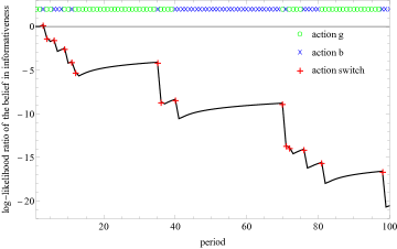
Figure 2.1. This simulation illustrates the log-likelihood ratio of an outside observer’s belief in an informative source compared to an uninformative source over 100 periods. The process is generated under uninformative signals with a normal distribution with mean 0 and variance $2$. The corresponding informative signals are normally distributed with unit variance and mean $-1$ and $+1$, respectively. Red crosses mark the periods in which action switches occur.

We illustrate the aforementioned intuition in Figure 2.1. It depicts a simulation of an outside observer’s belief about the source being informative (in its log-likelihood ratio) under uninformative signals with fatter tails. First, observe that every action switch after an extended period of identical actions leads to a significant decrease in the observer’s belief that the source is informative. As discussed before, observing these unusual action switches makes the observer less convinced that the source is informative. Second, although his belief gradually increases in the absence of action switches, our main result implies that it will eventually converge to zero, so the corresponding log-likelihood ratio will converge to negative infinity. By contrast, if his belief were generated under uninformative signals with thinner tails, then extreme signals would be less likely, and so would be action switches. Consequently, these action switches would eventually cease, and thus his belief would no longer converge to zero.

3. Model

3.1. Setup

There is an unknown binary state of the world $\theta\in\{\mathfrak{g},\mathfrak{b}\}$, chosen at time $0$ with equal probability. We refer to $\mathfrak{g}$ as the good state and $\mathfrak{b}$ as the bad state. A countably infinite set of agents indexed by time $t\in\mathbbm{N}=\{1,2,\ldots\}$ arrive in order, each acting once. The action of agent $t$ is $a_{t}\in A=\{\mathfrak{g},\mathfrak{b}\}$, with a payoff of one if her action matches the state $\theta$ and zero otherwise. Before agent $t$ chooses an action, she observes the history of actions made by her predecessors $H_{t}=(a_{1},\ldots,a_{t-1})$ and receives a private signal $s_{t}$, taking values in a measurable space $(S,\Sigma)$.

A pure strategy of agent $t$ is a measurable function $\sigma_{t}:A^{t-1}\times S\to A$ that selects an action for each possible pair of observed history and private signal. A pure strategy profile $\sigma=(\sigma_{t})_{t\in\mathbbm{N}}$ is a collection of pure strategies of all agents. A strategy profile is a Bayesian Nash equilibrium—referred to as equilibrium hereafter—if no agent can unilaterally deviate from this profile and obtain a strictly higher expected payoff conditioned on their information. Given that each agent acts only once, the existence of an equilibrium is guaranteed by a simple inductive argument. In equilibrium, each agent $t$ chooses the action $a_{t}$ that maximizes her expected payoff given the available information:

$$a_{t}\in\operatorname*{arg\,max}_{a\in A}\mathbb{E}[\mathbbm{1}(\theta=a)|H_{t},s_{t}].$$

Below, we make a continuity assumption which implies that agents are never indifferent, and so there is a unique equilibrium.

3.2. The Informativeness of the Source

So far, the above setup is the canonical setting of the sequential social learning model (Banerjee, 1992; Bikhchandani, Hirshleifer, and Welch, 1992; Smith and Sørensen, 2000). Our model builds on this setting and introduces another dimension of uncertainty regarding the informativeness of a common source. Specifically, at time 0, independent of the payoff-relevant state $\theta$, nature chooses an additional binary state $\omega\in\{0,1\}$ with equal probability. When $\omega=1$, the source is informative and sends i.i.d. signals across agents conditional on $\theta$, with distribution $\mu_{\theta}$. When $\omega=0$, the source is uninformative and still sends i.i.d. signals, but independently of $\theta$, with distribution $\mu_{0}$. The realization of $\omega$ determines the signal-generating process for all agents. Throughout, we denote by $\mathbb{P}_{0}[\cdot]:=\mathbb{P}[\cdot\leavevmode\nobreak\ |\leavevmode\nobreak\ \omega=0]$ and $\mathbb{P}_{1}[\cdot]:=\mathbb{P}[\cdot\leavevmode\nobreak\ |\leavevmode\nobreak\ \omega=1]$ the conditional probability distributions given $\omega=0$ and $\omega=1$, respectively. Similarly, we use the notation $\mathbb{P}_{1,\mathfrak{g}}[\cdot]:=\mathbb{P}[\cdot\leavevmode\nobreak\ |\leavevmode\nobreak\ \omega=1,\theta=\mathfrak{g}]$ to denote the conditional probability distribution given $\omega=1$ and $\theta=\mathfrak{g}$. We use an analogous notation for $\omega=1$ and $\theta=\mathfrak{b}$.

We first observe that, despite the uncertainty regarding the informativeness of the source, in equilibrium, each agent chooses the action that is most likely to match the state, conditional on the source being informative.

Lemma 1.

The equilibrium action for each agent $t$ is

$$a_{t}\in\operatorname*{arg\,max}_{a\in A}\mathbb{P}_{1}[\theta=a|H_{t},s_{t}].$$ (1)

That is, agents always act as if signals are informative, irrespective of the underlying signal-generating process. This lemma holds simply because treating signals as informative—even when they are pure noise—does not adversely affect agents’ payoffs, since in the absence of any useful information, each agent is indifferent between the available actions given the uniform prior assumption.

3.3. Information Structure

The distributions $\mu_{\mathfrak{g}},\mu_{\mathfrak{b}}$, and $\mu_{0}$ are distinct and mutually absolutely continuous, so no signal fully reveals either state $\theta$ or $\omega$. As a consequence, conditioned on $\omega=1$, the log-likelihood ratio of any signal

$$\ell_{t}=\log\frac{d\mu_{\mathfrak{g}}}{d\mu_{\mathfrak{b}}}(s_{t}),$$

is well-defined, and we call it the agent’s private log-likelihood ratio. By Lemma 1, $\ell_{t}$ captures how agents update their private beliefs regarding the relative likelihood of the good state over the bad state upon receiving their signals, regardless of the realization of $\omega$. Hence, it is sufficient to consider $\ell_{t}$ to capture agents’ behavior. We denote by $F_{\mathfrak{g}}$ and $F_{\mathfrak{b}}$ the cumulative distribution functions (CDFs) of $\ell_{t}$ conditioned on the event that $\omega=1$ and $\theta=\mathfrak{g}$ and the event that $\omega=1$ and $\theta=\mathfrak{b}$, respectively. We denote by $F_{0}$ the CDF of $\ell_{t}$ conditioned on $\omega=0$. All conditional CDFs $F_{\mathfrak{g}}$, $F_{\mathfrak{b}}$, and $F_{0}$ are mutually absolutely continuous, as $\mu_{\mathfrak{g}},\mu_{\mathfrak{b}}$ and $\mu_{0}$ are. Let $f_{\mathfrak{g}},f_{\mathfrak{b}}$ and $f_{0}$ denote the corresponding density functions of $F_{\mathfrak{g}}$, $F_{\mathfrak{b}}$ and $F_{0}$ whenever they are differentiable.

We focus on unbounded signals in the sense that the agent’s private log-likelihood ratio can take on arbitrarily large or small values, i.e., for any $M\in\mathbbm{R}$, there exists a positive probability that $\ell_{t}>M$ and a positive probability that $\ell_{t}<-M$. We informally refer to a signal $s_{t}$ as extreme when the corresponding $\ell_{t}$ it induces has a large absolute value. A common example of unbounded private signals is the case of Gaussian signals, where $s_{t}$ follows a normal distribution $\mathcal{N}(m_{(\omega,\theta)},\sigma^{2})$ with variance $\sigma^{2}$ and mean $m_{(\omega,\theta)}$ that depends on the pair of states $(\omega,\theta)$. An extreme Gaussian signal is a signal that is, for example, $5-\sigma$ away from the mean $m_{(\omega,\theta)}$.

We make two assumptions for expository simplicity. First, we assume that the pair $(F_{\mathfrak{g}},F_{\mathfrak{b}})$ of informative conditional CDFs is symmetric around zero, i.e., $F_{\mathfrak{g}}(x)+F_{\mathfrak{b}}(-x)=1$. This implies that our model is invariant with respect to a relabeling of the payoff-relevant state. Second, we assume that all conditional CDFs—$F_{\mathfrak{g}}$, $F_{\mathfrak{b}}$ and $F_{0}$—are continuous, so agents are never indifferent between actions.

In addition, we assume that $F_{\mathfrak{b}}$ has a differentiable left tail, i.e., is differentiable for all $x$ negative enough and its probability density function $f_{\mathfrak{b}}$ satisfies the condition that $f_{\mathfrak{b}}(-x)<1$ for all $x$ large enough. By the symmetry assumption, this implies that $F_{\mathfrak{g}}$ also has a differentiable right tail and its density function $f_{\mathfrak{g}}$ satisfies the condition that $f_{\mathfrak{g}}(x)<1$ for all $x$ large enough. This is a mild technical assumption that holds for every non-atomic distribution commonly used in the literature, including the Gaussian distribution. It holds, for instance, whenever the density tends to zero at infinity.

3.4. Asymptotic Learning

We denote by $q_{t}:=\mathbb{P}[\omega=1|H_{t}]$ the belief that an outside observer assigns to the source being informative after observing the history of agents’ actions from time $1$ to $t-1$. As this observer collects more information over time, his belief $q_{t}$ converges almost surely since it is a bounded martingale. To ensure that he eventually learns the truth regarding the informativeness of the source, we introduce the following notion of asymptotic learning.

Definition 1.

Asymptotic learning holds if for all $\omega\in\{0,1\}$,

$$\lim_{t\to\infty}q_{t}=\omega\quad\mathbb{P}_{\omega}\text{-almost surely.}$$

That is, conditioned on an informative source, the outside observer’s belief that the source is informative converges to one almost surely; meanwhile, conditioned on an uninformative source, his belief that the source is informative converges to zero almost surely. As we explain below in Section 5.1, asymptotic learning is always attainable, regardless of the underlying information structure, when all signals are publicly observable.

4. Relative Tail Thickness

To study the conditions for asymptotic learning, it is crucial to understand the concept of relative tail thickness, which compares the tail distributions of agents’ private log-likelihood ratios induced by different signals. This comparison is important because it captures the relative likelihood of generating extreme signals from different sources. Formally, for any pair of CDFs $(F_{0},F_{\theta})$ where $\theta\in\{\mathfrak{g},\mathfrak{b}\}$ and some $x\in\mathbbm{R}_{+}$, we denote their corresponding ratios by

$$L_{\theta}(x):=\frac{F_{0}(-x)}{F_{\theta}(-x)}\quad\text{and}\quad R_{\theta}(x):=\frac{1-F_{0}(x)}{1-F_{\theta}(x)}.$$

For large $x$, $L_{\theta}(x)$ and $R_{\theta}(x)$ represent the left and right tail ratios of $F_{0}$ over $F_{\theta}$, respectively. The following definitions of fatter and thinner tails describe situations in which extreme signals are either more or less likely to occur under an uninformative source compared to an informative one.

Definition 2.

1. The uninformative signals have fatter tails than the informative signals if there exists $\varepsilon>0$ such that

   $$L_{\mathfrak{b}}(x)\geq\varepsilon\leavevmode\nobreak\ \text{and}\leavevmode\nobreak\ R_{\mathfrak{g}}(x)\geq\varepsilon\quad\text{for all $x$ large enough.}$$

2. The uninformative signals have thinner tails than the informative signals if there exists $\varepsilon>0$ such that either

   $$L_{\mathfrak{g}}(x)\leq 1/\varepsilon\quad\text{for all $x$ large enough,}$$

   or

   $$R_{\mathfrak{b}}(x)\leq 1/\varepsilon\quad\text{for all $x$ large enough.}$$

That is, for the uninformative signals to have fatter tails, both their corresponding left and right tail ratios need to be eventually bounded from below. Conversely, for the uninformative signals to have thinner tails, at least one of their corresponding tail ratios—either left or right—needs to be eventually bounded from above.

Note that the first condition $L_{\mathfrak{b}}(x)\geq\varepsilon$ implies that $L_{\mathfrak{g}}(x)\geq\varepsilon$. This follows from the well-known fact that $F_{\mathfrak{g}}$ exhibits first-order stochastic dominance over $F_{\mathfrak{b}}$, i.e., $F_{\mathfrak{g}}(x)\leq F_{\mathfrak{b}}(x)$ for all $x\in\mathbb{R}$ (see, e.g., Smith and Sørensen, 2000; Chamley, 2004; Rosenberg and Vieille, 2019). Similar statements apply to the remaining three conditions. Furthermore, note that the uninformative signals cannot have fatter and thinner tails simultaneously, as $F_{\mathfrak{g}}$ and $F_{\mathfrak{b}}$ represent distributions of the agent’s private log-likelihood ratio. However, there are distributions under which the uninformative signals have neither fatter nor thinner tails. For these cases, we characterize the conditions for asymptotic learning in the canonical Gaussian environment (see more details in Section 5.3).

Intuitively, compared to informative signals, uninformative signals with fatter tails are more likely to exhibit extreme values. Thus, by Bayes’ Theorem, observing an extreme signal suggests that the source is uninformative. In contrast, uninformative signals with thinner tails tend to exhibit moderate values, so observing an extreme signal in this case suggests that the source is informative. Next, we provide three examples of uninformative signals with either fatter or thinner tails.

Example 1 (Gaussian Signals).

Consider the case where $F_{\mathfrak{g}}$ is normal with mean $+1$ and unit standard deviation and $F_{\mathfrak{b}}$ is also normal with mean $-1$ and unit standard deviation.

Suppose that $F_{0}$ has zero mean. If it has a standard deviation of 17, then the uninformative signals have fatter tails. In this case, if an extreme signal, such as anything above 11, is observed, it is much more likely that the source is uninformative than that an informative $10-\sigma$ signal were generated under $F_{\mathfrak{g}}$. On the other hand, if the standard deviation of $F_{0}$ is $1/17$, then the uninformative signals have thinner tails, and thus an extreme signal indicates that the source is informative. A graphical example of uninformative Gaussian signals with fatter and thinner tails is shown in Figure 4.1.

Figure 4.1. Probability density functions of informative Gaussian signals and their corresponding uninformative Gaussian signals with fatter tails (on the left) and with thinner tails (on the right).

Example 2 (First-Order Stochastically Dominated (FOSD) Signals).

Suppose that $F_{0}$ first-order stochastically dominates $F_{\mathfrak{g}}$. In this case, since the uninformative signals are more likely to exhibit high values, $F_{0}$ has a thinner left tail than $F_{\mathfrak{g}}$, and thus by definition, it has thinner tails than the informative signals.

Now, suppose that an extreme signal of a positive value is observed. Then, it is highly unlikely that the source is informative and associated with the bad state. Instead, it suggests that the source is more likely to be either uninformative or informative but associated with the good state. In this case, even though the observation of an extremely positive signal provides some evidence of the good state, it remains unclear whether the source is informative, as such a signal is likely to occur under both $F_{0}$ and $F_{\mathfrak{g}}$.

Example 3 (Mixture Signals).

For any pair of distributions $(F_{\mathfrak{g}},F_{\mathfrak{b}})$ and any $\alpha\in(0,1)$, let $F_{0}=\alpha F_{\mathfrak{g}}+(1-\alpha)F_{\mathfrak{b}}$. Observe that the uninformative signals represented by $F_{0}$ have fatter tails than the informative signals. In particular, when $\alpha=1/2$, the corresponding mixture distribution $F_{0}=(F_{\mathfrak{g}}+F_{\mathfrak{b}})/2$ coincides with the unconditional distribution of $\ell_{t}$ generated by an informative source. Thus, we can think of this uninformative source as being a priori indistinguishable from the informative one.

Alternatively, the mixture distribution $F_{0}$ can be viewed as generating conditionally i.i.d. signals, but instead of conditioning on the state $\theta$, they are generated conditioned on a different state $\eta$. Specifically, suppose that in each period, the state $\eta$ is randomly drawn from the same set $\{\mathfrak{g},\mathfrak{b}\}$, independent of $\theta$. Say, with probability $\alpha$, the event $\eta=\mathfrak{g}$ occurs and a signal is drawn from the distribution $F_{\mathfrak{g}}$. With the complementary probability, the event $\eta=\mathfrak{b}$ occurs, and a signal is drawn from the distribution $F_{\mathfrak{b}}$.

5. Main Results

5.1. A Benchmark

As a benchmark, we briefly discuss the case where all signals are observed by the outside observer. Depending on the realizations of $\theta$ and $\omega$, these signals are distributed according to either $\mu_{\mathfrak{g}}$, $\mu_{\mathfrak{b}}$ or $\mu_{0}$. Since these measures are distinct, as the sample size grows, this observer eventually learns which distribution is being sampled. Formally, at time $t$, the empirical distribution of the signals $\hat{\mu}_{t}$ assigns to a measurable set $B\subseteq S$ the probability

$$\hat{\mu}_{t}(B):=\frac{1}{t}\sum_{\tau=1}^{t}\mathbbm{1}(s_{\tau}\in B).$$

Conditional on both states $\omega$ and $\theta$, this is the empirical mean of i.i.d. Bernoulli random variables. Hence, by the strong law of large numbers, for every measurable set $B\subseteq S$,

$$\lim_{t\to\infty}\hat{\mu}_{t}(B)=\mu_{(\omega,\theta)}(B)\quad\text{almost surely,}$$

where $\mu_{(1,\mathfrak{g})}=\mu_{\mathfrak{g}}$, $\mu_{(1,\mathfrak{b})}=\mu_{\mathfrak{b}}$ and $\mu_{(\cdot,0)}=\mu_{0}$.

Thus, regardless of the underlying signal-generating process, any uncertainty concerning the informativeness of the source is eventually resolved if all signals are publicly observable. Next, we turn to our main setting where the signals remain private and only the actions are observable. Clearly, in this setting, less information is available—observed actions contain less information than private signals. In addition, one needs to take into account the positive correlation between these observed actions.

5.2. Public Actions

We now present our main result (Theorem 1). In contrast to the public signal benchmark, our main result shows that the achievement of asymptotic learning is no longer guaranteed. In fact, the key determinant of asymptotic learning is the relative tail thickness between the uninformative and informative signals, as introduced in Definition 2.

Theorem 1.

When the uninformative signals have fatter tails than the informative signals, asymptotic learning holds. When the uninformative signals have thinner tails than the informative signals, asymptotic learning fails.

Theorem 1 demonstrates that an outside observer, who learns from observing agents’ actions, eventually distinguishes between informative and uninformative sources if the latter source generates signals with greater dispersion than the former. In contrast, when the uninformative signals are relatively concentrated compared to informative ones, such differentiation becomes unattainable for the observer.

For example, consider informative signals that follow a normal distribution with unit variance and mean $+1$ and $-1$, respectively. When the uninformative signals follow a normal distribution with a variance of 2, they have fatter tails and thus Theorem 1 implies that asymptotic learning holds. In contrast, when the uninformative signals follow a normal distribution with a variance of 1/2, they have thinner tails, and thus Theorem 1 implies that asymptotic learning fails. Indeed, for normal distributions, the relative thickness of the tails is determined solely by their variances: a higher variance corresponds to fatter tails, while a lower variance corresponds to thinner tails (see Lemma 8 in the appendix). An immediate consequence of Theorem 1 is the following result.

Corollary 1.

Suppose all private signals are normal where the informative signals have variance $\sigma^{2}$, and the uninformative signals have variance $\tau^{2}$. Then, asymptotic learning holds if $\tau>\sigma$ and fails if $\tau<\sigma$.

The idea behind our proof of Theorem 1 is as follows. First consider the case where the source is informative. In this case, the likelihood of generating extreme signals that overturn a long streak of correct consensus decreases rapidly. Consequently, agents will eventually reach a consensus on the correct action since they always treat signals as informative. Now, suppose that the source is uninformative and instead of reaching a consensus, agents continue to disagree indefinitely, leading to both actions being taken infinitely often. If this were the case, an outside observer would eventually be able to distinguish between informative and uninformative sources, as they induce distinct behavioral patterns among agents. Whether these disagreements persist or not depends on whether the tails of the uninformative signals are thick enough to generate these overturning extreme signals.

In sum, when the tails of uninformative signals are sufficiently thick (i.e., when they have fatter tails), overturning extreme signals occur often enough so that disagreements persist. When the tails are not sufficiently thick (i.e., when they have thinner tails), these signals are less likely, so disagreements eventually cease. Hence, we conclude that the relative tail thickness between uninformative and informative signals plays an important role in determining the achievement of asymptotic learning.

Perpetual Disagreement

As mentioned above, if agents never reach a consensus under an uninformative source, then intuitively the outside observer can infer the uninformativeness of the source. To formally establish the key mechanism underlying our main result, we define the event in which agents never converge to any action as perpetual disagreement. Let $S:=\sum_{t=1}^{\infty}\mathbbm{1}(a_{t}\neq a_{t+1})$ denote the total number of action switches, so that the event $\{S=\infty\}$ is the perpetual disagreement event. It turns out that perpetual disagreement under an uninformative source is not only a sufficient condition for asymptotic learning but also a necessary condition, as shown in the following proposition.

Proposition 1.

Asymptotic learning holds if and only if conditioned on $\omega=0$, the perpetual disagreement event occurs almost surely.

The proof of Proposition 1 uses the idea of an outside observer whose goal is to guess the informativeness of the source. Note that the achievement of asymptotic learning means that eventually he can always make the correct guess. Since the outsider observes all agents’ actions, he expects to see an eventual consensus when the source is informative. Therefore, if he observes action nonconvergence, he infers that the source must be uninformative and make the correct guess. Conversely, suppose to the contrary that agents could also reach a consensus when the source is uninformative. This implies that action convergence is plausible under both informative and uninformative sources. Consequently, the observer is no longer sure of the source’s informativeness, contradicting our hypothesis that he always makes the correct guess.

5.3. Gaussian Private Signals

While Theorem 1 provides valuable insight into the role of relative tail thickness in determining the achievement of asymptotic learning, there are situations where uninformative signals have neither fatter nor thinner tails compared to informative signals, rendering Theorem 1 inapplicable. For example, consider a scenario where $F_{0}$, $F_{\mathfrak{g}}$, and $F_{\mathfrak{b}}$ are normal distributions with the same variance and mean $0$, $1$, and $-1$, respectively. As $x$ approaches infinity, both $F_{0}(-x)$ and $F_{\mathfrak{b}}(-x)$ approach zero, but the former goes to zero much faster than the latter, leading $L_{\mathfrak{b}}(x)$ converging to zero. As a result, $F_{0}$ does not have fatter tails. Similarly, both $L_{\mathfrak{g}}(x)$ and $R_{\mathfrak{b}}(x)$ tend to infinity as $x$ approaches infinity, so $F_{0}$ does not have thinner tails either.

To complement the findings of Theorem 1, we focus on the Gaussian environment where all signals are normal and share the same variance $\sigma^{2}$. The informative signals are symmetric with mean $+1$ and $-1$, respectively, while the uninformative signals have mean $m_{0}\in(-1,1)$. In this setting, a simple calculation shows that the agent’s private log-likelihood ratio is directly proportional to the private signal: $\ell_{t}=2s_{t}/\sigma^{2}$. As a consequence, all distributions $F_{\mathfrak{g}}$, $F_{\mathfrak{b}}$, and $F_{0}$ are also Gaussian. In the following result, we show that asymptotic learning is achieved if and only if the uninformative signals are symmetric around zero.

Theorem 2.

Suppose all private signals are Gaussian with the same variance, where informative signals have means $-1$ and $+1$, and uninformative signals have mean $m_{0}\in(-1,1)$. Then, asymptotic learning holds if and only if $m_{0}=0$.

Together with Corollary 1, Theorem 2 provides a complete characterization of asymptotic learning in the Gaussian environment with symmetric informative signals. In particular, it shows that in such an environment, asymptotic learning holds in a knife-edge case where the uninformative distribution is symmetric around zero. Intuitively, any deviation in the mean of $F_{0}$ away from zero would bring $F_{0}$ closer to either $F_{\mathfrak{g}}$ or $F_{\mathfrak{b}}$, thus making the uninformative signals more similar to the corresponding informative signals. Consequently, it becomes impossible to fully differentiate between them.

5.4. Numerical Simulation

To further illustrate our main result, we use Monte Carlo simulations to numerically simulate the belief process of an outside observer and the corresponding action switches among agents. We fix the pair of informative Gaussian signal distributions to be $(\mu_{\mathfrak{g}},\mu_{\mathfrak{b}})$ where $\mu_{\mathfrak{g}}=\mathcal{N}(+1,2)$ and $\mu_{\mathfrak{b}}=\mathcal{N}(-1,2)$ and simulate these processes under fatter-tailed uninformative Gaussian signals with distribution $\mu_{0}=\mathcal{N}(0,3)$ and thinner-tailed uninformative Gaussian signals with distribution $\mu_{0}=\mathcal{N}(0,1)$, respectively. We conduct these simulations 1,000 times and calculate the averages for each period. This yields approximations for the expected belief and the expected total number of action switches in the presence of uninformative signals. Figure 5.1 displays the results of these simulations.

Figure 5.1. The belief that the source is informative (on the left) and the total number of action switches (on the right) under uninformative signals with fatter and thinner tails.

What immediately stands out is that under fatter-tailed uninformative signals, the belief of the outside observer that the source is informative decreases much faster compared to thinner-tailed uninformative signals. By period 60, this belief is approximately 0.3 under fatter-tailed uninformative signals, which is less than two-thirds of the belief observed under thinner-tailed uninformative signals. These findings align with the predictions of Theorem 1, suggesting that in the former case the observer will eventually learn that the source is uninformative. In contrast, with thinner-tailed uninformative signals, the decline in the belief about the source’s informativeness plateaus around 0.48 after period 20, suggesting that the observer will not be able to learn that the source is uninformative.

As shown in Proposition 1, the key mechanism driving asymptotic learning is the persistence of disagreements under an uninformative source. Recall that the intuition is that the uninformative source with fatter tails has a higher probability of generating extreme signals, which in turn, prevents agents from converging to a consensus. This phenomenon is evident in the right plot of Figure 5.1, where the average total number of action switches under fatter-tailed uninformative signals increases over time. In contrast, under the thinner-tailed uninformative signals, the total number of switches plateaus in a short amount of time, suggesting that perpetual disagreement does not occur in this case.

6. Asymptotic Learning and Other Notions of Learning

In this section, we discuss the connections between asymptotic learning and other notions of learning that have been studied in the literature. One common notion, concerning the convergence of agents’ actions, is known as herding. Another notion, concerning the convergence of agents’ beliefs, is known as complete learning. We will show that in the presence of information uncertainty, agents may eventually choose the correct action without ever being certain that it is correct.

Formally, we say that correct herding holds if $\lim_{t\to\infty}a_{t}=\theta$ almost surely. That is, the event that all but finitely many agents take the correct action occurs with probability one. Let $p_{t}:=\mathbb{P}[\theta=\mathfrak{g}|H_{t}]$ denote the belief assigned by agent $t$ to the good state given the history of observed actions; we refer to it as the social belief at time $t$. We say that complete learning holds if the social belief $p_{t}$ almost surely converges to one when $\theta=\mathfrak{g}$ and to zero when $\theta=\mathfrak{b}$. Essentially, complete learning means that society eventually becomes confident that they are making the correct choice.

In the standard model where there is no information uncertainty and the source is always informative, Smith and Sørensen (2000) show that correct herding holds if and only if signals are unbounded. In our model, since agents always act as if signals are informative, when the source is indeed informative and generates unbounded signals, correct herding also holds:

$$\lim_{t\to\infty}a_{t}=\theta\quad\mathbb{P}_{1}\text{-almost surely.}$$

That is, given an informative source, agents eventually converge to the correct action, regardless of the achievement of asymptotic learning. By contrast, given an uninformative source, agents are clearly not guaranteed to converge to the correct action; in fact, their actions may or may not converge at all. Indeed, as suggested by Proposition 1, in this case, agents’ actions do not converge if asymptotic learning holds or they may converge to the wrong action if asymptotic learning fails.

Nevertheless, the achievement of correct herding under an informative source does not imply the attainment of complete learning. In this case, although agents eventually converge to the correct action, they remain uncertain about its correctness unless asymptotic learning holds. Conversely, if the informativeness of the source remains uncertain, so do agents’ beliefs about the correctness of their action consensus. We summarize this relationship in the following proposition.

Proposition 2.

Asymptotic learning holds if and only if conditioned on $\omega=1$, complete learning holds.

The proof of Proposition 2 uses the idea of an outside observer who observes the same public information as agent $t$, but does not observe her private signal. So, at time $t$, the observer’s belief is equal to the social belief. As long as the observer remains uncertain about the source’s informativeness, he cannot fully trust the public information, which consists of agents’ actions. Conversely, once the source’s informativeness is confirmed, this public information becomes highly accurate, enabling his belief to converge to the truth. The next result shows that when the source is uninformative, achieving asymptotic learning is equivalent to the social belief converging to the uniform prior.

Proposition 3.

Asymptotic learning holds if and only if conditioned on $\omega=0$, $\lim_{t\to\infty}p_{t}=1/2$ almost surely.

The proof of Proposition 3 uses a similar approach to Proposition 2 and applies the result of Proposition 1. One direction is straightforward: Once an outside observer learns that the source is uninformative, his belief about the payoff-relevant state remains uniform since agents’ actions are based on signals that contain no information. For the other direction, suppose that asymptotic learning fails under an uninformative source. Then, by Proposition 1, it implies that agents may eventually reach a consensus on some action. Since this is also possible under an informative source, the observer cannot completely disregard the possibility that agents’ actions are informative. As a consequence, his belief about the payoff-relevant state is not guaranteed to remain uniform.

7. Analysis

In this section we first examine how agents update their beliefs. We present two standard yet useful properties of their belief updating process, namely, the overturning principle and stationarity. Then, based on Proposition 1, we characterize asymptotic learning in terms of immediate agreement—the event in which all agents immediately reach a consensus on some action—which simplifies the problem of asymptotic learning. Finally, we provide a proof sketch of our main result (Theorem 1) at the end of this section.

7.1. Agents’ Beliefs Dynamics

Since agents always act as if signals are informative (Lemma 1), we focus on how agents update their beliefs conditioned on an informative source. We denote by $\pi_{t}$ the public belief that agent $t$ assigns to the good state after observing the history of actions $H_{t}$, i.e., $\pi_{t}:=\mathbb{P}_{1}[\theta=\mathfrak{g}|H_{t}]$. The corresponding log-likelihood ratio of $\pi_{t}$ is given by:

$$r_{t}:=\log\frac{\pi_{t}}{1-\pi_{t}}=\log\frac{\mathbb{P}_{1}[\theta=\mathfrak{g}|H_{t}]}{\mathbb{P}_{1}[\theta=\mathfrak{b}|H_{t}]}.$$

Furthermore, let $L_{t}$ denote the log-likelihood ratio of the posterior belief that agent $t$ assigns to the good state over the bad state after observing both the history of actions and her private signal:

$$L_{t}:=\log\frac{\mathbb{P}_{1}[\theta=\mathfrak{g}|H_{t},s_{t}]}{\mathbb{P}_{1}[\theta=\mathfrak{b}|H_{t},s_{t}]}.$$

Recall that $\ell_{t}$ is the log-likelihood ratio of agent $t$’s private belief induced by a signal $s_{t}$ conditioned on $\omega=1$. By Bayes’ rule, we can write

$$L_{t}=r_{t}+\ell_{t}.$$

It follows from (1) that, in equilibrium, agent $t$ chooses action $\mathfrak{g}$ if $\ell_{t}\geq-r_{t}$ and action $\mathfrak{b}$ if $\ell_{t}<-r_{t}$. Hence, conditioned on the state $\theta$ and the event that $\omega=1$, the probability that agent $t$ chooses action $\mathfrak{g}$ is $1-F_{\theta}(-r_{t})$ and the probability that she chooses action $\mathfrak{b}$ is $F_{\theta}(-r_{t})$. As a consequence, the agents’ public log-likelihood ratios $(r_{t})$ evolve as follows:

$$r_{t+1}=r_{t}+D_{\mathfrak{g}}(r_{t})\quad\text{if\leavevmode\nobreak\ }a_{t}=\mathfrak{g},$$ (2)

$$r_{t+1}=r_{t}+D_{\mathfrak{b}}(r_{t})\quad\text{if\leavevmode\nobreak\ }a_{t}=\mathfrak{b},$$ (3)

where

$$D_{\mathfrak{g}}(r):=\log\frac{1-F_{\mathfrak{g}}(-r)}{1-F_{\mathfrak{b}}(-r)}\quad\text{and}\quad D_{\mathfrak{b}}(r):=\log\frac{F_{\mathfrak{g}}(-r)}{F_{\mathfrak{b}}(-r)}.$$

Note that $D_{\mathfrak{g}}$ always takes positive values and $D_{\mathfrak{b}}$ always takes negative values as $F_{\mathfrak{g}}$ first-order stochastically dominates $F_{\mathfrak{b}}$.

Overturning Principle and Stationarity

One important property held by the agent’s public belief is known as the overturning principle (Sørensen, 1996; Smith and Sørensen, 2000), which asserts that a single action switch is sufficient to change the verdict of $\pi_{t}$.

Lemma 2 (Overturning Principle).

For each agent $t$, if $a_{t}=\mathfrak{g}$, then $\pi_{t+1}\geq 1/2$. Similarly, if $a_{t}=\mathfrak{b}$, then $\pi_{t+1}\leq 1/2$.

Another important property held by $\pi_{t}$ is stationarity—the value of $\pi_{t}$ captures all past information about the payoff-relevant state, independent of time. This holds in our model because, regardless of the informativeness of the source, agents always update their public log-likelihood ratios according to either (2) or (3). We further write $\mathbb{P}_{\tilde{\omega},\tilde{\theta},\pi}$ to denote the conditional probability distribution given the pair of state realizations ($\tilde{\omega},\tilde{\theta}$) while highlighting the different values of the prior $\pi$.

Lemma 3 (Stationarity).

For any fixed sequence $(b_{\tau})_{\tau=1}^{k}$ of $k$ actions in $\{\mathfrak{g},\mathfrak{b}\}$, any prior $\pi\in(0,1)$ and any pair $(\tilde{\omega},\tilde{\theta})\in\{0,1\}\times\{\mathfrak{g},\mathfrak{b}\}$

$$\mathbb{P}_{\tilde{\omega},\tilde{\theta}}[a_{t+1}=b_{1},\ldots,a_{t+k}=b_{k}|\pi_{t}=\pi]=\mathbb{P}_{\tilde{\omega},\tilde{\theta},\pi}[a_{1}=b_{1},\ldots,a_{k}=b_{k}].$$

This lemma states that regardless of the source’s informativeness, if agent $t$’s public belief is equal to $\pi$, then the probability of observing a sequence $(b_{1},\ldots,b_{k})$ of actions of length $k$ is the same as observing this sequence starting from time $1$, given that the agents’ prior on the payoff-relevant state is $\pi$.

7.2. Asymptotic Learning and Immediate Agreement

In our model, since the agent’s public belief $\pi_{t}$ evolves as in the standard model, it remains a martingale when the source is informative. However, when the source is uninformative, $\pi_{t}$ ceases to be a martingale under the measure $\mathbb{P}_{0}$. Therefore, we need to employ a different analytical approach to understand what ensures asymptotic learning. To do so, we focus on the event $\{a_{1}=a_{2}=\ldots=a\}$ in which all agents immediately reach a consensus on some action $a\in\{\mathfrak{g},\mathfrak{b}\}$. We denote such an event by $\{\bar{a}=a\}$ and refer to it as immediate agreement on action $a$. Note that conditioned on this event, the process of public log-likelihood ratios $(r_{t})$ is deterministic and evolves according to either (2) or (3).

The following lemma shows that conditioned on an informative source, immediate agreement on the wrong action is impossible, whereas immediate agreement on the correct action is possible, at least for some prior. For brevity, we state this result only for the case where $\theta=\mathfrak{g}$. By symmetry, analogous statements hold for $\theta=\mathfrak{b}$.

Lemma 4.

Conditioned on $\omega=1$ and $\theta=\mathfrak{g}$, the following two conditions hold:

1. Immediate agreement on action $\mathfrak{b}$ is impossible.

2. Immediate agreement on action $\mathfrak{g}$ is possible for some prior $\pi\in(0,1)$.

The first part of Lemma 4 holds since, as mentioned before, conditioned on an informative source, all but finitely many agents take the correct action. This immediately implies that agents cannot reach a consensus on the wrong action from the outset. Likewise, the second part of Lemma 4 holds because if agents eventually reach a consensus on the correct action, by stationarity, they can also do so immediately at least for some prior.

Next, we focus on the immediate agreement event conditioned on an uninformative source. Recall that in Proposition 1, we have established the relationship between asymptotic learning and perpetual disagreement. Building on this, we now characterize asymptotic learning in terms of immediate agreement, which is crucial in proving our main result.

Proposition 4.

Asymptotic learning holds if and only if conditioned on $\omega=0$, immediate agreement on any actions is impossible.

This proposition states that achieving asymptotic learning is equivalent to the absence of immediate agreement starting at a uniform prior given an uninformative source. The proof of Proposition 4 utilizes the idea that the agent’s belief updating process is eventually monotonic—a technical property that we establish in Lemma 6 in the appendix. This property ensures that if immediate agreement is impossible for some prior, e.g., the uniform prior, it becomes impossible for all priors. By applying stationarity, this implies that agents cannot reach a consensus on any actions for any priors. Consequently, perpetual disagreement occurs with probability one, and it follows from Proposition 1 that it is equivalent to asymptotic learning.

Therefore, we have reduced the problem of asymptotic learning to determining the possibility of immediate agreement conditioned on an uninformative source, which is much easier to analyze. Specifically, conditioned on the event $\{\bar{a}=\mathfrak{g}\}$, let $r^{\mathfrak{g}}_{t}$ denote the deterministic process of $r_{t}$ based on (2). Recall that agent $t$ chooses $a_{t}=\mathfrak{g}$ if $\ell_{t}\geq-r_{t}$ and $a_{t}=\mathfrak{b}$ otherwise. Consequently, the probability of $\{\bar{a}=\mathfrak{g}\}$ is equal to the probability that $\ell_{t}\geq-r^{\mathfrak{g}}_{t}$ for all $t\geq 1$. Moreover, conditioned on an uninformative source, since private signals are i.i.d., the corresponding private log-likelihood ratios are also i.i.d. Thus, conditioned on $\omega=0$, the probability of immediate agreement on action $\mathfrak{g}$ is

$$\mathbb{P}_{0}[\bar{a}=\mathfrak{g}]=\prod_{t=1}^{\infty}(1-F_{0}(-r^{\mathfrak{g}}_{t})).$$

To determine whether the above probability is positive or zero, by a standard approximation argument, it is equivalent to examining whether the sum of the probabilities of the following events is finite or infinite:

$$\mathbb{P}_{0}[\bar{a}=\mathfrak{g}]>0\leavevmode\nobreak\ (=0)\leavevmode\nobreak\ \Leftrightarrow\leavevmode\nobreak\ \sum_{t=1}^{\infty}F_{0}(-r^{\mathfrak{g}}_{t})<\infty\leavevmode\nobreak\ (=\infty).$$ (4)

By the symmetry of the model, we also have

$$\mathbb{P}_{0}[\bar{a}=\mathfrak{b}]>0\leavevmode\nobreak\ (=0)\leavevmode\nobreak\ \Leftrightarrow\leavevmode\nobreak\ \sum_{t=1}^{\infty}\big{(}1-F_{0}(r^{\mathfrak{g}}_{t})\big{)}<\infty\leavevmode\nobreak\ (=\infty).$$ (5)

In summary, asymptotic learning holds if and only if conditioned on the source being uninformative, the probability of generating extreme signals decreases slowly enough so that both sums in (4) and (5) are infinite. As we discuss below, for uninformative signals with fatter tails, these sums diverge, and for signals with thinner tails, at least one of these sums converges.

7.3. Proof Sketch of Theorem 1

We conclude this section by providing a sketch of the proof of Theorem 1. On the one hand, by part (i) of Lemma 4, the probability of generating extreme signals that match the payoff-relevant state decreases relatively slowly under informative signals. Hence, if the source is uninformative and generates signals with fatter tails, this probability declines even more slowly. Consequently, both the sums in (4) and (5) are infinite, which means that no immediate agreement is possible. Thus, by Proposition 4, asymptotic learning holds. On the other hand, by part (ii) of Lemma 4, the probability of generating extreme signals that mismatch the state decreases relatively fast under informative signals. Hence, if the source is uninformative and generates signals with thinner tails, this probability decreases even more rapidly, at least for some type of extreme signals. Consequently, either the sum in (4) or the sum in (5) (or both) is finite, which means that immediate agreement on some action is possible. Hence, by Proposition 4, asymptotic learning fails.

8. Conclusion

In this paper, we study the sequential social learning problem in the presence of a potentially uninformative source, e.g., an AI recommendation system of unknown quality. We show that achieving asymptotic learning, in which an outside observer eventually discerns the informativeness of the source, is not guaranteed, and it depends on the relationship between the conditional distributions of the private signals. In particular, it hinges on the relative tail distribution between signals: When uninformative signals have fatter tails compared to their informative counterparts, asymptotic learning holds; conversely, when they have thinner tails, asymptotic learning fails. We also characterize the conditions for asymptotic learning in the canonical case of Gaussian private signals, where the relative tail thickness is incomparable.

More generally, our analysis suggests that irregular behavior, such as an action switch (or disagreement) following a prolonged sequence of identical actions, is the driving force behind asymptotic learning. Indeed, contrary to the public-signal benchmark case in which asymptotic learning is always achieved, with private signals, an outside observer can only learn that the source is uninformative from observing these action switches. We show that conditioned on an uninformative source, when action switches accumulate indefinitely (or disagreements occur perpetually), the observer eventually learns the informativeness of the source, and vice versa. We view this characterization of asymptotic learning as the key mechanism behind our main result.

A limitation of our results is that they apply only asymptotically. Our numerical simulations suggest that in the case of uninformative Gaussian signals with fatter tails, the asymptotics can already kick in relatively early in the process. It would be interesting to understand the speed at which an outside observer learns about the informativeness of the source. Another promising extension is to explore varying degrees of informativeness, beyond the extreme cases currently considered in this paper. For example, instead of having either informative or completely uninformative signals, one could have a distribution over the variance of conditionally i.i.d. Gaussian signals and ask whether learning about the payoff-relevant state is achievable. We leave these questions for future research.

Appendix A Proofs

• Recall that in equilibrium, each agent $t$ chooses the action that is most likely to match the state $\theta$ conditioned on the available information $(H_{t},s_{t})$. By Bayes’ rule, the relative likelihood between the good state and the bad state for agent $t$ is

  $$\frac{\mathbb{P}[\theta=\mathfrak{g}|H_{t},s_{t}]}{\mathbb{P}[\theta=\mathfrak{b}|H_{t},s_{t}]}=\frac{\sum_{\tilde{\omega}\in\{0,1\}}\mathbb{P}_{\tilde{\omega}}[\theta=\mathfrak{g}|H_{t},s_{t}]\cdot\mathbb{P}[\omega=\tilde{\omega}|H_{t},s_{t}]}{\sum_{\tilde{\omega}\in\{0,1\}}\mathbb{P}_{\tilde{\omega}}[\theta=\mathfrak{b}|H_{t},s_{t}]\cdot\mathbb{P}[\omega=\tilde{\omega}|H_{t},s_{t}]}.$$

  Note that $\mathbb{P}_{0}[\theta=\mathfrak{g}|H_{t},s_{t}]=\mathbb{P}_{0}[\theta=\mathfrak{g}]$ and $\mathbb{P}_{0}[\theta=\mathfrak{b}|H_{t},s_{t}]=\mathbb{P}_{0}[\theta=\mathfrak{b}]$ as conditioned on $\omega=0$, neither the history $H_{t}$ nor the signal $s_{t}$ contains any information about the payoff-relevant state $\theta$. Since the states $\omega$ and $\theta$ are independent of each other and the prior on $\theta$ is uniform, $\mathbb{P}_{0}[\theta=\mathfrak{g}|H_{t},s_{t}]=\mathbb{P}_{0}[\theta=\mathfrak{b}|H_{t},s_{t}]=1/2$. Thus, it follows from the above equation that

  $$\frac{\mathbb{P}[\theta=\mathfrak{g}|H_{t},s_{t}]}{\mathbb{P}[\theta=\mathfrak{b}|H_{t},s_{t}]}\geq 1\Leftrightarrow\frac{\mathbb{P}_{1}[\theta=\mathfrak{g}|H_{t},s_{t}]}{\mathbb{P}_{1}[\theta=\mathfrak{b}|H_{t},s_{t}]}\geq 1.$$

  That is, in equilibrium, each agent chooses the most likely action conditioned on the available information and the source being informative. ∎

• For any $t\geq 1$, one has that

  $$\pi_{t+1}=\mathbb{E}_{1}[\mathbbm{1}(\theta=\mathfrak{g})|H_{t+1}]=\mathbb{E}_{1}[\mathbb{E}_{1}[\mathbbm{1}(\theta=\mathfrak{g})|H_{t},s_{t}]|H_{t+1}]],$$

  where the second equality follows from the law of the iterated expectation. Thus, if $a_{t}=\mathfrak{g}$, by Lemma 1, $\mathbb{P}_{1}[\theta=\mathfrak{g}|H_{t},s_{t}]\geq\mathbb{P}_{1}[\theta=\mathfrak{b}|H_{t},s_{t}]$. It follows from the above equation that $\pi_{t+1}\geq 1-\pi_{t+1}$, which implies that $\pi_{t+1}\geq 1/2$. The case where $a_{t}=\mathfrak{b}$ implies that $\pi_{t+1}\leq 1/2$ follows from a symmetric argument. ∎

The following simple claim will be useful in proving Proposition 1. It employs an idea similar to the no introspection principle in Sørensen (1996). Recall that $q_{t}=\mathbb{P}[\omega=1|H_{t}]$ is the belief that an outside observer assigns to the source being informative based on the history of actions from time 1 to $t-1$.

Claim 1.

For any $a\in(0,1/2)$ and any $b\in(1/2,1)$,

$$\mathbb{P}_{0}[q_{t}=\tilde{q}] \leq\frac{1-a}{a}\cdot\mathbb{P}_{1}[q_{t}=\tilde{q}],\text{\leavevmode\nobreak\ for all\leavevmode\nobreak\ }\tilde{q}\in[a,1/2];$$

$$\mathbb{P}_{0}[q_{t}=\tilde{q}] \geq\frac{1-b}{b}\cdot\mathbb{P}_{1}[q_{t}=\tilde{q}],\text{\leavevmode\nobreak\ for all\leavevmode\nobreak\ }\tilde{q}\in[1/2,b].$$

• For any $\tilde{q}\in(0,1)$, let $\tilde{H}_{t}$ be a history of actions such that the associated belief $q_{t}$ is equal to $\tilde{q}$. By the law of total expectation,

  $$\mathbb{P}[\omega=1|q_{t}=\tilde{q}] =\mathbb{E}[\mathbb{E}[\mathbbm{1}(\omega=1)|\tilde{H}_{t}]|q_{t}=\tilde{q}]=\mathbb{E}[\tilde{q}|q_{t}=\tilde{q}]=\tilde{q}.$$

  It follows from Bayes’ rule that

  $$\frac{\mathbb{P}_{0}[q_{t}=\tilde{q}]}{\mathbb{P}_{1}[q_{t}=\tilde{q}]}=\frac{\mathbb{P}[\omega=0|q_{t}=\tilde{q}]}{\mathbb{P}[\omega=1|q_{t}=\tilde{q}]}\cdot\frac{\mathbb{P}[\omega=1]}{\mathbb{P}[\omega=0]}=\frac{1-\tilde{q}}{\tilde{q}}.$$

  Since for any $a\in(0,1/2)$ and any $\tilde{q}\in[a,1/2]$, $1\leq\frac{1-\tilde{q}}{\tilde{q}}\leq\frac{1-a}{a}$, it follows from the above equation that

  $$\mathbb{P}_{0}[q_{t}=\tilde{q}]=\frac{1-\tilde{q}}{\tilde{q}}\cdot\mathbb{P}_{1}[q_{t}=\tilde{q}]\leq\frac{1-a}{a}\cdot\mathbb{P}_{1}[q_{t}=\tilde{q}].$$

  The second inequality follows from an identical argument. ∎

In the following proofs for Proposition 1, 2 and 3, we use extensively the idea of an outside observer, say observer $x$, who observes everyone’s actions. The information available to him at time $t$ is thus $H_{t}=(a_{1},\ldots,a_{t-1})$ and at time infinity is $H_{\infty}=\cup_{t}H_{t}$. He gets a utility of one if his guess about $\omega$ is correct and zero otherwise. Furthermore, we denote by $q_{\infty}:=\mathbb{P}[\omega=1|H_{\infty}]$ the belief that he has at time infinity about the event $\omega=1$. Similarly, we denote by $p_{\infty}:=\mathbb{P}[\theta=\mathfrak{g}|H_{\infty}]$ the belief that he has at time infinity about the event $\theta=\mathfrak{g}$.

• We first show the if direction. Recall that $S=\sum_{t=1}^{\infty}\mathbbm{1}(a_{t}\neq a_{t+1})$ and suppose that $\mathbb{P}_{0}[S=\infty]=1$. Denote by $a^{x}_{t}$ the guess that the outside observer $x$ would make to maximize his probability of guessing $\omega$ correctly at time $t$. Fix a large positive integer $k\in\mathbbm{N}$. Let $A_{t}(k)$ denote the event that there have been at least $k$ action switches before time $t$ and denote its complementary event by $A^{c}_{t}(k)$.

  Consider the following strategy $\tilde{a}^{x}_{\infty}(k)$ for $x$ at time infinity: $\tilde{a}^{x}_{\infty}(k)=0$ if $A_{\infty}(k)$ occurs and $\tilde{a}^{x}_{\infty}(k)=1$ otherwise. That is, the observer would guess $0$ if there are at least $k$ action switches at time infinity and guess $1$ otherwise. The expected payoff of $x$ under this strategy is

  $$\mathbb{P}[\tilde{a}^{x}_{\infty}(k)=\omega]=\mathbb{P}_{0}[A_{\infty}(k)]\cdot\mathbb{P}[\omega=0]+\mathbb{P}_{1}[A^{c}_{\infty}(k)]\cdot\mathbb{P}[\omega=1].$$ (A.1)

  Since conditioned on $\omega=1$, agents eventually reach a consensus almost surely, it follows that for all $k$ large enough,

  $$\mathbb{P}_{1}[A^{c}_{\infty}(k)]=1.$$ (A.2)

  By assumption, $\mathbb{P}_{0}[S=\infty]=1$, which implies that $\mathbb{P}_{0}[A_{\infty}(k)]=1$ for all $k$. Thus, it follows from (A.1) and (A.2) that for all $k$ large enough, $\mathbb{P}[\tilde{a}^{x}_{\infty}(k)=\omega]=1$. In other words, for all $k$ large enough, the strategy $\tilde{a}^{x}_{\infty}(k)$ achieves the maximal payoff for $x$.

  Meanwhile, note that the optimal strategy for $x$ at time infinity is to make a guess that he believes is most likely, given the information $H_{\infty}$: $a^{x}_{\infty}=1$ if $q_{\infty}\geq 1/2$ and $a^{x}_{\infty}=0$ otherwise. Since $\mathbb{P}[\tilde{a}_{\infty}^{x}(k)=\omega]=1$ for all $k$ large enough, the optimal strategy $a^{x}_{\infty}$ must also achieve the maximal payoff of one:

  $$1=\mathbb{P}[a^{x}_{\infty}=\omega]=\mathbb{P}_{1}[q_{\infty}\geq 1/2]\cdot\mathbb{P}[\omega=1]+\mathbb{P}_{0}[q_{\infty}<1/2]\cdot\mathbb{P}[\omega=0].$$ (A.3)

  It follows from (A.3) that $\mathbb{P}_{0}[q_{\infty}<1/2]=\mathbb{P}_{1}[q_{\infty}\geq 1/2]=1$. It remains to show that $\mathbb{P}_{0}[q_{\infty}=0]=1$ and $\mathbb{P}_{1}[q_{\infty}=1]=1$. To this end, first notice that $\mathbb{P}_{0}[q_{\infty}<1/2]=1$ implies that $\mathbb{P}_{0}[q_{\infty}\geq 1/2]=0$. Thus, by Claim 1, it further implies that for any $b\in(1/2,1)$ and all $\tilde{q}\in[1/2,b]$, $\mathbb{P}_{1}[q_{\infty}=\tilde{q}]=0$. Consequently, it follows from $\mathbb{P}_{1}[q_{\infty}\geq 1/2]=1$ that $\mathbb{P}_{1}[q_{\infty}=1]=1$. The case that $\mathbb{P}_{0}[q_{\infty}=0]=1$ follows from an identical argument. Together, we conclude that asymptotic learning holds.

Next, we show the only-if direction. Suppose by contraposition that $\mathbb{P}_{0}[S<\infty]>0$. Again, since conditioned on $\omega=1$, agents eventually reach a consensus on the correct action, this implies that $\mathbb{P}_{1}[S<\infty]=1$. Thus, there exists a history of actions $\tilde{H}_{\infty}$ at time infinity that is possible under both probability measures $\mathbb{P}_{0}$ and $\mathbb{P}_{1}$: $\mathbb{P}_{0}[\tilde{H}_{\infty}]>0$ and $\mathbb{P}_{1}[\tilde{H}_{\infty}]>0$. It follows from Bayes’ rule that $\mathbb{P}[\omega=1|\tilde{H}_{\infty}]<1$ and $\mathbb{P}[\omega=0|\tilde{H}_{\infty}]<1$.

Assume without loss of generality that under this history $\tilde{H}_{\infty}$, the corresponding belief $\tilde{q}_{\infty}\geq 1/2$. Therefore, given $\tilde{H}_{\infty}$, the observer $x$ would guess $a^{x}_{\infty}=1$. As a consequence, the probability of $x$ guessing correctly about $\omega$ is strictly less than one:

$$\mathbb{P}[a^{x}_{\infty}=\omega] =\mathbb{P}[a^{x}_{\infty}=\omega,\tilde{H}_{\infty}]+\mathbb{P}[a^{x}_{\infty}=\omega,\tilde{H}^{c}_{\infty}]$$

$$=\mathbb{P}[\omega=1|\tilde{H}_{\infty}]\cdot\mathbb{P}[\tilde{H}_{\infty}]+\mathbb{P}[a^{x}_{\infty}=\omega,\tilde{H}^{c}_{\infty}]$$

$$<\mathbb{P}[\tilde{H}_{\infty}]+\mathbb{P}[\tilde{H}^{c}_{\infty}]=1.$$

This implies that asymptotic learning fails since otherwise, by definition $\mathbb{P}[a^{x}_{\infty}=\omega]=1$, which is in contradiction with the above strict inequality. ∎

The following equation will be useful in proving Proposition 2 and 3. Recall that $q_{\infty}$ and $p_{\infty}$ are the beliefs of the observer $x$ assigned to the events $\omega=1$ and $\theta=\mathfrak{g}$ at time infinity, respectively. Denote by $\pi_{\infty}=\mathbb{P}_{1}[\theta=\mathfrak{g}|H_{\infty}]$. By the law of total probability,

$$p_{\infty} =\mathbb{P}_{1}[\theta=\mathfrak{g}|H_{\infty}]\cdot q_{\infty}+\mathbb{P}_{0}[\theta=\mathfrak{g}|H_{\infty}]\cdot(1-q_{\infty})$$

$$=\pi_{\infty}\cdot q_{\infty}+\frac{1}{2}\cdot(1-q_{\infty}),$$ (A.4)

where the second equality holds since conditioned on $\omega=0$, no action contains any information about $\theta$. Thus $\mathbb{P}_{0}[\theta=\mathfrak{g}|H_{\infty}]=\mathbb{P}_{0}[\theta=\mathfrak{g}]=1/2$ given the uniform prior.

• Since agents always act as if signals are informative (Lemma 1), the agent’s public belief $\pi_{t}=\mathbb{P}_{1}[\theta=\mathfrak{g}|H_{t}]$ remains a martingale under the measure $\mathbb{P}_{1}$. Using a standard martingale convergence argument with unbounded signals (Smith and Sørensen, 2000), we have that (i) conditioned on $\omega=1$ and $\theta=\mathfrak{g}$, $\pi_{\infty}=1$ almost surely and (ii) conditioned on $\omega=1$ and $\theta=\mathfrak{b}$, $\pi_{\infty}=0$ almost surely.

  Suppose that conditioned on $\omega=1$, complete learning holds. That is, (i) conditioned on $\omega=1$ and $\theta=\mathfrak{g}$, $p_{\infty}=1$ almost surely and (ii) conditioned on $\omega=1$ and $\theta=\mathfrak{b}$, $p_{\infty}=0$ almost surely. It follows from (A) that conditioned on $\omega=1$, $q_{\infty}=1$ almost surely so that asymptotic learning holds. Conversely, suppose asymptotic learning holds. By definition, conditioned on $\omega=1$, $q_{\infty}=1$ almost surely. It then follows from (A) that conditioned on $\omega=1$, $p_{\infty}=\pi_{\infty}$ almost surely, and thus complete learning holds. ∎

• The only-if direction is straightforward: Suppose asymptotic learning holds. By definition, conditioned on $\omega=0$, $q_{\infty}=0$ almost surely, and thus it follows from (A) that $p_{\infty}=1/2$ almost surely.

  Now, we prove the if direction. Suppose asymptotic learning fails. By Proposition 1, conditioned on $\omega=0$, there exists a history $\tilde{H}_{\infty}$ that is possible at time infinity in which agents eventually reach a consensus on some action. Since such history is also possible conditioned on $\omega=1$, the corresponding belief of an outside observer $\tilde{q}_{\infty}\in(0,1)$. Furthermore, note that depending on the action to which the history $\tilde{H}_{\infty}$ converges, the corresponding public belief of the agent $\tilde{\pi}_{\infty}$ takes values in $\{0,1\}$. Hence, by (A), the event $\{p_{\infty}\neq 1/2\}$ occurs with positive probability. ∎

• The proof idea is similar to the proof of Lemma 10 in Arieli, Babichenko, Müller, Pourbabaee, and Tamuz (2023). Recall that we use $\mathbb{P}_{1,\mathfrak{g}}$ to denote the conditional probability distribution given $\omega=1$ and $\theta=\mathfrak{g}$ and we use $\mathbb{P}_{1,\mathfrak{g},\pi}$ to denote the same conditional probability distribution while emphasizing the prior value. Since conditioned on $\omega=1$, correct herding holds, this means that $\mathbb{P}_{1,\mathfrak{g}}[\lim_{t}a_{t}=\mathfrak{g}]=1$. As a consequence, part (i) follows directly from the fact that the events $\{\bar{a}=\mathfrak{b}\}$ and $\{\lim_{t}a_{t}=\mathfrak{g}\}$ are disjoint, and thus $\mathbb{P}_{1,\mathfrak{g}}[\bar{a}=\mathfrak{b}]=0$.

  For part (ii), let $\tau<\infty$ denote the last random time at which the agent chooses the wrong action $\mathfrak{b}$. It is well-defined as correct herding holds. Hence, $1=\mathbb{P}_{1,\mathfrak{g}}[\lim_{t}a_{t}=\mathfrak{g}]=\sum_{k=1}^{\infty}\mathbb{P}_{1,\mathfrak{g}}[\tau=k]$. By the overturning principle (Lemma 2), $a_{\tau}=\mathfrak{b}$ implies that $\pi_{\tau+1}\leq 1/2$. As a consequence,

  $$1=\sum_{k=1}^{\infty}\mathbb{P}_{1,\mathfrak{g}}[\tau=k] =\sum_{k=1}^{\infty}\mathbb{P}_{1,\mathfrak{g}}[a_{k+1}=a_{k+2}=\ldots=\mathfrak{g},\pi_{k+1}\leq 1/2]$$

  $$=\sum_{k=1}^{\infty}\mathbb{E}_{1,\mathfrak{g}}\big{[}\mathbb{P}_{1,\mathfrak{g}}[a_{k+1}=a_{k+2}=\ldots=\mathfrak{g},\pi_{k+1}\leq 1/2\leavevmode\nobreak\ |\leavevmode\nobreak\ \pi_{k+1}]\big{]}$$

  $$=\sum_{k=1}^{\infty}\mathbb{E}_{1,\mathfrak{g}}\big{[}\mathbbm{1}(\pi_{k+1}\leq 1/2)\cdot\mathbb{P}_{1,\mathfrak{g}}[a_{k+1}=a_{k+2}=\ldots=\mathfrak{g}\leavevmode\nobreak\ |\leavevmode\nobreak\ \pi_{k+1}]\big{]}$$

  $$=\sum_{k=1}^{\infty}\mathbb{E}_{1,\mathfrak{g}}\big{[}\mathbbm{1}(\pi_{k+1}\leq 1/2)\cdot\mathbb{P}_{1,\mathfrak{g},\pi_{k+1}}[\bar{a}=\mathfrak{g}]\big{]},$$

  where the second equality follows from the law of total expectation, and the last equality follows from the stationarity property (Lemma 3). Suppose that for all prior $\pi\in(0,1)$, $\mathbb{P}_{1,\mathfrak{g},\pi}[\bar{a}=\mathfrak{g}]=0$. This implies that the above equation equals zero, a contradiction. ∎

A.1. Proof of Theorem 1

In this section, we prove Proposition 4 and Theorem 1. To prove Proposition 4, we will first prove the following proposition (Proposition 5). Together with Proposition 1, they jointly imply Proposition 4. The proof of Theorem 1 is presented at the end of this section. We write $\mathbb{P}_{0,\pi}$ to denote the conditional probability distribution given $\omega=0$ while highlighting the value of the prior $\pi$ on $\theta$.

Proposition 5.

The following are equivalent.

1. For any action $a\in\{\mathfrak{g},\mathfrak{b}\}$, $\mathbb{P}_{0,\pi}[\bar{a}=a]=0$ for all prior $\pi\in(0,1)$.

2. $\mathbb{P}_{0}[S=\infty]=1$.

3. For any action $a\in\{\mathfrak{g},\mathfrak{b}\}$, $\mathbb{P}_{0,\pi}[\bar{a}=a]=0$ for some prior $\pi\in(0,1)$.

To prove this proposition, we first establish some preliminary results on the process of the agents’ public log-likelihood ratios conditioned on the event of immediate agreement. These results lead to Lemma 7, a crucial part in establishing the equivalence between no immediate agreement and perpetual disagreement conditioned on an uninformative source. We present the proof of Proposition 5 towards the end of this section.

Preliminaries

Recall that conditioned on $\{\bar{a}=\mathfrak{g}\}$, the process of the agent’s public log-likelihood ratio $r_{t}$ evolves deterministically according to $\eqref{eq:highaction}$, which we denote by $r^{\mathfrak{g}}_{t}$. Let the corresponding updating function be

$$\phi(x):=x+D_{\mathfrak{g}}(x).$$

That is, $r^{\mathfrak{g}}_{t+1}=\phi(r^{\mathfrak{g}}_{t})$ for all $t\geq 1$. Since the entire sequence $(r^{\mathfrak{g}}_{t})$ is determined once its initial value $r_{1}^{\mathfrak{g}}$ is specified, we denote the value of $r^{\mathfrak{g}}_{t}$ with an initial value $r_{1}^{\mathfrak{g}}=r$ by $r^{\mathfrak{g}}_{t}(r)$. We can thus write $r^{\mathfrak{g}}_{t}(r)=\phi^{t-1}(r)$ for all $t\geq 1$, where $\phi^{t}$ is its $t$-th composition and $\phi^{0}(r)=r$.

We remind the readers of two standard properties of the sequence $(r^{\mathfrak{g}}_{t})$, as summarized in the following lemma. The first part of this lemma states that $(r^{\mathfrak{g}}_{t})$ tends to infinity as $t$ tends to infinity, and the second part shows that it takes only some bounded time for the sequence $(r^{\mathfrak{g}}_{t})$ to reach any positive value.

Lemma 5 (The Long-Run and Short-Run Behaviors of $r^{\mathfrak{g}}_{t}$).

1. $\lim_{t\to\infty}r^{\mathfrak{g}}_{t}=\infty$.

2. For any $\bar{r}\geq 0$, there exists $t_{0}$ such that $r^{\mathfrak{g}}_{t_{0}}(r)\geq\bar{r}$ for all $r\geq 0$.

• See Lemma 6 and Lemma 12 in Rosenberg and Vieille (2019). ∎

Note that although the sequence $(r^{\mathfrak{g}}_{t})$ eventually approaches infinity, it may not do so monotonically without additional assumptions on the distributions $F_{\mathfrak{g}}$ and $F_{\mathfrak{b}}$. The next lemma shows that, under some mild technical assumptions on the left tail of $F_{\mathfrak{b}}$, the function $\phi(x)$ eventually increases monotonically.

Lemma 6 (Eventual Monotonicity).

Suppose that $F_{\mathfrak{b}}$ has a differentiable left tail and its probability density function $f_{\mathfrak{b}}$ satisfies the condition that, for all $x$ large enough, $f_{\mathfrak{b}}(-x)<1$. Then, $\phi(x):=x+D_{\mathfrak{g}}(x)$ increases monotonically for all $x$ large enough.

• By assumption, we can find a constant $\rho<1$ such that for all $x$ large enough, $f_{\mathfrak{b}}(-x)\leq\rho$. By definition, $D_{g}(x)=\log\frac{1-F_{\mathfrak{g}}(-x)}{1-F_{\mathfrak{b}}(-x)}$. Taking the derivative of $D_{\mathfrak{g}}$,

  $$D_{\mathfrak{g}}^{\prime}(x)=\frac{f_{\mathfrak{g}}(-x)}{1-F_{\mathfrak{g}}(-x)}-\frac{f_{\mathfrak{b}}(-x)}{1-F_{\mathfrak{b}}(-x)}.$$

  Observe that the log-likelihood ratio of the agent’s private log-likelihood ratio $\ell_{t}$ is the log-likelihood ratio itself (see, e.g., Chamley (2004)):

  $$\log\frac{dF_{\mathfrak{g}}}{dF_{\mathfrak{b}}}(x)=x.$$

  It follows that

  $$-D^{\prime}_{\mathfrak{g}}(x)=f_{\mathfrak{b}}(-x)\Big{(}\frac{1}{1-F_{\mathfrak{b}}(-x)}-\frac{\mathrm{e}^{-x}}{1-F_{\mathfrak{g}}(-x)}\Big{)}\leq\frac{f_{\mathfrak{b}}(-x)}{1-F_{\mathfrak{b}}(-x)}.$$

  Fix some $\varepsilon>0$ small enough so that $(1+\varepsilon)\rho\leq 1$. It follows from the above inequality that there exists some $x$ large enough such that $-D^{\prime}_{\mathfrak{g}}(x)\leq(1+\varepsilon)f_{\mathfrak{b}}(-x)$. Furthermore, for all $x^{\prime}\geq x$,

  $$D_{\mathfrak{g}}(x) =D_{\mathfrak{g}}(x^{\prime})-\int_{x}^{x^{\prime}}D^{\prime}_{\mathfrak{g}}(y)dy$$

  $$\leq D_{\mathfrak{g}}(x^{\prime})+(1+\varepsilon)\int_{x}^{x^{\prime}}f_{\mathfrak{b}}(-x)dx$$

  $$=D_{\mathfrak{g}}(x^{\prime})-(1+\varepsilon)(F_{\mathfrak{b}}(-x^{\prime})-F_{\mathfrak{b}}(-x)).$$

  Rearranging the above equation,

  $$D_{\mathfrak{g}}(x)-D_{\mathfrak{g}}(x^{\prime}) \leq(1+\varepsilon)(F_{\mathfrak{b}}(-x)-F_{\mathfrak{b}}(-x^{\prime}))$$

  $$\leq(1+\varepsilon)\rho(x^{\prime}-x),$$

  where the second last inequality follows from the fact that $f_{\mathfrak{b}}(-x)\leq\rho<1$. Since $(1+\varepsilon)\rho\leq 1$, the above inequality implies that there exists some $x$ large enough such that $D_{\mathfrak{g}}(x)+x\leq D_{\mathfrak{g}}(x^{\prime})+x^{\prime}$ for all $x^{\prime}\geq x$. That is, $\phi(x)$ eventually increases monotonically. ∎

Given these lemmas, we are ready to prove the following result. It shows that conditioned on an uninformative source, the possibility of immediate agreement is independent of the prior belief.

Lemma 7.

For any action $a\in\{\mathfrak{g},\mathfrak{b}\}$, the following statements are equivalent:

1. $\mathbb{P}_{0,\pi}[\bar{a}=a]>0$, for some prior $\pi\in(0,1)$;

2. $\mathbb{P}_{0,\pi}[\bar{a}=a]>0$, for all prior $\pi\in(0,1)$.

• The second implication, namely, $(ii)\Rightarrow(i)$ is immediate. We will show the first implication, $(i)\Rightarrow(ii)$. Fix some prior $\tilde{\pi}\in(0,1)$ such that $\mathbb{P}_{0,\tilde{\pi}}[\bar{a}=\mathfrak{g}]>0$ and let $\tilde{r}=\log\frac{\tilde{\pi}}{1-\tilde{\pi}}$. Since $r^{\mathfrak{g}}_{t}(\tilde{r})$ is a deterministic process, the event $\{\bar{a}=\mathfrak{g}\}$ initiated at the prior $\pi_{1}=\tilde{\pi}$ is equivalent to the event $\{\ell_{t}\geq-r^{\mathfrak{g}}_{t}(\tilde{r}),\forall t\geq 1\}$. Conditioned on $\omega=0$, since signals are i.i.d., so are the agents’ private log-likelihood ratios. Thus, we have

  $$\mathbb{P}_{0,\tilde{\pi}}[\bar{a}=\mathfrak{g}] =\prod_{t=1}^{\infty}(1-F_{0}(-r^{\mathfrak{g}}_{t}(\tilde{r})).$$ (A.5)

  As a consequence, $\mathbb{P}_{0,\tilde{\pi}}[\bar{a}=\mathfrak{g}]>0$ if and only if there exists $M<\infty$ such that

  $$-\sum_{t=1}^{\infty}\log\big{(}1-F_{0}(-r^{\mathfrak{g}}_{t}(\tilde{r}))\big{)}<M.$$

  For two sequences $(a_{t})$ and $(b_{t})$, we write $a_{t}\approx b_{t}$ if $\lim_{t\to\infty}(a_{t}/b_{t})=1$. Since $r^{\mathfrak{g}}_{t}(\tilde{r})\to\infty$ (this follows from part (i) of Lemma 5), $\log\big{(}1-F_{0}(-r^{\mathfrak{g}}_{t}(\tilde{r}))\big{)}\approx-F_{0}(-r^{\mathfrak{g}}_{t}(\tilde{r}))$. Thus, the above sum is finite if and only if

  $$\sum_{t=1}^{\infty}F_{0}(-r^{\mathfrak{g}}_{t}(\tilde{r}))<M.$$ (A.6)

  By the overturning principle (Lemma 2), it suffices to show that (A.6) implies that

  $$\sum_{t=1}^{\infty}F_{0}(-r^{\mathfrak{g}}_{t}(r))<M,\quad\text{for any\leavevmode\nobreak\ }r\geq 0.$$

  By the eventual monotonicity of $\phi$ (Lemma 6) and the fact that $r^{\mathfrak{g}}_{t}(\tilde{r})\to\infty$, we can find a large enough $\bar{t}$ such that $r^{\mathfrak{g}}_{\bar{t}}(\tilde{r}):=\bar{r}\geq 0$ and $\phi(r)\geq\phi(\bar{r})$ for all $r\geq\bar{r}$. By part (ii) of Lemma 5, there exists $t_{0}\in\mathbbm{N}$ such that $r^{\mathfrak{g}}_{t_{0}}(r)\geq\bar{r}$ for all $r\geq 0$. Since above $\bar{r}$, $\phi$ is monotonically increasing, one has $\phi(r^{\mathfrak{g}}_{t_{0}}(r))\geq\phi(\bar{r})$ for any $r\geq 0$. Consequently, for all $\tau\geq 1$, $r^{\mathfrak{g}}_{\tau+t_{0}}(r)=\phi^{\tau}(r^{\mathfrak{g}}_{t_{0}}(r))\geq\phi^{\tau}(\bar{r})=r^{\mathfrak{g}}_{\tau+1}(\bar{r})$. Since $r^{\mathfrak{g}}_{\tau+1}(\bar{r})=r^{\mathfrak{g}}_{\tau+1}(r^{\mathfrak{g}}_{\bar{t}}(\tilde{r}))=r^{\mathfrak{g}}_{\tau+\bar{t}}(\tilde{r})$, it follows that

  $$F_{0}(-r^{\mathfrak{g}}_{\tau+t_{0}}(r))\leq F_{0}(-r^{\mathfrak{g}}_{\tau+\bar{t}}(\tilde{r})).$$

  Thus, it follows from (A.6) that for any $r\geq 0$, $\sum_{t=1}^{\infty}F_{0}(-r^{\mathfrak{g}}_{t}(r))<\infty$, as required. The case for action $\mathfrak{b}$ follows from a symmetric argument. ∎

Now, we are ready to prove Proposition 5.

• We show that $(i)\Rightarrow(ii)$, $(ii)\Rightarrow(iii)$, and $(iii)\Rightarrow(i)$. To show the first implication, we prove the contrapositive statement. Suppose that $\mathbb{P}_{0}[S<\infty]>0$. This implies that there exists a sequence of action realizations $(b_{1},b_{2},\ldots,b_{k-1},b_{k}=\ldots=a)$ for some action $a\in\{\mathfrak{b},\mathfrak{g}\}$ such that

  $$\mathbb{P}_{0}[a_{t}=b_{t},\forall t\geq 1]>0.$$

  By stationarity, there exists some $\pi^{\prime}\in(0,1)$ such that

  $$\mathbb{P}_{0,\pi^{\prime}}[\bar{a}=a]>0,$$

  which contradicts (i).

  To show the second implication, suppose towards a contradiction that there exists some action $a\in\{\mathfrak{g},\mathfrak{b}\}$ such that $\mathbb{P}_{0,\pi}[\bar{a}=a]>0$ for all prior $\pi\in(0,1)$. In particular, it holds for the uniform prior. Since the event $\{\bar{a}=a\}$ is contained in the event $\{S<\infty\}$,

  $$0<\mathbb{P}_{0}[\bar{a}=a]\leq\mathbb{P}_{0}[S<\infty].$$

  This implies that $\mathbb{P}_{0}[S=\infty]<1$, a contradiction to (ii).

  Finally, we show the last implication by contraposition. Suppose that there exists some $a\in\{\mathfrak{g},\mathfrak{b}\}$ such that $\mathbb{P}_{0,\pi}[\bar{a}=a]>0$ for some prior $\pi\in(0,1)$. By Lemma 7, it also holds for all prior $\pi\in(0,1)$, which is a contradiction to (iii). This concludes the proof of Proposition 5. ∎

• By the equivalence between (ii) and (iii) in Proposition 5 and Proposition 1, we have shown Proposition 4. ∎

Given Proposition 4, we are now ready to prove our main result.

• By part (i) of Lemma 4, $\mathbb{P}_{1,\mathfrak{b}}[\bar{a}=\mathfrak{g}]=0$ and $\mathbb{P}_{1,\mathfrak{g}}[\bar{a}=\mathfrak{b}]=0$. Following a similar argument that led to (A.5), one has

  $$0=\mathbb{P}_{1,\mathfrak{b}}[\bar{a}=\mathfrak{g}]=\prod_{t=1}^{\infty}(1-F_{\mathfrak{b}}(-r^{\mathfrak{g}}_{t})).$$

  Taking the logarithm on both sides, the above equation is equivalent to $-\sum_{t=1}^{\infty}\log(1-F_{\mathfrak{b}}(-r^{\mathfrak{g}}_{t}))=\infty$. Since $r^{\mathfrak{g}}_{t}\to\infty$, $\log(1-F_{\mathfrak{b}}(-r^{\mathfrak{g}}_{t}))\approx-F_{\mathfrak{b}}(-r^{\mathfrak{g}}_{t})$ and the previous sum is infinite if and only if

  $$\sum_{t=1}^{\infty}F_{\mathfrak{b}}(-r^{\mathfrak{g}}_{t})=\infty.$$ (A.7)

  Similarly, we have that $\mathbb{P}_{1,\mathfrak{g}}[\bar{a}=\mathfrak{b}]=0$ if and only if $\sum_{t=1}^{\infty}(1-F_{\mathfrak{g}}(-r^{\mathfrak{b}}_{t}))=\infty$, where $r_{t}^{\mathfrak{b}}$ denotes the deterministic process of $r_{t}$ conditioned on the event $\{\bar{a}=\mathfrak{b}\}$. By symmetry, $r_{t}^{\mathfrak{b}}=-r_{t}^{\mathfrak{g}}$ for all $t\geq 1$. Hence, $\mathbb{P}_{1,\mathfrak{g}}[\bar{a}=\mathfrak{b}]=0$ if and only if

  $$\sum_{t=1}^{\infty}(1-F_{\mathfrak{g}}(r^{\mathfrak{g}}_{t}))=\infty,$$ (A.8)

  Suppose that the uninformative signals have fatter tails than the informative signals. By definition, there exists $\varepsilon>0$ such that for all $x$ large enough, $F_{0}(-x)\geq\varepsilon\cdot F_{\mathfrak{b}}(-x)$ and $1-F_{0}(x)\geq\varepsilon\cdot(1-F_{\mathfrak{g}}(x))$. It then follows from (A.7) and (A.8) that

  $$\sum_{t=1}^{\infty}F_{0}(-r^{\mathfrak{g}}_{t})=\infty\quad\text{and}\quad\sum_{t=1}^{\infty}(1-F_{0}(r^{\mathfrak{g}}_{t}))=\infty.$$

  Using the same logic we used to deduce (A.7) and (A.8), having these two divergent sums is equivalent to $\mathbb{P}_{0}[\bar{a}=\mathfrak{g}]=0$ and $\mathbb{P}_{0}[\bar{a}=\mathfrak{b}]=0$. Thus, by Proposition 4, asymptotic learning holds.

  By part (ii) of Lemma 4, there exist $\pi,\pi^{\prime}\in(0,1)$ such that $\mathbb{P}_{1,\mathfrak{g},\pi}[\bar{a}=\mathfrak{g}]>0$ and $\mathbb{P}_{1,\mathfrak{b},\pi^{\prime}}[\bar{a}=\mathfrak{b}]>0$. Let $r=\log\frac{\pi}{1-\pi}$ and $r^{\prime}=\log\frac{\pi^{\prime}}{1-\pi^{\prime}}$. Following a similar argument that led to (A.6), these are equivalent to

  $$\sum_{t=1}^{\infty}F_{\mathfrak{g}}(-r^{\mathfrak{g}}_{t}(r))<\infty\quad\text{and}\quad\sum_{t=1}^{\infty}(1-F_{\mathfrak{b}}(r^{\mathfrak{g}}_{t}(r^{\prime})))<\infty.$$

  Now, suppose that the uninformative signals have thinner tails than the informative signals. By definition, there exists $\varepsilon>0$ such that either (i) $F_{0}(-x)\leq(1/\varepsilon)\cdot F_{\mathfrak{g}}(-x)$ for all $x$ large enough, or (ii) $1-F_{0}(x)\leq(1/\varepsilon)\cdot(1-F_{\mathfrak{b}}(x))$ for all $x$ large enough. It then follows from the above inequalities that either (i) $\sum_{t=1}^{\infty}F_{0}(-r^{\mathfrak{g}}_{t}(r))<\infty$ or (ii) $\sum_{t=1}^{\infty}(1-F_{0}(r^{\mathfrak{g}}_{t}(r^{\prime})))$. Equivalently, we have either (i) $\mathbb{P}_{0,\pi}[\bar{a}=\mathfrak{g}]>0$ for some $\pi\in(0,1)$ or (ii) $\mathbb{P}_{0,\pi^{\prime}}[\bar{a}=\mathfrak{b}]>0$ for some $\pi^{\prime}\in(0,1)$. By Lemma 7, these also hold for all prior $\pi,\pi^{\prime}\in(0,1)$, including the uniform prior. So we have either (i) $\mathbb{P}_{0}[\bar{a}=\mathfrak{g}]>0$ or (ii) $\mathbb{P}_{0}[\bar{a}=\mathfrak{b}]>0$. Thus, by Proposition 4, asymptotic learning fails. ∎

A.2. Gaussian Private Signals

In this section, we prove Corollary 1 and Theorem 2. We consider the canonical environment in which all signal distributions $\mu_{\mathfrak{g}}$, $\mu_{\mathfrak{b}}$ and $\mu_{0}$ are normal. In particular, the distributions $\mu_{\mathfrak{g}}$ and $\mu_{\mathfrak{b}}$ share the same variance $\sigma^{2}$ and have mean $+1$ and $-1$, respectively. Meanwhile, $\mu_{0}$ has mean $m_{0}\in(-1,1)$ and variance $\tau^{2}$. Note that in this case, the agent’s private log-likelihood ratio induced by a signal $s_{t}$ is

$$\ell_{t}=\log\frac{f_{\mathfrak{g}}(s_{t})}{f_{\mathfrak{b}}(s_{t})}=\frac{2}{\sigma^{2}}s_{t}.$$ (A.9)

Since $\ell_{t}$ is proportional to $s_{t}$, the distributions $F_{\theta}$ and $F_{0}$ are also normal, with a variance of $4/\sigma^{2}$ and $4\tau^{2}/\sigma^{4}$, respectively.

Similar to Definition 2, for any pair of CDFs $(F,G)$, we say that $F$ has a fatter left tail than $G$ if there exists $\varepsilon>0$ such that $F(-x)/G(-x)\geq\varepsilon$ for all $x$ large enough. Likewise, we say that $F$ has a thinner left tail than $G$ if there exists $\varepsilon>0$ such that $F(-x)/G(-x)\leq 1/\varepsilon$ for all $x$ large enough. We define the concepts of fatter and thinner right tails analogously. The following lemma demonstrates that for Gaussian signals, the relative thickness of the tails depends solely on their relative variances.

Lemma 8.

Suppose $F$ and $G$ are two Gaussian cumulative distribution functions with means $\mu_{1}$ and $\mu_{2}$ and variances $\sigma_{1}^{2}$ and $\sigma_{2}^{2}$, respectively. If $\sigma_{1}>\sigma_{2}$, then $F$ has fatter left and right tails than $G$. Meanwhile, $G$ has thinner left and right tails than $F$.

• Let $f$ and $g$ denote the probability density functions of $F$ and $G$. Their ratio evaluated at $x\in\mathbbm{R}$ is

  $$\frac{f(x)}{g(x)}=\frac{\sigma_{2}}{\sigma_{1}}\exp{\Big{(}(\frac{1}{\sigma_{2}^{2}}-\frac{1}{\sigma_{1}^{2}})\frac{x^{2}}{2}+(\frac{\mu_{1}}{\sigma_{1}^{2}}-\frac{\mu_{2}}{\sigma_{2}^{2}})x+\frac{1}{2}(\frac{\mu_{2}^{2}}{\sigma_{2}^{2}}-\frac{\mu_{1}^{2}}{\sigma_{1}^{2}})\Big{)}}.$$

  Suppose $\sigma_{1}>\sigma_{2}$. It follows from the above equation that $\lim_{x\to\infty}\frac{f(-x)}{g(-x)}=\infty$ and $\lim_{x\to\infty}\frac{f(x)}{g(x)}=\infty$. This clearly implies that $F(-x)\geq G(-x)$ and $1-F(x)\geq 1-G(x)$ for all $x$ large enough. So by definition, $F$ has fatter left and right tails than $G$, and conversely, $G$ has thinner left and right tails than $F$. ∎

As a consequence, Corrollary 1 follows directly from Lemma 8 and Theorem 1.

• If $\tau>\sigma$, then by (A.9), $F_{0}$ has a strictly higher variance than both $F_{\mathfrak{g}}$ and $F_{\mathfrak{b}}$. By Lemma 8, $F_{0}$ has fatter left and right tails than both $F_{\mathfrak{g}}$ and $F_{\mathfrak{b}}$. Hence, by Definition 2, the uninformative signals have fatter tails and it thus follows from Theorem 1 that asymptotic learning holds. An identical argument applies to the case where $\tau<\sigma$. ∎

We henceforth focus on the case where $\tau=\sigma$. When all private signals are Gaussian, Hann-Caruthers, Martynov, and Tamuz (2018) show that one can approximate the sequence $r^{\mathfrak{g}}_{t}$ by $(2\sqrt{2}/\sigma)\cdot\sqrt{\log t}$ for all $t$ large enough (see their Theorem 4):

$$\lim_{t\to\infty}\frac{r^{\mathfrak{g}}_{t}}{(2\sqrt{2}/\sigma)\cdot\sqrt{\log t}}=1.$$ (A.10)

Given this approximation and Proposition 4, we are ready to prove Theorem 2.

• In this proof we use the Landau notation, so that $O(g(t))$ stands for some function $f:\mathbbm{N}\to\mathbbm{R}$ such that there exists a positive $M\in\mathbbm{R}$ and $t_{0}\in\mathbbm{N}$ such that $|f(t)|\leq M\cdot g(t)$ for all $t\geq t_{0}$.

  Note that by (A.9), we can write

  $$F_{0}(-r^{\mathfrak{g}}_{t})=\mathbb{P}_{0}[\ell_{t}\leq-r^{\mathfrak{g}}_{t}]=\mathbb{P}_{0}[s_{t}\leq-(\sigma^{2}/2)\cdot r^{\mathfrak{g}}_{t}].$$

  By (A.10), we have that for all $t$ large enough,

  $$F_{0}(-r^{\mathfrak{g}}_{t})=\mathbb{P}_{0}[s_{t}\leq-\sigma\sqrt{2\log t}]=:\mu_{0}(-\sigma\sqrt{2\log t}),$$

  where $\mu_{0}$ is the CDF of $s_{t}$ conditioned on $\omega=0$. Since $\mu_{0}$ is the normal distribution with mean $m_{0}\in(-1,1)$ and variance $\sigma^{2}$, observe that $\mu_{0}(x)=\frac{1}{2}\operatorname{erfc}({-\frac{x-m_{0}}{\sigma\sqrt{2}}})$, where $\operatorname{erfc}(x)=\frac{2}{\sqrt{\pi}}\int_{x}^{\infty}\mathrm{e}^{-t^{2}}dt$ is the complementary error function.

  Applying a standard asymptotic expansion of the complementary error function, i.e., $\operatorname{erfc}(x)=\frac{e^{-x^{2}}}{x\sqrt{\pi}}+O(\mathrm{e}^{-x^{2}}/x^{3})$, we obtain that for all $t$ large enough,

  $$\mu_{0}(-\sigma\sqrt{2\log t})=\frac{\mathrm{e}^{-\big{(}\frac{m_{0}}{\sigma}\sqrt{2\log t}+\frac{m_{0}^{2}}{2\sigma^{2}}\big{)}}}{t(\sqrt{\pi\log t}+\delta\cdot m_{0})}+O(\frac{\mathrm{e}^{-m_{0}\sqrt{2\log t}}}{t(\sigma\sqrt{2\log t}+m_{0})^{3}}),$$ (A.11)

  where $\delta>0$ is a constant.

  Case (i): suppose $m_{0}=0$. Then (A.11) becomes $\frac{1}{t\cdot\sqrt{\pi\log t}}+O(\frac{1}{t\cdot(\log t)^{3/2}})$. Since the series $\frac{1}{t\log t}$ is divergent and $\frac{1}{t\log t}\leq\frac{1}{t\sqrt{\log t}}$ for all $t\geq 2$, the sum of the first term also diverges. Hence, the sum of (A.11) diverges, which implies $\sum_{t=1}^{\infty}F_{0}(-r^{\mathfrak{g}}_{t})=\infty$. By the same approximation argument used in the proof of Theorem 1, this is equivalent to $\mathbb{P}_{0}[\bar{a}=\mathfrak{g}]=0$. Using an analogous argument, we obtain $\mathbb{P}_{0}[\bar{a}=\mathfrak{b}]=0$. Together, by Proposition 4, we conclude that asymptotic learning holds.

Case (ii): suppose $m_{0}\neq 0$ and $m_{0}\in(-1,1)$. Let $c=\frac{m_{0}\sqrt{2}}{\sigma}$. By the change of variable $x=\sqrt{\log t}$,

$$\int_{2}^{\infty}\frac{\mathrm{e}^{-c\sqrt{\log t}}}{t\sqrt{\log t}}dt=2\int_{\sqrt{\log 2}}^{\infty}\mathrm{e}^{-cx}dx.$$

If $m_{0}>0$, then $c=\frac{m_{0}\sqrt{2}}{\sigma}>0$. By the integral test, the sum in (A.11) converges, and thus $\sum_{t=1}^{\infty}F_{0}(-r^{\mathfrak{g}}_{t})<\infty$. Again, by the same logic that we use to deduce (A.6), this is equivalent to $\mathbb{P}_{0}[\bar{a}=\mathfrak{g}]>0$. If $m_{0}<0$, it follows from a symmetric argument that $\sum_{t=1}^{\infty}(1-F_{0}(r^{\mathfrak{g}}_{t}))<\infty$, which is equivalent to $\mathbb{P}_{0}[\bar{a}=\mathfrak{b}]>0$. In either case, it follows from Proposition 4 that asymptotic learning fails. ∎

References

- Acemoglu et al. (2011) Acemoglu, D., M. A. Dahleh, I. Lobel, and A. Ozdaglar (2011): “Bayesian learning in social networks,” The Review of Economic Studies, 78, 1201–1236.
- Arieli et al. (2023) Arieli, I., Y. Babichenko, S. Müller, F. Pourbabaee, and O. Tamuz (2023): “The Hazards and Benefits of Condescension in Social Learning,” arXiv preprint arXiv:2301.11237.
- Arieli and Mueller-Frank (2021) Arieli, I. and M. Mueller-Frank (2021): “A general analysis of sequential social learning,” Mathematics of Operations Research, 46, 1235–1249.
- Ba (2022) Ba, C. (2022): “Robust Misspecified Models and Paradigm Shift,” Tech. rep., working paper.
- Banerjee (1992) Banerjee, A. V. (1992): “A simple model of herd behavior,” The Quarterly Journal of Economics, 107, 797–817.
- Bikhchandani et al. (2021) Bikhchandani, S., D. Hirshleifer, O. Tamuz, and I. Welch (2021): “Information cascades and social learning,” Tech. rep., National Bureau of Economic Research.
- Bikhchandani et al. (1992) Bikhchandani, S., D. Hirshleifer, and I. Welch (1992): “A theory of fads, fashion, custom, and cultural change as informational cascades,” Journal of Political Economy, 992–1026.
- Bohren (2016) Bohren, J. A. (2016): “Informational herding with model misspecification,” Journal of Economic Theory, 163, 222–247.
- Bohren and Hauser (2021) Bohren, J. A. and D. N. Hauser (2021): “Learning with heterogeneous misspecified models: Characterization and robustness,” Econometrica, 89, 3025–3077.
- Çelen and Kariv (2004) Çelen, B. and S. Kariv (2004): “Observational learning under imperfect information,” Games and Economic behavior, 47, 72–86.
- Chamley (2004) Chamley, C. (2004): Rational herds: Economic models of social learning, Cambridge University Press.
- Chen (2022) Chen, J. Y. (2022): “Sequential learning under informational ambiguity,” Available at SSRN 3480231.
- Fama (1965) Fama, E. F. (1965): “The behavior of stock-market prices,” The journal of Business, 38, 34–105.
- Frick et al. (2020) Frick, M., R. Iijima, and Y. Ishii (2020): “Misinterpreting others and the fragility of social learning,” Econometrica, 88, 2281–2328.
- Frick et al. (2023) ——— (2023): “Belief convergence under misspecified learning: A martingale approach,” The Review of Economic Studies, 90, 781–814.
- Golub and Sadler (2017) Golub, B. and E. Sadler (2017): “Learning in social networks,” Available at SSRN 2919146.
- Hann-Caruthers et al. (2018) Hann-Caruthers, W., V. V. Martynov, and O. Tamuz (2018): “The speed of sequential asymptotic learning,” Journal of Economic Theory, 173, 383–409.
- Herrera and Hörner (2012) Herrera, H. and J. Hörner (2012): “A necessary and sufficient condition for information cascades,” Columbia and Yale mimeo.
- Kartik et al. (2022) Kartik, N., S. Lee, T. Liu, and D. Rappoport (2022): “Beyond Unbounded Beliefs: How Preferences and Information Interplay in Social Learning,” Tech. rep.
- Kuhn (1962) Kuhn, T. S. (1962): The structure of scientific revolutions, University of Chicago press.
- Lehmann (1988) Lehmann, E. L. (1988): “Comparing location experiments,” The Annals of Statistics, 521–533.
- Liang and Mu (2020) Liang, A. and X. Mu (2020): “Complementary information and learning traps,” The Quarterly Journal of Economics, 135, 389–448.
- Lobel and Sadler (2015) Lobel, I. and E. Sadler (2015): “Information diffusion in networks through social learning,” Theoretical Economics, 10, 807–851.
- Ortelius (1695) Ortelius, A. (1695): Thesaurus Geographicus: A New Body of Geography: Or, A Compleat Description of the Earth, London: Printed for Abel Swall and Tim. Child.
- Parzen (1979) Parzen, E. (1979): “Nonparametric statistical data modeling,” Journal of the American statistical association, 74, 105–121.
- Rojo (1992) Rojo, J. (1992): “A pure-tail ordering based on the ratio of the quantile functions,” The Annals of Statistics, 570–579.
- Rosenberg and Vieille (2019) Rosenberg, D. and N. Vieille (2019): “On the efficiency of social learning,” Econometrica, 87, 2141–2168.
- Samuelson (1965) Samuelson, P. (1965): “Proof that properly anticipated prices fluctuate randomly,” Industrial Management Review, 6, 41–49.
- Smith and Sørensen (2000) Smith, L. and P. Sørensen (2000): “Pathological outcomes of observational learning,” Econometrica, 68, 371–398.
- Smith et al. (2021) Smith, L., P. N. Sørensen, and J. Tian (2021): “Informational herding, optimal experimentation, and contrarianism,” The Review of Economic Studies, 88, 2527–2554.
- Sørensen (1996) Sørensen, P. N. (1996): “Rational social learning,” Ph.D. thesis, Massachusetts Institute of Technology.
- Vives (1993) Vives, X. (1993): “How fast do rational agents learn?” The Review of Economic Studies, 60, 329–347.