Spectral Codecs: Spectrogram-Based Audio Codecs for High Quality Speech Synthesis

Abstract

Historically, most speech models in machine-learning have used the mel-spectrogram as a speech representation. Recently, discrete audio tokens produced by neural audio codecs have become a popular alternate speech representation for speech synthesis tasks such as text-to-speech (TTS). However, the data distribution produced by such codecs is too complex for some TTS models to predict, hence requiring large autoregressive models to get reasonable quality. Typical audio codecs compress and reconstruct the time-domain audio signal. We propose a spectral codec which compresses the mel-spectrogram and reconstructs the time-domain audio signal. A study of objective audio quality metrics suggests that our spectral codec has comparable perceptual quality to equivalent audio codecs. Furthermore, non-autoregressive TTS models trained with the proposed spectral codec generate audio with significantly higher quality than when trained with mel-spectrograms or audio codecs.

Index Terms—  neural audio codec, text-to-speech, speech synthesis

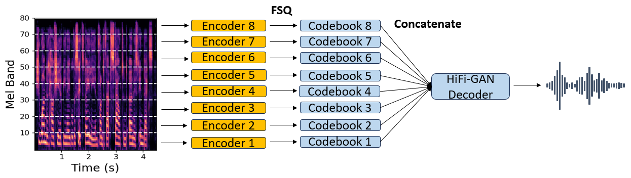
Fig. 1: Architecture of the proposed multi-band spectral codec. Disjoint mel-bands are encoded separately and quantized using an FSQ. All codebook embeddings are concatenated and given as input to a HiFi-GAN decoder which predicts the final waveform.

1 Introduction

Neural text-to-speech (TTS) systems typically consist of two neural models; an acoustic model which takes text as input and predicts a speech representation such as the mel-spectrogram, and a vocoder which takes the speech representation as input and predicts the audio waveform. Common acoustic models include Tacotron 2 [1], FastPitch [2], and FastSpeech 2 [3]. Common vocoders include HiFi-GAN [4], BigVGAN [5], and UnivNet [6].

Such systems have historically struggled with over-smoothness, which is a common problem that arises when teaching a model to predict continuous features with regression losses [7]. Using regression based reconstruction losses, such as L1- or L2-norm loss, results in predictions that are close to the ground truth but which are unrealistic, often looking too smooth or blurry. A common strategy to address this is to encode features into a latent space that can be predicted using a probabilistic loss function, often done using a variational autoencoder (VAE) as in VITS [8] or normalizing flows as in RadTTS [9].

Quantization is gaining popularity as an alternative means to feature encoding. Unlike VAEs and normalizing flows, quantization places no prior assumptions on the distribution of the latent space, enabling it to scale well to large datasets. Using discrete features also enables the use of powerful auto-regressive models, such as large language models, for speech synthesis. As a result neural audio codec models, which encode audio into a discrete latent space, are gaining visibility and often being used as an alternative to standard vocoders in speech synthesis systems. Some prominent neural audio codecs include EnCodec [10], SoundStream [11], AudioDec [12], and Descript Audio Codec [13]. Audio codecs such as these typically use an encoder-decoder network to encode the audio waveform, quantize it using a residual vector quantizer (RVQ), and decode the quantized features to reconstruct the original audio signal.

It has been shown that large language models, such as VALL-E [14] and SoundStorm [15], are able of synthesize audio with good quality when predicting audio codec tokens. However compared to previous speech synthesis models, these new models are very large, known to hallucinate, require reference audio, rely on large datasets that are difficult to collect at high sampling rates, and are either autoregressive or require complex and slow prediction functions such as iterative decoding. These factors make it challenging to utilize such models for real world applications.

In this paper we use the term non-autoregressive to refer to parallel models that predict all output tokens in a single iteration. We demonstrate that non-autoregressive TTS models generate low quality audio when trained with audio codecs. We describe a system for training a spectral codec which quantizes mel-spectrogram features into a simple flat codebook structure using a finite scalar quantizer (FSQ) [16]. The reconstructed audio from this spectral codec has perceptual quality comparable to audio codecs when evaluated on speech, while creating a discrete latent space that is easier for speech synthesis models to predict. We show that with a spectral codec, non-autoregressive TTS models can synthesize high-quality high-resolution audio. Audio samples highlighting our results are available online. All code for training our codec models is available open source [17]. We publicly release spectral codec models for 22.05kHz and 44.1kHz sampling rates, with 6.9 kbps bitrate.

2 Methodology

For this study we first compare the reconstruction quality of two audio codecs, three spectral codecs, and a HiFi-GAN baseline. We then evaluate the audio quality of FastPitch trained with each of these six models. In this section we summarize the architecture and training objective for each model.

2.1 Spectral Codec Architecture

To train our spectral codecs we use a modified version of the HiFi-GAN architecture [4]. HiFi-GAN is state of the art for mel-spectrogram inversion, and BigVGAN [5] showed that scaling HiFi-GAN results in a robust model that generalizes well to unseen speakers and non-speech data. AudioDec [12] showed that using an asymmetric network with a HiFi-GAN decoder can improve codec quality and latency.

For 44.1kHz audio we compute an 80-dimensional mel-spectrogram with a window size of 2048 samples and hop length of 512 samples. The spectrogram is passed through an encoder consisting of 6 HiFi-GAN V1 residual blocks, each with a hidden dimension of 256 and 1024 residual channels. We quantize the encoder output and then pass the discrete spectrogram features into a HiFi-GAN V1 decoder with upsample rates $[8,8,4,2]$ and 1024 initial channels to predict the audio waveform. The total size of this model is 65M parameters, with 10M in the encoder and 55M in the decoder.

We experiment with three different methods for quantizing the encoder output. First we use the RVQ setup from EnCodec [10] with eight codebooks, 1024 codes per codebook, and 128 codebook dimension. Second we use an FSQ with eight codebooks and codebook levels $[8,5,5,5]$, resulting in 1000 codes per codebook, and four dimensions per code, as suggested in [16]. This results in the original continuous 80-dimensional mel-spectrogram being compressed down to 32 quantized dimensions.

With the FSQ each output dimension is independent of each other, so the decision of how to group them into codebooks for audio token prediction is arbitrary. To address this we use a third multi-band quantization setup in which we create separate encoders for different groups of mel-bands. Since humans perceive mel-spectrogram bands as equally spaced, it makes sense to encode an equal number of bands into each codebook. To create the first codebook the first encoder quantizes mel-bands 0 through 10, the second encoder quantizes mel-bands 11 through 20 to create the second codebook, and so forth to create 8 codebooks from 80 mel-bands. A visualization of this is provided in Figure 1. To keep the total encoder size the same, each of the 8 multi-band encoders uses residual blocks with 128 hidden dimension and 256 residual channels.

Table 1: Speech reconstruction quality for signals reconstructed using codecs with different input features and quantizers.

Input Feature	Quantizer	MOS (Squim) $\uparrow$	ViSQOL $\uparrow$	Mel Distance $\downarrow$	STFT Distance $\downarrow$	SI-SDR (Squim) $\uparrow$	SI-SDR $\uparrow$
audio waveform	RVQ	$\textbf{4.40}~{}\bm{\pm}~{}\textbf{0.01}$	4.29 $\pm~{}0.01$	0.115 $\pm~{}0.001$	0.034 $\pm~{}0.000$	21.65 $\pm~{}0.20$	$\textbf{7.87}~{}\bm{\pm}~{}\textbf{0.14}$
audio waveform	FSQ	$\textbf{4.40}~{}\bm{\pm}~{}\textbf{0.01}$	4.28 $\pm~{}0.01$	0.114 $\pm~{}0.001$	0.034 $\pm~{}0.000$	$\textbf{21.72}~{}\bm{\pm}~{}\textbf{0.20}$	7.76 $\pm~{}0.14$
mel-spectrogram	–	4.37 $\pm~{}0.01$	$\textbf{4.70}~{}\bm{\pm}~{}\textbf{0.00}$	$\textbf{0.071}~{}\bm{\pm}~{}\textbf{0.001}$	$\textbf{0.031}~{}\bm{\pm}~{}\textbf{0.000}$	18.32 $\pm~{}0.19$	-23.08 $\pm~{}0.35$
mel-spectrogram	RVQ	4.36 $\pm~{}0.01$	$\textbf{4.42}~{}\bm{\pm}~{}\textbf{0.01}$	$\textbf{0.102}~{}\bm{\pm}~{}\textbf{0.001}$	0.034 $\pm~{}0.000$	19.02 $\pm~{}0.19$	-23.62 $\pm~{}0.32$
mel-spectrogram	FSQ	4.37 $\pm~{}0.01$	4.39 $\pm~{}0.01$	0.109 $\pm~{}0.001$	0.035 $\pm~{}0.000$	19.45 $\pm~{}0.19$	-22.85 $\pm~{}0.33$
multi-band mel	FSQ	4.37 $\pm~{}0.01$	4.40 $\pm~{}0.01$	$\textbf{0.103}~{}\bm{\pm}~{}\textbf{0.001}$	0.035 $\pm~{}0.000$	19.23 $\pm~{}0.17$	-21.92 $\pm~{}0.35$

Table 2: Speech synthesis quality for TTS models trained with different codecs.

Input Feature	Quantizer	Token Accuracy / % $\uparrow$	MOS (Squim) $\uparrow$	ViSQOL $\uparrow$	ESTOI $\uparrow$	SI-SDR (Squim) $\uparrow$
audio waveform	RVQ	6.67 $\pm~{}0.32$	3.98 $\pm~{}0.07$	3.14 $\pm~{}0.03$	0.60 $\pm~{}0.01$	15.08 $\pm~{}0.46$
audio waveform	FSQ	5.09 $\pm~{}0.30$	4.23 $\pm~{}0.06$	3.07 $\pm~{}0.02$	0.56 $\pm~{}0.01$	11.41 $\pm~{}0.49$
mel-spectrogram	–	–	4.23 $\pm~{}0.05$	3.86 $\pm~{}0.03$	0.74 $\pm~{}0.01$	18.68 $\pm~{}0.48$
mel-spectrogram	RVQ	10.93 $\pm~{}0.36$	4.31 $\pm~{}0.04$	3.57 $\pm~{}0.03$	0.69$\pm~{}0.01$	20.68 $\pm~{}0.42$
mel-spectrogram	FSQ	9.43 $\pm~{}0.35$	$\textbf{4.49}~{}\bm{\pm}~{}\textbf{0.03}$	$\textbf{3.84}~{}\bm{\pm}~{}\textbf{0.03}$	$\textbf{0.77}~{}\bm{\pm}~{}\textbf{0.01}$	21.65 $\pm~{}0.45$
multi-band mel	FSQ	$\textbf{12.61}~{}\bm{\pm}~{}\textbf{0.44}$	4.48 $\pm~{}0.03$	3.79 $\pm~{}0.03$	0.74 $\pm~{}0.01$	$\textbf{21.83}~{}\bm{\pm}~{}\textbf{0.38}$

Table 3: ASR performance on synthesized TTS audio.

Input Feature	Quantizer	WER / % $\downarrow$	CER / % $\downarrow$
ground truth	–	2.25 $\pm~{}0.48$	0.44 $\pm~{}0.09$
audio waveform	RVQ	3.13 $\pm~{}0.62$	1.01 $\pm~{}0.23$
audio waveform	FSQ	2.56  $\pm~{}0.53$	0.68 $\pm~{}0.15$
mel-spectrogram	–	2.52 $\pm~{}0.52$	0.68 $\pm~{}0.18$
mel-spectrogram	RVQ	2.36 $\pm~{}0.49$	0.55 $\pm~{}0.10$
mel-spectrogram	FSQ	2.30 $\pm~{}0.47$	0.50 $\pm~{}0.10$
multi-band mel	FSQ	2.31 $\pm~{}0.49$	0.50 $\pm~{}0.10$

2.2 Audio Codec Architecture

For our audio codecs we invert the HiFi-GAN decoder to create a symmetric encoder-decoder system. The encoder and decoder use symmetric downsampling and upsampling rates of $[2,4,8,8]$ and $[8,8,4,2]$ respectively. The encoder has 48 initial channels doubled after each down sample layer, and the decoder has 768 initial channels cut in half after each up sample layer. The total model size is 62M parameters. We train one version of the audio codec with an RVQ and one with an FSQ using the same parameters as the spectral codec. With these parameters, the audio and spectral codecs are similar in size and have equal token rates of 86.1 tokens per second and equal bitrates of 6.9 kbps.

2.3 Codec Training Objective

For reconstruction loss we use the multi-resolution mel-spectrogram loss introduced in [10] and the multi-resolution log-magnitude short-time Fourier transform (STFT) loss introduced in [6] with window lengths [32, 64, 128, 256, 512, 1024, 2048] with 25% hop length. As in [13] we use dimensions [5, 10, 20, 40, 80, 160, 320] for the mel-spectrogram loss. We use the multi-period discriminator introduced in [4] and the multi-scale complex STFT discriminator introduced in [10] both with squared-GAN and feature matching loss. The period discriminator is particularly important to include in the spectral codec training to improve its ability to estimate phase. As in [10] we update the discriminators only once every two steps.

All losses have a weight of 1.0, except the STFT loss which has a weight of 20.0. We observed that if the reconstruction losses were too small relative to the discriminator losses then the training was unstable as it would ignore the reconstruction task entirely after the discriminators were trained long enough.

2.4 TTS Architecture

For our TTS architecture we use a modified version of FastPitch [2]. FastPitch is a non-autoregressive transformer-based encoder-decoder system which takes text, pitch, and duration as input and predicts a mel-spectrogram. To improve quality we also condition the model on energy as in [3] and extract duration information during training using the alignment strategy in [18]. We normalize pitch and energy using speaker level mean and standard deviation.

The encoder and decoder both have six transformer layers with 512 latent dimension and 2048 convolutional filters. The encoder has eight attention heads while the decoder has a single attention head. The total model size is 88M parameters.

To predict audio tokens, we replace the L2 loss when predicting the mel-spectrogram with a softmax loss. As there are eight codebooks, we have eight softmax losses which predict the entries of the different codebooks in parallel. For the softmax we include logit normalization [19] with a temperature $\tau=0.02$.

Fig. 2: Mel-spectrogram examples: (a) ground truth speech, (b) TTS output generated from the audio codec with RVQ, and (c) TTS output generated from the multi-band spectral codec.

3 Experiments

3.1 Datasets

While most speech domains use 16 kHz audio, training high quality TTS models typically requires 22.05 kHz or ideally 44.1 kHz data. For TTS training we use HiFi-TTS [20], containing 300 hours of high quality 44.1 kHz audio from 10 speakers.

To train a robust audio codec we need a larger dataset. However most public datasets that are uploaded at 44.1 kHz contain upsampled mixed-bandwidth data. When audio codecs are trained on mixed bandwidth data, their quality degrades significantly as they fail to reconstruct frequencies above some bandwidth [21] which [13] suggests is the average bandwidth seen at training time.

To circumvent this, we create a large-scale 44.1 kHz dataset containing only full-bandwidth data. We take the metadata from the English subset of MLS [22] and download the original 48 kHz audiobooks from the Librivox website. We downsample to 44.1 kHz and use the bandwidth estimation strategy described in HiFi-TTS [20] to filter out all data with an estimated bandwidth below 16 kHz. In this way we create a new dataset containing 12.8k hours of full-bandwidth 44.1 kHz speech with 3.1M utterances and 2,776 speakers. We use this dataset for training our audio codecs. For evaluation we use the same test set as MLS with approximately 3.8k utterances from 42 speakers not seen in the training data.

3.2 Training

All codec models were trained for 100k training steps with a batch size of 16 examples per GPU and 16,384 audio samples ($\approx{0.37}$ seconds) per example, using an Adam optimizer with learning rate $2\cdot 10^{-4}$, $\beta_{1}=0.8$, $\beta_{2}=0.99$, and exponential learning rate decay with $\gamma=0.998$ per 1,000 steps.

All FastPitch models were trained for 1M training steps with a batch size of 8 per GPU, using an AdamW optimizer with learning rate $5\cdot 10^{-3}$, weight decay $10^{-6}$, $\beta_{1}=0.9$, $\beta_{2}=0.999$, and a Noam learning rate schedule with 1,000 warmup step.

All models were trained on eight V100 GPUs using NVIDIA NeMo [17].

3.3 Evaluation Method

For this study we evaluate the reconstruction performance of the codec models, and the performance of TTS models when trained on the corresponding audio tokens. Our baseline codec is an audio codec trained with an RVQ, similar to EnCodec. Our baseline TTS system is FastPitch with HiFi-GAN.

To evaluate performance we use a combination of instrumental metrics and informal listening tests. To evaluate perceptual quality we use ViSQOL [23] and estimate MOS with Torchaudio-Squim [24] using the ground truth audio signal as a reference. For measuring time-domain accuracy we use SI-SDR [25]. For measuring spectral accuracy we look at the L1 distance between log mel-spectrogram and log magnitude STFT features using window length 2048 and hop length 512. To measure intelligibility of TTS outputs we look at ESTOI [26] as well as the word error rate (WER) and character error rate (CER) of transcriptions using NVIDIA’s Fast Conformer-Transducer XL [27]. For reference we also include the test accuracy of the TTS models when predicting codec tokens. All metrics are reported with a $95\%$ confidence interval. For WER and CER we compute the confidence intervals with bootstrapping [28].

The difference in TTS performance between codecs is significant enough that we forgo a formal listening study and instead rely on estimated MOS and provide audio samples demonstrating the qualitative differences in the synthesized speech.

4 Results

4.1 Codec Performance

We first conduct an ablation study on the reconstruction quality of the codec models, with the results in Table 1. For reference we include a mel decoder with no quantization which is equivalent to HiFi-GAN. This provides an upper bound on the performance our spectral codec could achieve as we increase codebook size. HiFi-GAN performs significantly better in ViSQOL and mel-spectrogram reconstruction, but otherwise has comparable performance to codec models on other metrics. This suggests that the information loss from quantization has a relatively small effect on overall audio quality.

The instrumental metrics suggest that the reconstruction quality between all of the codecs are comparable, with the spectral codecs performing mildly better on mel-spectrogram reconstruction and ViSQOL, and the audio codecs performing better on waveform-based losses like SI-SDR.

Interestingly we see that our spectral codecs have very poor SI-SDR. This is because spectral codecs learn how to estimate realistic phase through adversarial training instead of directly encoding and decoding it from the waveform, causing the waveforms to be slightly misaligned. As a result standard time-domain losses, which assume the waveforms are temporally aligned, do not reflect the quality of the reconstructed signal. When we use Squim to estimate SDR without a reference audio there is much less degradation, which is more in line with the perceived quality.

We see no significant difference in reconstruction quality between the RVQ and FSQ with equal bitrate. This suggests that the hierarchical structure of the RVQ is not helping the compression algorithm while unnecessarily increasing the complexity of the prediction task for speech synthesis.

We observe similar trends during informal listening tests. For most utterances tested it is difficult for human listeners to perceive a significant difference between the codec reconstructions. This still holds true even for samples from Mozilla Common Voice [29] which contains out-of-domain speakers and languages not seen in the training data.

4.2 TTS Performance

We train our modified FastPitch architecture to predict the tokens of the five codec models, and the mel-spectrogram of the HiFi-GAN baseline. The results in terms on quality metrics are in Table 2 and the results in terms of ASR performance are in Table 3. We see a clear trend in which all automated metrics improve significantly when encoding the mel-spectrogram compared to the waveform, and when using FSQ compared to RVQ.

The relationship between token accuracy and perceived quality is less clear. Token accuracy increases when encoding the mel-spectrogram, decreases when using an FSQ with random codebook groups, and increases with the multi-band setup where the FSQ has well-defined codebook groups. Token accuracy is highest with the multi-band spectral codec, but otherwise produces similar quality audio to the full-band encoder.

Informal listening tests reveal some clear qualitative trends in the synthesized audio. All of our TTS models have poor audio quality when predicting audio codec tokens, even compared to other speech synthesis models, such as VALL-E [14]. We speculate that the performance difference is because we are using a non-autoregressive model and because our TTS system does not use a prompt from which it can copy over important information such as phase and acoustic conditions. Other studies with large auto-regressive language models have shown similar improvements in audio quality when using a spectral codec [30].

The baseline system with FastPitch and HiFi-GAN produces relatively noisy audio due to over-smoothness in the predicted mel-spectrogram. The system trained on the spectral codec with an RVQ sounds clear for the most part, but the audio tends to have noticeable differences in characteristics such as pitch, volume, and acoustics. This is consistent with other works, such as [15], which observe that with an RVQ most of the audio content is embedded in the early codebooks, with later codebooks containing more fine-grained acoustic details that need a more complex prediction method. Only the systems trained on spectral codecs with an FSQ produce high quality audio that is accurate to the ground truth.

5 Conclusion

In this work we proposed a system for training a spectral codec which quantizes mel-spectrogram features, as opposed to a typical codecs which work directly on time-domain audio signals. We performed an ablation study comparing the reconstruction quality of neural audio codec models with different input features and quantization methods. We found that all codecs with similar bitrate have comparable perceptual quality when evaluated with instrumental metrics on the task of speech reconstruction. This implies that quantizing mel-spectrograms, as opposed to time-domain signals, is not limiting the quality of the reconstructed signal. Furthermore, we trained non-autoregressive TTS models using audio tokens from the considered codecs and compared the quality of the generated speech signals. On the one hand, we observed that TTS models trained using time-domain codecs generate low-quality audio. On the other hand, TTS models trained using mel-spectrogram codecs generate audio with a significantly higher quality. We also found that TTS models perform better when predicting a flat codebook structure produced by FSQ, compared to a hierarchical codebook structure produced by the widely used RVQ. We have observed similar performance trends with other speech synthesis systems, which we intend to expand on in future works.

References

- [1] Jonathan Shen, Ruoming Pang, Ron J Weiss, Mike Schuster, Navdeep Jaitly, Zongheng Yang, Zhifeng Chen, Yu Zhang, Yuxuan Wang, Rj Skerrv-Ryan, et al., “Natural TTS synthesis by conditioning wavenet on mel spectrogram predictions,” in Proc. IEEE Int. Conf. on Acoustics, Speech and Signal Process. (ICASSP), 2018, pp. 4779–4783.
- [2] Adrian Łańcucki, “FastPitch: Parallel text-to-speech with pitch prediction,” in Proc. IEEE Int. Conf. on Acoustics, Speech and Signal Process. (ICASSP), pp. 6588–6592. 2021.
- [3] Yi Ren, Chenxu Hu, Xu Tan, Tao Qin, Sheng Zhao, Zhou Zhao, and Tie-Yan Liu, “FastSpeech 2: Fast and high-quality end-to-end text to speech,” in Proc. International Conference on Learning Representations (ICLR). 2021.
- [4] Jungil Kong, Jaehyeon Kim, and Jaekyoung Bae, “HiFi-GAN: Generative adversarial networks for efficient and high fidelity speech synthesis,” in Proc. Conf. on Neural Information Process. Systems (NeurIPS). 2020.
- [5] Sang gil Lee, Wei Ping, Boris Ginsburg, Bryan Catanzaro, and Sungroh Yoon, “BigVGAN: A universal neural vocoder with large-scale training,” in Proc. International Conference on Learning Representations (ICLR). 2023.
- [6] Won Jang, Dan Lim, Jaesam Yoon, Bongwan Kim, and Juntae Kim, “UnivNet: A neural vocoder with multi-resolution spectrogram discriminators for high-fidelity waveform generation,” arXiv preprint arXiv:2106.07889, 2021.
- [7] Yi Ren, Xu Tan, Tao Qin, Zhou Zhao, and Tie-Yan Liu, “Revisiting over-smoothness in text to speech,” in Proc. 60th Annual Meeting of the Association for Computational Linguistics, 2022.
- [8] Jaehyeon Kim, Jungil Kong, and Juhee Son, “Conditional variational autoencoder with adversarial learning for end-to-end text-to-speech,” in Proc. International Conference on Machine Learning (ICML). 2021.
- [9] Kevin J. Shih, Rafael Valle, Rohan Badlani, Adrian Lancucki, Wei Ping, and Bryan Catanzaro, “RAD-TTS: Parallel flow-based TTS with robust alignment learning and diverse synthesis,” in Proc. ICML Workshop on Invertible Neural Networks, Normalizing Flows, and Explicit Likelihood Models, 2021.
- [10] Alexandre Défossez, Jade Copet, Gabriel Synnaeve, and Yossi Adi, “High fidelity neural audio compression,” arXiv preprint arXiv:2210.13438, 2022.
- [11] Neil Zeghidour, Alejandro Luebs, Ahmed Omran, Jan Skoglund, and Marco Tagliasacchi, “Soundstream: An end-to-end neural audio codec,” IEEE/ACM Transactions on Audio, Speech, and Language Processing, vol. 30, pp. 495–507, 2021.
- [12] Yi-Chiao Wu, Israel D Gebru, Dejan Marković, and Alexander Richard, “AudioDec: An open-source streaming high-fidelity neural audio codec,” in Proc. IEEE Int. Conf. on Acoustics, Speech and Signal Process. (ICASSP), 2023.
- [13] Rithesh Kumar, Prem Seetharaman, Alejandro Luebs, Ishaan Kumar, and Kundan Kumar, “High-fidelity audio compression with improved RVQGAN,” in Proc. Conf. on Neural Information Process. Systems (NeurIPS), 2023.
- [14] Chengyi Wang, Sanyuan Chen, Yu Wu, Ziqiang Zhang, Long Zhou, Shujie Liu, Zhuo Chen, Yanqing Liu, Huaming Wang, Jinyu Li, Lei He, Sheng Zhao, and Furu Wei, “Neural codec language models are zero-shot text to speech synthesizers,” arXiv preprint arXiv:2301.02111, 2023.
- [15] Zalán Borsos, Matt Sharifi, Damien Vincent, Eugene Kharitonov, Neil Zeghidour, and Marco Tagliasacchi, “SoundStorm: Efficient parallel audio generation,” arXiv preprint arXiv:2305.09636, 2023.
- [16] Fabian Mentzer, David Minnen, Eirikur Agustsson, and Michael Tschannen, “Finite scalar quantization: VQ-VAE made simple,” in Proc. International Conference on Learning Representations (ICLR). 2024.
- [17] Eric Harper, Somshubra Majumdar, Oleksii Kuchaiev, Li Jason, Yang Zhang, Evelina Bakhturina, Vahid Noroozi, Sandeep Subramanian, Koluguri Nithin, Huang Jocelyn, Fei Jia, Jagadeesh Balam, Xuesong Yang, Micha Livne, Yi Dong, Sean Naren, and Boris Ginsburg, “Nemo: a toolkit for conversational ai and large language models,” .
- [18] Rohan Badlani, Adrian Łancucki, Kevin J. Shih, Rafael Valle, Wei Ping, and Bryan Catanzaro, “One TTS alignment to rule them all,” in Proc. IEEE Int. Conf. on Acoustics, Speech and Signal Process. (ICASSP). 2021.
- [19] Hongxin Wei, Renchunzi Xie, Hao Cheng, Lei Feng, Bo An, and Yixuan Li, “Mitigating neural network overconfidence with logit normalization,” in Proc. International Conference on Machine Learning (ICML). 2022.
- [20] Evelina Bakhturina, Vitaly Lavrukhin, Boris Ginsburg, and Yang Zhang, “Hi-Fi multi-speaker English TTS dataset,” arXiv preprint arXiv:2104.01497, 2021.
- [21] Krishna C. Puvvada, Nithin Rao Koluguri, Kunal Dhawan, Jagadeesh Balam, and Boris Ginsburg, “Discrete audio representation as an alternative to mel-spectrograms for speaker and speech recognition,” in Proc. IEEE Int. Conf. on Acoustics, Speech and Signal Proc. (ICASSP), 2024.
- [22] Vineel Pratap, Qiantong Xu, Anuroop Sriram, Gabriel Synnaeve, and Ronan Collobert, “MLS: A large-scale multilingual dataset for speech research,” in Proc. Interspeech. Oct. 2020, ISCA.
- [23] Andrew Hines, Jan Skoglund, Anil C Kokaram, and Naomi Harte, “ViSQOL: an objective speech quality model,” EURASIP Journal on Audio, Speech, and Music Processing, vol. 2015, no. 1, pp. 1–18, 2015.
- [24] Anurag Kumar, Ke Tan, Zhaoheng Ni, Pranay Manocha, Xiaohui Zhang, Ethan Henderson, and Buye Xu, “TorchAudio-Squim: Reference-less speech quality and intelligibility measures in torchaudio,” in Proc. IEEE Int. Conf. on Acoustics, Speech and Signal Process. (ICASSP). 2023.
- [25] Jonathan Le Roux, Scott Wisdom, Hakan Erdogan, and John R. Hershey, “SDR - half-baked or well done?,” in Proc. IEEE Int. Conf. on Acoustics, Speech and Signal Process. (ICASSP). 2019.
- [26] Jesper Jensen and Cees H. Taal, “An algorithm for predicting the intelligibility of speech masked by modulated noise maskers,” IEEE/ACM Transactions on Audio, Speech, and Language Processing, vol. 24, no. 11, pp. 2009–2022, 2016.
- [27] NVIDIA, “STT En Fast Conformer-Transducer XLarge,” https://catalog.ngc.nvidia.com/orgs/nvidia/teams/nemo/models/stt_en_fastconformer_transducer_xlarge, 2023, [Online; accessed Feb-2024].
- [28] M. Bisani and H. Ney, “Bootstrap estimates for confidence intervals in ASR performance evaluation,” in Proc. IEEE Int. Conf. on Acoustics, Speech and Signal Process. (ICASSP), 2004, vol. 1, pp. I–409.
- [29] Rosana Ardila, Megan Branson, Kelly Davis, Michael Henretty, Michael Kohler, Josh Meyer, Reuben Morais, Lindsay Saunders, Francis M. Tyers, and Gregor Weber, “Common Voice: A massively-multilingual speech corpus,” in Proc. Conf. on Language Resources and Evaluation (LREC). 2020.
- [30] Paarth Neekhara, Shehzeen Hussain, Subhankar Ghosh, Jason Li, Rafael Valle, Rohan Badlani, and Boris Ginsburg, “Improving robustness of LLM-based speech synthesis by learning monotonic alignment,” Proc. Interspeech, 2024, to appear.