Markov chain Monte Carlo without evaluating the target: an auxiliary variable approach

Abstract

In sampling tasks, it is common for target distributions to be known up to a normalising constant. However, in many situations, evaluating even the unnormalised distribution can be costly or infeasible. This issue arises in scenarios such as sampling from the Bayesian posterior for tall datasets and the ‘doubly-intractable’ distributions. In this paper, we begin by observing that seemingly different Markov chain Monte Carlo (MCMC) algorithms, such as the exchange algorithm (Murray et al.,, 2006), PoissonMH (Zhang and De Sa,, 2019), and TunaMH (Zhang et al.,, 2020), can be unified under a simple common procedure. We then extend this procedure into a novel framework that allows the use of auxiliary variables in both the proposal and acceptance–rejection steps. We develop the theory of the new framework, applying it to existing algorithms to simplify and extend their results. Several new algorithms emerge from this framework, with improved performance demonstrated on both synthetic and real datasets.

Keywords: Markov chain Monte Carlo, auxiliary variable, tall dataset, exchange algorithm, locally–balanced proposal, stochastic gradient Langevin dynamics

1 Introduction

The general workflow of Markov chain Monte Carlo algorithms is similar, yet computational challenges arise in their own way. Interestingly, solutions to these unique challenges sometimes also share a common underlying principle, which often go unnoticed even by their proposers. This paper aims to explore this phenomenon by providing a unified framework for various MCMC algorithms across Bayesian inference applications. New algorithms also emerge from this framework.

We briefly recall the workflow of Metropolis–Hastings type algorithms (Metropolis et al.,, 1953; Hastings,, 1970), one of the most general and popular MCMC methods. Given a target distribution, these methods typically iterate over a two-step process: they first propose a new state from a proposal distribution, given the current state. Then, they apply an acceptance–rejection mechanism to decide if the transition to the new state should occur. While the choices of the proposal vary by algorithm, their implementation often requires evaluating the unnormalised distribution—that is, the target distribution up to a scaling factor. Several algorithms such as the Metropolis–adjusted Langevin algorithm (MALA) (Besag,, 1994) and Hamiltonian Monte Carlo (HMC) (Duane et al.,, 1987) also require evaluating the derivative of the unnormalised distribution.

In Bayesian inference, users focus on quantities associated with the posterior distribution $\pi(\theta\mid x)$, with $x$ as observed data and $\theta$ as the parameter of interest. Given a prior $\pi(\theta)$ and likelihood $p_{\theta}(x)$, the posterior distribution is $\pi(\theta\mid x)=\pi(\theta)p_{\theta}(x)/\int p_{\theta}(x)\pi(\mathrm{d}\theta)$. To ‘understand’ the typically complex posterior, MCMC is often the go-to strategy. Establishing a prior, selecting an MCMC algorithm aimed at the posterior, and examining posterior samples constitute the process of the modern Bayesian inference, with MCMC acting as the backbone. For a detailed historical background, see Martin et al., (2024).

Although MCMC needs only the unnormalised posterior, which is $\pi(\theta)p_{\theta}(x)$ as a function of $\theta$ for fixed $x$, challenges still arise when evaluating this function is expensive or not feasible. The difficulty can stem from both the $\theta$ and the $x$ side. Consider the following scenarios:

Scenario 1 (Expensive $\theta$: Doubly-intractable distribution).

Suppose the model likelihood $p_{\theta}(x)$ is expressed as $f_{\theta}(x)/Z(\theta)$, with $Z(\theta)$ requiring a high-dimensional integration or the summation of an exponential number of terms, making it costly or impossible to compute directly. Standard Metropolis–Hastings type algorithms cannot be directly applied to these problems, as they necessitate calculating the ratio $Z(\theta^{\prime})/Z(\theta)$ at each step in its acceptance–rejection process. The posterior distribution $\pi(\theta\mid x)\propto\pi(\theta)f_{\theta}(x)/Z(\theta)$ is called the “doubly-intractable distribution”, a term coined by Murray et al., (2006). This distribution has found use in large graphical models (Robins et al.,, 2007; Besag,, 1986), autologistic models for spatial data (Besag,, 1974), permutation models (Vitelli et al.,, 2018; Diaconis and Wang,, 2018), spatial point processes (Strauss,, 1975), matrix-valued data (Hoff,, 2009; Rao et al.,, 2016), among many others.

Scenario 2 (Expensive $x$: Tall Dataset).

Imagine that users have gathered a large dataset $x=(x_{1},\ldots,x_{N})$, where $N$ can be in the millions or billions. Each data point is independently and identically distributed following the distribution $\mathsf{p}_{\theta}$. In this case, the joint model likelihood is $p_{\theta}(x)=\prod_{i=1}^{N}\mathsf{p}_{\theta}(x_{i})$. However, executing standard Metropolis–Hastings algorithms becomes expensive, as the per-step acceptance–rejection computation requires evaluations across the full dataset. This scenario is often referred to as “tall data” (Bardenet et al.,, 2017), which represents the kind of datasets commonly found in machine learning tasks (Welling and Teh,, 2011; Ahn,, 2015).

Various approaches have been proposed to address these challenges. Here, we review three algorithms: the exchange algorithm (Algorithm 1, Murray et al., (2006)) for doubly-intractable distributions; PoissonMH (Algorithm 2, Zhang and De Sa, (2019)) and TunaMH (Algorithm 3, Zhang et al., (2020)) for tall datasets. These algorithms have demonstrated promising empirical performance compared to other existing solutions, and are most relevant to our proposed framework and new algorithms. Additional relevant studies will be discussed in Section 1.2. For completeness, the beginning of each algorithm’s pseudocode contains a section titled “promise,” which describes the technical assumptions and practical prerequisites that users need to know before executing the algorithm. It is worth noting that the posterior with $N$ i.i.d. data points satisfies this promise of PoissonMH (and TunaMH) by setting $\phi_{i}(\theta,x):=N^{-1}\log\pi(\theta)+\log\mathsf{p}_{\theta}(x_{i})$ (and $U_{i}(\theta,x):=-N^{-1}\log\pi(\theta)-\log\mathsf{p}_{\theta}(x_{i}))$.)

Algorithm 1 Exchange Algorithm

1:  Promise:

• Target $\pi(\theta\mid x)\propto\pi(\theta)p_{\theta}(x)$,

• Likelihood $p_{\theta}(x)=f_{\theta}(x)/Z(\theta)$ where the value of $f_{\theta}$ can be queried

• A simulator ${\mathcal{S}}(\cdot)$ with input $\theta$. Each run outputs a random variable $w\sim p_{\theta}$

2:  Initialise: Initial state $\theta_{0}$, proposal $q$; number of iterations $T$

3:  for $t=0$ to $T-1$ do

4:     propose $\theta^{\prime}\sim q(\theta_{t},\cdot)$

5:     sample $\omega\sim{\mathcal{S}}(\cdot)$

6:     compute

$$r\xleftarrow{}\frac{\pi(\theta^{\prime})f_{\theta^{\prime}}(x)f_{\theta_{t}}(\omega)}{\pi(\theta_{t})f_{\theta_{t}}(x)f_{\theta^{\prime}}(\omega)}\cdot\frac{q(\theta^{\prime},\theta_{t})}{q(\theta_{t},\theta^{\prime})}$$

7:     with probability $\min\{1,r\}$, set $\theta_{t+1}\xleftarrow{}\theta^{\prime}$; otherwise, $\theta_{t+1}\xleftarrow{}\theta_{t}$

8:  end for

Algorithm 2 PoissonMH

1:  Promise:

• Target $\pi(\theta\mid x)\propto\exp{\{\sum_{i=1}^{N}\phi_{i}(\theta;x)\}}$,

• For every $\theta$, each $\phi_{i}(\theta;x)\in[0,M_{i}]$ with some $M_{i}>0$

2:  Initialise: Initial state $\theta_{0}$; proposal $q$; hyperparameter $\lambda$; set $L:=\sum_{i=1}^{N}M_{i}$; number of iterations $T$

3:  for $t=0$ to $T-1$ do

4:     propose $\theta^{\prime}\sim q(\theta_{t},\cdot)$

5:     sample $s_{i}\sim\mathsf{Poi}\left(\frac{\lambda M_{i}}{L}+\phi_{i}(\theta_{t};x)\right)$ for each $i\in\{1,2,\ldots,N\}$, form minibatch $S=\{i\mid s_{i}>0\}$

6:     compute

$$r\xleftarrow{}\frac{\exp\left\{\sum_{i\in S}s_{i}\log\left(1+\frac{L}{\lambda M_{i}}\phi_{i}(\theta^{\prime};x)\right)\right\}}{\exp\left\{\sum_{i\in S}s_{i}\log\left(1+\frac{L}{\lambda M_{i}}\phi_{i}(\theta_{t};x)\right)\right\}}\cdot\frac{q(\theta^{\prime},\theta_{t})}{q(\theta_{t},\theta^{\prime})}$$

7:     with probability $\min\{1,r\}$, set $\theta_{t+1}\xleftarrow{}\theta^{\prime}$; otherwise $\theta_{t+1}\xleftarrow{}\theta_{t}$

8:  end for

Algorithm 3 TunaMH

1:  Promise:

• Target $\pi(\theta\mid x)\propto\exp{\{-\sum_{i=1}^{N}U_{i}(\theta;x)\}}$,

• For every $\theta$ and $\theta^{\prime}$, each $|U_{i}(\theta^{\prime};x)-U_{i}(\theta;x)|\leq c_{i}M(\theta,\theta^{\prime})$ for some symmetric non-negative function $M$ and positive constants $c_{i}$

2:  Initialise: Initial state $\theta_{0}$; proposal $q$; hyperparameter $\chi$; set $C=\sum_{i=1}^{N}c_{i}$; number of iterations $T$

3:  for $t=0$ to $T-1$ do

4:     propose $\theta^{\prime}\sim q(\theta_{t},\cdot)$ and compute $M(\theta_{t},\theta^{\prime})$

5:     set $\lambda=\chi C^{2}M^{2}(\theta,\theta^{\prime})$

6:     sample $s_{i}\sim\mathsf{Poi}(\frac{\lambda c_{i}}{C}+\phi_{i}(\theta_{t},\theta^{\prime};x))$ where $\phi_{i}(\theta_{t},\theta^{\prime};x)=\frac{U_{i}(\theta^{\prime};x)-U_{i}(\theta_{t};x)}{2}+\frac{c_{i}}{2}M(\theta_{t},\theta^{\prime})$, for each $i\in\{1,2,\cdots,N\}$, form minibatch $S=\{i\mid s_{i}>0\}$

7:     compute

$$r\xleftarrow{}\frac{\exp\left\{\sum_{i\in S}s_{i}\log\left(1+\frac{C}{\lambda c_{i}}\phi_{i}(\theta^{\prime},\theta_{t};x)\right)\right\}}{\exp\left\{\sum_{i\in S}s_{i}\log\left(1+\frac{C}{\lambda c_{i}}\phi_{i}(\theta_{t},\theta^{\prime};x)\right)\right\}}\cdot\frac{q(\theta^{\prime},\theta_{t})}{q(\theta_{t},\theta^{\prime})}$$

8:     with probability $\min\{1,r\}$, set $\theta_{t+1}\xleftarrow{}\theta^{\prime}$; otherwise $\theta_{t+1}\xleftarrow{}\theta_{t}$

9:  end for

The similarities and differences among these algorithms are both clear. These algorithms share the goal of sampling from the posterior without directly computing the target distribution, preserving the correct stationary distribution. However, their methodologies differ. The exchange algorithm targets doubly-intractable distributions, assuming access to a simulator for synthetic data. PoissonMH and TunaMH address the ‘tall data’ problem by avoiding full dataset evaluations and impose different assumptions on the model likelihood. This prompts the question: Can these algorithms be unified under a common framework?

1.1 Our contribution

Our first contribution answers the above question affirmatively. We begin with a key observation: the exchange, PoissonMH, and TunaMH algorithms can be unified into a simple common procedure, detailed in Section 2. This procedure reveals their inherent similarities.

Furthermore, we take a step further to develop new algorithms. We notice that existing algorithms without evaluating the full posterior predominantly support random-walk-type proposals—which mix slowly in high-dimensional sampling problems. Motivated by this, our major contribution is a novel framework in Section 3.2. Thanks to this framework, we develop new gradient-based minibatch algorithms that allow users to choose a high-efficiency proposal. We develop new variants of ‘locally balanced proposals’ (Zanella,, 2020; Livingstone and Zanella,, 2022) and Stochastic Gradient Langevin Dynamics (SGLD) (Welling and Teh,, 2011) to improve the PoissonMH and TunaMH. These algorithms support gradient-based proposals while maintaining correct stationary distribution with minibatch data. They show significant efficiency improvements on synthetic and real datasets compared to their predecessors and standard algorithms like random-walk Metropolis, MALA, and HMC.

The framework itself may be of independent interest. Methodologically, it appears to be flexible and practical. It uses auxiliary variables in both the proposal and acceptance-rejection steps, encompassing previous frameworks Titsias and Papaspiliopoulos, (2018) and Section 2, which both focus on only one aspect. This offers greater potential for further algorithm design. Theoretically, the framework is linked to the theory of Markov chain comparison, an active area with recent progress (Andrieu et al.,, 2022; Power et al.,, 2024; Qin et al.,, 2023; Ascolani et al.,, 2024). Both classical (Diaconis and Saloff-Coste,, 1993; Dyer et al.,, 2006) and recent techniques are well-suited for analysing the framework or its applications. Our theoretical analysis in Section 4 can recover, strengthen, and extend several existing results in a simpler way.

1.2 Related works

Both the doubly-intractable problem (Scenario 1) and tall dataset problem (Scenario 2) are studied extensively in statistics and machine learning. Here we provide a concise review of the related literature. The exchange algorithm (Algorithm 1) is widely used for doubly-intractable problems, with extensions by Liang, (2010), Liang et al., (2016), and Alquier et al., (2016) improving its efficiency or relaxing its assumptions. Theoretical properties are examined in Nicholls et al., (2012) and Wang, (2022). It fits within a broader framework introduced in Andrieu et al., 2018b . Another popular solution by Møller et al., (2006) falls within the pseudo-marginal MCMC framework (Lin et al.,, 2000; Beaumont,, 2003; Andrieu and Roberts,, 2009). Their theory is studied in Andrieu and Roberts, (2009); Andrieu and Vihola, (2015). Other solutions include the ‘Russian-Roulette sampler’ (Lyne et al.,, 2015).

For tall datasets, many minibatch MCMC algorithms reduce iteration costs. These are classified into exact and inexact methods, based on whether they maintain the target distribution as stationary. Inexact methods, such as those in Welling and Teh, (2011); Chen et al., (2014); Korattikara et al., (2014); Quiroz et al., (2018); Dang et al., (2019); Wu et al., (2022), introduce a systematic bias to trade off for implementation efficiency. Zhang et al., (2020) demonstrate that this bias can accumulate significantly, even when the bias per-step is arbitrarily small. In contrast, exact methods such as Maclaurin and Adams, (2014); Bardenet et al., (2017); Cornish et al., (2019); Zhang and De Sa, (2019); Zhang et al., (2020) maintain the correct stationary distribution but rely on assumptions about the target distribution. This paper primarily focuses on Zhang et al., (2020) and its predecessor Zhang and De Sa, (2019), as they show improved empirical performance with relatively mild assumptions. Non-reversible exact methods by Bouchard-Côté et al., (2018); Bierkens et al., (2019) are also appealing but can be challenging to implement. In addition to minibatch MCMC algorithms, divide-and-conquer algorithms by Huang and Gelman, (2005); Wang and Dunson, (2013); Neiswanger et al., (2014) are suitable for parallel implementation.

1.3 Notations

Let $\Theta$ be a measurable space with $\sigma$-algebra ${\mathcal{F}}$. We preserve the letter $x$ to denote all the observed data and $\pi(\cdot\mid x)$ to denote the posterior distribution with prior $\pi(\theta)$ and likelihood $p_{\theta}(x)$. For probability distributions $P$ and $Q$, their total-variation (TV) distance is $d_{\sf TV}(P,Q):=\sup_{A}\lvert P(A)-Q(A)\rvert$, and Kullback–Leibler (KL) divergence is $d_{\sf KL}(P||Q):=\int\log\left((P/Q)(\mathrm{d}x)\right)P(\mathrm{d}x)$ given $P$ is absolutely continuous with respect to $Q$. Given a differentiable function $f(x,\theta)$ with $x\in\mathbb{R}^{m}$ and $\theta\in\mathbb{R}^{n}$, we define $\theta_{i}$ as $\partial_{\theta_{i}}f:=\partial f/\partial\theta_{i}$, and $\nabla_{\theta}f:=\left(\partial_{\theta_{1}}f,\partial_{\theta_{2}}f,\cdots,\partial_{\theta_{n}}f\right)$. Similarly, we define $\partial_{x_{j}}f,\nabla_{x}f$. We denote $\lVert x\rVert_{p}:=\left(\lvert x_{1}\rvert^{p}+\lvert x_{2}\rvert^{p}+\ldots\lvert x_{m}\rvert^{p}\right)^{1/p}$ for $p>0$. We use $\mathsf{Poi}(\cdot),\mathbb{N}(\cdot,\cdot),$ and $\mathsf{Unif}(\cdot,\cdot)$ to denote the Poisson, Gaussian, and uniform distribution, respectively. In particular, $\mathsf{Unif}(A,k)$ represents $k$ elements uniformly chosen from a finite set $A$ without replacement.

1.4 Organization

We present a common procedure that unifies the exchange algorithm, PoissonMH, and TunaMH in Section 2. Our main framework extends this further and is presented as a meta-algorithm (Algorithm 4) in Section 3. Section 3.3 introduces new algorithms as special cases of our meta-algorithm. Section 4 provides a theory for the mixing time of Algorithm 4, with applications in Section 4.4. Section 5 demonstrates the effectiveness of our new algorithms through three experiments. Section 6 concludes this paper with future directions. Additional proofs, experiment details, and extra experiments are provided in the supplementary.

2 A common procedure of existing algorithms

Although Algorithm 1, 2, and 3 differ significantly, they all follow the following procedure at each step. Given target distribution $\pi(\cdot\mid x)$, a proposal kernel $q(\cdot,\cdot)$, and current state $\theta$:

1. Propose a new state $\theta^{\prime}\sim q(\theta,\cdot)$

2. Generate an auxiliary variable $\omega$ according to certain distribution denoted as $P_{\theta\rightarrow\theta^{\prime}}(\cdot)$

3. Construct an estimator $R_{\theta\rightarrow\theta^{\prime}}(w)$ for $\pi(\theta^{\prime}\mid x)/\pi(\theta\mid x)$, set $r:=R_{\theta\rightarrow\theta^{\prime}}(w)q(\theta^{\prime},\theta)/q(\theta,\theta^{\prime})$

4. With probability $\min\{r,1\}$, set $\theta_{\mathsf{new}}:=\theta^{\prime}$. Otherwise, $\theta_{\mathsf{new}}:=\theta$.

Compared to standard Metropolis–Hastings algorithms, this method uses an estimator based on an auxiliary variable to estimate the target ratio $\pi(\theta^{\prime}\mid x)/\pi(\theta\mid x)$ instead of directly computing it. This procedure still defines a Markov chain on $\Theta$. It will also preserve $\pi(\cdot\mid x)$ as the stationary distribution if the following equation is satisfied:

Proposition 1.

Let $K$ be the one-step Markov transition kernel defined by the process described above. Suppose for every $\theta,\theta^{\prime}\in\Theta\times\Theta$, the estimator $R_{\theta\rightarrow\theta^{\prime}}(\omega)$ satisfies

$$R_{\theta\rightarrow\theta^{\prime}}(\omega)\pi(\theta\mid x)P_{\theta\rightarrow\theta^{\prime}}(\omega)=\pi(\theta^{\prime}\mid x)P_{\theta^{\prime}\rightarrow\theta}(\omega).$$ (1)

Then $R_{\theta\rightarrow\theta^{\prime}}$ is unbiased for $\pi(\theta^{\prime}\mid x)/\pi(\theta\mid x)$ and $K$ is reversible with respect to $\pi(\theta\mid x)$.

Now we can verify Algorithm 1, 2, and 3 all satisfy equation (1) in Proposition 1. Detailed calculations verifying the next three examples are provided in supplementary A.2.

Example 1 (Exchange algorithm).

Recall $\pi(\theta|x)\propto p(\theta)\frac{f_{\theta}(x)}{Z(\theta)}$ for doubly-intractable distributions. The auxiliary variable $\omega$ is an element in the sample space. Meanwhile:

• The distribution $P_{\theta\rightarrow\theta^{\prime}}(\omega):=p_{\theta^{\prime}}(\omega)=f_{\theta^{\prime}}(\omega)/Z(\theta^{\prime})$.

• The estimator

  $$R_{\theta\rightarrow\theta^{\prime}}(\omega):=\frac{\pi(\theta^{\prime})f_{\theta^{\prime}}(x)f_{\theta}(\omega)}{\pi(\theta)f_{\theta}(x)f_{\theta^{\prime}}(\omega)}.$$

Example 2 (PoissonMH).

PoissonMH (Algorithm 2) aims to sample from $\pi(\theta\mid x)\propto\exp(\sum_{i=1}^{N}\phi_{i}(\theta;x))$. The auxiliary variable $\omega=(s_{1},s_{2},\cdots,s_{N})$ belongs to $\{0,1,2,\cdots\}^{N}$, i.e., a vector of natural numbers with the same length as the number of data points. Each component of $\omega$ follows an independent Poisson distribution. More precisely:

• The distribution $P_{\theta\rightarrow\theta^{\prime}}:=\bigotimes_{i=1}^{N}\mathsf{Poi}\left(\frac{\lambda M_{i}}{L}+\phi_{i}(\theta;x)\right)$.

• The estimator

  $$R_{\theta\rightarrow\theta^{\prime}}(\omega):=\frac{\exp\left\{\sum_{i\in S}s_{i}\log\left(1+\frac{L}{\lambda M_{i}}\phi_{i}(\theta^{\prime};x)\right)\right\}}{\exp\left\{\sum_{i\in S}s_{i}\log\left(1+\frac{L}{\lambda M_{i}}\phi_{i}(\theta;x)\right)\right\}},$$

  with all the notations defined in Algorithm 2. The estimator relies solely on data points in $S$. By selecting appropriate parameters, the expected size of $S$ can be much smaller than $N$, thereby reducing the computational cost per iteration.

Example 3 (TunaMH).

TunaMH (Algorithm 3) aims to solve the same problem as PoissonMH under more practical assumptions. Similar to PoissonMH, the auxiliary variable $\omega=(s_{1},s_{2},\cdots,s_{N})\in\{0,1,2,\cdots\}^{N}$. Meanwhile:

• The distribution $P_{\theta\rightarrow\theta^{\prime}}:=\bigotimes_{i=1}^{N}\mathsf{Poi}\left(\frac{\lambda c_{i}}{C}+\phi_{i}(\theta,\theta^{\prime};x)\right)$.

• The estimator

  $$R_{\theta\rightarrow\theta^{\prime}}(\omega):=\frac{\exp\left\{\sum_{i\in S}s_{i}\log\left(1+\frac{C}{\lambda c_{i}}\phi_{i}(\theta^{\prime},\theta;x)\right)\right\}}{\exp\left\{\sum_{i\in S}s_{i}\log\left(1+\frac{C}{\lambda c_{i}}\phi_{i}(\theta,\theta^{\prime};x)\right)\right\}}.$$

  with all the notations defined in Algorithm 3.

We provide two remarks here. An additioanl comment is provided in supplementary C. First, the novelty of our finding in this section lies in discovering the inherent connections between algorithms designed for doubly-intractable distributions and those for tall datasets. The common procedure itself is not new. In Section 2.1 of Andrieu et al., 2018a , the authors present a slightly broader framework in which they substitute $P_{\theta^{\prime}\rightarrow\theta}(\omega)$ with $P_{\theta^{\prime}\rightarrow\theta}(\varphi(\omega))$, where $\varphi$ represents any measurable involution. Therefore our framework can be viewed as taking $\varphi=\mathsf{id}$, the identity map. On the other hand, the primary goal in Andrieu et al., 2018a is to improve the quality of the estimator within the exchange algorithm while preserving the stationary distribution. Consequently, they do not consider tall datasets.

Second, it is interesting to observe that Algorithm 1, 2, and 3 use three different ways of generating the auxiliary variable. In the exchange algorithm, $\omega$ depends on $\theta^{\prime}$; in PoissonMH, it depends on $\theta$; and in TunaMH, it depends on both. While this may appear as a simple finding, it will significantly impact the design of new algorithms in Section 3.

The current common procedure already provides a convenient basis for analysing the theory behind these algorithms. Nevertheless, we choose to postpone the theoretical analysis after Section 3, where a more comprehensive framework will be introduced. Analysing the general framework allows us to simplify and improve existing results as corollaries.

3 A new framework with (two) auxiliary variables

3.1 Motivation: gradient-based proposal design

The exchange algorithm, PoissonMH, and TunaMH predominantly involve either independent or random-walk proposals, which scale poorly with dimensionality. Gradient-based MCMC algorithms, like MALA and HMC, are considered much more efficient.

One simple idea is to choose $q$ as a gradient-based proposal in Section 2. However, upon second thought, one will quickly realise the challenges in implementing such a strategy: For the doubly-intractable distribution, the gradient of log-posterior involves the intractable $\nabla_{\theta}\log(Z(\theta))$. For tall datasets, computing the gradient requires evaluating the entire dataset, conflicting with the goal of reducing iteration costs in minibatch MCMC algorithms like PoissonMH and TunaMH.

Nevertheless, designing an ‘informed proposal’ remains a fascinating idea. Motivated by this, we introduce a novel framework in Section 3.2, extending Section 2. This framework leads to new algorithms using cheap proxies for the gradient to guide proposed moves.

3.2 General methodology

We present our method using notations and assumptions in algorithmic and probabilistic terms. We assume that users can access two simulators for generating auxiliary variables, ${\mathcal{S}}_{1}$ and ${\mathcal{S}}_{2}$. ${\mathcal{S}}_{1}$ takes $\theta$ and produces a random variable $\omega_{1}$. ${\mathcal{S}}_{2}$ takes $(\theta,\theta^{\prime},\omega_{1})$ and outputs another random variable $\omega_{2}$. Formally, consider two measurable spaces $(\Omega_{1},{\mathcal{F}}_{1})$ and $(\Omega_{2},{\mathcal{F}}_{2})$ with base measures $\lambda_{1}$ and $\lambda_{2}$. We define two families of probability measures: $\mathbb{P}_{\theta}$ on $\Omega_{1}$ parameterised by $\theta\in\Theta$, and $\mathbb{P}_{\theta,\theta^{\prime}}(\cdot\mid\omega_{1})$ on $\Omega_{2}$ parameterised by $(\theta,\theta^{\prime})\in\Theta\times\Theta$ and $\omega_{1}\in\Omega_{1}$. The second family represents the conditional distribution of $\omega_{2}$ given $\omega_{1}$ with parameters $(\theta,\theta^{\prime})$. For any $(\theta,\theta^{\prime})$, this defines a joint distribution on $\Omega_{1}\times\Omega_{2}$ as $\mathbb{P}_{\theta,\theta^{\prime}}(\omega_{1},\omega_{2})=\mathbb{P}_{\theta}(\omega_{1})\mathbb{P}_{\theta,\theta^{\prime}}(\omega_{2}\mid\omega_{1})$. Our assumption implies users can simulate from both the marginal distribution of $\omega_{1}$ and the conditional distribution of $\omega_{2}$. Additionally, we introduce the single-point probability space $\mathsf{NULL}:=\{\mathsf{null}\}$. Setting $\Omega_{1}$ or $\Omega_{2}$ to $\mathsf{NULL}$ indicates no corresponding auxiliary variable is generated. Lastly, we introduce a family of proposal kernels $\{Q_{\omega_{1}}\}_{\omega_{1}\in\Omega_{1}}$, where each $\omega_{1}$ is associated with a Markov transition kernel $Q_{\omega_{1}}$ on $\Theta$. We assume $Q_{\omega_{1}}(\theta,\cdot)$ has a density $q_{\omega_{1}}(\theta,\cdot)$ with respect to a base measure $\lambda$.

Our intuition for introducing $\omega_{1}$ and $\omega_{2}$ is actually simple. The first auxiliary variable $\omega_{1}$ is used to determine the proposal, with its distribution depending solely on the current state $\theta$. The sampled $\omega_{1}$ and the current state $\theta$ then determine the proposed state $\theta^{\prime}$. Then, $\omega_{2}$, with distribution depending on $\theta$, $\theta^{\prime}$, and $\omega_{1}$, is generated to estimate the target ratio. For instance, $\omega_{1}$ might be a minibatch uniformly selected from a large dataset, used to estimate the gradient and influence the proposal. An example of $\omega_{2}$ could be synthetic data generated at each iteration of the exchange algorithm. Further examples will be presented shortly.

The procedure of our auxiliary-variable-based meta-algorithm is detailed in Algorithm 4. For an additional illustration, refer to Figure 1. Algorithm 4 is presented in its general form, assuming the target is a generic distribution $\Pi$ on $\Theta$. In all applications discussed in this paper, $\Pi(\cdot)$ is taken as the posterior distribution $\pi(\cdot\mid x)$. It is important to note that, evaluating the ratio is in Step 6 can be much cheaper than evaluating $\Pi(\theta^{\prime})/\Pi(\theta_{t})$. The costly part of $\Pi(\theta^{\prime})/\Pi(\theta_{t})$ is often offset by the ratio $\mathbb{P}_{\theta^{\prime},\theta_{t}}(\omega_{1},\omega_{2})/\mathbb{P}_{\theta_{t},\theta^{\prime}}(\omega_{1},\omega_{2})$ by design.

The validity of this algorithm can be proven by checking the detailed balance equation:

Proposition 2.

Let $\mathbb{P}_{\mathsf{aux}}(\cdot,\cdot)$ be the transition kernel of the Markov chain defined in Algorithm 4. We have $\mathbb{P}_{\mathsf{aux}}(\cdot,\cdot)$ is reversible respect to $\Pi$.

Algorithm 4 is a meta-algorithm, requiring users to define the process for generating $\omega_{1}$ and $\omega_{2}$ (or opting not to generate them), and selecting the proposal distribution. The immediate advantage of Algorithm 4, together with Proposition 2, lies in its ability to provide a general approach for incorporating auxiliary variables in algorithm design while preserving the stationary distribution. Meanwhile, the flexibility offered by the auxiliary variables ($\omega_{1}$ and $\omega_{2}$ can be independent or arbitrarily correlated) allows users to create creative methods according to their preferences.

Algorithm 4 Auxiliary-based MCMC

1:  Initialise: Initial state $\theta_{0}$, auxiliary-based proposal $\{q_{\omega_{1}}\}_{\omega_{1}\in\Omega_{1}}$; number of iterations $T$; target distribution $\Pi(\theta)$

2:  for $t=0$ to $T-1$ do

3:     sample $\omega_{1}\sim\mathbb{P}_{\theta_{t}}(\cdot)$ via ${\mathcal{S}}_{1}$

4:     propose $\theta^{\prime}\sim q_{\omega_{1}}(\theta_{t},\cdot)$

5:     sample $\omega_{2}\sim\mathbb{P}_{\theta_{t},\theta^{\prime}}(\cdot\mid\omega_{1})$ via ${\mathcal{S}}_{2}$

6:     compute the acceptance ratio

$$r\xleftarrow{}\frac{\Pi(\theta^{\prime})\mathbb{P}_{\theta^{\prime},\theta_{t}}(\omega_{1},\omega_{2})}{\Pi(\theta_{t})\mathbb{P}_{\theta_{t},\theta^{\prime}}(\omega_{1},\omega_{2})}\cdot\frac{q_{w_{1}}(\theta^{\prime},\theta_{t})}{q_{w_{1}}(\theta_{t},\theta^{\prime})}$$

7:     with probability $\min\{1,r\}$, set $\theta_{t+1}\xleftarrow{}\theta^{\prime}$; otherwise, $\theta_{t+1}\xleftarrow{}\theta_{t}$

8:  end for

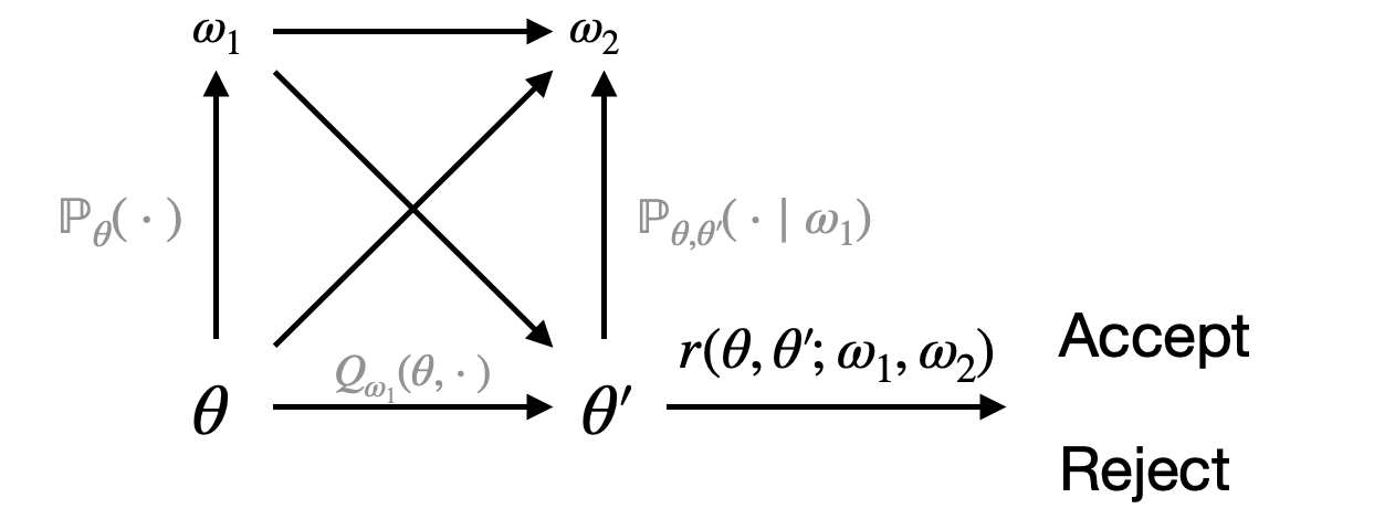
Figure 1: The workflow of Algorithm 4

From now on, we will always assume $\Pi$ is the posterior $\pi(\cdot\mid x)$ without further specification. When both $\Omega_{1}=\Omega_{2}=\mathsf{NULL}$, then no auxiliary variable is generated. Algorithm 4 reduces to the standard Metropolis–Hastings algorithm. We will now briefly discuss a few other possibilities of choosing $\omega_{1}$ and $\omega_{2}$.

Case 1 (Without $\omega_{1}$).

If $\Omega_{1}=\mathsf{NULL}$, Algorithm 4 does not utilise any auxiliary variable for the proposal distribution. The acceptance ratio in Step 6 of Algorithm 4 simplifies to

$$\frac{\pi(\theta^{\prime}\mid x)\mathbb{P}_{\theta^{\prime},\theta_{t}}(\omega_{2})}{\pi(\theta_{t}\mid x)\mathbb{P}_{\theta_{t},\theta^{\prime}}(\omega_{2})}\cdot\frac{q(\theta^{\prime},\theta_{t})}{q(\theta_{t},\theta^{\prime})}.$$

This scenario recovers the previous common procedure discussed in Section 2, which in turn includes the exchange algorithm, PoissonMH, and TunaMH (Algorithm 1, 2, 3).

Case 2 ($\omega_{1}=\omega_{2}$).

Another interesting case is when $\omega_{1}=\omega_{2}$, i.e., the two auxiliary variables are perfectly correlated. In this case, the acceptance ratio reduces to

$$\frac{\pi(\theta^{\prime}\mid x)\mathbb{P}_{\theta^{\prime}}(\omega_{1})}{\pi(\theta_{t}\mid x)\mathbb{P}_{\theta_{t}}(\omega_{1})}\cdot\frac{q_{\omega_{1}}(\theta^{\prime},\theta_{t})}{q_{\omega_{1}}(\theta_{t},\theta^{\prime})}.$$

In this case, $\omega_{1}$ can assist in designing the proposal distribution. This approach can sometimes also help estimate the target ratio and reduce per-iteration costs through careful design, as discussed in Section 3.3.1. This includes the auxiliary Metropolis-Hastings sampler (Section 2.1 of Titsias and Papaspiliopoulos, (2018)) as a special case. However, a potential limitation is that $\omega_{1}$ is generated based solely on the current state $\theta_{t}$. Incorporating information from the proposed state $\theta^{\prime}$ could further improve the target ratio estimator.

Case 3 ($\omega_{1}$ independent with $\omega_{2}$).

When $\omega_{1}$ is independent with $\omega_{2}$, the acceptance ratio can be written as

$$\frac{\pi(\theta^{\prime}\mid x)\mathbb{P}_{\theta^{\prime}}(\omega_{1})\mathbb{P}_{\theta^{\prime},\theta_{t}}(\omega_{2})}{\pi(\theta_{t}\mid x)\mathbb{P}_{\theta_{t}}(\omega_{1})\mathbb{P}_{\theta_{t},\theta^{\prime}}(\omega_{2})}\cdot\frac{q_{\omega_{1}}(\theta^{\prime},\theta_{t})}{q_{\omega_{1}}(\theta_{t},\theta^{\prime})}.$$

Methodologically, this approach addresses the issues of proposal design’ and ‘ratio estimation’ separately. Users can generate one minibatch to guide the proposal and use the other to estimate the target ratio. We will discuss this strategy further in Section 3.3.2. The ratio $\mathbb{P}_{\theta^{\prime}}(\omega_{1})/\mathbb{P}_{\theta_{t}}(\omega_{1})$ will also be cancelled out when the distribution of $\omega_{1}$ does not depend on $\theta$.

3.3 New algorithms

We now introduce new gradient-based minibatch algorithms within our framework (Algorithm 4). We focus on sampling from a tall dataset where $\pi(\theta\mid x)\propto\pi(\theta)p_{\theta}(x)=\pi(\theta)\prod_{i=1}^{N}\mathsf{p}_{\theta}(x_{i})$. Our goal is to incorporate gradient information in the proposal design while maintaining the correct stationary distribution and minimal overhead. Each iteration only requires a minibatch of data. The high-level idea is to introduce an auxiliary variable ($\omega_{1}$ in Algorithm 4) to estimate the full gradient at a low cost. Then, we use a second auxiliary variable $\omega_{2}$, as described in Section 2, to estimate the target ratio. These two variables may be either independent or correlated, depending on the application.

3.3.1 PoissonMH with locally balanced proposal

In this section, we will adhere to all the technical assumptions of PoissonMH (Algorithm 2).
Locally balanced proposal: We first briefly review the idea of the locally balanced proposal. The idea is initially introduced in Zanella, (2020) for discrete samplers and later extended in Livingstone and Zanella, (2022); Vogrinc et al., (2023). It has proven to be a convenient framework for integrating traditional algorithms and developing new algorithms.

The Barker’s proposal in Zanella, (2020) is of the form $Q^{g}(\theta,\mathrm{d}\theta^{\prime})\propto g\left(\pi(\theta^{\prime}\mid x)/\pi(\theta\mid x)\right)K(\theta,\mathrm{d}\theta^{\prime}),$ where $g:\mathbb{R}^{+}\xrightarrow{}\mathbb{R}^{+}$ is a balancing function satisfying $g(t)=tg(1/t)$. Here, $K$ represents a symmetric kernel. Users can choose the balancing function, with recommended options including $g(t)=\sqrt{t}$ and $g(t)=t/(1+t)$. Experiments on various discrete distributions show that its performance is competitive compared to alternative MCMC methods.

When $\theta$ is in a continuous state space, the proposal $Q^{g}(\theta,\cdot)$ is not feasible for implementation. However, one can perform a first–order Taylor expansion of $\log(\pi(\theta^{\prime}\mid x))-\log(\pi(\theta\mid x))$ with respect to $\theta$, and utilise the so-called first-order locally balanced proposal. It has the form: $Q^{(g)}(\theta,\mathrm{d}\theta^{\prime})=\prod_{i=1}^{d}Q^{(g)}_{i}(\theta,\mathrm{d}\theta^{\prime}_{i}).$ Here $Q^{(g)}_{i}$ is a one-dimensional kernel of the form

$$Q^{(g)}_{i}(\theta,\mathrm{d}\theta^{\prime}_{i})=Z^{-1}_{i}(\theta)g\left(e^{\left(\partial_{\theta_{i}}\log\pi(\theta\mid x)\right)(\theta^{\prime}_{i}-\theta_{i})}\right)\mu_{i}(\theta^{\prime}_{i}-\theta_{i})\mathrm{d}\theta_{i}^{\prime}$$ (2)

where $\mu_{i}(\cdot)$ represents a symmetric density in $\mathbb{R}$, such as a centred Gaussian. Livingstone and Zanella, (2022) note that selecting $g(t)=\sqrt{t}$ corresponds to MALA. They suggest using $g(t)=t/(1+t)$, referred to as ‘Barker’s proposal’, inspired by Barker, (1965). This choice allows exact calculation of $Z_{i}(\theta)$, and in turn implies an efficient algorithm for $Q^{(g)}(\theta,\cdot)$. They find that Barker’s proposal tends to be more robust compared to MALA.
Our proposal: We retain all promises and notations used in Algorithm 2. We also use the notation $\omega_{1}:=(s_{1},s_{2},\ldots,s_{N})$ and $\mathbb{P}_{\theta}(\cdot):=\otimes_{i=1}^{N}\mathsf{Poi}\left(\frac{\lambda M_{i}}{L}+\phi_{i}(\theta;x)\right)$, as defined in Example 2. For every balancing function $g$, we define the Markov transition kernels with density $q_{\omega_{1}}^{(g)}(\theta,\theta^{\prime}):=\prod_{i=1}^{d}q_{\omega_{1},i}^{(g)}(\theta,\theta_{i}^{\prime}).$ Here $q_{\omega_{1},i}^{(g)}$ is a one-dimensional density proportional to

$$g\left(e^{\partial_{\theta_{i}}\log\left(\pi(\theta\mid x)\mathbb{P}_{\theta}(\omega_{1})\right)(\theta^{\prime}_{i}-\theta_{i})}\right)\mu_{i}(\theta^{\prime}_{i}-\theta_{i}),$$ (3)

where $\mu_{i}$ is a symmetric density on $\mathbb{R}$. Our algorithm is summarised in Algorithm 5.

Algorithm 5 corresponds to Case 2 of our meta-algorithm 4. Consequently, its validity is directly proven by Proposition 2. Moreover, several points are worth discussing.

Algorithm 5 Locally Balanced PoissonMH

1:  Initialise: Initial state $\theta_{0}$; balancing function $g$; number of iterations $T$

2:  for $t=0$ to $T-1$ do

3:     sample $\omega_{1}=(s_{1},s_{2},\cdots,s_{N})\sim\mathbb{P}_{\theta_{t}}(\cdot)$, form minibatch $S=\{i\mid s_{i}>0\}$

4:     propose $\theta^{\prime}\sim q_{\omega_{1}}^{(g)}(\theta_{t},\cdot)$

5:     compute

$$r\leftarrow\frac{\pi(\theta^{\prime}\mid x)\mathbb{P}_{\theta^{\prime}}(\omega_{1})}{\pi(\theta_{t}\mid x)\mathbb{P}_{\theta_{t}}(\omega_{1})}\cdot\frac{q_{\omega_{1}}^{(g)}(\theta^{\prime},\theta_{t})}{q_{\omega_{1}}^{(g)}(\theta_{t},\theta^{\prime})}.$$

6:     with probability $\min\{1,r\}$, set $\theta_{t+1}\xleftarrow{}\theta^{\prime}$; otherwise, $\theta_{t+1}\xleftarrow{}\theta_{t}$

7:  end for

Firstly, the proposed method is an auxiliary-variable-based variant of the locally-balanced proposal. Our proposal distribution $q_{\omega_{1}}^{(g)}$ closely resembles the first-order locally balanced proposal, with one key modification. The term $\partial_{\theta_{i}}\log\pi(\theta\mid x)$ in (2) is substituted by $\partial_{\theta_{i}}\log\left(\pi(\theta\mid x)\mathbb{P}_{\theta}(\omega_{1})\right)$ in (3). Meanwhile, standard calculation shows the proxy function $\pi(\theta\mid x)\cdot\mathbb{P}_{\theta}(\omega_{1})$ only depends on the minibatch $S$. Consequently, the cost of computing the gradient is at the same level as calculating the acceptance ratio in PoissonMH, thus not significantly increasing the cost per step. Detailed calculations are in supplementary B.

Secondly, our key observation is the auxiliary variable $\omega_{1}$ depends only on the current state $\theta$. Therefore, one may as well first generate the minibatch and then propose the new step, i.e. swap the order of Steps 4 and 5 in Algorithm 2. Then, $\pi(\theta\mid x)\mathbb{P}_{\theta}(\omega_{1})$ is employed as a computationally proxy function. Therefore, the auxiliary variable $\omega_{1}$ is simultaneously used for estimating both the gradient and the target ratio.

Lastly, following Livingstone and Zanella, (2022), we choose $g(t)=t/(1+t)$ and $g(t)=\sqrt{t}$ in our actual implementation. We call them Poisson–Barker and Poisson–MALA respectively. These are the minibatch versions (covering both proposal generation and target ratio evaluation) of the Barker proposal and MALA. Similar to Livingstone and Zanella, (2022), these choices of $g$ allow efficient implementation, with details available in supplementary B. Their numerical performances and comparisons are examined in Section 5.

3.3.2 TunaMH with SGLD proposal

In this section, we will adhere to all the technical assumptions in TunaMH (Algorithm 3). Recall the target distribution has the form $\pi(\theta\mid x)\propto\exp{\{-\sum_{i=1}^{N}U_{i}(\theta;x)\}}$.

A key idea of Algorithm 5 is using the same auxiliary variable for estimating the gradient and target ratio. However, this approach is infeasible for improving TunaMH. As noted in Section 2, the auxiliary variable in TunaMH depends on both the current and proposed states, requiring the new state to be proposed before generating the auxiliary variable.

Therefore, we adopt another cost-effective strategy for utilising the gradient information, inspired by the SGLD algorithm in Welling and Teh, (2011). At each step, we first select a minibatch $B$ of $K$ data points uniformly from the entire dataset. Thus $(N/K)\sum_{i\in B}\nabla_{\theta}U_{i}(\theta_{t};x)$ is a natural estimator of the gradient of the log-posterior: $\nabla_{\theta}\log\pi(\theta\mid x)=-\nabla_{\theta}\sum_{i=1}^{N}U_{i}(\theta;x)$. Calculating this estimator has a cost that scales linearly with the minibatch size $K$, rather than with the total dataset size $N$. In the examples we considered, data size $N$ is no less than $10,000$ while $K$ is often chosen as $20$. Therefore, computing the estimated gradient is significantly cheaper compared to calculating the full gradient. Setting $\omega_{1}:=B\sim\mathsf{Unif}\{\{1,2,\ldots,N\},K\}$, our proposal has the form $q_{\omega_{1}}(\theta,\cdot)\sim\mathbb{N}\left(\theta-\frac{\epsilon^{2}}{2}\frac{N}{K}\sum_{i\in B}\nabla_{\theta}U_{i}(\theta;x),\epsilon^{2}\mathbb{I}\right),$ where $\epsilon$ is a tuning parameter. Next, we use the same strategy as TunaMH to select an independent minibatch to estimate the target ratio. Using the notations $\omega_{2}:=(s_{1},s_{2},\ldots,s_{N})$ and $\mathbb{P}_{\theta,\theta^{\prime}}(\cdot):=\otimes_{i=1}^{N}\mathsf{Poi}\left(\frac{\lambda c_{i}}{C}+\phi_{i}(\theta,\theta^{\prime};x)\right)$, our algorithm is summarised in Algorithm 6.

Algorithm 6 corresponds to Case 3 of our meta-algorithm 4. Thus, its validity directly follows from Proposition 2. Our first auxiliary variable $\omega_{1}$ is independent of the second. Therefore, the distribution $\mathbb{P}_{\theta,\theta^{\prime}}(\cdot\mid\omega_{1})$ equals $\mathbb{P}_{\theta,\theta^{\prime}}(\cdot)$. Additionally, the first variable $\omega_{1}=B$ follows a fixed distribution that does not depend on $\theta$. Consequently, the joint distribution $\mathbb{P}_{\theta,\theta^{\prime}}(\omega_{1},\omega_{2})$ equals $\mathbb{P}(\omega_{1})\mathbb{P}_{\theta,\theta^{\prime}}(\omega_{2})$. As a result, Step 6 of Algorithm 4 simplifies to

$$\frac{\pi(\theta^{\prime}\mid x)\mathbb{P}_{\theta^{\prime},\theta_{t}}(\omega_{2})}{\pi(\theta_{t}\mid x)\mathbb{P}_{\theta_{t},\theta^{\prime}}(\omega_{2})}\cdot\frac{q_{\omega_{1}}(\theta^{\prime},\theta_{t})}{q_{\omega_{1}}(\theta_{t},\theta^{\prime})}.$$

For readers already familiar with SGLD, another natural perspective is to view Algorithm 6 as a minibatch Metropolised version of SGLD. If each iteration of Algorithm 6 skips Steps 5–7 for the acceptance–rejection correction, it becomes exactly the SGLD algorithm described in Welling and Teh, (2011) with a fixed step size. The SGLD algorithm is a noisier but much faster version of the Unadjusted Langevin Algorithm (ULA). Both ULA and SGLD with a fixed step size have systematic bias, as they do not converge to the target distribution $\pi(\theta\mid x)$ even after an infinite number of steps (Vollmer et al.,, 2016). Introducing a straightforward Metropolis–Hastings acceptance–rejection step can ensure the correct stationary distribution but requires full-dataset evaluation, which undermines the advantage of SGLD. Therefore, deriving an acceptance–rejection version of SGLD using minibatch data is considered an open problem. To quote from Welling and Teh, (2011): Interesting directions of future research includes deriving a MH rejection step based on mini-batch data $\ldots$

Algorithm 6 offers a solution to this problem under the same assumptions as Algorithm 3. It eliminates the systematic bias in SGLD by incorporating an acceptance–rejection step based on the approach used in TunaMH. Relaxing the technical assumptions or generalizing to posterior distributions with non-i.i.d. model likelihoods are intriguing open questions.

Algorithm 6 TunaMH–SGLD

1:  Initialise: Initial state $\theta_{0}$; batch size $K$; step size $\epsilon$; number of iterations $T$

2:  for $t=0$ to $T-1$ do

3:     sample the first minibatch $B\subset\{1,2,\cdots,N\}$ uniformly at random with size $K$

4:     propose $\theta^{\prime}\sim q_{\omega_{1}}(\theta_{t},\cdot)$

5:     sample $\omega_{2}=(s_{1},s_{2},\cdots,s_{N})\sim\mathbb{P}_{\theta_{t},\theta^{\prime}}(\cdot)$, form the second minibatch $S=\{i\mid s_{i}>0\}$

6:     compute

$$r\xleftarrow{}\frac{\pi(\theta^{\prime}\mid x)\mathbb{P}_{\theta^{\prime},\theta_{t}}(\omega_{2})}{\pi(\theta_{t}\mid x)\mathbb{P}_{\theta_{t},\theta^{\prime}}(\omega_{2})}\cdot\frac{q_{\omega_{1}}(\theta^{\prime},\theta_{t})}{q_{\omega_{1}}(\theta_{t},\theta^{\prime})}.$$

7:     with probability $\min\{1,r\}$, set $\theta_{t+1}\xleftarrow{}\theta^{\prime}$; otherwise $\theta_{t+1}\xleftarrow{}\theta_{t}$

8:  end for

4 Theory

This section presents our theoretical analysis. We will begin by examining the meta-algorithm 4 and then apply our findings to specific algorithms. Proposition 2 has already shown the reversibility of the proposed method. Therefore, this section will focus on understanding the convergence speed. Our agenda is to compare the Markov chain in Algorithm 4, with transition kernel denoted by $\mathbb{P}_{\mathsf{aux}}$ with two relevant chains $\mathbb{P}_{\mathsf{ideal}}$ and $\mathbb{P}_{\mathsf{MwG}}$. These two chains need not be implementable, but are easier to study as a stochastic process.

Fix $\theta\in\Theta$, define the idealised proposal $Q_{\mathsf{ideal}}(\theta,\mathrm{d}\theta^{\prime}):=\mathbb{E}_{\omega_{1}\sim\mathbb{P}_{\theta}}[Q_{\omega_{1}}(\theta,\mathrm{d}\theta^{\prime})]$, with density $q_{\mathsf{ideal}}(\theta,\theta^{\prime})=\int_{\Omega_{1}}q_{\omega_{1}}(\theta,\theta^{\prime})\mathbb{P}_{\theta}(\omega_{1})\lambda_{1}(\mathrm{d}\omega_{1})$. The idealised chain $\mathbb{P}_{\mathsf{ideal}}$ refers to the standard Metropolis-Hastings algorithm with proposal $Q_{\mathsf{ideal}}$. Detailed description of $\mathbb{P}_{\mathsf{ideal}}$ is given in Algorithm 7 in supplementary A.4. The second chain, $\mathbb{P}_{\mathsf{MwG}}$, is defined as the transition kernel for Case 2, i.e., $\omega_{1}=\omega_{2}$ in Algorithm 4. A crucial feature is that $\mathbb{P}_{\mathsf{MwG}}$ can equivalently be viewed as a Metropolis–within–Gibbs algorithm. It is the marginal chain for the $\theta$ component, targeting an augmented distribution $\pi(\theta,\omega_{1}\mid x):=\pi(\theta\mid x)\mathbb{P}_{\theta}(\omega_{1})$. At each step, users first generate $\omega_{1}$ from $\pi(\cdot\mid\theta,x)=\mathbb{P}_{\theta}(\cdot)$. They then use the proposal $q_{\omega_{1}}(\theta,\cdot)$ to draw $\theta^{\prime}$, targeting $\pi(\theta^{\prime}\mid\omega_{1},x)\propto\pi(\theta^{\prime}\mid x)\mathbb{P}_{\theta}(\omega_{1})$, and implement an acceptance–rejection step. This perspective allows us to apply recent results, such as Qin et al., (2023), in our analysis.

For each $\theta$, all of $\mathbb{P}_{\mathsf{ideal}}(\theta,\cdot),\mathbb{P}_{\mathsf{MwG}}(\theta,\cdot)$ and $\mathbb{P}_{\mathsf{aux}}(\theta,\cdot)$ can be represented as a mixture of a continuous density on $\Theta$ (with respect to the base measure) and a point mass at $\theta$. We therefore define $p_{\mathsf{ideal}}(\theta,\cdot),p_{\mathsf{MwG}}(\theta,\cdot)$ and $p_{\mathsf{aux}}(\theta,\cdot)$ for the density part, respectively.

4.1 Peskun’s ordering

The following result generalises existing results that use only one auxiliary variable, such as Lemma 1 in Wang, (2022), Section 2.3 in Nicholls et al., (2012), and Section 2.1 in Andrieu et al., 2018a . Nevertheless, the proof idea is very similar and is given in supplementary 4.1.

Lemma 1.

For each pair $(\theta,\theta^{\prime})$ such that $\theta\neq\theta^{\prime}$, $p_{\mathsf{aux}}(\theta,\theta^{\prime})\leq p_{\mathsf{MwG}}(\theta,\theta^{\prime})\leq p_{\mathsf{ideal}}(\theta,\theta^{\prime}).$

This lemma shows that $\mathbb{P}_{\mathsf{aux}}$ is always less likely to move compared to $\mathbb{P}_{\mathsf{ideal}}$ and $\mathbb{P}_{\mathsf{MwG}}$. Lemma 1 implies $\mathbb{P}_{\mathsf{aux}}\prec\mathbb{P}_{\mathsf{MwG}}\prec\mathbb{P}_{\mathsf{ideal}}$ according to Peskun’s ordering (Peskun,, 1973). This means $\mathbb{P}_{\mathsf{MwG}}-\mathbb{P}_{\mathsf{aux}}$ and $\mathbb{P}_{\mathsf{ideal}}-\mathbb{P}_{\mathsf{MwG}}$ are non-negative operators, and the asymptotic variance for any $f$ under $\mathbb{P}_{\mathsf{ideal}}$ is no greater than under $\mathbb{P}_{\mathsf{aux}}$. For more results, see Tierney, (1998).

4.2 Comparing the transition density

Section 4.1 states that Algorithm 4 is statistically less efficient than $\mathbb{P}_{\mathsf{MwG}}$ and $\mathbb{P}_{\mathsf{ideal}}$ due to the “price” paid for the extra auxiliary variables and the cost savings. However, it is more interesting to examine when Algorithm 4 retains most of the efficiency of its counterparts.

We use the shorthand notation $d_{\sf TV}(\theta,\theta^{\prime},\omega_{1}):=d_{\sf TV}\left(\mathbb{P}_{\theta,\theta^{\prime}}(\omega_{2}\mid\omega_{1}),\mathbb{P}_{\theta^{\prime},\theta}(\omega_{2}\mid\omega_{1})\right)$. We also define $d_{\sf TV}(\theta,\theta^{\prime})=\sup_{\omega_{1}}d_{\sf TV}(\theta,\theta^{\prime},\omega_{1})$. Moreover, define the largest KL-divergence $\tilde{d}_{\sf KL}(\theta,\theta^{\prime}):=\sup_{\omega_{1}}d_{\sf KL}\left(\mathbb{P}_{\theta,\theta^{\prime}}(\omega_{2}\mid\omega_{1})||\mathbb{P}_{\theta^{\prime},\theta}(\omega_{2}\mid\omega_{1})\right)$, and its symmetrised version $d_{\sf KL}(\theta,\theta^{\prime}):=0.5\sup_{\omega_{1}}\left(d_{\sf KL}\left(\mathbb{P}_{\theta,\theta^{\prime}}(\omega_{2}\mid\omega_{1})||\mathbb{P}_{\theta^{\prime},\theta}(\omega_{2}\mid\omega_{1})\right)+d_{\sf KL}\left(\mathbb{P}_{\theta^{\prime},\theta}(\omega_{2}\mid\omega_{1})||\mathbb{P}_{\theta,\theta^{\prime}}(\omega_{2}\mid\omega_{1})\right)\right).$

We have the following comparison result on transition density between $p_{\mathsf{aux}}$ and $p_{\mathsf{MwG}}$.

Theorem 1.

For each pair $(\theta,\theta^{\prime})$ such that $\theta\neq\theta^{\prime}$, we have

$$p_{\mathsf{aux}}(\theta,\theta^{\prime}) \geq\left(1-d_{\sf TV}(\theta,\theta^{\prime})\right)p_{\mathsf{MwG}}(\theta,\theta^{\prime})$$

$$\geq e^{-1/e}\exp\{-\min\{d_{\sf KL}(\theta,\theta^{\prime}),\tilde{d}_{\sf KL}(\theta,\theta^{\prime}),\tilde{d}_{\sf KL}(\theta^{\prime},\theta)\}\}p_{\mathsf{MwG}}(\theta,\theta^{\prime}).$$

The following corollaries may be useful when working on specific algorithms.

Corollary 1.

In the following categories, we have:

1. When $\omega_{1}=\mathsf{Null}$, we have $\mathbb{P}_{\mathsf{MwG}}=\mathbb{P}_{\mathsf{ideal}}$ and $Q_{\mathsf{ideal}}=Q_{\mathsf{aux}}$.

2. When $\omega_{1}=\omega_{2}$, then $d_{\sf TV}(\theta,\theta^{\prime})=0$, and $\mathbb{P}_{\mathsf{aux}}=\mathbb{P}_{\mathsf{MwG}}$.

3. When $\omega_{2}$ is independent of $\omega_{1}$, the distribution $\mathbb{P}_{\theta,\theta^{\prime}}(\omega_{2}\mid\omega_{1})$ simplifies to $\mathbb{P}_{\theta,\theta^{\prime}}(\omega_{2})$. Consequently, $d_{\sf TV}(\theta,\theta^{\prime},\omega_{1})$ is constant with respect to $\omega_{1}$ and equals $d_{\sf TV}(\theta,\theta^{\prime})$.

As specific examples, Algorithms 1, 2, and 3 all fall under the first category. The newly introduced Algorithm 5 belongs to the second , while Algorithm 6 belongs to the third.

4.3 Spectral gap

We begin by a concise review of definitions. Consider $P$ as the transition kernel for a Markov chain with stationary distribution $\Pi$. The linear space $L^{2}(\Pi)$ includes all functions $f$ satisfying $\int f^{2}(x)\Pi(\mathrm{d}x)<\infty$. Within this space, $L^{2}_{0}(\Pi)$ is the subspace of functions $f\in L^{2}(\Pi)$ satisfying $\int f(x)\Pi(\mathrm{d}x)=0$. Both $L^{2}(\Pi)$ and $L^{2}_{0}(\Pi)$ are Hilbert spaces with the inner product $\langle f,g\rangle_{\Pi}:=\int(fg)\mathrm{d}\Pi=\mathbb{E}_{\Pi}[fg]$. The norm of $f\in L^{2}(\Pi)$ is $\lVert f\rVert_{\Pi}:=\sqrt{\langle f,f\rangle_{\Pi}}$. The kernel $P$ operates as a linear operator on $L^{2}_{0}(\Pi)$, acting on $f$ by $(Pf)(x):=\int P(x,\mathrm{d}y)f(y)$. Its operator norm on $L^{2}_{0}(\Pi)$ is defined as $\lVert P\rVert_{L^{2}_{0}(\Pi)}:=\sup_{f\in L^{2}_{0}(\Pi),\lVert f\rVert_{\Pi}=1}\lVert Pf\rVert_{\Pi}$. It is known that $\lVert P\rVert_{L^{2}_{0}(\Pi)}\leq 1$. The spectral gap of $P$, denoted as ${\mathsf{Gap}}(P)$, is $1-\lVert P\rVert_{L^{2}_{0}(\Pi)}$.

The next proposition studies the ${\mathsf{Gap}}(\mathbb{P}_{\mathsf{aux}})$, with proof given in supplementary A.7.

Theorem 2.

Let $\Pi=\pi(\theta\mid x)$ be the common stationary distribution of $\mathbb{P}_{\mathsf{MwG}}$ and $\mathbb{P}_{\mathsf{aux}}$. We have ${\mathsf{Gap}}(\mathbb{P}_{\mathsf{aux}})\geq(1-\sup_{\theta,\theta^{\prime}}d_{\sf TV}(\theta,\theta^{\prime})){\mathsf{Gap}}(\mathbb{P}_{\mathsf{MwG}}).$ Similarly, we have ${\mathsf{Gap}}(\mathbb{P}_{\mathsf{aux}})\geq\left(e^{-1/e}\exp\{-\min\{d_{\sf KL}(\theta,\theta^{\prime}),\tilde{d}_{\sf KL}(\theta,\theta^{\prime}),\tilde{d}_{\sf KL}(\theta^{\prime},\theta)\}\}\right){\mathsf{Gap}}(\mathbb{P}_{\mathsf{MwG}}).$:

For an initial distribution $\pi_{0}$ that is $\beta$-warm with respect to the stationary distribution $\Pi$ (i.e., $\pi_{0}(A)/\Pi(A)\leq\beta$ for any $A$), a Markov chain $P$ starting from a $\beta$-warm distribution reaches within $\epsilon$ of the stationary distribution in both total-variation and $L^{2}$ distance after ${\mathcal{O}}(\log(\beta\epsilon^{-1})/{\mathsf{Gap}}(P))$ iterations, as shown in Theorem 2.1 of Roberts and Rosenthal (1997). Theorem 2 states that $\mathbb{P}_{\mathsf{aux}}$ is at most $1/(1-\sup_{\theta,\theta^{\prime}}d_{\sf TV}(\theta,\theta^{\prime}))$ times slower than $\mathbb{P}_{\mathsf{MwG}}$ in terms of iteration count. Conversely, if the per-iteration cost of $\mathbb{P}_{\mathsf{aux}}$ is less than $1/(1-\sup_{\theta,\theta^{\prime}}d_{\sf TV}(\theta,\theta^{\prime}))$ times the cost of $\mathbb{P}_{\mathsf{MwG}}$, then $\mathbb{P}_{\mathsf{aux}}$ is provably more efficient than $\mathbb{P}_{\mathsf{MwG}}$.

Bounding ${\mathsf{Gap}}(\mathbb{P}_{\mathsf{MwG}})$: Given the relationship between ${\mathsf{Gap}}(\mathbb{P}_{\mathsf{aux}})$ and ${\mathsf{Gap}}(\mathbb{P}_{\mathsf{MwG}})$ in Theorem 2, the next step is to bound ${\mathsf{Gap}}(\mathbb{P}_{\mathsf{MwG}})$. We now discuss recent findings from Qin et al., (2023). In each iteration, the chain $\mathbb{P}_{\mathsf{MwG}}$ first draws $\omega_{1}\sim\mathbb{P}_{\theta}(\cdot)$, followed by a Metropolis–Hastings algorithm to sample from $\pi(\theta\mid\omega_{1},x)\propto\pi(\theta\mid x)\mathbb{P}_{\theta}(\omega_{1})$ using the proposal $q_{\omega_{1}}(\theta,\cdot)$. We use $\mathbb{P}_{\mathsf{MHG},\omega_{1}}$ to denote the transition kernel of the second step. We also use $\mathbb{P}_{\mathsf{Gibbs}}$ to denote the “$\theta$-chain” of the standard Gibbs sampler targeting $\pi(\theta\mid x)\mathbb{P}_{\theta}(\omega_{1})$. This means we first draw $\omega_{1}\sim\mathbb{P}_{\theta}(\cdot)$, and then draw $\theta$ directly from $\pi(\theta\mid\omega_{1},x)$.

Proposition 3 (Corollary 14 and Theorem 15 of Qin et al., (2023)).

We have:

1. ${\mathsf{Gap}}(\mathbb{P}_{\mathsf{MwG}})\geq{\mathsf{Gap}}(\mathbb{P}_{\mathsf{Gibbs}})\times\inf_{\omega_{1}}{\mathsf{Gap}}(\mathbb{P}_{\mathsf{MHG},\omega_{1}})$

2. Suppose there is a function $\gamma_{1}:\Omega_{1}\rightarrow[0,1]$ satisfying $\lVert\mathbb{P}_{\mathsf{MHG},\omega_{1}}\rVert_{L^{2}_{0}(\pi(\cdot\mid\omega_{1},x))}\leq\gamma_{1}(\omega_{1})$ for every $\omega_{1}$. Meanwhile $\int\gamma_{1}(\omega_{1})^{t}\mathbb{P}_{\theta}(\mathrm{d}\omega_{1})\leq\alpha_{t}$ for every $\theta$ and some even $t$. Then ${\mathsf{Gap}}(\mathbb{P}_{\mathsf{MwG}})\geq t^{-1}\left({\mathsf{Gap}}(\mathbb{P}_{\mathsf{Gibbs}})-\alpha_{t}\right)$

The first result is known in Andrieu et al., 2018b . The second result generalises the results of Łatuszyński and Rudolf, (2014). They have been applied in analysing proximal samplers and hybrid slice samplers. See Section 5 of Qin et al., (2023) for details.

4.4 Applications to existing algorithms

We will explain how Theorem 1 and Theorem 2 can be applied to study current algorithms.

Exchange algorithm: Since the exchange algorithm (Algorithm 2) has $\omega_{1}=\mathsf{Null}$, we know $\mathbb{P}_{\mathsf{MwG}}=\mathbb{P}_{\mathsf{ideal}}$. Our next proposition recovers Theorem 5 in Wang, (2022).

Proposition 4.

Let $\mathbb{P}_{\mathsf{aux}}$ be the transition kernel of Algorithm 1, then we have $p_{\mathsf{aux}}(\theta,\theta^{\prime})\geq\left(1-\sup_{\theta,{\theta^{\prime}}}d_{\sf TV}(p_{\theta},p_{\theta^{\prime}})\right)p_{\mathsf{ideal}}(\theta,\theta^{\prime}).$ Let $A_{\theta,\theta^{\prime}}(s):=\{\omega:p_{\theta}(\omega)>sp_{\theta^{\prime}}(\omega)\}$. If there exists $\epsilon,\delta\in(0,1)$ such that $\mathbb{P}_{p_{\theta^{\prime}}}(A_{\theta,\theta^{\prime}}(\delta))>\epsilon$ uniformly over $\theta,\theta^{\prime}$, then ${\mathsf{Gap}}(\mathbb{P}_{\mathsf{aux}})\geq\epsilon\delta{\mathsf{Gap}}(\mathbb{P}_{\mathsf{ideal}})$.

PoissonMH: Theorem 2 allows us to give a (arguably) simpler proof for the theoretical analysis of PoissonMH, with slightly stronger results. The proof is in supplementary A.9.

Proposition 5.

With all the notations used in PoissonMH, let $\mathbb{P}_{\mathsf{aux}}$ be the transition kernel of Algorithm 2. Then we have ${\mathsf{Gap}}(\mathbb{P}_{\mathsf{aux}})\geq e^{-1/e}\exp\left\{\frac{-L^{2}}{\max\{\lambda+L,2\lambda\}}\right\}{\mathsf{Gap}}(\mathbb{P}_{\mathsf{ideal}})$.

Theorem 2 of Zhang and De Sa, (2019) establishes ${\mathsf{Gap}}(\mathbb{P}_{\mathsf{aux}})\geq 0.5\exp\left\{\frac{-L^{2}}{\lambda+L}\right\}{\mathsf{Gap}}(\mathbb{P}_{\mathsf{ideal}})$ as the main theoretical guarantee for PoissonMH. Our exponent term $\frac{-L^{2}}{\max\{\lambda+L,2\lambda\}}$ is always at least as good as theirs, and is strictly shaper if $\lambda>L$. For example, the suggested choice of $\lambda$ is of the order $L^{2}$ (with $L$ being approximately of the order $N$) in the original paper, which satisfies this requirement. Our constant $e^{-1/e}\approx 0.69$ is also slightly than their $0.5$.

TunaMH: As another application of Theorem 2, we provide a (again, arguably) simpler proof for TunaMH, achieving stronger results. The proof is in supplementary A.10.

Proposition 6.

With all the notations used in TunaMH (Algorithm 3), let $\mathbb{P}_{\mathsf{aux}}$ be the transition kernel of Algorithm 3. Then we have ${\mathsf{Gap}}(\mathbb{P}_{\mathsf{aux}})\geq e^{-1/e}\exp\left\{-1/2\chi\right\}{\mathsf{Gap}}(\mathbb{P}_{\mathsf{ideal}})$.

Theorem 2 of Zhang et al., (2020) shows ${\mathsf{Gap}}(\mathbb{P}_{\mathsf{aux}})\geq\exp\{-1/\chi-2\sqrt{(\log 2)/\chi}\}{\mathsf{Gap}}(\mathbb{P}_{\mathsf{ideal}})$. Our rate $\exp\{-1/2\chi\}$ is strictly sharper than theirs, with the improvement increasing as $\chi$ decreases. Although our constant $e^{-1/e}$ is about 30% worse, the tuning parameter $\chi$, which controls the expected batch size, is often very small (e.g., $10^{-4}$ or $10^{-5}$ in Section 5 of Zhang et al., (2020)). In those cases, our bound is approximately $\exp(10^{4})$ or $\exp(10^{5})$ times sharper.

4.5 From algorithms to a more powerful theory, and back

Theorem 2 offers valuable insights for existing algorithms but has significant limitations due to its assumptions. It provides non-trivial lower bounds on the spectral gap only when $\sup_{\theta,\theta^{\prime}}d_{\sf TV}(\theta,\theta^{\prime})<1$. This condition is met by PoissonMH and TunaMH (implicitly), but may not hold in many practical cases. Conversely, the ‘pointwise’ comparison (Theorem 1) is more robust. An appealing research direction is to establish a weaker version of Theorem 2 under relaxed assumptions. Promising approaches include using approximate conductance (Dwivedi et al.,, 2019; Ascolani et al.,, 2024) and weak Poincaré inequalities (Andrieu et al.,, 2022, 2023). These methods have recently shown success in MCMC algorithm analysis. For instance, weak Poincaré inequalities can provide useful bounds on the mixing time for pseudo-marginal MCMC when the spectral gap of the idealised chain is unknown or nonexistent.

A more powerful comparison theory could also lead to new algorithms with theoretical guarantees. As shown in Section 4.4, the assumptions in Zhang and De Sa, (2019) and Zhang et al., (2020) implicitly imply the stringent condition $\sup_{\theta,\theta^{\prime}}d_{\sf TV}(\theta,\theta^{\prime})<1$. Thus, developing a new theory with relaxed assumptions might lead to algorithms with broader applicability.

5 Numerical experiments

This section presents numerical experiments. We first examine two simulated examples: heterogeneous truncated Gaussian and robust linear regression. We compare our Poisson–Barker and Poisson–MALA algorithms with PoissonMH and full batch algorithms like random-walk Metropolis, MALA, and HMC. In the third experiment, we apply Bayesian logistic regression on the MNIST dataset, comparing TunaMH–SGLD with TunaMH, random-walk Metropolis, MALA, and HMC. Our results show that our gradient-based minibatch methods significantly outperform existing minibatch and full-batch methods.

We implement all methods in Julia. The reproducible code is at https://github.com/ywwes26/MCMC-Auxiliary. In all the figures in this section, the random-walk Metropolis is labeled as MH, while all other methods are labeled by their respective names. Different minibatch algorithms require prior knowledge of different bounds on the model likelihood (refer to the “promise” block in Algorithm 2 and 3). They are derived in supplementary D.

5.1 Heterogeneous truncated Gaussian

We begin with an illustration example. Suppose $\theta\in\mathbb{R}^{d}$ is our parameter of interest, the data $\{y_{i}\}_{i=1}^{N}$ is generated i.i.d. from $y_{i}\mid\theta\sim\mathbb{N}(\theta,\Sigma)$ with $\theta=(0,0,\ldots,0)$. In our experiment, we set $d=20$, $N=10^{5}$, $\beta=10^{-5}$ and $\Sigma=\text{Diagonal}(1,0.95,0.90,\cdots,0.05)$. Therefore, our data follows a multidimensional heterogeneous Gaussian, a common setting in sampling tasks such as Neal et al., (2011). Following Zhang and De Sa, (2019); Zhang et al., (2020), we truncate the parameter $\theta$ to a hypercube $[-3,3]^{d}$ and apply a flat prior. As in Seita et al., (2018); Zhang et al., (2020), we aim to sample from the tempered posterior: $\pi(\theta\mid\{y_{i}\}_{i=1}^{N})\propto\exp\left\{-\frac{1}{2}\beta\sum_{i=1}^{N}(\theta-y_{i})^{\intercal}\Sigma^{-1}(\theta-y_{i})\right\}$ with $\beta=10^{-5}$.

We test PoissonMH, Poisson–MALA, Poisson–Barker, (full batch) random-walk Metropolis, and (full batch) MALA. Following Zhang and De Sa, (2019), the hyperparameter $\lambda$ for the three minibatch algorithms is set to $\lambda=0.0005L^{2}$, resulting in a batch size of about 6000 (6% of the data points). The initial $\theta_{0}$ is drawn from $\mathbb{N}(0,\mathbb{I}_{d})$, and each algorithm’s step size is tuned through several pilot runs to achieve target acceptance rates of 0.25, 0.4, and 0.55. We use Mean Squared Error (MSE) and Effective Sample Size (ESS) to compare these methods. MSEs are calculated for estimating the posterior mean and variance, with true values computed numerically. ESS quantifies the dependence of MCMC samples, with each dimension corresponding to an ESS in an MCMC run. We report the minimum, median, and maximum ESS across all dimensions for all methods.

We compare the clock-time performances of the five methods. Figure 2 shows the MSE over time at different acceptance rates. We find: 1. Poisson–Barker significantly improves PoissonMH, random-walk Metropolis, and MALA for all acceptance rates, both in terms of posterior mean and variance, with more notable improvement at higher acceptance rates. 2. All three minibatch algorithms (PoissonMH, Poisson–MALA, Poisson–Barker) consistently outperform random-walk Metropolis and MALA, demonstrating their effectiveness in the tall data regime. 3. Poisson–MALA matches Poisson–Barker’s best performance at acceptance rates of 0.4 and 0.55 but shows fluctuations and slightly worse performance than PoissonMH at a 0.25 acceptance rate, aligning with Livingstone and Zanella, (2022) that MALA is sensitive to tuning, while Barker’s proposal is more robust.

Table 1 compares ESS per second (ESS/s) across various acceptance rates. Our gradient-based minibatch methods, Poisson–Barker and Poisson–MALA, consistently rank as the top two methods for all acceptance rates (0.25, 0.4, 0.55) and metrics (min, median, max) ESS/s. They improve performance by $1.24-7.02$ times over PoissonMH, $7.61-12.33$ times over MALA, and $13.00-67.24$ times over random-walk Metropolis. At a 0.25 acceptance rate, Poisson-Barker performs best, closely followed by Poisson-MALA. At a 0.55 acceptance rate, Poisson–MALA achieves the highest performance, which is also the highest overall performance when all methods are optimally tuned. At a 0.4 acceptance rate, Poisson–Barker and Poisson–MALA are comparable. Despite the additional gradient estimations, our gradient-based algorithms show substantial benefits from a more efficient proposal.

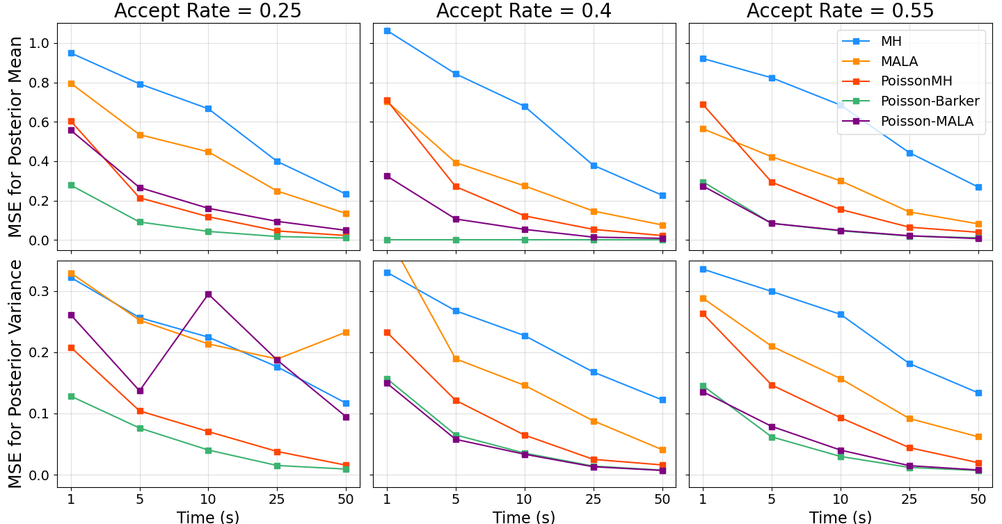
Figure 2: Clock-wise MSE comparison. First row: MSE of posterior mean as a function of time for different acceptance rates; Second row: MSE of posterior variance as a function of time for different acceptance rates. The results are averaged over 10 runs for all five methods.

ESS/s: (Min, Median, Max) Method acceptance rate=0.25 acceptance rate=0.4 acceptance rate=0.55 Best MH (0.04, 0.06, 0.40) (0.03, 0.04, 0.41) (0.03, 0.04, 0.33) (0.04, 0.06, 0.41) MALA (0.06, 0.11, 0.68) (0.09, 0.18, 1.57) (0.09, 0.15, 2.57) (0.09, 0.18, 2.57) PoissonMH (0.37, 0.64, 4.55) (0.31, 0.48, 3.99) (0.25, 0.39, 3.16) (0.37, 0.64, 4.55) Poisson–Barker (0.74, 1.32, 5.77) (0.74, 1.40, 8.38) (0.79, 1.45, 10.68) (0.79, 1.45, 10.68) Poisson–MALA (0.52, 1.09, 5.64) (0.73, 1.37, 12.87) (0.81, 1.53, 22.19) (0.81, 1.53, 22.19)

Table 1: ESS/s comparison. Here (Min, Median, Max) refer to the minimum, median and maximum of ESS/s across all dimensions. The column “Best” reports the best ESS/s across all acceptance rates. The results are averaged over 10 runs for all five methods.

5.2 Robust linear regression

We compare Poisson-Barker, Poisson-MALA, PoissonMH, random-walk Metropolis, MALA, and HMC in a robust linear regression example, as considered in Cornish et al., (2019); Zhang et al., (2020); Maclaurin and Adams, (2014). The data is generated following previous works: for $i=1,2,\cdots,N$, covariates $x_{i}\in\mathbb{R}^{d}$ are independently generated from $\mathbb{N}(0,\mathbb{I}_{d})$ and $y_{i}=\sum_{j=1}^{d}x_{ij}+\epsilon_{i}$ with $\epsilon_{i}\sim\mathbb{N}(0,1)$. The likelihood is modeled as $p(y_{i}\mid\theta,x_{i})=\text{Student}(y_{i}-\theta^{\intercal}x_{i}\mid v)$, where $\text{Student}(\cdot\mid v)$ is the density of a Student’s t distribution with $v$ degrees of freedom. The model is “robust” due to the heavier tail of the likelihood function Maclaurin and Adams, (2014). With a flat prior, the tempered posterior is: $\pi(\theta\mid\{y_{i},x_{i}\}_{i=1}^{N})\propto\exp\left\{-\beta\cdot\frac{v+1}{2}\sum_{i=1}^{N}\log\left(1+\frac{(y_{i}-\theta^{\intercal}x_{i})^{2}}{v}\right)\right\}.$

When the data is appropriately re-scaled (e.g., each covariate has a mean of 0 and variance of 1), the regression coefficient is typically restricted to a certain range. Therefore, we follow the common practice (Gelman et al.,, 2008) of constraining the coefficients within a high-dimensional sphere $\{\theta\in\mathbb{R}^{d}\mid\|\theta\|_{2}\leq R\}$, which has a similar effect to $l^{2}$-regularization.

We use $v=4$ as in Cornish et al., (2019); Zhang et al., (2020) and set $d=10$, $N=10^{5}$, $\beta=10^{-4},R=15$. PoissonMH, Poisson–MALA and Poisson–Barker use $\lambda=0.01L^{2}$. A $50$ dimensional example is in supplementary E.2. The number of leapfrog steps in HMC is set to $10$. The initial $\theta_{0}$ is drawn from $\mathbb{N}(0,\mathbb{I}_{d})$, and the step size of each algorithm is tuned to achieve acceptance rates of $0.25,0.4,$ and $0.55$. Our true parameter is $\theta^{\star}=(1,1,\ldots,1)$.

Figure 3 shows the MSE of estimating the true coefficients over time. Poisson–MALA and Poisson–Barker are much more efficient than PoissonMH, and all minibatch methods outperform full-batch methods. Poisson–MALA and Poisson–Barker adapt to the posterior faster due to gradient information. For example, in Figure 3 (a), Poisson–MALA and Poisson–Barker have an MSE much less than 0.25 at 0.05 seconds, whereas PoissonMH is around 0.5. Full-batch methods adapt slowly because they require a complete dataset scan. MALA outperforms random-walk Metropolis when properly tuned. HMC performs worse than MALA and sometimes even worse than random-walk Metropolis due to the high cost of its $10$ leapfrog steps, making it about $20$ times more costly.

We also present the ESS/s comparisons in Table 2. The results have a similar trend to Section 5.1. Poisson–MALA and Poisson–Barker are the top two methods across all metrics, showing improvements ranging from 2.61 to 4.62 times over PoissonMH, and achieving nearly or more than 100 times the performance of full-batch methods.

Supplementary E.1 presents additional experiments that compare different HMC leapfrog steps and MSE over the iteration count. Supplementary E.2 considers a 50-dimensional robust linear regression with other settings unchanged, yielding similar conclusions.

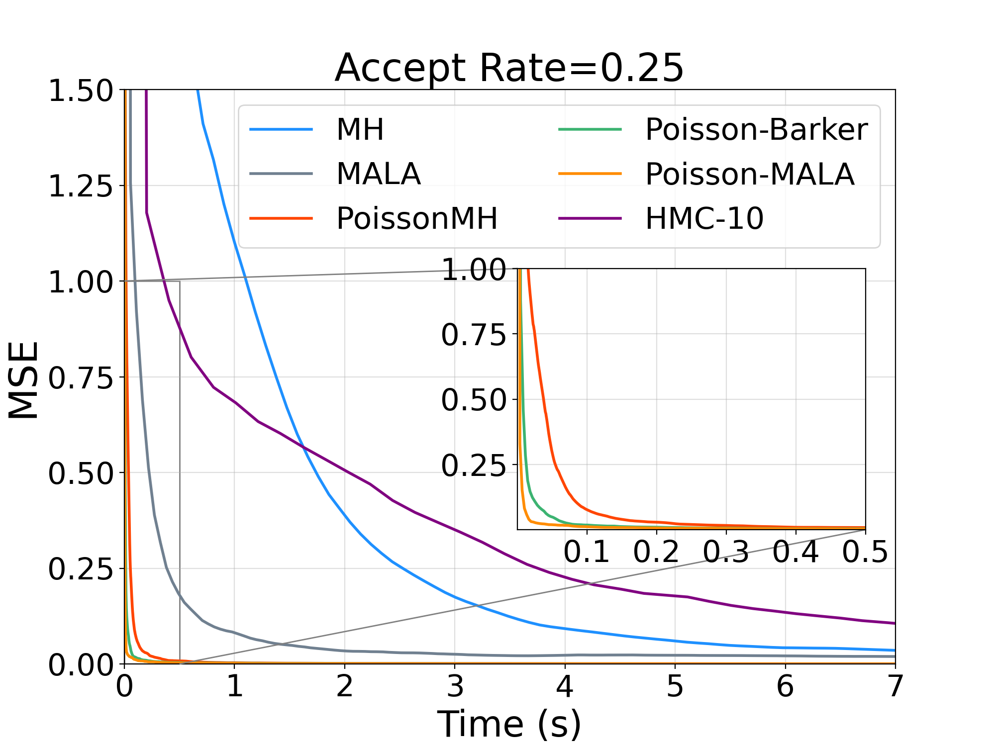
(a) acceptance rate=0.25

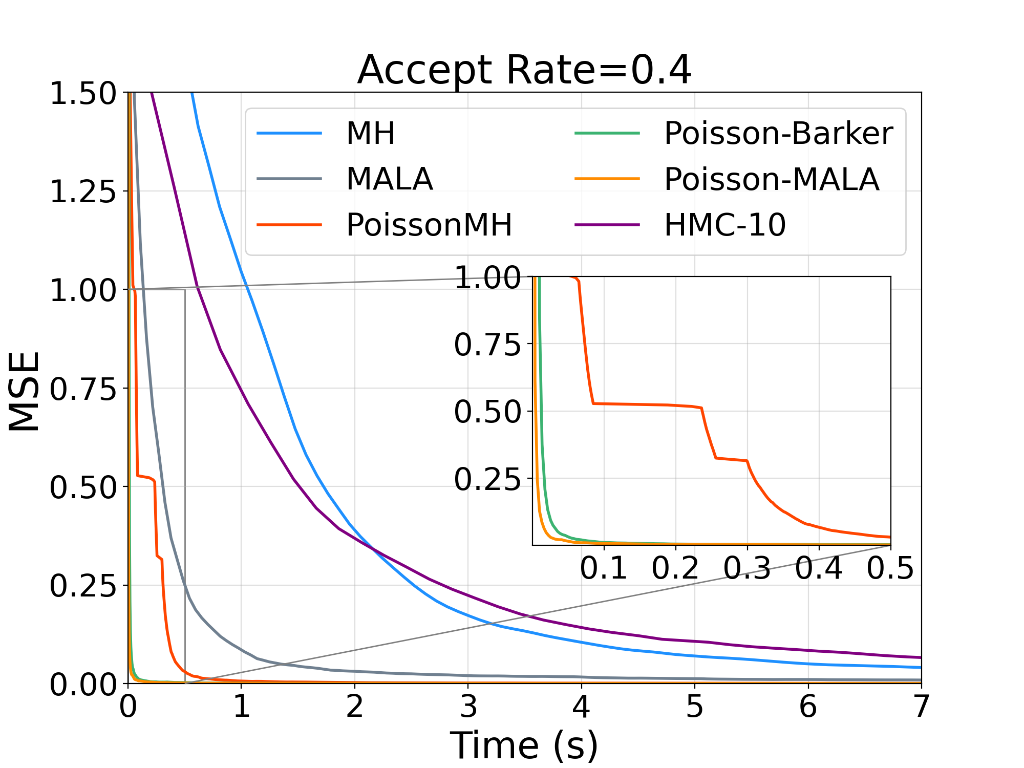
(b) acceptance rate=0.4

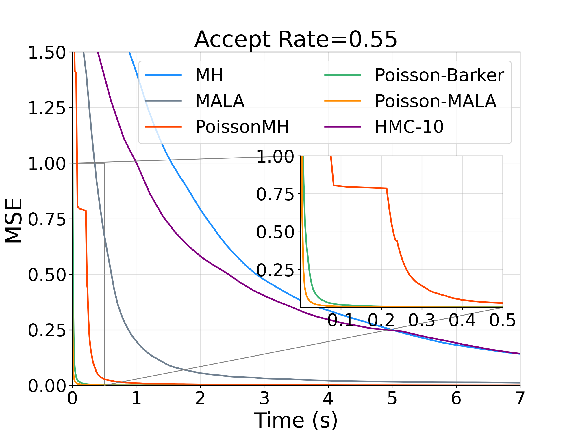
(c) acceptance rate=0.55

Figure 3: Clock-wise MSE comparison. MSE of $\theta^{\star}$ as a function of time across different acceptance rates. The three large plots show the performance of all methods in the first 7 seconds. The three inside plots zoom in on PoissonMH, Poisson-Barker, and Poisson-MALA in the first 0.5 seconds. All results are averaged over 10 runs.

ESS/s: (Min, Median, Max) Method acceptance rate=0.25 acceptance rate=0.4 acceptance rate=0.55 Best MH (1.3, 1.6, 1.8) (1.3, 1.5, 1.7) (0.9, 1.0, 1.1) (1.3, 1.6, 1.8) MALA (1.6, 1.7, 1.8) (3.3, 3.6, 3.8) (3.8, 4.1, 4.3) (3.8, 4.1, 4.3) HMC-10 (0.6, 0.7, 0.7) (0.7, 0.8, 0.8) (0.7, 0.8, 0.8) (0.7, 0.8, 0.8) PoissonMH (73.7, 76.7, 79.5) (66.2, 68.6, 70.7) (41.4, 44.4, 46.3) (73.7, 76.7, 79.5) PoissonMH-Barker (135.5, 142.0, 145.0) (195.1, 199.1, 206.9) (197.4, 204.3, 207.7) (197.4, 204.3, 207.7) PoissonMH-MALA (156.8, 165.4, 170.6) (293.2, 304.3, 312.5) (340.2, 353.0, 361.2) (340.2, 353.0, 361.2)

Table 2: ESS/s comparison. Here (Min, Median, Max) refer to the minimum, median and maximum of ESS/s across all dimensions. The column “Best” reports the best ESS/s across all acceptance rates. The results are averaged over 10 runs for all five methods.

5.3 Bayesian logistic regression

We compare TunaMH–SGLD, TunaMH, MALA, HMC, random-walk Metropolis to a Bayesian logistic regression task using the MNIST handwritten digits dataset. We focus on classifying handwritten 3s and 5s, which can often appear visually similar. The training and test set has 11,552 and 1,902 samples, respectively. Figure 5 shows examples of the original data. Following Welling and Teh, (2011); Zhang et al., (2020), we use the first 50 principal components of the $28\times 28$ features as covariates.

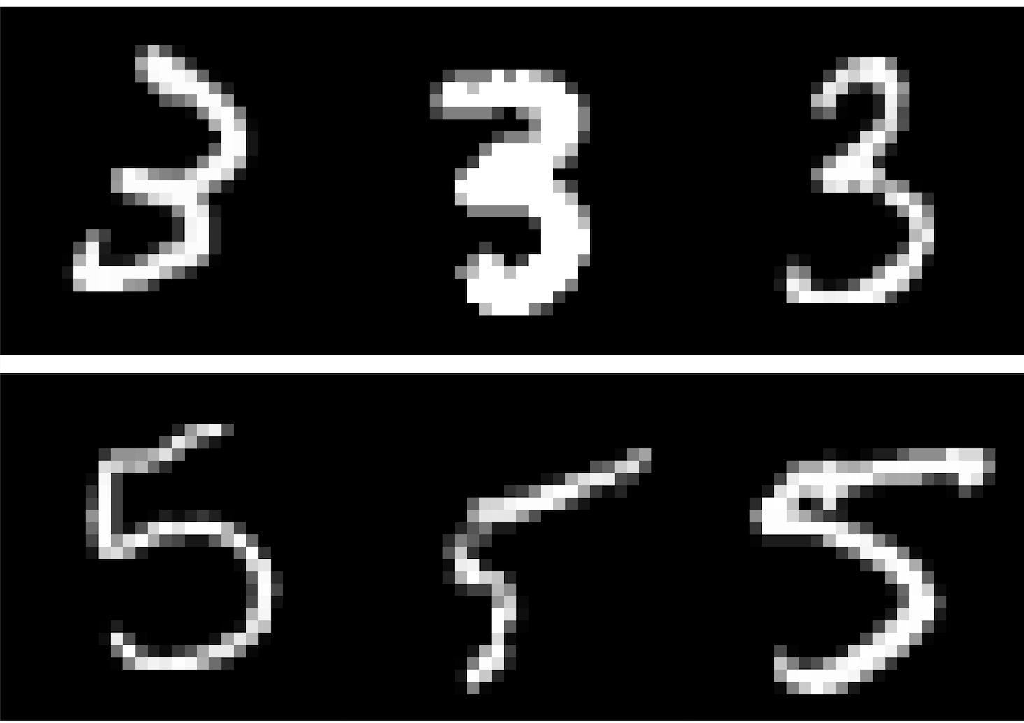
Figure 4: Some samples of 3s and 5s in the MNIST dataset.

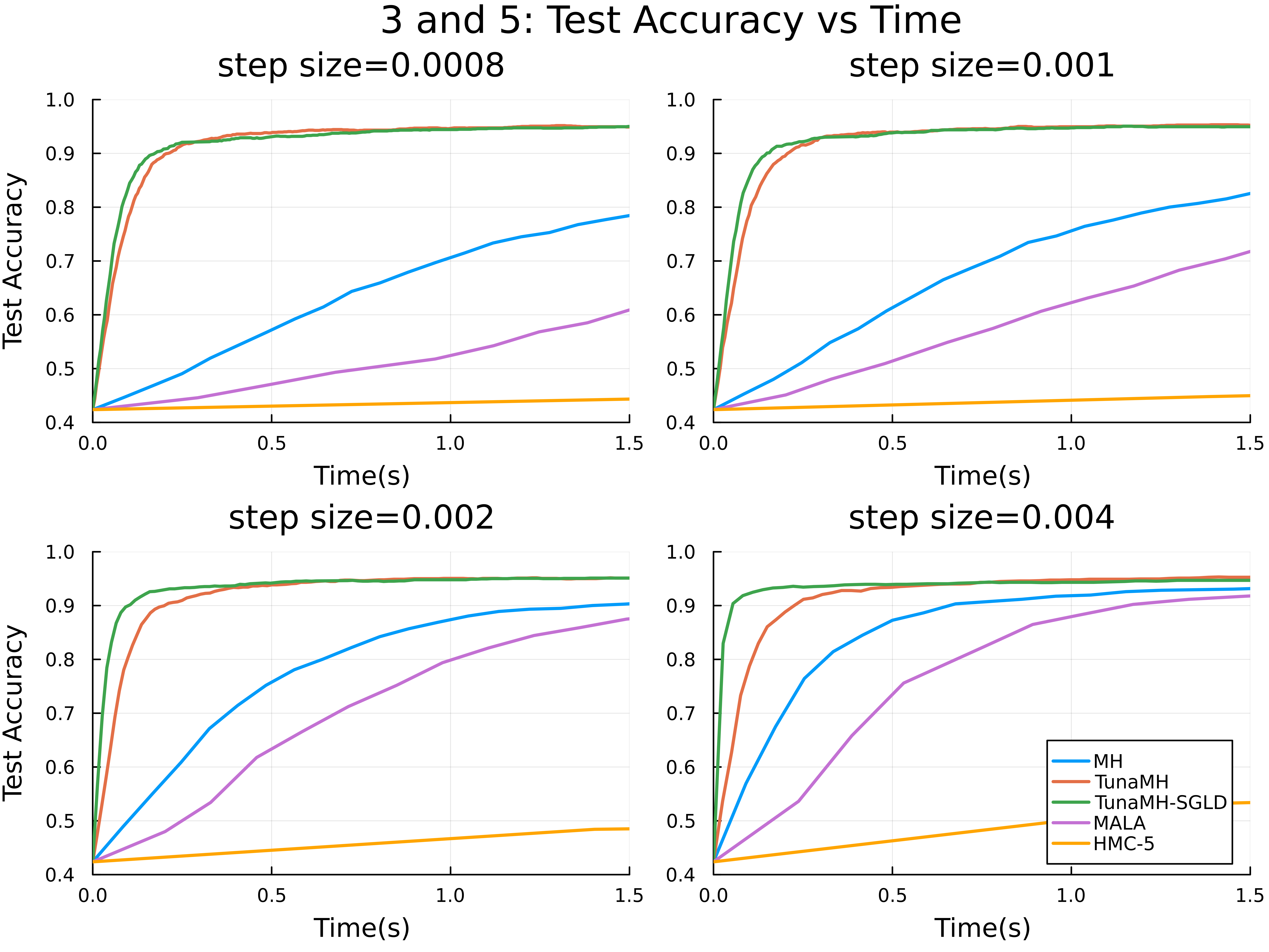
Figure 5: Test accuracy as a function of time.

For TunaMH and TunaMH–SGLD, we follow Zhang et al., (2020) and set the hyperparameter $\chi=10^{-5}$. The batch size $\lvert B\rvert$ in TunaMH–SGLD is set as $20$, so the computation overhead is minimal. We also clip the gradient norm to 2. The original study tests step sizes of $0.0008$ for TunaMH and $0.004$ for random-walk Metropolis. Therefore, we choose step sizes $\{0.0008,0.001,0.002,0.004\}$ for all algorithms. HMC uses 5 leapfrog steps. More extensive comparisons are provided in the supplementary.

The test accuracy comparisons are shown in Figure 5. Due to an extra minibatch for gradient estimation, TunaMH–SGLD converges faster than TunaMH for all step sizes, especially larger ones. Both of them significantly outperform full batch methods, consistent with our previous observations. HMC converges poorly with the stepsizes considered.

Supplementary E.3 includes more extensive experiments, testing all algorithms with larger step sizes and comparing their performance when optimally tuned. Supplementary E.4 compares these algorithms using Bayesian logistic regression for classifying 7s and 9s.

6 Future directions

Our framework opens new avenues for algorithm development. For minibatch MCMC algorithms, future research should extend beyond i.i.d. data. With the i.i.d. assumption, the cost per iteration scales linearly with the minibatch size, so a minibatch with 5% of the data costs roughly 5% of the full batch per step. However, for non-i.i.d. models, evaluating the full-posterior often scales quadratically or cubically with the sample size. Thus, evaluating a minibatch with 5% of the data may cost only 0.25% or less compared to full batch methods. This makes designing minibatch MCMC algorithms for non-i.i.d. cases, such as spatial models and independent component analysis, more urgent.

Another intriguing question is the source of performance gains in minibatch MCMC algorithms. Empirically, these algorithms often achieve ESS/s values 10-100 times greater than MCMC algorithms running on the entire dataset. However, it is proven in Johndrow et al., (2020) that several minibatch algorithms, including Maclaurin and Adams, (2014), but not those considered here, do not significantly improve performance for realistic problems like generalised linear models. Understanding this discrepancy may relate to the concept of “coresets,” as discussed in Huggins et al., (2016); Campbell and Broderick, (2018, 2019).

Appendix A Additional proofs

A.1 Proof of Proposition 1

Proof of Proposition 1.

For unbiasedness, integrating both sides of (1) with respect to $\omega$ gives:

$$\pi(\theta\mid x)\mathbb{E}_{P_{\theta\rightarrow\theta^{\prime}}}[R_{\theta\rightarrow\theta^{\prime}}(\omega)]=\pi(\theta^{\prime}\mid x)\int P_{\theta^{\prime}\rightarrow\theta}(\omega)\mathrm{d}\omega=\pi(\theta^{\prime}\mid x),$$

where the second equality follows from the fact that integrating a probability measure over the entire space equals one. Dividing both sides by $\pi(\theta\mid x)$ gives us the desired result.

For reversibility, we prove this by checking the detailed balance equation. For every fixed $\theta\neq\theta^{\prime}$, we aim to show:

$$\pi(\theta\mid x)K(\theta,\theta^{\prime}) =\pi(\theta^{\prime}\mid x)K(\theta^{\prime},\theta)$$

Expanding the left side of the above equation:

$$\pi(\theta\mid x)K(\theta,\theta^{\prime}) =\pi(\theta\mid x)q(\theta,\theta^{\prime})\mathbb{E}_{\omega}\left[\min\left(R_{\theta\rightarrow\theta^{\prime}}(\omega)\frac{q(\theta^{\prime},\theta)}{q(\theta,\theta^{\prime})},1\right)\right]$$

$$=\int_{\Omega}\pi(\theta\mid x)q(\theta,\theta^{\prime})P_{\theta\rightarrow\theta^{\prime}}(\omega)\min\left(R_{\theta\rightarrow\theta^{\prime}}(\omega)\frac{q(\theta^{\prime},\theta)}{q(\theta,\theta^{\prime})},1\right)\mathrm{d}\omega$$

$$=\int_{\Omega}\min\left(\pi(\theta\mid x)P_{\theta\rightarrow\theta^{\prime}}(\omega)R_{\theta\rightarrow\theta^{\prime}}(\omega)q(\theta^{\prime},\theta),\pi(\theta\mid x)q(\theta,\theta^{\prime})P_{\theta\rightarrow\theta^{\prime}}(\omega)\right)\mathrm{d}\omega$$

$$=\int_{\Omega}\min\left(\pi(\theta^{\prime}\mid x)P_{\theta^{\prime}\rightarrow\theta}(\omega)q(\theta^{\prime},\theta),\pi(\theta\mid x)q(\theta,\theta^{\prime})P_{\theta\rightarrow\theta^{\prime}}(\omega)\right)\mathrm{d}\omega\qquad\qquad\quad~{}~{}\text{by \eqref{eqn:detailed-balance-one-auxiliary}}$$

$$=\int_{\Omega}\min\left(\pi(\theta^{\prime}\mid x)P_{\theta^{\prime}\rightarrow\theta}(\omega)q(\theta^{\prime},\theta),q(\theta,\theta^{\prime})R_{\theta^{\prime}\rightarrow\theta}(\omega)\pi(\theta^{\prime}\mid x)P_{\theta^{\prime}\rightarrow\theta}(\omega)\right)\mathrm{d}\omega\qquad\text{by \eqref{eqn:detailed-balance-one-auxiliary}}$$

$$=\int_{\Omega}\pi(\theta^{\prime}\mid x)P_{\theta^{\prime}\rightarrow\theta}(\omega)q(\theta^{\prime},\theta)\min\left(1,\frac{q(\theta,\theta^{\prime})}{q(\theta^{\prime},\theta)}R_{\theta^{\prime}\rightarrow\theta}(\omega)\right)\mathrm{d}\omega$$

$$=\pi(\theta^{\prime}\mid x)q(\theta^{\prime},\theta)\mathbb{E}_{\omega}\left[\min\left(1,\frac{q(\theta,\theta^{\prime})}{q(\theta^{\prime},\theta)}R_{\theta^{\prime}\rightarrow\theta}(\omega)\right)\right]$$

$$=\pi(\theta^{\prime}\mid x)K(\theta^{\prime},\theta),$$

gives the desired result. ∎

A.2 Verification of examples in Section 2

A.2.1 Verification of Example 1

To check equation (1), recall $\pi(x):=\int\pi(\theta)p_{\theta}(x)\mathrm{d}\theta$ is the marginal distribution of $x$:

$$R_{\theta\rightarrow\theta^{\prime}}(\omega)\cdot\pi(\theta\mid x)\cdot P_{\theta\rightarrow\theta^{\prime}}(\omega) =\frac{\pi(\theta^{\prime})f_{\theta^{\prime}}(x)f_{\theta}(\omega)}{\pi(\theta)f_{\theta}(x)f_{\theta^{\prime}}(\omega)}\cdot\frac{\pi(\theta)f_{\theta}(x)}{Z(\theta)\pi(x)}\cdot\frac{f_{\theta^{\prime}}(\omega)}{Z(\theta^{\prime})}$$

$$=\frac{\pi(\theta^{\prime})f_{\theta^{\prime}}(x)f_{\theta}(\omega)}{\cancel{\pi(\theta)f_{\theta}(x)}\cancel{f_{\theta^{\prime}}(\omega)}}\cdot\frac{\cancel{\pi(\theta)f_{\theta}(x)}}{Z(\theta)\pi(x)}\cdot\frac{\cancel{f_{\theta^{\prime}}(\omega)}}{Z(\theta^{\prime})}$$

$$=\frac{\pi(\theta^{\prime})f_{\theta^{\prime}}(x)}{\pi(x)Z(\theta^{\prime})}\cdot\frac{f_{\theta}(\omega)}{Z(\theta)}$$

$$=\pi(\theta^{\prime}\mid x)p_{\theta}(\omega)$$

$$=\pi(\theta^{\prime}\mid x)P_{\theta^{\prime}\rightarrow\theta}(\omega).$$

All the equalities follow from either the Bayes formula, or the problem definition.

A.2.2 Verification of Example 2

To check equation (1), recall $\pi(\theta\mid x)=\exp(\sum_{i=1}^{N}\phi_{i}(\theta;x))/Z(x)$ :

$$R_{\theta\rightarrow\theta^{\prime}}(\omega)\cdot\pi(\theta\mid x)\cdot P_{\theta\rightarrow\theta^{\prime}}(\omega)=R_{\theta\rightarrow\theta^{\prime}}(\omega)\frac{\exp(\sum_{i=1}^{N}\phi_{i}(\theta;x))}{Z(x)}\prod_{i=1}^{N}P_{\theta\rightarrow\theta^{\prime}}(s_{i})$$

$$=\frac{1}{Z(x)}\prod_{i=1}^{N}\left(\frac{\lambda M_{i}L^{-1}+\phi_{i}(\theta^{\prime};x)}{\lambda M_{i}L^{-1}+\phi_{i}(\theta;x)}\right)^{s_{i}}\cdot e^{\phi_{i}(\theta;x)}\cdot e^{-\lambda M_{i}L^{-1}}e^{-\phi_{i}(\theta;x)}\frac{\left(\lambda M_{i}L^{-1}+\phi_{i}(\theta;x)\right)^{s_{i}}}{s_{i}!}$$

$$=\frac{1}{Z(x)}\prod_{i=1}^{N}\left(\frac{\lambda M_{i}L^{-1}+\phi_{i}(\theta^{\prime};x)}{\cancel{\lambda M_{i}L^{-1}+\phi_{i}(\theta;x)}}\right)^{s_{i}}\cdot\cancel{e^{\phi_{i}(\theta;x)}}\cdot e^{-\lambda M_{i}L^{-1}}\cancel{e^{-\phi_{i}(\theta;x)}}\frac{\left(\cancel{\lambda M_{i}L^{-1}+\phi_{i}(\theta;x)}\right)^{s_{i}}}{s_{i}!}$$

$$=\frac{1}{Z(x)}\prod_{i=1}^{N}\frac{\left(\lambda M_{i}L^{-1}+\phi_{i}(\theta^{\prime};x)\right)^{s_{i}}}{s_{i}!}(e^{-\lambda M_{i}L^{-1}}e^{-\phi_{i}(\theta^{\prime};x)})e^{\phi_{i}(\theta^{\prime};x)}$$

$$=\pi(\theta^{\prime}\mid x)\prod_{i=1}^{N}P_{\theta^{\prime}\rightarrow\theta}(s_{i})$$

$$=\pi(\theta^{\prime}\mid x)P_{\theta^{\prime}\rightarrow\theta}(\omega).$$

A.2.3 Verification of Example 3

To verify equation (1), first recall $\pi(\theta\mid x)=\exp\left(-\sum_{i=1}^{N}U_{i}(\theta;x)\right)/Z(x)$, and the definition

$$\phi_{i}(\theta,\theta^{\prime};x)=\frac{U_{i}(\theta^{\prime};x)-U_{i}(\theta;x)}{2}+\frac{c_{i}}{2}M(\theta,\theta^{\prime}).$$

It is useful to observe:

$$U_{i}(\theta;x)+\phi(\theta,\theta^{\prime};x)=\frac{U_{i}(\theta^{\prime};x)+U_{i}(\theta;x)}{2}+\frac{c_{i}M(\theta,\theta^{\prime})}{2}=U_{i}(\theta^{\prime};x)+\phi(\theta^{\prime},\theta;x).$$

We have :

$$R_{\theta\rightarrow\theta^{\prime}}(\omega)\cdot\pi(\theta\mid x)\cdot P_{\theta\rightarrow\theta^{\prime}}(\omega)=R_{\theta\rightarrow\theta^{\prime}}(\omega)\frac{\exp\left(-\sum_{i=1}^{N}U_{i}(\theta;x)\right)}{Z(x)}\prod_{i=1}^{N}P_{\theta\rightarrow\theta^{\prime}}(s_{i})$$

$$=\frac{1}{Z(x)}\prod_{i=1}^{N}\left(\frac{\lambda c_{i}C^{-1}+\phi_{i}(\theta^{\prime},\theta;x)}{\lambda c_{i}C^{-1}+\phi_{i}(\theta,\theta^{\prime};x)}\right)^{s_{i}}\cdot e^{-\phi_{i}(\theta,\theta^{\prime};x)}\cdot e^{-\lambda c_{i}C^{-1}}e^{-U_{i}(\theta;x)}\frac{\left(\lambda c_{i}C^{-1}+\phi_{i}(\theta,\theta^{\prime};x)\right)^{s_{i}}}{s_{i}!}$$

$$=\frac{1}{Z(x)}\prod_{i=1}^{N}\left(\frac{\lambda c_{i}C^{-1}+\phi_{i}(\theta^{\prime},\theta;x)}{\cancel{\lambda c_{i}C^{-1}+\phi_{i}(\theta,\theta^{\prime};x)}}\right)^{s_{i}}\cdot e^{-\phi_{i}(\theta^{\prime},\theta;x)}\cdot e^{-\lambda c_{i}C^{-1}}e^{-U_{i}(\theta^{\prime};x)}\frac{\left(\cancel{\lambda M_{i}L^{-1}+\phi_{i}(\theta;x)}\right)^{s_{i}}}{s_{i}!}$$

$$=\frac{1}{Z(x)}\prod_{i=1}^{N}\frac{\left(\lambda c_{i}C^{-1}+\phi_{i}(\theta^{\prime},\theta;x)\right)^{s_{i}}}{s_{i}!}(e^{-\lambda c_{i}C^{-1}}e^{-\phi_{i}(\theta^{\prime},\theta;x)})e^{-U_{i}(\theta^{\prime};x)}$$

$$=\pi(\theta^{\prime}\mid x)\prod_{i=1}^{N}P_{\theta^{\prime}\rightarrow\theta}(s_{i})$$

$$=\pi(\theta^{\prime}\mid x)P_{\theta^{\prime}\rightarrow\theta}(\omega).$$

A.3 Proof of Proposition 2

Proof of Proposition 2.

For each $\theta\in\Theta$, the probability distribution $\mathbb{P}_{\mathsf{aux}}(\theta,\cdot)$ can be decomposed as a point-mass at $\theta$ and a density on $\Theta$, namely:

$$\mathbb{P}_{\mathsf{aux}}(\theta,\mathrm{d}\theta^{\prime})=R(\theta)\delta_{\theta}(\mathrm{d}\theta^{\prime})+p_{\mathsf{aux}}(\theta,\theta^{\prime})\lambda(\mathrm{d}\theta^{\prime}),$$

where $\lambda$ is the base measure on $\Theta$ defined earlier. Our goal is to show $\pi(\theta)p_{\mathsf{aux}}(\theta,\theta^{\prime})=\pi(\theta^{\prime})p_{\mathsf{aux}}(\theta^{\prime},\theta)$ for every pair $(\theta,\theta^{\prime})$ satisfying $\theta\neq\theta^{\prime}$. Reversibility will directly result from this equality. The term $p_{\mathsf{aux}}(\theta,\theta^{\prime})$ describes the density of successfully moving from $\theta$ to $\theta^{\prime}$, including two steps: proposing $\theta^{\prime}$ and then accepting the transition. Therefore we have the following expression of $p_{\mathsf{aux}}(\theta,\theta^{\prime})$:

$$p_{\mathsf{aux}}(\theta,\theta^{\prime})=$$

$$\int_{\Omega_{1}}\mathbb{P}_{\theta}(\omega_{1})q_{\omega_{1}}(\theta,\theta^{\prime})\int_{\Omega_{2}}\left(\min\left\{1,\frac{\Pi(\theta^{\prime})\mathbb{P}_{\theta^{\prime},\theta}(\omega_{1},\omega_{2})}{\Pi(\theta)\mathbb{P}_{\theta,\theta^{\prime}}(\omega_{1},\omega_{2})}\cdot\frac{q_{w_{1}}(\theta^{\prime},\theta)}{q_{w_{1}}(\theta,\theta^{\prime})}\right\}\mathbb{P}_{\theta,\theta^{\prime}}(\omega_{2}\mid\omega_{1})\lambda_{2}(\mathrm{d}\omega_{2})\right)\lambda_{1}(\mathrm{d}\omega_{1}).$$

Therefore we have

$$\Pi(\theta) p_{\mathsf{aux}}(\theta,\theta^{\prime})=$$

$$\int\min\bigg{\{}\Pi(\theta)\mathbb{P}_{\theta,\theta^{\prime}}(\omega_{1},\omega_{2})q_{\omega_{1}}(\theta,\theta^{\prime}),\Pi(\theta^{\prime})\mathbb{P}_{\theta^{\prime},\theta}(\omega_{1},\omega_{2})q_{w_{1}}(\theta^{\prime},\theta)\bigg{\}}\lambda_{1}\otimes\lambda_{2}(\mathrm{d}\omega_{1}\mathrm{d}\omega_{2}),$$

which is symmetric over $\theta$ and $\theta^{\prime}$. This shows $\Pi(\theta)p_{\mathsf{aux}}(\theta,\theta^{\prime})=\Pi(\theta^{\prime})p_{\mathsf{aux}}(\theta^{\prime},\theta).$ ∎

A.4 Algorithmic description of the idealised chain

Algorithm 7 idealised MH

1:  Initialise: Initial state $\theta_{0}$; number of iterations $T$; target distribution $\pi(\theta\mid x)$

2:  for $t=0$ to $T-1$ do

3:     propose $\theta^{\prime}\sim Q_{\mathsf{ideal}}(\theta,\cdot)$

4:     compute the acceptance ratio

$$r\xleftarrow{}\frac{\pi(\theta^{\prime}\mid x)}{\pi(\theta_{t}\mid x)}\cdot\frac{q_{\mathsf{ideal}}(\theta^{\prime},\theta_{t})}{q_{\mathsf{ideal}}(\theta_{t},\theta^{\prime})}$$

5:     with probability $\min\{1,r\}$, set $\theta_{t+1}\xleftarrow{}\theta^{\prime}$; otherwise, $\theta_{t+1}\xleftarrow{}\theta_{t}$

6:  end for

A.5 Proof of Lemma 1

Proof of Lemma 1.

We write $p_{\mathsf{aux}}(\theta,\theta^{\prime})$ in its integral form, and upper bound it as follows:

$$p_{\mathsf{aux}}(\theta,\theta^{\prime}) =\int_{\Omega_{1}\times\Omega_{2}}\mathbb{P}_{\theta}(\omega_{1})q_{\omega_{1}}(\theta,\theta^{\prime})\mathbb{P}_{\theta,\theta^{\prime}}(\omega_{2}\mid\omega_{1})r(\theta,\theta^{\prime};\omega_{1},\omega_{2})\lambda_{1}\otimes\lambda_{2}(\mathrm{d}\omega_{1}\mathrm{d}\omega_{2})$$

$$=\int_{\Omega_{1}}\mathbb{P}_{\theta}(\omega_{1})q_{\omega_{1}}(\theta,\theta^{\prime})\left(\mathbb{E}_{\omega_{2}\mid\omega_{1},\theta,\theta^{\prime}}\left[\min\left\{\frac{\pi(\theta^{\prime}\mid x)\mathbb{P}_{\theta^{\prime},\theta}(\omega_{1},\omega_{2})}{\pi(\theta\mid x)\mathbb{P}_{\theta,\theta^{\prime}}(\omega_{1},\omega_{2})}\cdot\frac{q_{w_{1}}(\theta^{\prime},\theta)}{q_{w_{1}}(\theta,\theta^{\prime})},1\right\}\right]\right)\lambda_{1}(\mathrm{d}\omega_{1})$$

$$\leq\int_{\Omega_{1}}\mathbb{P}_{\theta}(\omega_{1})q_{\omega_{1}}(\theta,\theta^{\prime})\left(\min\left\{\frac{\pi(\theta^{\prime}\mid x)q_{w_{1}}(\theta^{\prime},\theta)}{\pi(\theta\mid x)q_{w_{1}}(\theta,\theta^{\prime})}\mathbb{E}_{\omega_{2}\mid\omega_{1},\theta,\theta^{\prime}}\left[\frac{\mathbb{P}_{\theta^{\prime},\theta}(\omega_{1},\omega_{2})}{\mathbb{P}_{\theta,\theta^{\prime}}(\omega_{1},\omega_{2})}\right],1\right\}\right)\lambda_{1}(\mathrm{d}\omega_{1})$$

$$=\int_{\Omega_{1}}\mathbb{P}_{\theta}(\omega_{1})q_{\omega_{1}}(\theta,\theta^{\prime})\left(\min\left\{\frac{\pi(\theta^{\prime}\mid x)q_{w_{1}}(\theta^{\prime},\theta)}{\pi(\theta\mid x)q_{w_{1}}(\theta,\theta^{\prime})}\frac{\mathbb{P}_{\theta^{\prime}}(\omega_{1})}{\mathbb{P}_{\theta}(\omega_{1})},1\right\}\right)\lambda_{1}(\mathrm{d}\omega_{1})$$

$$=p_{\mathsf{MwG}}(\theta,\theta^{\prime})$$

The first inequality follows from $\mathbb{E}[\min\{ah(X),c\}]\leq\min\{a\mathbb{E}[h(X)],c\}$, treating $\omega_{2}$ as a random variable, and using the fact that

$$\mathbb{E}_{\omega_{2}\mid\omega_{1},\theta,\theta^{\prime}}\left[\frac{\mathbb{P}_{\theta^{\prime},\theta}(\omega_{1},\omega_{2})}{\mathbb{P}_{\theta,\theta^{\prime}}(\omega_{1},\omega_{2})}\right] =\int_{\Omega_{2}}\frac{\mathbb{P}_{\theta^{\prime}}(\omega_{1})\mathbb{P}_{\theta^{\prime},\theta}(\omega_{2}\mid\omega_{1})}{\mathbb{P}_{\theta}(\omega_{1})\mathbb{P}_{\theta,\theta^{\prime}}(\omega_{2}\mid\omega_{1})}\mathbb{P}_{\theta,\theta^{\prime}}(\omega_{2}\mid\omega_{1})\lambda_{2}(\mathrm{d}\omega_{2})$$

$$=\frac{\mathbb{P}_{\theta^{\prime}}(\omega_{1})}{\mathbb{P}_{\theta}(\omega_{1})}.$$

The last equality follows from the calculations in Case 2.

Furthermore

$$p_{\mathsf{MwG}}(\theta,\theta^{\prime}) \leq\min\left\{\int\frac{\pi(\theta^{\prime}\mid x)}{\pi(\theta\mid x)}q_{w_{1}}(\theta^{\prime},\theta)\mathbb{P}_{\theta^{\prime}}(\omega_{1})\lambda_{1}(\mathrm{d}\omega_{1}),\int q_{\omega_{1}}(\theta,\theta^{\prime})\mathbb{P}_{\theta}(\omega_{1})\lambda_{1}(\mathrm{d}\omega_{1})\right\}$$

$$=\min\left\{\frac{\pi(\theta^{\prime}\mid x)}{\pi(\theta\mid x)}q_{\mathsf{ideal}}(\theta^{\prime},\theta),q_{\mathsf{ideal}}(\theta,\theta^{\prime})\right\}$$

$$=q_{\mathsf{ideal}}(\theta,\theta^{\prime})\min\left\{\frac{\pi(\theta^{\prime}\mid x)}{\pi(\theta\mid x)}\frac{q_{\mathsf{ideal}}(\theta^{\prime},\theta)}{q_{\mathsf{ideal}}(\theta,\theta^{\prime})},1\right\}$$

$$=p_{\mathsf{ideal}}(\theta,\theta^{\prime}).$$

Here, the inequality uses the fact $\int\min\{f,g\}\leq\min\{\int f,\int g\}$. ∎

A.6 Proof of Theorem 1

Proof of Theorem 1.

We can write down the transition density as:

$$p_{\mathsf{aux}}(\theta,\theta^{\prime}) =\int_{\Omega_{1}\times\Omega_{2}}\mathbb{P}_{\theta}(\omega_{1})q_{\omega_{1}}(\theta,\theta^{\prime})\mathbb{P}_{\theta,\theta^{\prime}}(\omega_{2}\mid\omega_{1})r(\theta,\theta^{\prime};\omega_{1},\omega_{2})\lambda_{1}\otimes\lambda_{2}(\mathrm{d}\omega_{1}\mathrm{d}\omega_{2})$$

$$=\int_{\Omega_{1}}\mathbb{P}_{\theta}(\omega_{1})q_{\omega_{1}}(\theta,\theta^{\prime})\left(\mathbb{E}_{\omega_{2}\mid\omega_{1},\theta,\theta^{\prime}}\left[\min\left\{\frac{\pi(\theta^{\prime}\mid x)\mathbb{P}_{\theta^{\prime},\theta}(\omega_{1},\omega_{2})}{\pi(\theta\mid x)\mathbb{P}_{\theta,\theta^{\prime}}(\omega_{1},\omega_{2})}\cdot\frac{q_{w_{1}}(\theta^{\prime},\theta)}{q_{w_{1}}(\theta,\theta^{\prime})},1\right\}\right]\right)\lambda_{1}(\mathrm{d}\omega_{1})$$

$$\geq\int_{\Omega_{1}}\mathbb{P}_{\theta}(\omega_{1})q_{\omega_{1}}(\theta,\theta^{\prime})\left(\min\left\{\frac{\pi(\theta^{\prime}\mid x)q_{w_{1}}(\theta^{\prime},\theta)}{\pi(\theta\mid x)q_{w_{1}}(\theta,\theta^{\prime})}\frac{\mathbb{P}_{\theta^{\prime}}(\omega_{1})}{\mathbb{P}_{\theta}(\omega_{1})},1\right\}\right)$$

$$\qquad\times\left(\int_{\Omega_{2}}\min\left\{\mathbb{P}_{\theta,\theta^{\prime}}(\omega_{2}\mid\omega_{1}),\mathbb{P}_{\theta^{\prime},\theta}(\omega_{2}\mid\omega_{1})\right\}\lambda_{2}(\mathrm{d}\omega_{2})\right)\lambda_{1}(\mathrm{d}\omega_{1})$$

$$=\int_{\Omega_{1}}\mathbb{P}_{\theta}(\omega_{1})q_{\omega_{1}}(\theta,\theta^{\prime})\left(\min\left\{\frac{\pi(\theta^{\prime}\mid x)q_{w_{1}}(\theta^{\prime},\theta)}{\pi(\theta\mid x)q_{w_{1}}(\theta,\theta^{\prime})}\frac{\mathbb{P}_{\theta^{\prime}}(\omega_{1})}{\mathbb{P}_{\theta}(\omega_{1})},1\right\}\right)$$

$$\qquad\times\left(1-d_{\sf TV}(\theta,\theta^{\prime},\omega_{1})\right)\lambda_{1}(\mathrm{d}\omega_{1})$$

$$\geq\left(1-d_{\sf TV}(\theta,\theta^{\prime})\right)\int_{\Omega_{1}}\mathbb{P}_{\theta}(\omega_{1})q_{\omega_{1}}(\theta,\theta^{\prime})\left(\min\left\{\frac{\pi(\theta^{\prime}\mid x)q_{w_{1}}(\theta^{\prime},\theta)}{\pi(\theta\mid x)q_{w_{1}}(\theta,\theta^{\prime})}\frac{\mathbb{P}_{\theta^{\prime}}(\omega_{1})}{\mathbb{P}_{\theta}(\omega_{1})},1\right\}\right)$$

$$=\left(1-d_{\sf TV}(\theta,\theta^{\prime})\right)p_{\mathsf{MwG}}(\theta,\theta^{\prime}).$$

The first inequality follows from the fact $\min\{ab,cd\}\geq\min\{a,c\}\min\{b,d\}$ for $a,b,c,d\geq 0$. For the second inequality in the statement of Theorem 1, first recall the improved version of Bretagnolle–Huber inequality in Section 8.3 of Gerchinovitz et al., (2020), which states:

$$1-d_{\sf TV}(P,Q)\geq e^{-1/e}\exp\{-d_{\sf KL}(P||Q)\}.$$

The original Bretagnolle–Huber inequality Bretagnolle and Huber, (1979); Canonne, (2022) is a slightly weaker version where the constant $e^{-1/e}$ is replaced by $1/2$. Replacing $P,Q$ by $\mathbb{P}_{\theta,\theta^{\prime}}(\omega_{2}\mid\omega_{1}),\mathbb{P}_{\theta^{\prime},\theta}(\omega_{2}\mid\omega_{1})$, and taking the supremum (for $d_{\sf TV}$) over $\omega_{1}$, we get:

$$p_{\mathsf{aux}}(\theta,\theta^{\prime}) \geq e^{-1/e}\exp\{\tilde{d}_{\sf KL}(\theta,\theta^{\prime})\}\}p_{\mathsf{MwG}}(\theta,\theta^{\prime}).$$

Meanwhile, reversing the order between $P,Q$ in the Bretagnolle–Huber inequality, we have

$$1-d_{\sf TV}(Q,P)\geq e^{-1/e}\exp\{-d_{\sf KL}(Q||P)\}.$$

This implies

$$p_{\mathsf{aux}}(\theta,\theta^{\prime}) \geq e^{-1/e}\exp\{\tilde{d}_{\sf KL}(\theta^{\prime},\theta)\}\}p_{\mathsf{MwG}}(\theta,\theta^{\prime}).$$

Finally, multiplying the improved Bretagnolle–Huber inequality for $(P,Q)$ and $(Q,P)$ together and then taking the square root, we obtain:

$$1-d_{\sf TV}(P,Q)\geq e^{-1/e}\exp\{-0.5(d_{\sf KL}(P||Q)+d_{\sf KL}(Q||P))\},$$

which further shows

$$1-d_{\sf TV}(\theta,\theta^{\prime})\geq e^{-1/e}\exp\{-d_{\sf KL}(\theta,\theta^{\prime})\}.$$

This concludes the proof of Theorem 1. ∎

A.7 Proof of Theorem 2

It is useful to recall the defintion of the Dirichlet form. The Dirichlet form of a function $f$ with respect to Markov transition kernel $P$ is ${\mathcal{E}}(P,f):=\lVert(I-P)f,f\rVert_{\Pi}=0.5\int\int(f(x)-f(y))^{2}\Pi(\mathrm{d}x)P(x,\mathrm{d}y).$ When $P$ is reversible, then ${\mathsf{Gap}}(P)=\inf_{f\in L^{2}_{0}(\Pi),f\neq 0}{\mathcal{E}}(P,f)/\lVert f\rVert_{\Pi}^{2}$.

Proof of Theorem 2.

It follows from Theorem 1 that for any $f$, the Dirichlet form satisfies

$${\mathcal{E}}(\mathbb{P}_{\mathsf{aux}},f) \geq\int\int\left(1-d_{\sf TV}(\theta,\theta^{\prime})\right)(f(\theta)-f(\theta^{\prime}))^{2}\mathbb{P}_{\mathsf{MwG}}(\theta,\mathrm{d}\theta^{\prime})\pi(\mathrm{d}\theta\mid x)$$

$$\geq\left(1-\sup_{\theta,\theta^{\prime}}d_{\sf TV}(\theta,\theta^{\prime})\right){\mathcal{E}}(\mathbb{P}_{\mathsf{MwG}},f).$$

Dividing both sides by $\lVert f\rVert_{\Pi}^{2}$ and then taking the infimum over $f\in L^{2}_{0}(\pi(\theta\mid x))$, we have

$${\mathsf{Gap}}(\mathbb{P}_{\mathsf{aux}})\geq(1-\sup_{\theta,\theta^{\prime}}d_{\sf TV}(\theta,\theta^{\prime})){\mathsf{Gap}}(\mathbb{P}_{\mathsf{MwG}}).$$

Similarly, we have

$${\mathcal{E}}(\mathbb{P}_{\mathsf{aux}},f)\geq e^{-1/e}\exp\{-\min\{d_{\sf KL}(\theta,\theta^{\prime}),\tilde{d}_{\sf KL}(\theta,\theta^{\prime}),\tilde{d}_{\sf KL}(\theta^{\prime},\theta)\}{\mathcal{E}}(\mathbb{P}_{\mathsf{MwG}},f).$$

Therefore ${\mathsf{Gap}}(\mathbb{P}_{\mathsf{aux}})\geq\left(e^{-1/e}\exp\{-\min\{d_{\sf KL}(\theta,\theta^{\prime}),\tilde{d}_{\sf KL}(\theta,\theta^{\prime}),\tilde{d}_{\sf KL}(\theta^{\prime},\theta)\}\}\right){\mathsf{Gap}}(\mathbb{P}_{\mathsf{MwG}}).$ ∎

A.8 Proof of Proposition 4

Proof of Proposition 4.

Our first result is derived directly by recognizing that $\mathbb{P}_{\theta,\theta^{\prime}}$ within our general framework corresponds to $p_{\theta^{\prime}}$ in the exchange algorithm. The second result follows from the observation:

$$1-d_{\sf TV}(p_{\theta},p_{\theta^{\prime}})=\mathbb{E}_{p_{\theta^{\prime}}}\left[\min\{1,\frac{p_{\theta}}{p_{\theta^{\prime}}}\}\right]\geq\delta\mathbb{P}_{p_{\theta^{\prime}}}(A_{\theta,\theta^{\prime}}(\delta))=\epsilon\delta.$$

∎

A.9 Proof of Proposition 5

It is useful to recall a few facts, which we provide proofs for completeness in supplementary A.11: for univariate Poisson random variables with parameter $\lambda_{1},\lambda_{2}$, their KL divergence equals $d_{\sf KL}(\mathsf{Poi}(\lambda_{1})||\mathsf{Poi}(\lambda_{2}))=\lambda_{1}\log(\lambda_{1}/\lambda_{2})+\lambda_{2}-\lambda_{1}$. Meanwhile, the KL divergence $d_{\sf KL}(\mathsf{Poi}(\lambda_{1})||\mathsf{Poi}(\lambda_{2}))$ satisfying $m\leq\lambda_{1}\leq\lambda_{2}\leq M$ is maximised when $\lambda_{1}=m$ and $\lambda_{2}=M$. Furthermore, KL divergence satisfies the ‘tensorization property’, i.e., $d_{\sf KL}(\otimes_{i}P_{i}||\otimes_{i}Q_{i})=\sum_{i}d_{\sf KL}(P_{i}||Q_{i})$, while $1-d_{\sf TV}(\otimes_{i}P_{i},\otimes_{i}Q_{i})\geq\prod_{i}(1-d_{\sf TV}(P_{i},Q_{i}))$.

Proof of Proposition 5.

Let $\tilde{\lambda}_{i}(\theta):=\lambda M_{i}/L+\phi_{i}(\theta;x)$. We recognise that $\mathbb{P}_{\theta,\theta^{\prime}}=\otimes_{i=1}^{N}\mathsf{Poi}(\tilde{\lambda}_{i}(\theta))$ in PoissonMH. We have $1-d_{\sf TV}(\mathbb{P}_{\theta,\theta^{\prime}},\mathbb{P}_{\theta^{\prime},\theta})\geq\prod_{i}\left(1-d_{\sf TV}(\mathsf{Poi}(\tilde{\lambda}_{i}(\theta)),\mathsf{Poi}(\tilde{\lambda}_{i}(\theta^{\prime})))\right).$ For each term in the product, assuming without loss of generality that $\tilde{\lambda}_{i}(\theta^{\prime})>\tilde{\lambda}_{i}(\theta)$:

$$1-d_{\sf TV}(\mathsf{Poi}(\tilde{\lambda}_{i}(\theta)),\mathsf{Poi}(\tilde{\lambda}_{i}(\theta^{\prime}))) \geq e^{-1/e}\exp\left\{-d_{\sf KL}\left(\mathsf{Poi}(\tilde{\lambda}_{i}(\theta))||\mathsf{Poi}(\tilde{\lambda}_{i}(\theta^{\prime}))\right)\right\}.$$

The KL divergence satisfies:

$$d_{\sf KL}\left(\mathsf{Poi}(\tilde{\lambda}_{i}(\theta))||\mathsf{Poi}(\tilde{\lambda}_{i}(\theta^{\prime}))\right) \leq\tilde{\lambda}_{i}(\theta)\log\left(\tilde{\lambda}_{i}(\theta)/\tilde{\lambda}_{i}(\theta^{\prime})\right)+\tilde{\lambda}_{i}(\theta^{\prime})-\tilde{\lambda}_{i}(\theta)$$

$$\leq(\lambda M_{i}/L)\frac{-M_{i}}{\lambda M_{i}/L+M_{i}}+M_{i}=\frac{LM_{i}}{\lambda+L}.$$

Here the second inequality uses the fact $\tilde{\lambda}_{i}(\theta)\in[\lambda M_{i}/L,\lambda M_{i}/L+M_{i}]$ for every $\theta$. Putting these together shows

$$1- d_{\sf TV}(\mathbb{P}_{\theta,\theta^{\prime}},\mathbb{P}_{\theta^{\prime},\theta})\geq e^{-1/e}\exp\left\{-\sum_{i}\frac{LM_{i}}{\lambda+L}\right\}=e^{-1/e}\exp\left\{-\frac{L^{2}}{\lambda+L}\right\}.$$

Thus ${\mathsf{Gap}}(\mathbb{P}_{\mathsf{aux}})\geq e^{-1/e}\exp\left\{-\frac{L^{2}}{\lambda+L}\right\}{\mathsf{Gap}}(\mathbb{P}_{\mathsf{ideal}})$.

We can also use the second part of Theorem 2, and calculate the symmetrised KL:

$$d_{\sf KL}(\mathbb{P}_{\theta,\theta^{\prime}}||\mathbb{P}_{\theta^{\prime},\theta})+d_{\sf KL}(\mathbb{P}_{\theta^{\prime},\theta}||\mathbb{P}_{\theta,\theta^{\prime}})$$

$$=\sum_{i=1}^{N}\left(\tilde{\lambda}_{i}(\theta)\log\frac{\tilde{\lambda}_{i}(\theta)}{\tilde{\lambda}_{i}(\theta^{\prime})}+\cancel{\tilde{\lambda}_{i}(\theta^{\prime})-\tilde{\lambda}_{i}(\theta)}\right)+\sum_{i=1}^{N}\left(\tilde{\lambda}_{i}(\theta^{\prime})\log\frac{\tilde{\lambda}_{i}(\theta^{\prime})}{\tilde{\lambda}_{i}(\theta)}+\cancel{\tilde{\lambda}_{i}(\theta)-\tilde{\lambda}_{i}(\theta^{\prime})}\right)$$

$$\leq\log\left(1+\frac{L}{\lambda}\right)\sum_{i=1}^{N}\lvert\tilde{\lambda}_{i}(\theta^{\prime})-\tilde{\lambda}_{i}(\theta)\rvert\leq\log\left(1+\frac{L}{\lambda}\right)\sum_{i=1}^{N}M_{i}=L\log\left(1+\frac{L}{\lambda}\right).$$

Therefore, applying Theorem 2, we get:

$${\mathsf{Gap}}(\mathbb{P}_{\mathsf{aux}})\geq e^{-1/e}\left(1+\frac{L}{\lambda}\right)^{-L/2}{\mathsf{Gap}}(\mathbb{P}_{\mathsf{ideal}})\geq e^{-1/e}\exp\left\{\frac{-L^{2}}{2\lambda}\right\}{\mathsf{Gap}}(\mathbb{P}_{\mathsf{ideal}}).$$

∎

A.10 Proof of Proposition 6

Proof of Proposition 6.

Let $\tilde{\phi}_{i}(\theta,\theta^{\prime}):=\lambda c_{i}/C+\phi_{i}(\theta,\theta^{\prime};x)$. We have $\mathbb{P}_{\theta,\theta^{\prime}}=\otimes_{i=1}^{N}\mathsf{Poi}(\tilde{\phi}_{i}(\theta,\theta^{\prime}))$ for TunaMH. We can calculate the symmetrised KL divergence

$$d_{\sf KL}(\mathbb{P}_{\theta,\theta^{\prime}}||\mathbb{P}_{\theta^{\prime},\theta})+d_{\sf KL}(\mathbb{P}_{\theta^{\prime},\theta}||\mathbb{P}_{\theta,\theta^{\prime}})$$

$$=\sum_{i=1}^{N}\left(\tilde{\phi}_{i}(\theta,\theta^{\prime})\log\frac{\tilde{\phi}_{i}(\theta,\theta^{\prime})}{\tilde{\phi}_{i}(\theta^{\prime},\theta)}+\cancel{\tilde{\phi}_{i}(\theta^{\prime},\theta)-\tilde{\phi}_{i}(\theta,\theta^{\prime})}\right)+\sum_{i=1}^{N}\left(\tilde{\phi}_{i}(\theta^{\prime},\theta)\log\frac{\tilde{\phi}_{i}(\theta^{\prime},\theta)}{\tilde{\phi}_{i}(\theta,\theta^{\prime})}+\cancel{\tilde{\phi}_{i}(\theta,\theta^{\prime})-\tilde{\phi}_{i}(\theta^{\prime},\theta)}\right)$$

$$=\sum_{i=1}^{N}\left(\log\left(\tilde{\phi}_{i}(\theta,\theta^{\prime})/\tilde{\phi}_{i}(\theta^{\prime},\theta)\right)\right)\left(\tilde{\phi}_{i}(\theta,\theta^{\prime})-\tilde{\phi}_{i}(\theta^{\prime},\theta)\right)$$

$$\leq\sum_{i=1}^{N}c_{i}M(\theta,\theta^{\prime})\log\left(\frac{\lambda c_{i}/C+c_{i}M}{\lambda c_{i}/C}\right)$$

$$\leq\sum_{i=1}^{N}c_{i}M(\theta,\theta^{\prime})\frac{CM(\theta,\theta^{\prime})}{\lambda}=\frac{C^{2}M^{2}(\theta,\theta^{\prime})}{\chi C^{2}M^{2}(\theta,\theta^{\prime})}=\frac{1}{\chi}.$$

Therefore, applying Theorem 2, we get:

$${\mathsf{Gap}}(\mathbb{P}_{\mathsf{aux}})\geq e^{-1/e}\exp\{-\frac{1}{2\chi}\}{\mathsf{Gap}}(\mathbb{P}_{\mathsf{ideal}}).$$

∎

A.11 Proof of auxiliary results

Here we prove several auxiliary results mentioned in Section 4.4. Even though many of these results are well-known, we include proofs here for clarity and completeness.

Proposition 7.

For univariate Poisson random variables with parameter $\lambda_{1},\lambda_{2}$, their KL divergence equals $d_{\sf KL}(\mathsf{Poi}(\lambda_{1})||\mathsf{Poi}(\lambda_{2}))=\lambda_{1}\log(\lambda_{1}/\lambda_{2})+\lambda_{2}-\lambda_{1}$.

Proof of Proposition 7.

Let

$$P_{\lambda}(n):=\exp\{-\lambda\}\frac{\lambda^{n}}{n!}$$

be the probability mass function of a $\mathsf{Poi}(\lambda)$ random variable evaluating at $n\in\mathbb{N}$. By definition, we have:

$$d_{\sf KL}(\mathsf{Poi}(\lambda_{1})||\mathsf{Poi}(\lambda_{2}))=\mathbb{E}_{X\sim\mathsf{Poi}(\lambda_{1})}\left[\log\left(\frac{P_{\lambda_{1}}(X)}{P_{\lambda_{2}}(X)}\right)\right].$$

Therefore,

$$d_{\sf KL}(\mathsf{Poi}(\lambda_{1})||\mathsf{Poi}(\lambda_{2})) =\mathbb{E}_{X\sim\mathsf{Poi}(\lambda_{1})}\left[-\lambda_{1}+\lambda_{2}+X\log\left(\frac{\lambda_{1}}{\lambda_{2}}\right)\right]$$

$$=\lambda_{2}-\lambda_{1}+\log\left(\frac{\lambda_{1}}{\lambda_{2}}\right)\mathbb{E}_{X\sim\mathsf{Poi}(\lambda_{1})}[X]$$

$$=\lambda_{1}\log\left(\frac{\lambda_{1}}{\lambda_{2}}\right)+\lambda_{2}-\lambda_{1}.$$

∎

Proposition 8.

For any $\lambda_{1},\lambda_{2}$ satisfying $0\leq m\leq\lambda_{1}\leq\lambda_{2}\leq M$, we have

$$d_{\sf KL}(\mathsf{Poi}(\lambda_{1})||\mathsf{Poi}(\lambda_{2}))\leq d_{\sf KL}(\mathsf{Poi}(m)||\mathsf{Poi}(M)).$$

Proof of Proposition 8.

The proposition is equivalent to proving that the function $g(\lambda_{1},\lambda_{2}):=\lambda_{1}\log(\lambda_{1}/\lambda_{2})+\lambda_{2}-\lambda_{1}$, constrained within the region $m\leq\lambda_{1}\leq\lambda_{2}\leq M$, is maximised at $\lambda_{1}=m$ and $\lambda_{2}=M$. We first fix $\lambda_{1},$ and take derivative with respect to $\lambda_{2}$:

$$\partial_{\lambda_{2}}g(\lambda_{1},\lambda_{2})=-\frac{\lambda_{1}}{\lambda_{2}}+1.$$

The derivative is non-negative as $\lambda_{2}\geq\lambda_{1}$. Therefore, $g(\lambda_{1},\lambda_{2})\leq g(\lambda_{1},M)$. Then we arbitrarily fix $\lambda_{2}$, and take derivative with respect to $\lambda_{1}$:

$$\partial_{\lambda_{1}}g(\lambda_{1},\lambda_{2})=\log(\lambda_{1})+1-\log(\lambda_{2})-1=\log(\lambda_{1})-\log(\lambda_{2})\leq 0.$$

Therefore, $g(\lambda_{1},\lambda_{2})\leq g(m,\lambda_{2})$. Putting these two inequalities together, we know:

$$d_{\sf KL}(\mathsf{Poi}(\lambda_{1})||\mathsf{Poi}(\lambda_{2}))=g(\lambda_{1},\lambda_{2})\leq g(m,M)=d_{\sf KL}(\mathsf{Poi}(m)||\mathsf{Poi}(M)).$$

∎

Proposition 9.

Let $P_{i},Q_{i}$ be two probability measures on the same measurable space $(\Omega_{i},{\mathcal{F}}_{i})$ for $i\in\{1,2,\ldots,M\}$. Then we have

$$d_{\sf KL}(\otimes_{i=1}^{M}P_{i}||\otimes_{i}Q_{i})=\sum_{i=1}^{M}d_{\sf KL}(P_{i}||Q_{i})$$

and

$$1-d_{\sf TV}(\otimes_{i=1}^{M}P_{i},\otimes_{i}Q_{i})\geq\prod_{i=1}^{M}(1-d_{\sf TV}(P_{i},Q_{i})).$$

Proof.

Let $P:=\otimes_{i=1}^{M}P_{i}$ and $Q:=\otimes_{i=1}^{M}Q_{i}$, and $X=(X_{1},\ldots,X_{M})\sim P$. Then

$$d_{\sf KL}(P||Q) =\mathbb{E}_{X\sim P}\left[\log\left(\frac{P(X)}{Q(X)}\right)\right]$$

$$=\mathbb{E}_{X\sim P}\left[\sum_{i=1}^{M}\log\left(\frac{P(X_{i})}{Q(X_{i})}\right)\right]$$

$$=\sum_{i=1}^{M}\mathbb{E}_{X_{i}\sim P_{i}}\left[\log\left(\frac{P(X_{i})}{Q(X_{i})}\right)\right]$$

$$=\sum_{i=1}^{M}d_{\sf KL}(P_{i}||Q_{i}),$$

which proves the first equality.

For the second equality, recall the fact $d_{\sf TV}(\mu,\nu)=1-\sup_{(X,Y)\in\Gamma(\mu,\nu)}\mathbb{P}(X=Y)$. Here, $\Gamma(\mu,\nu)$ denotes all the couplings of $\mu$ and $\nu$ (that is, all the joint distributions with the marginal distributions $\mu$ and $\nu$). Now fix any $\epsilon>0$, for each $i\in\{1,\ldots,M\}$, choose $\Pi_{i}\in\Gamma(P_{i},Q_{i})$ such that

$$\mathbb{P}_{(X_{i},Y_{i})\sim\Pi_{i}}(X=Y)\geq 1-d_{{\sf TV}}(P_{i},Q_{i})-\epsilon.$$

Consider the $2M$-dimensional vector $(X_{1},Y_{1},X_{2},Y_{2},\ldots,X_{M},Y_{M})\sim\prod_{i=1}^{M}\Pi_{i}$, then the joint distribution of $X=(X_{1},\ldots,X_{M})$ and $Y=(Y_{1},\ldots,Y_{M})$ belongs to the $\Gamma(P,Q)$. Hence

$$1-d_{\sf TV}(P,Q)\geq\mathbb{P}(X=Y)=\prod_{i=1}^{n}\mathbb{P}(X_{i}=Y_{i})\geq\prod_{i=1}^{n}(1-d_{{\sf TV}}(P_{i},Q_{i})-\epsilon).$$

Since $\epsilon$ is an arbitrary positive constant, we can let $\epsilon\rightarrow 0$ and get

$$1-d_{\sf TV}(\otimes_{i=1}^{M}P_{i},\otimes_{i}Q_{i})\geq\prod_{i=1}^{M}(1-d_{\sf TV}(P_{i},Q_{i})).$$

∎

A.12 Additional properties

Proposition 10.

Let $a:[0,\infty)\rightarrow[0,1]$ be any fixed function satisfying $a(t)=ta(1/t)$. Let $\tilde{\mathbb{P}}_{\mathsf{aux}}(\cdot,\cdot)$ denote the transition kernel of the Markov chain as defined in Algorithm 4, with the exception that Step 7 is modified to: “with probability $a(r)$, set $\theta_{t+1}\leftarrow\theta^{\prime}$; otherwise, set $\theta_{t+1}\leftarrow\theta_{t}$”. Then $\tilde{\mathbb{P}}_{\mathsf{aux}}(\cdot,\cdot)$ remains reversible with respect to $\pi(\theta\mid x)$.

Proof of Proposition 10.

Let $\tilde{p}_{\mathsf{aux}}$ denote the density part of $\tilde{P}_{\mathsf{aux}}$. We have the following expression of $\tilde{p}_{\mathsf{aux}}(\theta,\theta^{\prime})$:

$$\tilde{p}_{\mathsf{aux}}(\theta,\theta^{\prime})$$

$$=\int_{\Omega_{1}}\mathbb{P}_{\theta}(\omega_{1})q_{\omega_{1}}(\theta,\theta^{\prime})\int_{\Omega_{2}}\left(a\left(\frac{\Pi(\theta^{\prime})\mathbb{P}_{\theta^{\prime},\theta}(\omega_{1},\omega_{2})}{\Pi(\theta)\mathbb{P}_{\theta,\theta^{\prime}}(\omega_{1},\omega_{2})}\cdot\frac{q_{w_{1}}(\theta^{\prime},\theta)}{q_{w_{1}}(\theta,\theta^{\prime})}\right)\mathbb{P}_{\theta,\theta^{\prime}}(\omega_{2}\mid\omega_{1})\lambda_{2}(\mathrm{d}\omega_{2})\right)\lambda_{1}(\mathrm{d}\omega_{1})$$

$$=\frac{\Pi(\theta^{\prime})}{\Pi(\theta)}\int_{\Omega_{1}}\int_{\Omega_{2}}\mathbb{P}_{\theta^{\prime},\theta}(\omega_{1},\omega_{2})q_{\omega_{1}}(\theta^{\prime},\theta)a\left(\frac{\Pi(\theta)\mathbb{P}_{\theta,\theta^{\prime}}(\omega_{1},\omega_{2})}{\Pi(\theta^{\prime})\mathbb{P}_{\theta^{\prime},\theta}(\omega_{1},\omega_{2})}\cdot\frac{q_{w_{1}}(\theta,\theta^{\prime})}{q_{w_{1}}(\theta^{\prime},\theta)}\right)\lambda_{2}(\mathrm{d}\omega_{2})\lambda_{1}(\mathrm{d}\omega_{1})$$

$$=\frac{\Pi(\theta^{\prime})}{\Pi(\theta)}\tilde{p}_{\mathsf{aux}}(\theta^{\prime},\theta),$$

where the second equality uses $a(r)=ra(1/r)$. Therefore we have

$$\Pi(\theta)\tilde{p}_{\mathsf{aux}}(\theta,\theta^{\prime})=\Pi(\theta^{\prime})\tilde{p}_{\mathsf{aux}}(\theta^{\prime},\theta),$$

as desired. ∎

Appendix B Implementation details of locally balanced PoissonMH

According to Livingstone and Zanella, (2022), there are two different implementation versions of the locally balanced proposal on $\mathbb{R}^{d}$. The first approach is to treat each dimension of the parameter space separately. We define the proposal for dimension $j$ as:

$$q_{\omega_{1},j}^{(g)}(\theta,\theta^{\prime}_{j}):=Z^{-1}(\theta,\omega_{1})g\left(e^{\partial_{\theta_{j}}\log\left(\pi(\theta\mid x)\mathbb{P}_{\theta}(\omega_{1})\right)(\theta^{\prime}_{j}-\theta_{j})}\right)\mu_{j}(\theta^{\prime}_{j}-\theta_{j}),$$

where $\mu_{j}$ is a univariate symmetric density. The proposal on $\mathbb{R}^{d}$ is then defined as the product of proposals on each dimension:

$$q_{\omega_{1}}^{(g)}(\theta,\theta^{\prime})=\prod_{j=1}^{d}q_{\omega_{1},j}^{(g)}(\theta,\theta^{\prime}_{j})$$

The second approach is to derive a multivariate version of the locally balanced proposal. Proposition 3.3 and the experiments in Livingstone and Zanella, (2022) show that the first approach is more efficient. As a result, we develop the auxiliary version of the first approach for both Poisson–Barker and Poisson–MALA.

Now, we provide implementation details of Poisson–MALA and Poisson–Barker. First, by taking $g(t)=\sqrt{t}$ and $\mu_{j}\sim\mathbb{N}(0,\sigma^{2})$ for every $j$, we derive the Poisson–MALA proposal as:

$$q_{\omega_{1}}^{M}(\theta,\theta^{\prime})=\prod_{j=1}^{d}q_{\omega_{1},j}^{M}(\theta,\theta^{\prime}_{j}).$$

The $j$-th term in the product can be further represented as

$$q_{\omega_{1},j}^{M}(\theta,\theta^{\prime}_{j}) \propto\exp\left\{\frac{1}{2}\partial_{\theta_{j}}\log\left(\pi(\theta\mid x)\mathbb{P}_{\theta}(\omega_{1})\right)(\theta^{\prime}-\theta_{j})\right\}\exp\left\{-\frac{1}{2\sigma^{2}}(\theta^{\prime}-\ \theta_{j})^{2}\right\}$$

$$\propto\exp\left\{-\frac{1}{2\sigma^{2}}\left(\theta^{\prime}-\theta_{j}-\frac{\sigma^{2}}{2}\partial_{\theta_{j}}\log\left(\pi(\theta\mid x)\mathbb{P}_{\theta}(\omega_{1})\right)\right)^{2}\right\}$$

which is Gaussian centred at $\theta_{j}+\frac{\sigma^{2}}{2}\partial_{\theta_{j}}\log\left(\pi(\theta\mid x)\mathbb{P}_{\theta}(\omega_{1})\right)$ with standard deviation $\sigma$. This proposal is similar to MALA except that we substitute the gradient of $\log\pi(\theta\mid x)$ by the gradient of $\log\pi(\theta\mid x)\mathbb{P}_{\theta}(\omega_{1})$, enabling efficient implementation. Since all the dimensions are independent, our Poisson–MALA proposal is a multivariate Gaussian with mean $\theta+0.5\sigma^{2}\nabla_{\theta}\log\left(\pi(\theta\mid x)\mathbb{P}_{\theta}(\omega_{1})\right)$ and covariance matrix $\sigma^{2}\mathbb{I}_{d}$.

Next, when taking $g(t)=t/(1+t)$, we can similarly write our Poisson–Barker proposal as:

$$q_{\omega_{1}}^{B}(\theta,\theta^{\prime})=\prod_{j=1}^{d}q_{\omega_{1},j}^{B}(\theta,\theta^{\prime}_{j}).$$

The $j$-th term in the product can be further represented as

$$q_{\omega_{1},j}^{B}(\theta,\theta^{\prime}_{j})=Z^{-1}(\theta,\omega_{1})\frac{\mu_{j}(\theta^{\prime}_{j}-\theta)}{1+e^{-\partial_{\theta_{j}}\log\left(\pi(\theta\mid x)\mathbb{P}_{\theta}(\omega_{1})\right)(\theta^{\prime}_{j}-\theta_{j})}}.$$

Now we claim $Z(\theta,\omega_{1})$ is a constant $0.5$. To verify our claim, we first notice that $g(t)=t/(1+t)=1-g(t^{-1})$. Let $C_{\theta,\omega_{1}}:=\partial_{\theta_{j}}\log\left(\pi(\theta\mid x)\mathbb{P}_{\theta}(\omega_{1})\right)$, we can integrate:

$$Z(\theta,\omega_{1}) =\int_{\mathbb{R}}g(\exp\{C_{\theta,\omega_{1}}(\theta^{\prime}_{j}-\theta_{j})\})\mu_{j}(\theta_{j}^{\prime}-\theta_{j})\mathrm{d}\theta^{\prime}_{j}$$

$$=\int_{\mathbb{R}}g(\exp\{C_{\theta,\omega_{1}}t\})\mu_{j}(t)\mathrm{d}t$$

$$=\int_{t>0}g(\exp\{C_{\theta,\omega_{1}}t\})\mu_{j}(t)\mathrm{d}t+\int_{t<0}g(\exp\{C_{\theta,\omega_{1}}t\})\mu_{j}(t)\mathrm{d}t$$

$$=\int_{t>0}g(\exp\{C_{\theta,\omega_{1}}t\})\mu_{j}(t)\mathrm{d}t+\int_{t>0}g(\exp\{-C_{\theta,\omega_{1}}t\})\mu_{j}(t)\mathrm{d}t\quad\text{since~{}}\mu_{j}(t)=\mu_{j}(-t)$$

$$=\int_{t>0}\mu_{j}(t)\mathrm{d}t$$

$$=0.5.$$

The same calculation is used in Livingstone and Zanella, (2022). Therefore our proposal has an explicit form

$$q_{\omega_{1},j}^{B}(\theta,\theta^{\prime}_{j})=2\frac{\mu_{j}(\theta^{\prime}_{j}-\theta_{j})}{1+e^{-\partial_{\theta_{j}}\log\left(\pi(\theta\mid x)\mathbb{P}_{\theta}(\omega_{1})\right)(\theta^{\prime}_{j}-\theta_{j})}}.$$

Sampling from this proposal distribution can be done perfectly by the following simple procedure: given current $\theta_{j}$, one first propose $z\sim\mu_{j}$, then move to $\theta_{j}+z$ with probability $g(e^{\partial_{\theta_{j}}\log\left(\pi(\theta\mid x)\mathbb{P}_{\theta}(\omega_{1})\right)z})$, and to $\theta_{j}-z$ with probability $1-g(e^{\partial_{\theta_{j}}\log\left(\pi(\theta\mid x)\mathbb{P}_{\theta}(\omega_{1})\right)z})$. This procedure samples exactly from $q_{\omega_{1},j}^{B}(\theta,\theta^{\prime}_{j})$, see also Proposition 3.1 of Livingstone and Zanella, (2022) for details. Sampling from the $d$-dimensional proposal can be done by implementing the above strategy for each dimensional independently.

Both algorithms require evaluating $\nabla\log\left(\pi(\theta\mid x)\mathbb{P}_{\theta}(\omega_{1})\right)$, and we verify that this only requires evaluation on the same minibatch as PoissonMH. As derived in Section 3.3.1,

$$\pi(\theta\mid x)\mathbb{P}_{\theta}(\omega_{1}) =\frac{1}{Z(x)}\exp(-\lambda)\prod_{i:s_{i}>0}\frac{\left(\lambda M_{i}L^{-1}+\phi_{i}(\theta;x)\right)^{s_{i}}}{s_{i}!}.$$

Then, we take the logarithm:

$$\log\pi(\theta\mid x)\mathbb{P}_{\theta}(\omega_{1})=-\log Z(x)-\lambda-\sum_{i:s_{i}>0}s_{i}!+\sum_{i:s_{i}>0}s_{i}\log\left\{\lambda M_{i}L^{-1}+\phi_{i}(\theta;x)\right\}.$$

The gradient is:

$$\nabla_{\theta}\log\pi(\theta\mid x)\mathbb{P}_{\theta}(\omega_{1})=\sum_{i:s_{i}>0}s_{i}\frac{\nabla_{\theta}\phi_{i}(\theta;x)}{\lambda M_{i}L^{-1}+\phi_{i}(\theta;x)}$$

As a result, we only need to evaluate the gradient on the minibatch data.

Appendix C Additional comment on Algorithm 2 and 3

A close examination of Algorithm 2 and 3 shows that the key ingredient is the ‘Poisson estimator’, which provides an unbiased estimate of the exponential of an expectation. In the case of tall dataset, the quantity of interest is the target ratio which can be represented as $\exp{\{\sum_{i=1}^{N}(\phi_{i}(\theta^{\prime};x)-\phi_{i}(\theta;x))\}}$ in Algorithm 2 (or $\exp{\{(-\sum_{i=1}^{N}U_{i}(\theta^{\prime};x)+U_{i}(\theta;x))\}}$ in Algorithm 3). This ratio can be evaluated precisely, albeit at a high cost. Alternatively, we can express the ratio as $\exp\left(\mathbb{E}[f(I)]\right)$, where $f(i):=N(\phi_{i}(\theta^{\prime};x)-\phi_{i}(\theta;x))$ and $I\sim\mathsf{Unif}\{1,2,\ldots,N\}$. This formulation aligns the problem with the Poisson estimator’s framework. An additional subtly is the estimator has to be non-negative, as it will be used to determine the acceptance probability (Step 7–8 in Algorithm 2, and Step 8–9 in Algorithm 3). Consequently, all the technical assumptions and design elements in both Algorithm 2 and 3 are intended to ensure that the non-negativity of the Poisson estimator. Other applications of the Poisson estimator can be found in Fearnhead et al., (2010); Wagner, (1987); Papaspiliopoulos, (2011) and the references therein. This insight can be interpreted either positively or negatively: it implies that there is potential for developing new algorithms using similar ideas under weaker assumptions (such as non-i.i.d. data or less stringent technical conditions). However, eliminating all technical assumptions seems unlikely due to the impossibility result in Theorem 2.1 of Jacob and Thiery, (2015).

Appendix D Further details of experiments in Section 5

D.1 Heterogeneous truncated Gaussian

Recall that for fixed $\theta$, our data $\{y_{1},y_{2},\ldots,y_{N}\}$ is assumed to be i.i.d. with distribution $y_{i}\mid\theta\sim\mathbb{N}(\theta,\Sigma)$. With uniform prior on the hypercube $[-K,K]^{d}$, our target is the following tempered posterior:

$$\pi(\theta\mid y) \propto\exp\left\{-\frac{1}{2}\beta\sum_{i=1}^{N}(\theta-y_{i})^{\intercal}\Sigma^{-1}(\theta-y_{i})\right\}\mathbb{I}(\theta\in[-K,K]^{d})$$

Now we look at the function $\tilde{\phi}_{i}(\theta)=-\frac{1}{2}\beta(\theta-y_{i})^{\intercal}\Sigma^{-1}(\theta-y_{i})$. It is clear that $\tilde{\phi}_{i}(\theta)\leq 0$. On the other hand:

$$\tilde{\phi}_{i}(\theta)\geq-\frac{1}{2}\beta\lambda_{\max}(\Sigma^{-1})\lVert\theta-y_{i}\rVert_{2}^{2}\geq-\frac{1}{2}\beta\lambda_{\max}(\Sigma^{-1})\sum_{j=1}^{d}(\lvert y_{ij}\rvert+K)^{2},$$

where $\lambda_{\max}(\Sigma^{-1})$ is the largest eigenvalue of $\Sigma^{-1}$. Set

$$M_{i}:=\frac{1}{2}\beta\lambda_{\max}(\Sigma^{-1})\sum_{j=1}^{d}(\lvert y_{ij}\rvert+K)^{2},$$

and define $\phi_{i}(\theta):=\tilde{\phi}_{i}(\theta)+M_{i}$, we have $\phi_{i}(\theta)\in[0,M_{i}]$ for each $i$. Meanwhile, the posterior is $\pi(\theta\mid y)\propto\exp\{\sum_{i=1}^{N}\phi_{i}(\theta)\}$, as adding a constant to $\tilde{\phi}_{i}(\theta)$ does not affect the posterior.

D.2 Robust Linear Regression

Similarly, we can derive a bound for each

$$\tilde{\phi}_{i}(\theta):=-\frac{v+1}{2}\log\left(1+\frac{(y_{i}-\theta^{\intercal}x_{i})^{2}}{v}\right)$$

in the robust linear regression example. Suppose we constraint $\theta$ in the region$\{\theta,\lVert\theta\rVert_{2}\leq R\}$, then in order to get the upper bound $M_{i}$, we first find the following maximum:

$$\max_{\theta}(y_{i}-\theta^{\intercal}x_{i})^{2}\;\text{ subject to }||\theta||_{2}\leq R$$

The above maximization problem can be solved analytically, with the solution:

$$\theta^{*}=\begin{cases}\frac{-x_{i}}{||x_{i}||_{2}}\cdot R\;\;\;\text{when }y_{i}>0\\ \\ \frac{x_{i}}{||x_{i}||_{2}}\cdot R\;\;\;\text{when }y_{i}<0.\end{cases}$$

The maximum equals $(|y_{i}|+||x_{i}||_{2}\cdot R)^{2}$ for both cases. Taking

$$M_{i}=\frac{v+1}{2}\log\left(1+\frac{(|y_{i}|+||x_{i}||_{2}\cdot R)^{2}}{v}\right),$$

and set $\phi_{i}(\theta):=\tilde{\phi}_{i}(\theta)+M_{i}$, we have $\phi_{i}(\theta)\in[0,M_{i}]$ for each $i$. Meanwhile, the posterior is $\pi(\theta\mid y)\propto\exp\{\sum_{i=1}^{N}\phi_{i}(\theta)\}$.

D.3 Bayesian Logistic Regression on MNIST

For $i=1,2,\cdots,N$, let $x_{i}\in\mathbb{R}^{d}$ be the features and $y_{i}\in\{0,1\}$ be the label. The logistic regression model is $p_{\theta}(y_{i}=1\mid x)=h(x_{i}^{\top}\theta)\}$, where $h(z):=(1+\exp(-z))^{-1}$ is the sigmoid function. We assume the data are i.i.d distributed. With a flat prior, the target posterior distribution is:

$$\pi(\theta\mid y,x)\propto\exp\left\{-\sum_{i=1}^{N}-y_{i}\log h(x_{i}^{\top}\theta)-(1-y_{i})\log h(-x_{i}^{\top}\theta)\right\}.$$

Let us denote $U_{i}(\theta)=-y_{i}\log h(x_{i}^{\top}\theta)-(1-y_{i})\log h(-x_{i}^{\top}\theta)$. To derive the required bound for $U_{i}(\theta)$ in Algorithm 3 and 6, first notice that $U_{i}(\theta)$ is continuous and convex with gradient $\nabla_{\theta}U_{i}(\theta)=(h(x_{i}^{\top}\theta)-y_{i})\cdot x_{i}$. Then, we have:

$$U_{i}(\theta^{\prime})-U_{i}(\theta)\leq\nabla_{\theta}U_{i}(\theta)^{\top}(\theta^{\prime}-\theta)$$

and

$$|U_{i}(\theta^{\prime})-U_{i}(\theta)| \leq\lVert\nabla_{\theta}U_{i}(\theta)\rVert_{2}\cdot\lVert\theta^{\prime}-\theta\rVert_{2}$$

$$\leq\lVert x_{i}\rVert_{2}\cdot\lVert\theta^{\prime}-\theta\rVert_{2}$$

where the first inequality follows from Cauchy–Schwarz inequality and the second inequality comes from $|(h(x_{i}^{\top}\theta)-y_{i})|\leq 1$. Thus, we can take $M_{i}(\theta,\theta^{\prime})=\lVert\theta^{\prime}-\theta\rVert_{2}$ and $c_{i}=\lVert x_{i}\rVert_{2}$ for TunaMH and TunaMH–SGLD.

Appendix E Additional experiments

E.1 Additional experiments on 10-dimensional robust linear regression

Figure 6 compares the MSE over iteration count for all six algorithms in the robust linear regression example. It is clear that random-walk Metropolis outperforms PoissonMH, confirming our theoretical results in Section 4.1. However, PoissonMH has better performance in clock time due to its lower per-step cost. Poisson–MALA and MALA exhibit the best overall per-iteration performance, followed by HMC and Poisson–Barker. This indicates that our locally-balanced PoissonMH method can find proposals as effective as full batch methods while enjoying a very low per-step cost.

Figure 7 compares HMC with 2, 5, and 10 leapfrog steps. Their performances are similar for all acceptance rates, with 10 leapfrog steps being slightly better. Therefore, the HMC used in Section 5.2 uses 10 leapfrog steps.

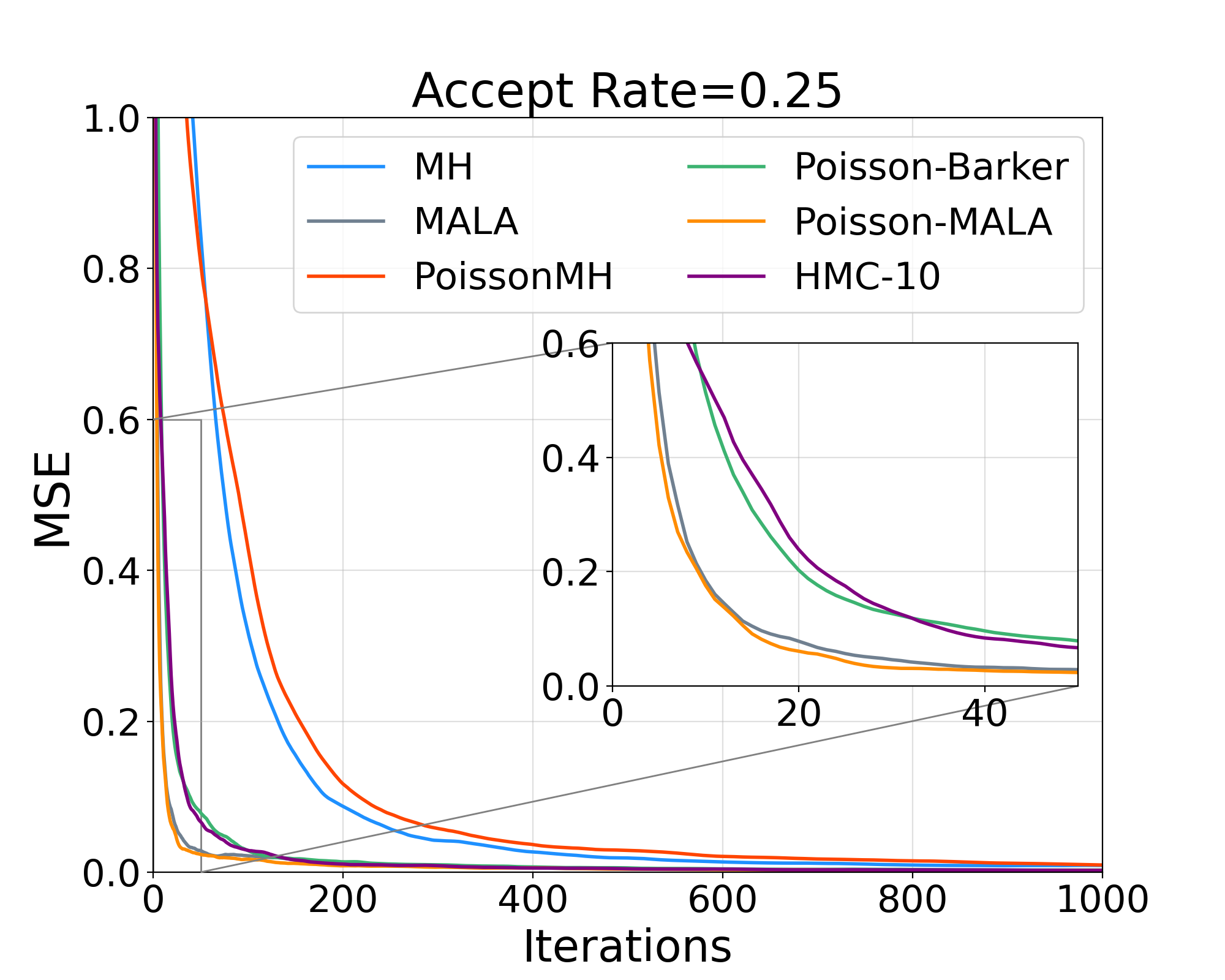
(a) acceptance rate=0.25

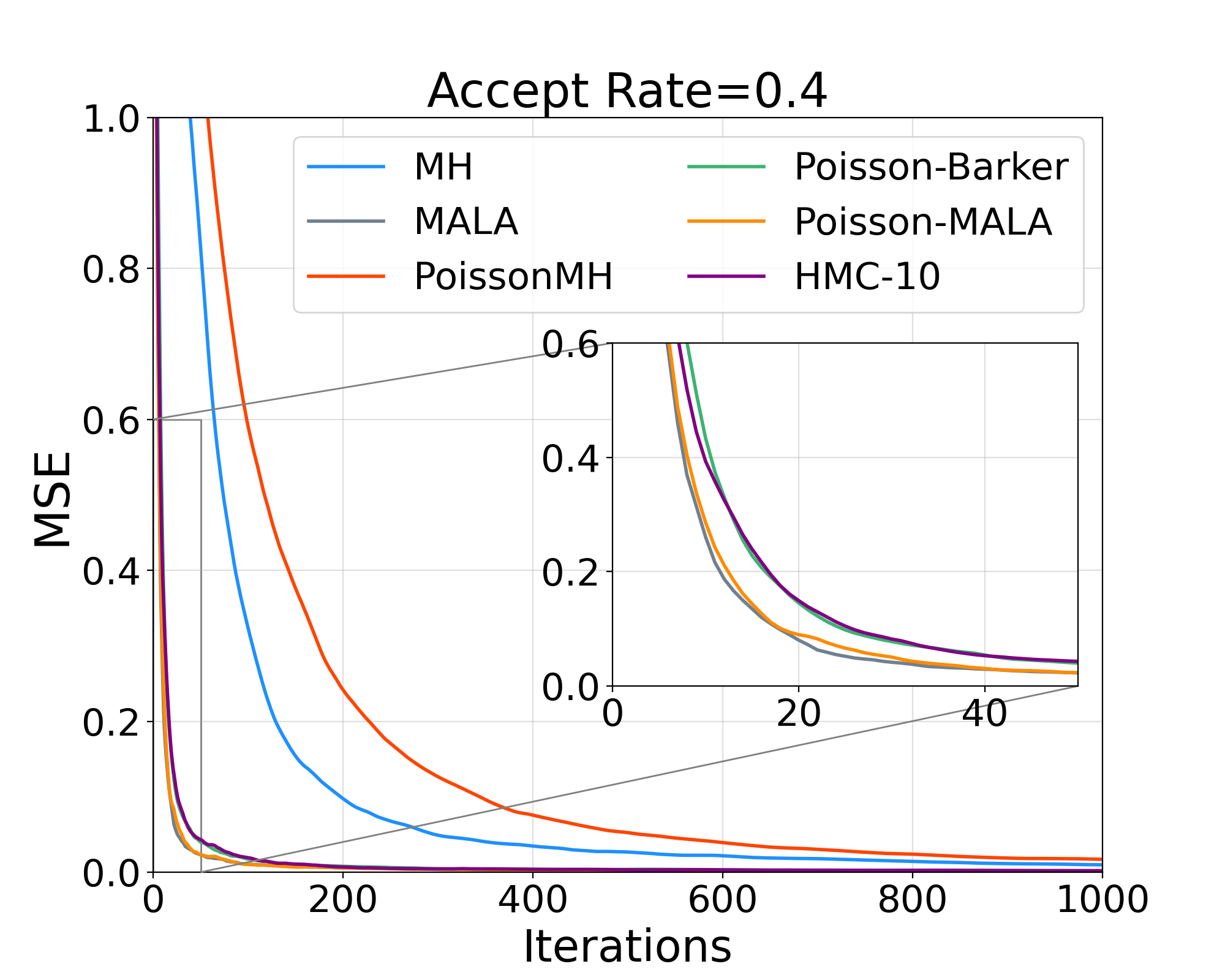
(b) acceptance rate=0.4

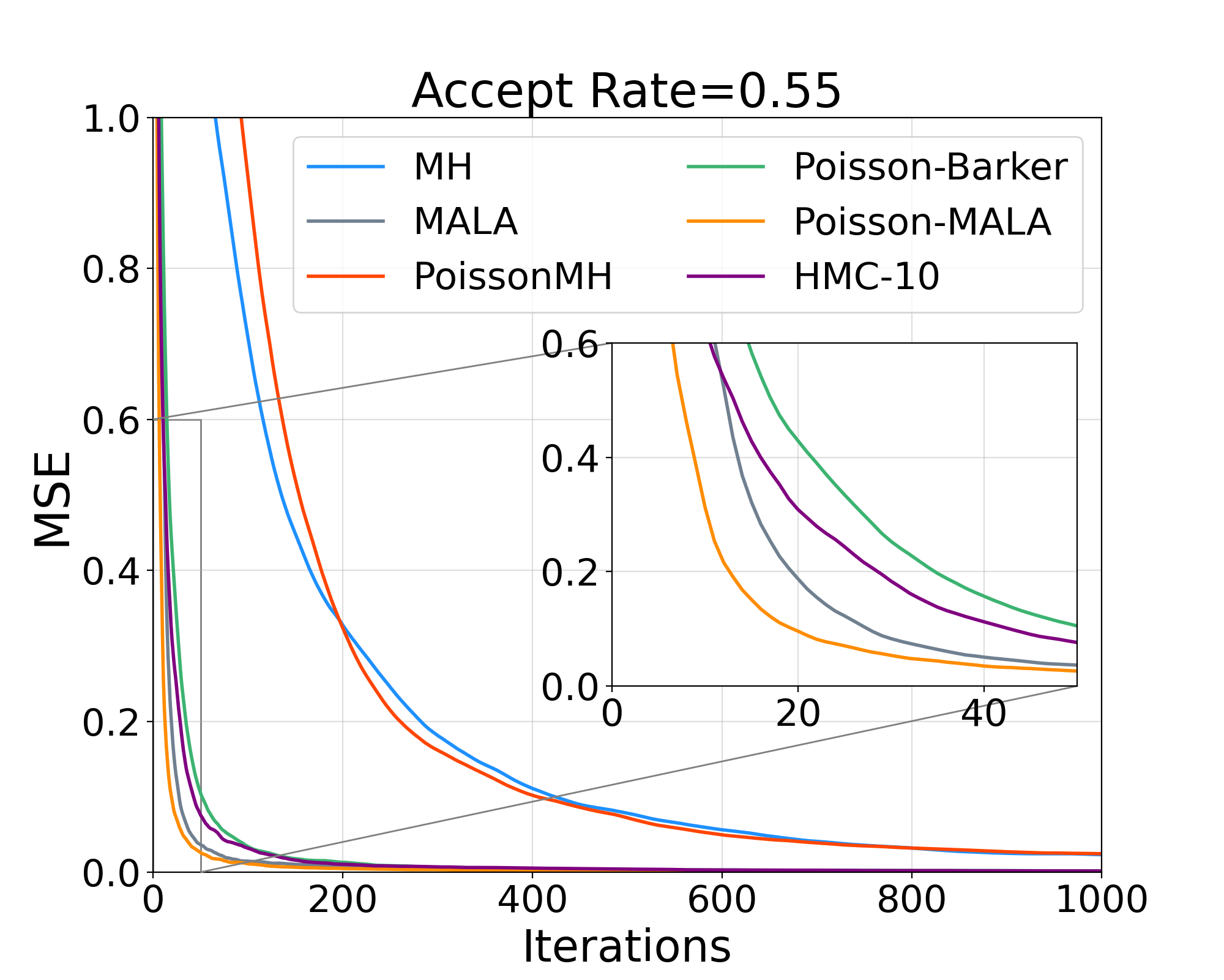
(c) acceptance rate=0.55

Figure 6: Iteration-wise MSE comparison. MSE of $\theta^{\star}$ as a function of iteration count different acceptance rates. The three large plots show the performance of all methods in the first 1000 steps. The three inside plots zoom in on Poisson-Barker, and Poisson-MALA, MALA, and HMC in the first 50 steps. All results are averaged over 10 runs.

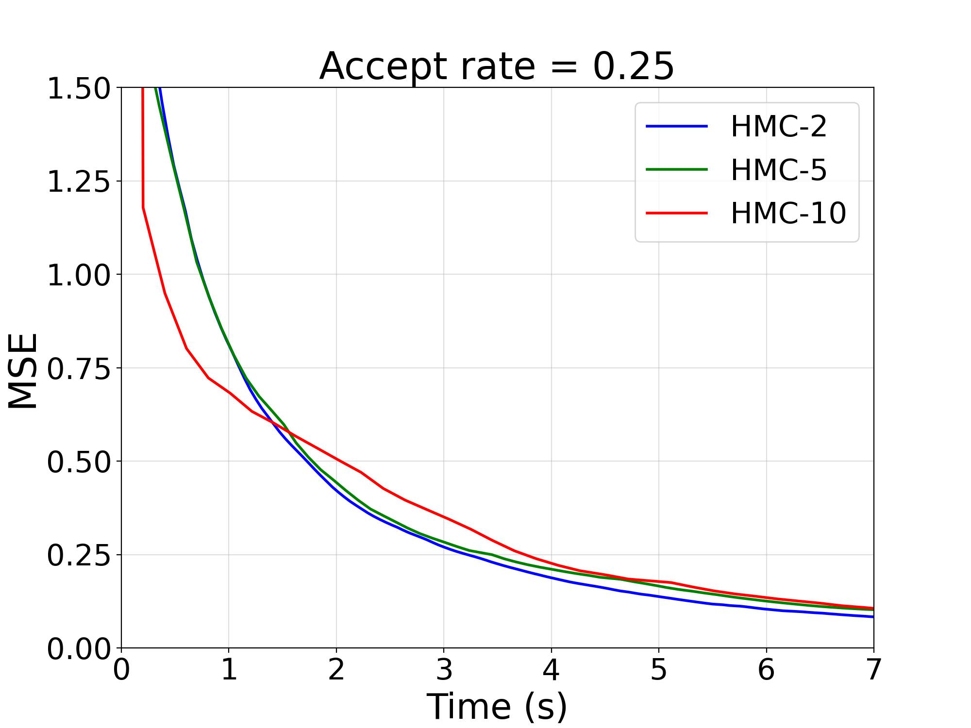
(a) acceptance rate=0.25

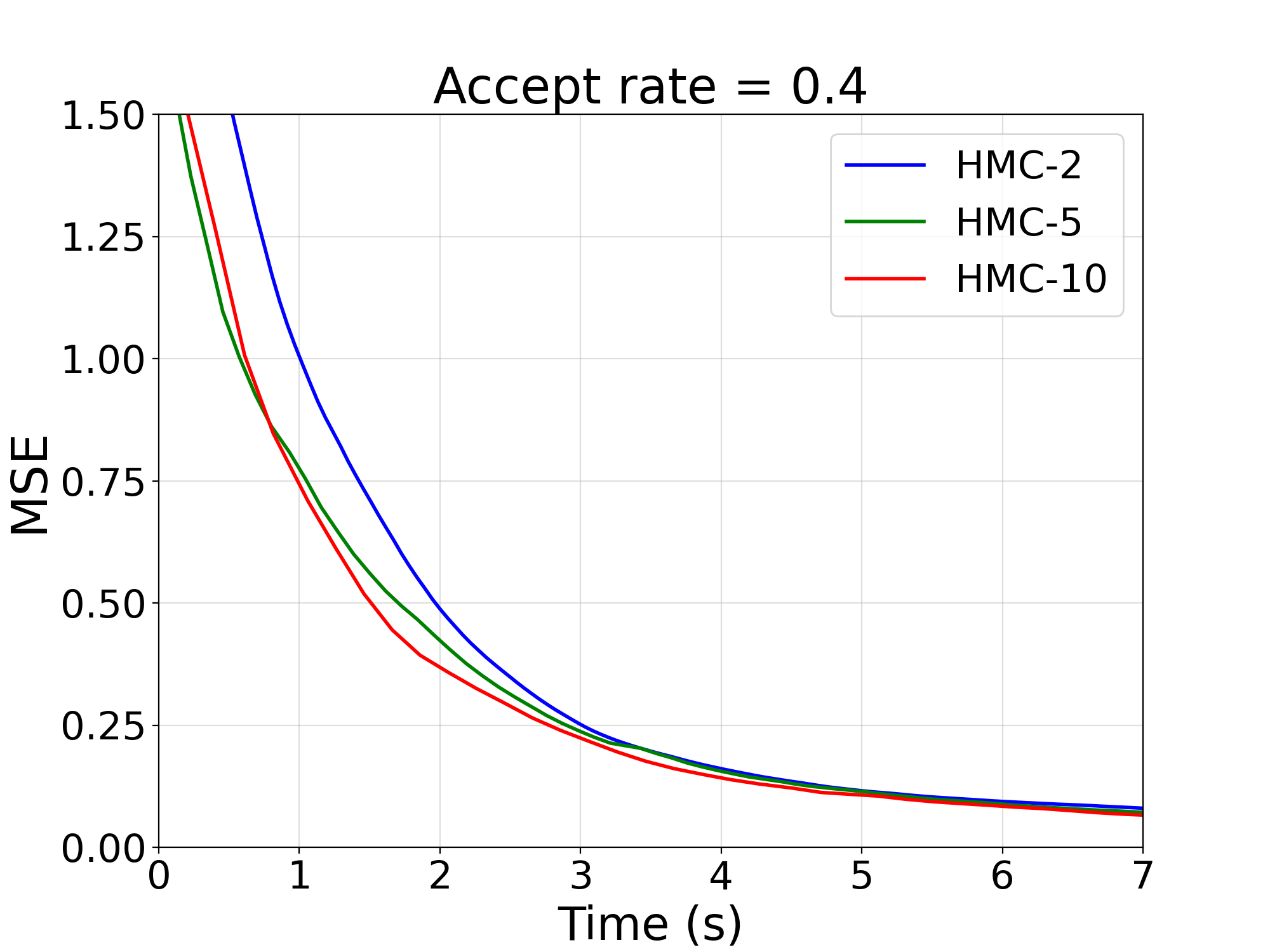
(b) acceptance rate=0.4

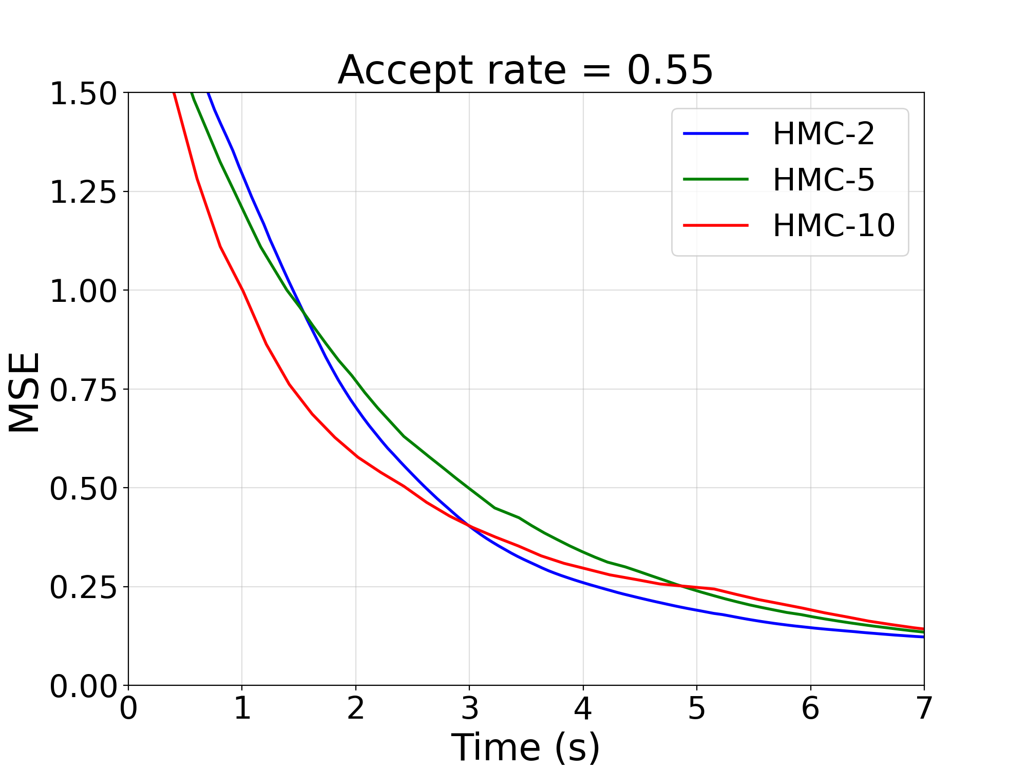
(c) acceptance rate=0.55

Figure 7: Clock-time MSE comparison for HMC with leapfrog steps $2,5,$ and $10$.

E.2 50-dimensional robust linear regression

We compare Poisson-Barker, Poisson-MALA, PoissonMH, random-walk Metropolis, MALA, and HMC in a 50-dimensional robust linear regression example. All setups are the same as in Section 5.2, except for $d=50$, and the number of leapfrog steps in HMC is 5.

Figure 8 shows the MSE of estimating the true coefficients over time. Figure 9 shows the MSE comparison over iteration count. Table 3 compares the ESS/s. Figure 10 compares HMC with 2, 5, and 10 leapfrog steps. The higher dimensionality slows the mixing of all algorithms compared to Section 5.2, but all our conclusions remain valid. Our Poisson–MALA and Poisson–Barker outperform all other algorithms.

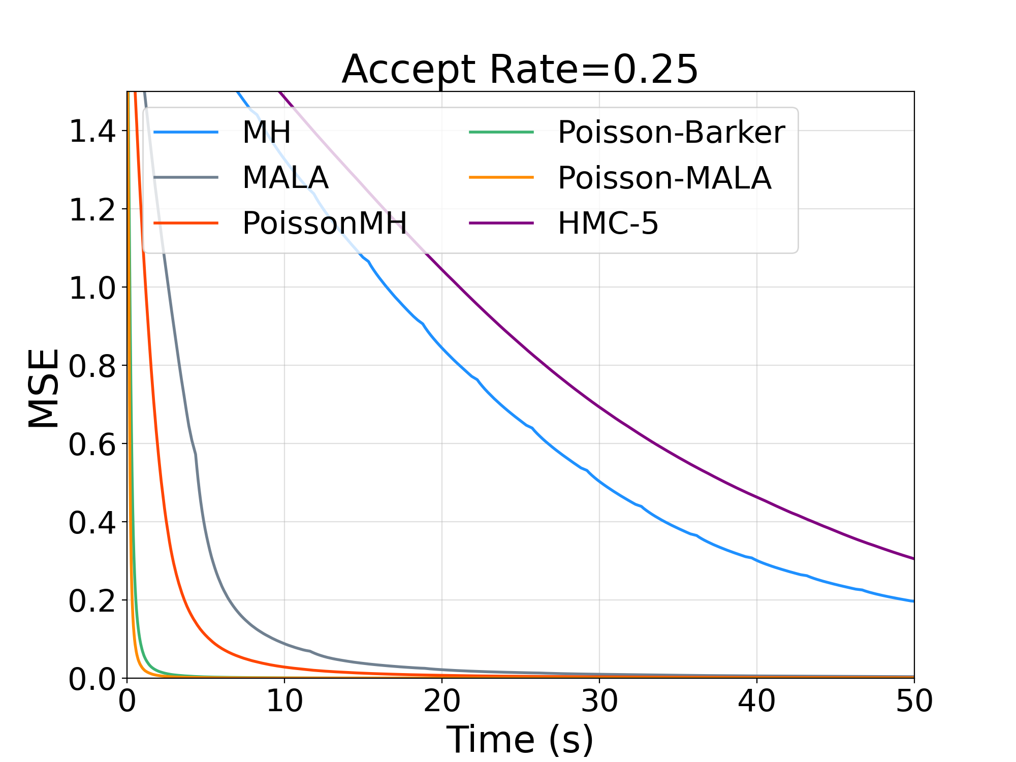
(a) acceptance rate=0.25

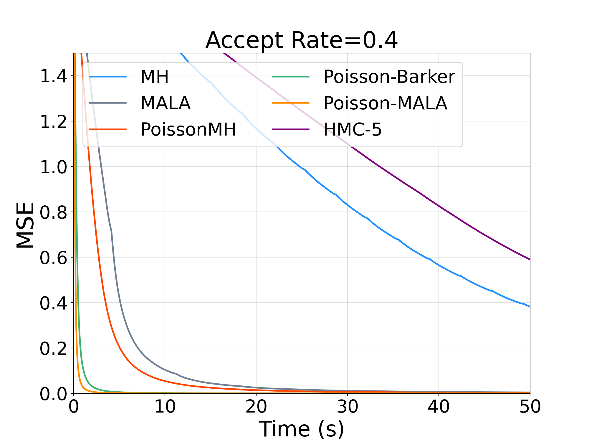
(b) acceptance rate=0.4

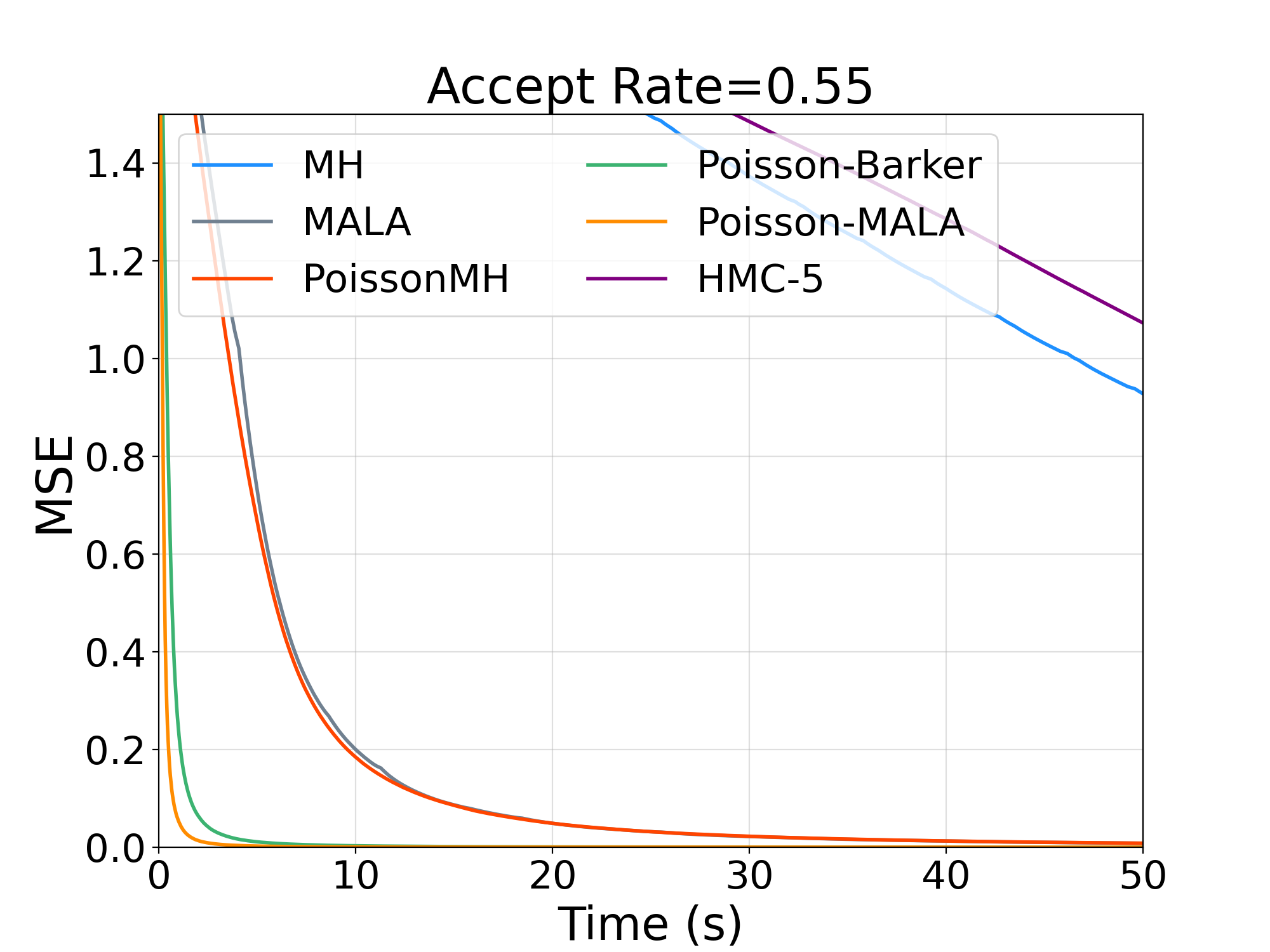
(c) acceptance rate=0.55

Figure 8: Clock-wise MSE comparison. MSE of $\theta^{\star}$ as a function of time across different acceptance rates. The three large plots show the performance of all methods in the first 50 seconds.

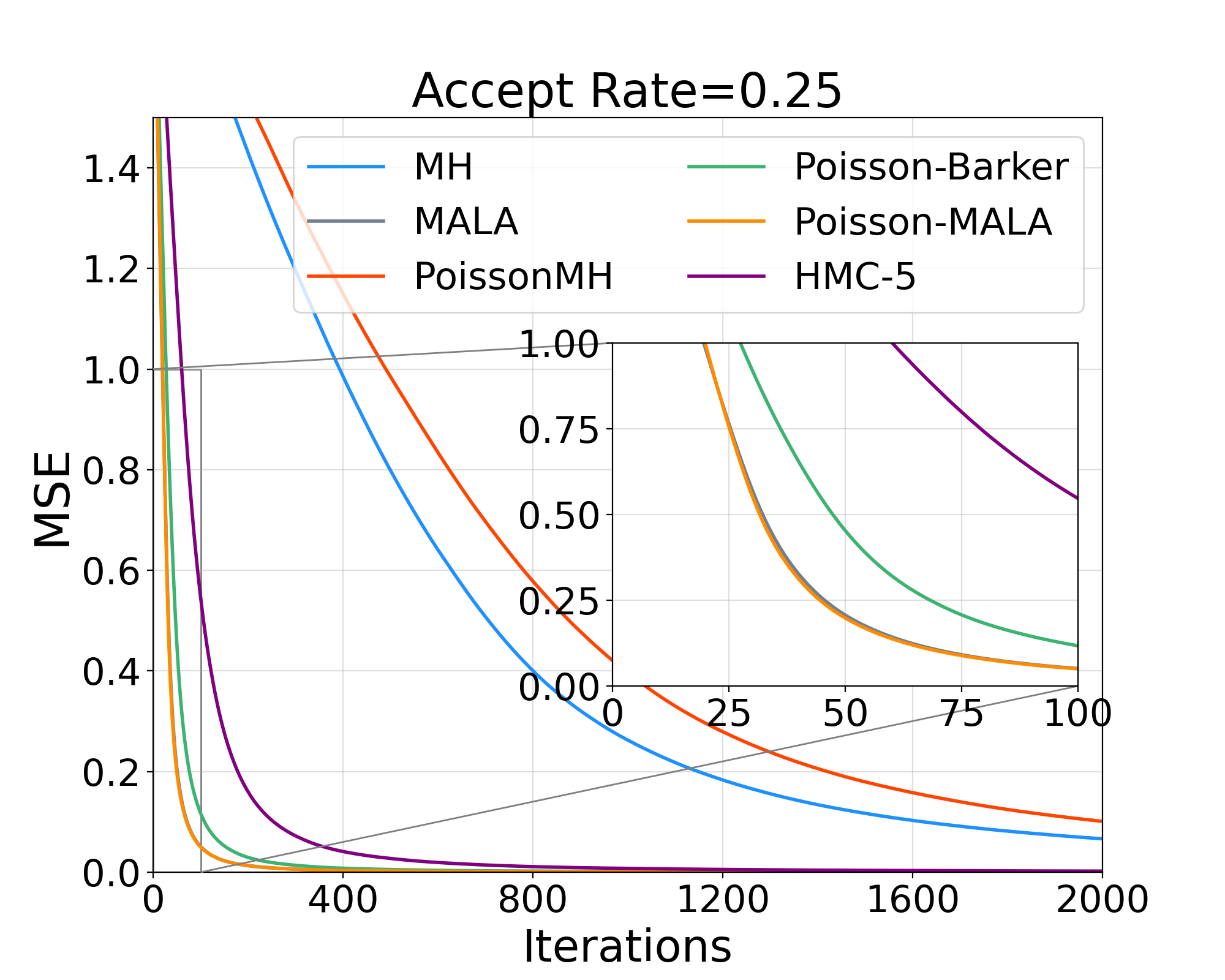
(a) acceptance rate=0.25

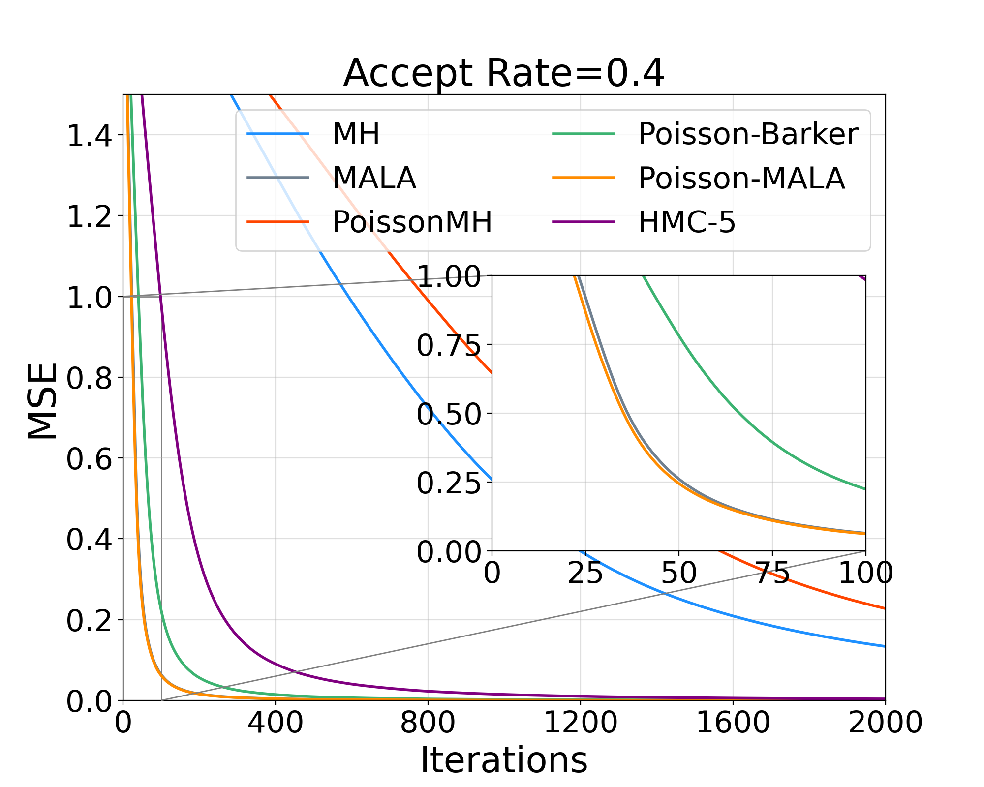
(b) acceptance rate=0.4

(c) acceptance rate=0.55

Figure 9: Iteration-wise MSE comparison. MSE of $\theta^{\star}$ as a function of iteration count different acceptance rates. The three large plots show the performance of all methods in the first 2000 steps. The three inside plots zoom in on Poisson-Barker, and Poisson-MALA, MALA, and HMC in the first 100 steps. All results are averaged over 10 runs.

ESS/s: (Min, Median, Max) Method acceptance rate=0.25 acceptance rate=0.4 acceptance rate=0.55 Best MH (0.09, 0.11, 0.14) (0.08, 0.10, 0.12) (0.06, 0.07, 0.08) (0.09, 0.11, 0.14) MALA (0.40, 0.49, 0.55) (0.77, 0.86, 0.97) (0.82, 0.89, 0.97) (0.82, 0.89, 0.97) HMC-5 (0.04, 0.04, 0.05) (0.04, 0.04, 0.05) (0.03, 0.03, 0.04) (0.04, 0.04, 0.05) PoissonMH (2.12, 2.18, 2.30) (1.85, 1.95, 2.03) (1.36, 1.43, 1.48) (2.12, 2.18, 2.30) PoissonMH-Barker (4.99, 5.25, 5.62) (6.55, 7.05, 7.57) (6.99, 7.37, 7.57) (6.99, 7.37, 7.57) PoissonMH-MALA (8.35, 8.82, 9.16) (13.34, 14.36, 14.81) (15.89, 16.15, 16.58) (15.89, 16.15, 16.58)

Table 3: ESS/s comparison. Here (Min, Median, Max) refer to the minimum, median and maximum of ESS/s across all dimensions. The column “Best” reports the best ESS/s across all acceptance rates. The results are averaged over 10 runs for all five methods.

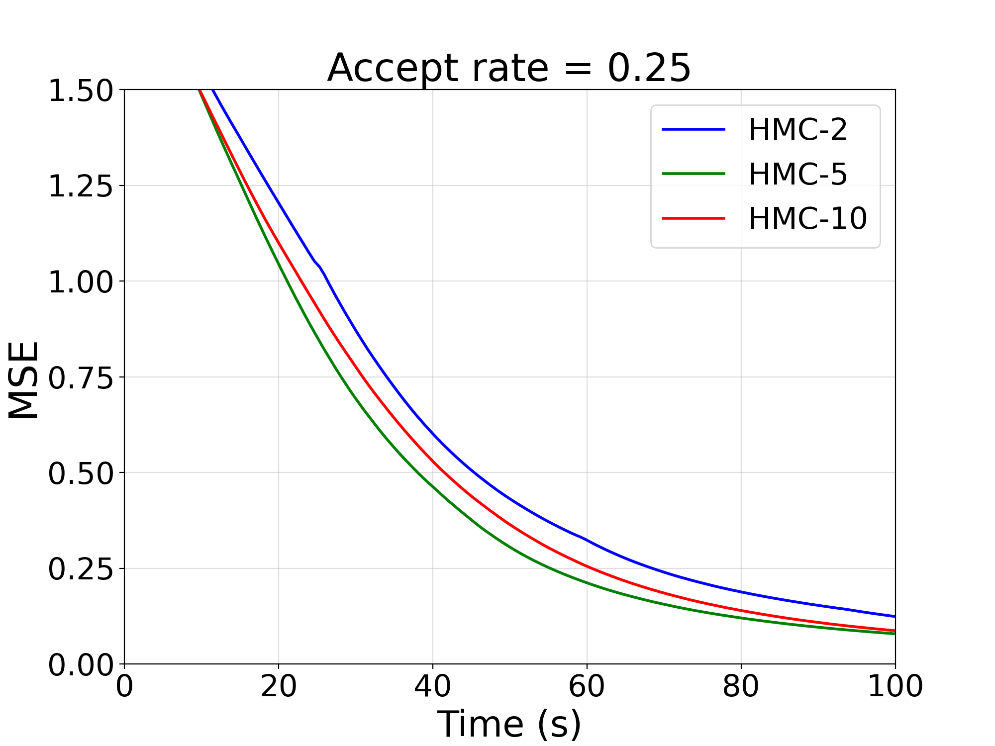
(a) acceptance rate=0.25

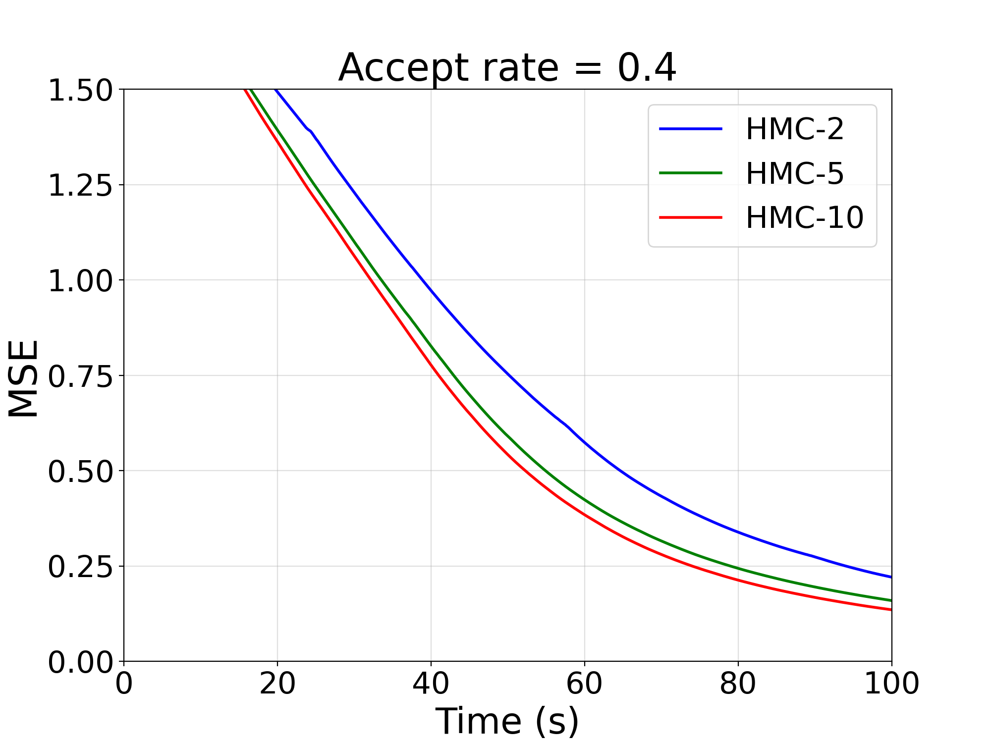
(b) acceptance rate=0.4

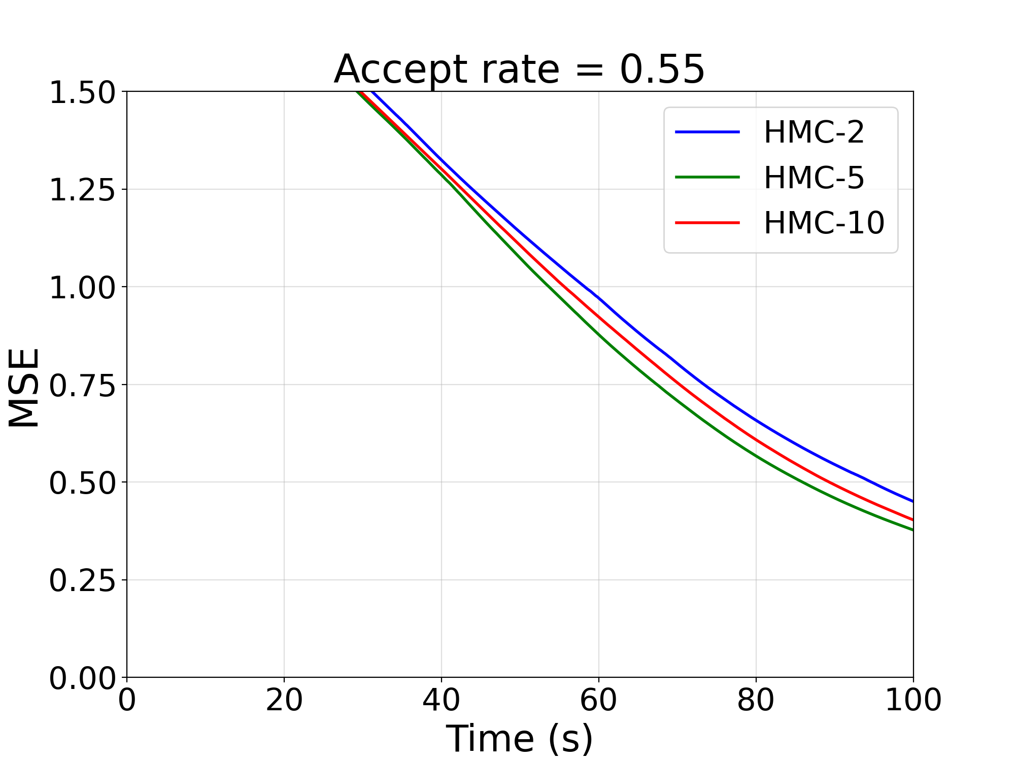
(c) acceptance rate=0.55

Figure 10: Clock-time MSE comparison for HMC with leapfrog steps $2,5,$ and $10$.

E.3 Additional experiments on Bayesian Logistic Regression: 3s and 5s

We compare all five algorithms, along with an additional HMC with 2 leapfrog steps, over a broader range of step sizes, some of which are much larger than those used in Zhang et al., (2020). The test accuracy for each algorithm with varying step sizes is summarised in Figure 11. Increasing the step size overall improves the performance of every full-batch algorithm, especially for HMC. However, the plot clearly shows that the HMC algorithm still struggles with mixing, even with very large step sizes, typically taking more than 30 seconds to converge.

Figure 12 shows a comparison of all six algorithms when each is optimally tuned. From the left panel, it is clear that Tuna–SGLD converges fastest among all algorithms, followed by TunaMH and random-walk Metropolis. The right panel indicates that MALA exhibits superior iteration-wise convergence compared to Tuna–SGLD, while random-walk Metropolis demonstrates better iteration-wise convergence than TunaMH. This observation supports our theoretical findings in Section 4.1.

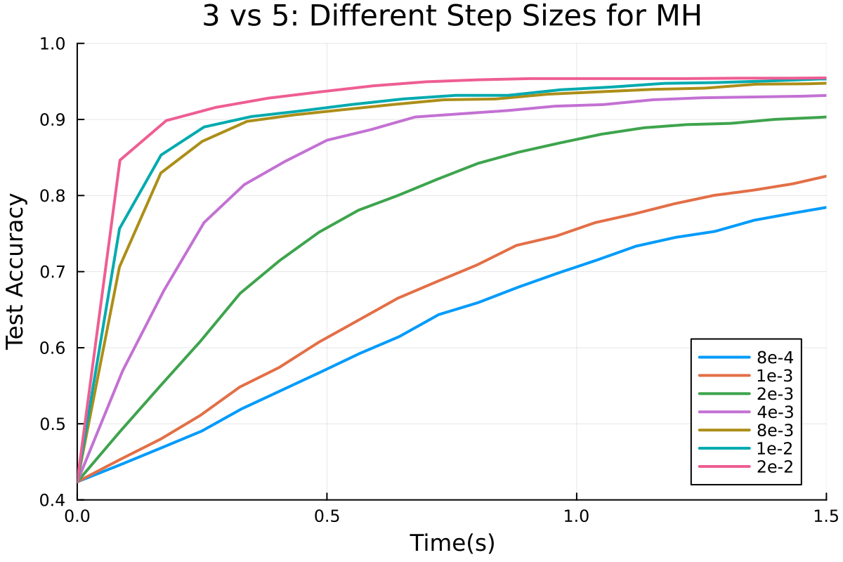
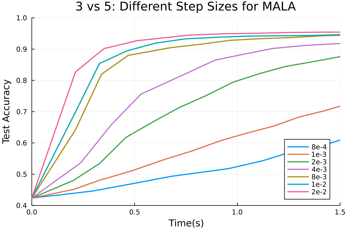
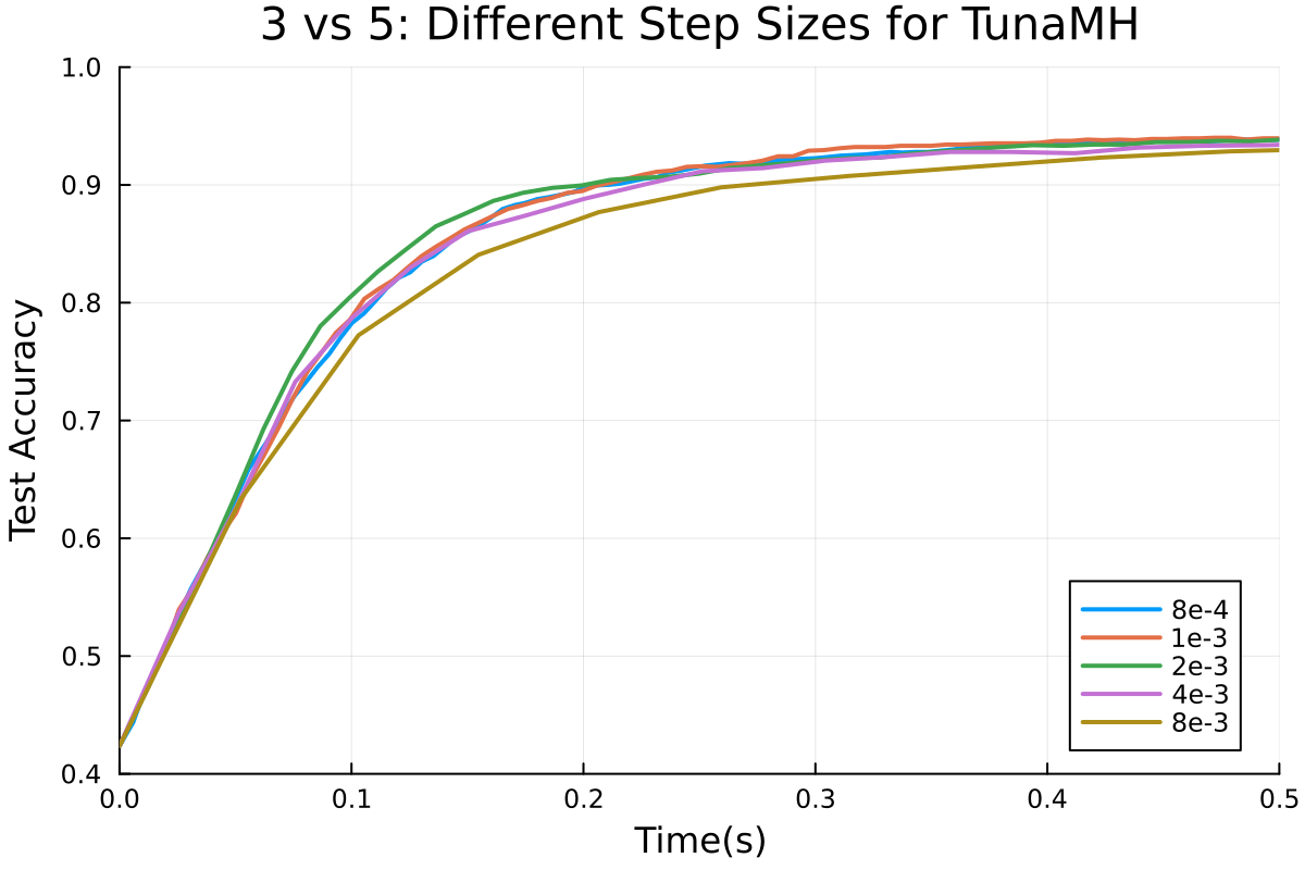
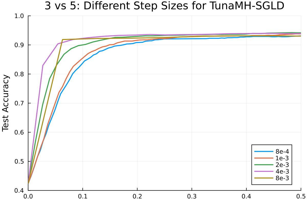
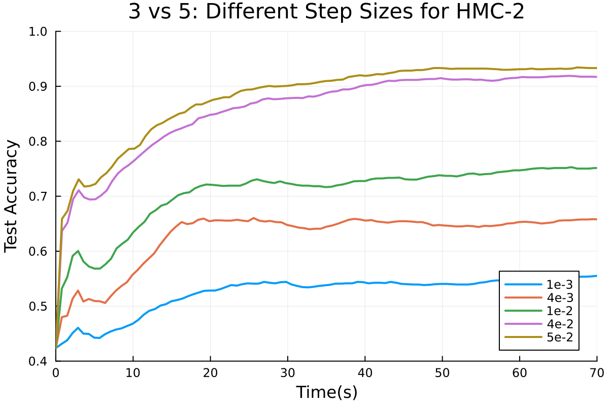
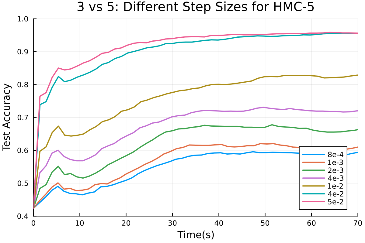
Figure 11: Test accuracy as a function of time for each algorithm with different stepsizes.

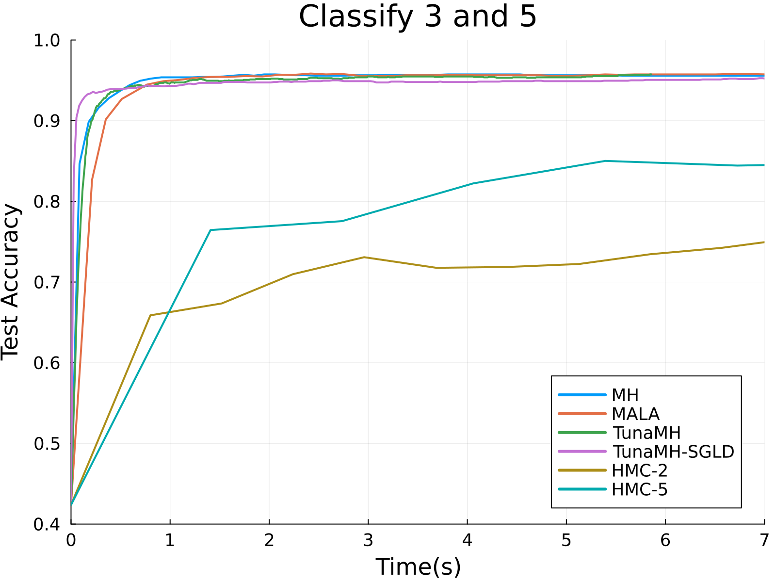
(a) Test accuracy as a function of time

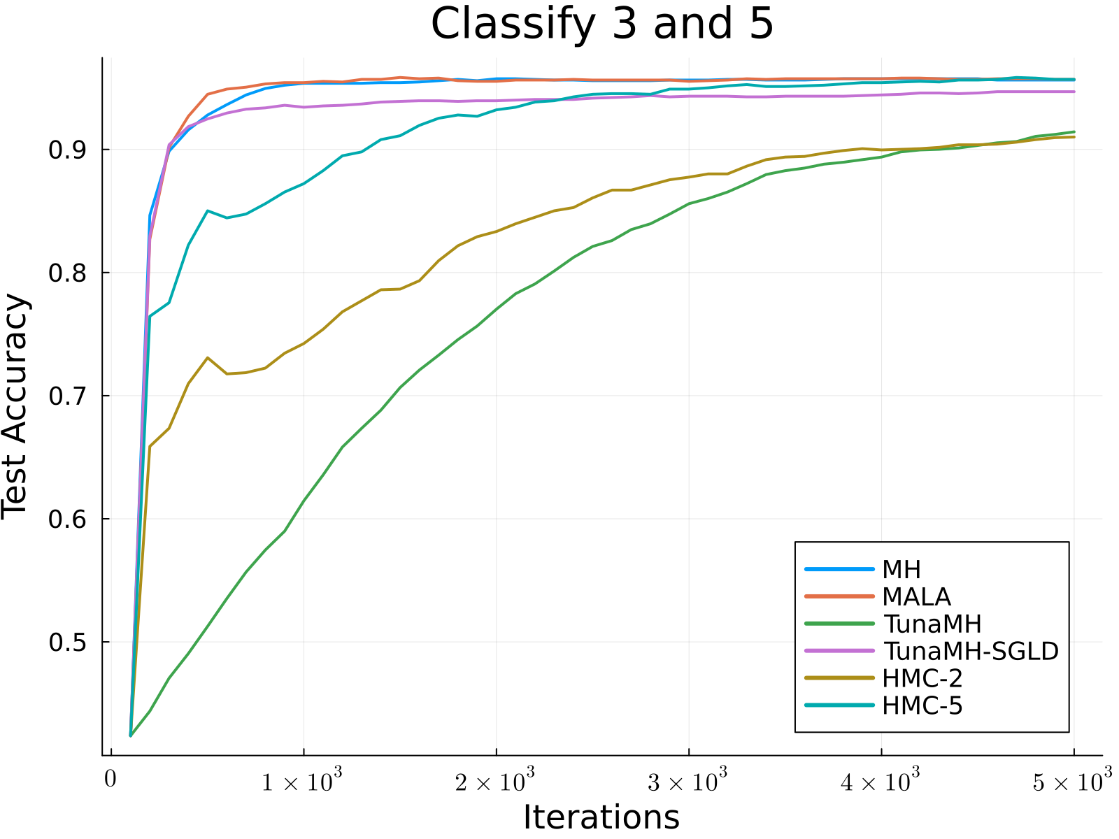
(b) Test accuracy as a function of iteration count

Figure 12: Test accuracy comparison when each algorithm is optimally tuned

E.4 Bayesian Logistic Regression: 7s and 9s

Similar to Section 5.3, we test TunaMH, TunaMH–SGLD, random–walk Metropolis, MALA and HMC on Bayesian logistic regression task to classify 7s and 9s in the MNIST data set. The training set contains 12,214 samples, and the test set contains 2,037 samples. We adopt all implementation details from Section 5.3 and report the results in Figure 13. We can draw similar conclusions to Section 5.3 that our proposed minibatch gradient-based algorithm performs better than its original minibatch non-gradient version in all step size configurations. All minibatch methods still significantly improve the performances of full batch methods.

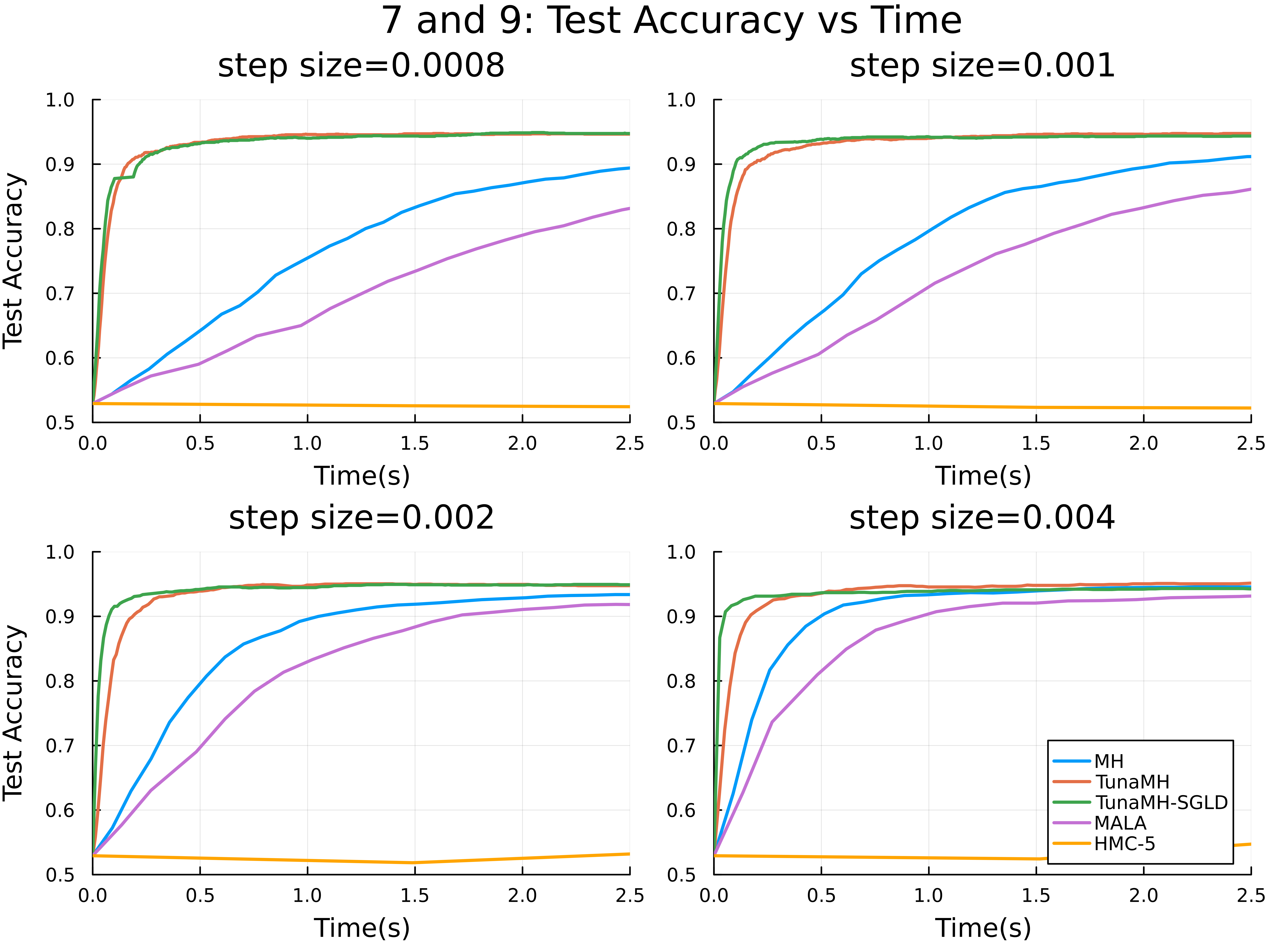
Figure 13: Test accuracy as a function of time for classifying 7s and 9s in MNIST. Step sizes for all methods are varied across $\{0.0008,0.001,0.002,0.004\}$. Each subplot reports the curve of test accuracy in the first 2.5 seconds.

References

- Ahn, (2015) Ahn, S. (2015). Stochastic gradient MCMC: Algorithms and applications. University of California, Irvine.
- Alquier et al., (2016) Alquier, P., Friel, N., Everitt, R., and Boland, A. (2016). Noisy monte carlo: Convergence of markov chains with approximate transition kernels. Statistics and Computing, 26(1-2):29–47.
- (3) Andrieu, C., Doucet, A., Yıldırım, S., and Chopin, N. (2018a). On the utility of Metropolis-Hastings with asymmetric acceptance ratio. arXiv preprint arXiv:1803.09527.
- Andrieu et al., (2022) Andrieu, C., Lee, A., Power, S., and Wang, A. Q. (2022). Comparison of Markov chains via weak Poincaré inequalities with application to pseudo-marginal MCMC. The Annals of Statistics, 50(6):3592–3618.
- Andrieu et al., (2023) Andrieu, C., Lee, A., Power, S., and Wang, A. Q. (2023). Weak Poincaré Inequalities for Markov chains: theory and applications. arXiv preprint arXiv:2312.11689.
- (6) Andrieu, C., Lee, A., and Vihola, M. (2018b). Uniform ergodicity of the iterated conditional SMC and geometric ergodicity of particle Gibbs samplers. Bernoulli, 24(2).
- Andrieu and Roberts, (2009) Andrieu, C. and Roberts, G. O. (2009). The Pseudo-Marginal Approach for Efficient Monte Carlo Computations. The Annals of Statistics, pages 697–725.
- Andrieu and Vihola, (2015) Andrieu, C. and Vihola, M. (2015). Convergence properties of pseudo-marginal Markov chain Monte Carlo algorithms. The Annals of Applied Probability, 25(2):1030–1077.
- Ascolani et al., (2024) Ascolani, F., Roberts, G. O., and Zanella, G. (2024). Scalability of Metropolis-within-Gibbs schemes for high-dimensional Bayesian models. arXiv preprint arXiv:2403.09416.
- Bardenet et al., (2017) Bardenet, R., Doucet, A., and Holmes, C. (2017). On Markov chain Monte Carlo methods for tall data. Journal of Machine Learning Research, 18(47):1–43.
- Barker, (1965) Barker, A. A. (1965). Monte Carlo calculations of the radial distribution functions for a proton electron plasma. Australian Journal of Physics, 18(2):119–134.
- Beaumont, (2003) Beaumont, M. A. (2003). Estimation of population growth or decline in genetically monitored populations. Genetics, 164(3):1139–1160.
- Besag, (1974) Besag, J. (1974). Spatial interaction and the statistical analysis of lattice systems. Journal of the Royal Statistical Society: Series B (Methodological), 36(2):192–225.
- Besag, (1986) Besag, J. (1986). On the statistical analysis of dirty pictures. Journal of the Royal Statistical Society Series B: Statistical Methodology, 48(3):259–279.
- Besag, (1994) Besag, J. (1994). Comments on “Representations of knowledge in complex systems” by U. Grenander and MI Miller. J. Roy. Statist. Soc. Ser. B, 56(591-592):4.
- Bierkens et al., (2019) Bierkens, G., Fearnhead, P., and Roberts, G. (2019). The Zig-Zag process and super-efficient sampling for Bayesian analysis of big data. Annals of Statistics, 47(3).
- Bouchard-Côté et al., (2018) Bouchard-Côté, A., Vollmer, S. J., and Doucet, A. (2018). The bouncy particle sampler: A nonreversible rejection-free Markov chain Monte Carlo method. Journal of the American Statistical Association, 113(522):855–867.
- Bretagnolle and Huber, (1979) Bretagnolle, J. and Huber, C. (1979). Estimation des densités: risque minimax. Zeitschrift für Wahrscheinlichkeitstheorie und verwandte Gebiete, 47:119–137.
- Campbell and Broderick, (2018) Campbell, T. and Broderick, T. (2018). Bayesian coreset construction via greedy iterative geodesic ascent. In International Conference on Machine Learning, pages 698–706. PMLR.
- Campbell and Broderick, (2019) Campbell, T. and Broderick, T. (2019). Automated scalable bayesian inference via hilbert coresets. Journal of Machine Learning Research, 20(15):1–38.
- Canonne, (2022) Canonne, C. L. (2022). A short note on an inequality between kl and tv. arXiv preprint arXiv:2202.07198.
- Chen et al., (2014) Chen, T., Fox, E., and Guestrin, C. (2014). Stochastic gradient hamiltonian monte carlo. In International Conference on Machine Learning, pages 1683–1691. PMLR.
- Cornish et al., (2019) Cornish, R., Vanetti, P., Bouchard-Côté, A., Deligiannidis, G., and Doucet, A. (2019). Scalable metropolis-hastings for exact bayesian inference with large datasets. In International Conference on Machine Learning, pages 1351–1360. PMLR.
- Dang et al., (2019) Dang, K.-D., Quiroz, M., Kohn, R., Tran, M.-N., and Villani, M. (2019). Hamiltonian Monte Carlo with energy conserving subsampling. Journal of Machine Learning Research, 20(100):1–31.
- Diaconis and Saloff-Coste, (1993) Diaconis, P. and Saloff-Coste, L. (1993). Comparison theorems for reversible Markov chains. The Annals of Applied Probability, 3(3):696–730.
- Diaconis and Wang, (2018) Diaconis, P. and Wang, G. (2018). Bayesian goodness of fit tests: a conversation for david mumford. Annals of Mathematical Sciences and Applications, 3(1):287–308.
- Duane et al., (1987) Duane, S., Kennedy, A. D., Pendleton, B. J., and Roweth, D. (1987). Hybrid monte carlo. Physics letters B, 195(2):216–222.
- Dwivedi et al., (2019) Dwivedi, R., Chen, Y., Wainwright, M. J., and Yu, B. (2019). Log-concave sampling: Metropolis-Hastings algorithms are fast. Journal of Machine Learning Research, 20(183):1–42.
- Dyer et al., (2006) Dyer, M., Goldberg, L. A., Jerrum, M., and Martin, R. (2006). Markov chain comparison. Probability Surveys, 3:89–111.
- Fearnhead et al., (2010) Fearnhead, P., Papaspiliopoulos, O., Roberts, G. O., and Stuart, A. (2010). Random-weight particle filtering of continuous time processes. Journal of the Royal Statistical Society Series B: Statistical Methodology, 72(4):497–512.
- Gelman et al., (2008) Gelman, A., Jakulin, A., Pittau, M. G., and Su, Y.-S. (2008). A weakly informative default prior distribution for logistic and other regression models. The Annals of Applied Statistics, 2(4):1360 – 1383.
- Gerchinovitz et al., (2020) Gerchinovitz, S., Ménard, P., and Stoltz, G. (2020). Fano’s inequality for random variables. Statistical Science, 35(2):178–201.
- Hastings, (1970) Hastings, W. (1970). Monte Carlo sampling methods using Markov chains and their applications. Biometrika, 57(1):97–109.
- Hoff, (2009) Hoff, P. D. (2009). Simulation of the matrix bingham–von mises–fisher distribution, with applications to multivariate and relational data. Journal of Computational and Graphical Statistics, 18(2):438–456.
- Huang and Gelman, (2005) Huang, Z. and Gelman, A. (2005). Sampling for bayesian computation with large datasets. Available at SSRN 1010107.
- Huggins et al., (2016) Huggins, J., Campbell, T., and Broderick, T. (2016). Coresets for scalable Bayesian logistic regression. Advances in neural information processing systems, 29.
- Jacob and Thiery, (2015) Jacob, P. E. and Thiery, A. H. (2015). On nonnegative unbiased estimators. The Annals of Statistics, pages 769–784.
- Johndrow et al., (2020) Johndrow, J. E., Pillai, N. S., and Smith, A. (2020). No free lunch for approximate mcmc. arXiv preprint arXiv:2010.12514.
- Korattikara et al., (2014) Korattikara, A., Chen, Y., and Welling, M. (2014). Austerity in MCMC land: Cutting the Metropolis-Hastings budget. In International conference on machine learning, pages 181–189. PMLR.
- Łatuszyński and Rudolf, (2014) Łatuszyński, K. and Rudolf, D. (2014). Convergence of hybrid slice sampling via spectral gap. arXiv preprint arXiv:1409.2709.
- Liang, (2010) Liang, F. (2010). A double Metropolis–Hastings sampler for spatial models with intractable normalizing constants. Journal of Statistical Computation and Simulation, 80(9):1007–1022.
- Liang et al., (2016) Liang, F., Jin, I. H., Song, Q., and Liu, J. S. (2016). An adaptive exchange algorithm for sampling from distributions with intractable normalizing constants. Journal of the American Statistical Association, 111(513):377–393.
- Lin et al., (2000) Lin, L., Liu, K., and Sloan, J. (2000). A noisy Monte Carlo algorithm. Physical Review D, 61(7):074505.
- Livingstone and Zanella, (2022) Livingstone, S. and Zanella, G. (2022). The Barker Proposal: Combining Robustness and Efficiency in Gradient-Based MCMC. Journal of the Royal Statistical Society Series B: Statistical Methodology, 84(2):496–523.
- Lyne et al., (2015) Lyne, A.-M., Girolami, M., Atchadé, Y., Strathmann, H., and Simpson, D. (2015). On russian roulette estimates for bayesian inference with doubly-intractable likelihoods. Statistical Science, 30(4):443–467.
- Maclaurin and Adams, (2014) Maclaurin, D. and Adams, R. P. (2014). Firefly monte carlo: Exact mcmc with subsets of data. In Conference on Uncertainty in Artificial Intelligence.
- Martin et al., (2024) Martin, G. M., Frazier, D. T., and Robert, C. P. (2024). Computing Bayes: From Then ‘Til Now. Statistical Science, 39(1):3 – 19.
- Metropolis et al., (1953) Metropolis, N., Rosenbluth, A. W., Rosenbluth, M. N., Teller, A. H., and Teller, E. (1953). Equation of state calculations by fast computing machines. The Journal of Chemical Physics, 21(6):1087–1092.
- Møller et al., (2006) Møller, J., Pettitt, A. N., Reeves, R., and Berthelsen, K. K. (2006). An efficient Markov chain Monte Carlo method for distributions with intractable normalising constants. Biometrika, 93(2):451–458.
- Murray et al., (2006) Murray, I., Ghahramani, Z., and MacKay, D. J. (2006). Mcmc for doubly-intractable distributions. In Proceedings of the Twenty-Second Conference on Uncertainty in Artificial Intelligence, pages 359–366.
- Neal et al., (2011) Neal, R. M. et al. (2011). MCMC using Hamiltonian dynamics. Handbook of markov chain monte carlo, 2(11):2.
- Neiswanger et al., (2014) Neiswanger, W., Wang, C., and Xing, E. P. (2014). Asymptotically exact, embarrassingly parallel mcmc. In Proceedings of the Thirtieth Conference on Uncertainty in Artificial Intelligence, pages 623–632.
- Nicholls et al., (2012) Nicholls, G. K., Fox, C., and Watt, A. M. (2012). Coupled MCMC with a randomized acceptance probability. arXiv preprint arXiv:1205.6857.
- Papaspiliopoulos, (2011) Papaspiliopoulos, O. (2011). Monte Carlo probabilistic inference for diffusion processes: a methodological framework, page 82–103. Cambridge University Press.
- Peskun, (1973) Peskun, P. H. (1973). Optimum monte-carlo sampling using markov chains. Biometrika, 60(3):607–612.
- Power et al., (2024) Power, S., Rudolf, D., Sprungk, B., and Wang, A. Q. (2024). Weak Poincaré inequality comparisons for ideal and hybrid slice sampling. arXiv preprint arXiv:2402.13678.
- Qin et al., (2023) Qin, Q., Ju, N., and Wang, G. (2023). Spectral gap bounds for reversible hybrid Gibbs chains. arXiv preprint arXiv:2312.12782.
- Quiroz et al., (2018) Quiroz, M., Kohn, R., Villani, M., and Tran, M.-N. (2018). Speeding up MCMC by efficient data subsampling. Journal of the American Statistical Association.
- Rao et al., (2016) Rao, V., Lin, L., and Dunson, D. B. (2016). Data augmentation for models based on rejection sampling. Biometrika, 103(2):319–335.
- Robins et al., (2007) Robins, G., Pattison, P., Kalish, Y., and Lusher, D. (2007). An introduction to exponential random graph () models for social networks. Social networks, 29(2):173–191.
- Seita et al., (2018) Seita, D., Pan, X., Chen, H., and Canny, J. (2018). An efficient minibatch acceptance test for metropolis-hastings. In Proceedings of the 27th International Joint Conference on Artificial Intelligence, pages 5359–5363.
- Strauss, (1975) Strauss, D. J. (1975). A model for clustering. Biometrika, 62(2):467–475.
- Tierney, (1998) Tierney, L. (1998). A note on metropolis-hastings kernels for general state spaces. Annals of Applied Probability, pages 1–9.
- Titsias and Papaspiliopoulos, (2018) Titsias, M. K. and Papaspiliopoulos, O. (2018). Auxiliary gradient-based sampling algorithms. Journal of the Royal Statistical Society Series B: Statistical Methodology, 80(4):749–767.
- Vitelli et al., (2018) Vitelli, V., Sørensen, Ø., Crispino, M., Frigessi, A., and Arjas, E. (2018). Probabilistic preference learning with the Mallows rank model. Journal of Machine Learning Research, 18(158):1–49.
- Vogrinc et al., (2023) Vogrinc, J., Livingstone, S., and Zanella, G. (2023). Optimal design of the barker proposal and other locally balanced Metropolis–Hastings algorithms. Biometrika, 110(3):579–595.
- Vollmer et al., (2016) Vollmer, S. J., Zygalakis, K. C., and Teh, Y. W. (2016). Exploration of the (non-) asymptotic bias and variance of stochastic gradient langevin dynamics. Journal of Machine Learning Research, 17(159):1–48.
- Wagner, (1987) Wagner, W. (1987). Unbiased Monte Carlo evaluation of certain functional integrals. Journal of Computational Physics, 71(1):21–33.
- Wang, (2022) Wang, G. (2022). On the theoretical properties of the exchange algorithm. Bernoulli, 28(3):1935 – 1960.
- Wang and Dunson, (2013) Wang, X. and Dunson, D. B. (2013). Parallelizing MCMC via Weierstrass sampler. arXiv preprint arXiv:1312.4605.
- Welling and Teh, (2011) Welling, M. and Teh, Y. W. (2011). Bayesian learning via stochastic gradient langevin dynamics. In Proceedings of the 28th international conference on machine learning (ICML-11), pages 681–688.
- Wu et al., (2022) Wu, T.-Y., Rachel Wang, Y., and Wong, W. H. (2022). Mini-batch Metropolis–Hastings with reversible SGLD proposal. Journal of the American Statistical Association, 117(537):386–394.
- Zanella, (2020) Zanella, G. (2020). Informed proposals for local mcmc in discrete spaces. Journal of the American Statistical Association, 115(530):852–865.
- Zhang et al., (2020) Zhang, R., Cooper, A. F., and De Sa, C. M. (2020). Asymptotically optimal exact minibatch Metropolis–Hastings. Advances in Neural Information Processing Systems, 33:19500–19510.
- Zhang and De Sa, (2019) Zhang, R. and De Sa, C. M. (2019). Poisson-minibatching for gibbs sampling with convergence rate guarantees. Advances in Neural Information Processing Systems, 32.