Recursive Landau Analysis

Abstract

We propose a recursive method that makes use of the basic principle of unitarity to calculate the Landau singularities of $n$-point scattering amplitudes directly in kinematic space. For a vast class of Feynman diagrams, the method enables rapid analytic computation of Landau singularities beyond current state-of-the-art technology. This includes new predictions relevant for two- and higher-loop processes in the Standard Model involving both massive quarks and electroweak particles.

1   Introduction

Scattering amplitudes are fascinating objects [1] that characterize the interactions of relativistic particles and can be used to determine cross-section and other useful physical observables. They exhibit a rich analytic structure as a function of the momenta of the scattered particles.

In weakly coupled quantum field theories, such as the Standard Model at high energies, the Feynman diagram expansion offers a systematic way to organize calculations of amplitudes and to study their analytic structure. Despite a great deal of understanding, the computation of Feynman integrals remains a difficult task that often becomes intractable at high orders, particularly when massive particles are involved (see [2] for a recent overview).

Knowing beforehand the singularity structure of a Feynman integral greatly helps in its computation and may even suffice to “bootstrap” the result when combined with additional physical constraints and a good control over the function space (e.g., polylogaritms and their elliptic analogues [3]). This principle has proven to be especially rewarding for planar $\mathcal{N}=4$ super Yang–Mills amplitudes, where amplitudes have been obtained to high multiplicity and loop orders [4, 5, 6, 7, 8, 9, 10]. It is also starting to be used for integrals in more realistic theories [11, 12, 13, 14, 15, 16].

The singularity locus of a Feynman integral can be studied without having to first compute it, as Landau proposed in his seminal paper [17]. The Landau equations [18, Eq. (1)] are a set of necessary algebraic conditions for the existence of a singularity of the Feynman integral. Unsurprisingly, their complexity also increases with the number of loops, external particles, and mass scales. The current state-of-the-art makes use of modern algebraic geometry techniques to compute two-loop examples relevant for Standard Model processes [19, 18, 20] (see [21, 15, 22, 23, 24, 25, 26, 27, 28, 29, 30, 31]).

The Landau singularities of Feynman integrals are purely kinematical and are believed to exist beyond the weak-coupling approximation that underlies the Feynman diagrammatic expansion. It was already noted in the 1960s by Mandelstam and others [32, 33, 34] (see [35, 28, 36, 37] for recent accounts) that general principles such as unitarity and crossing symmetry require the full non-perturbative amplitude to be singular at the same locations as the Landau singularities found for some Feynman diagrams.

Here, we bring together valuable insights from both approaches. We propose a recursive method for the calculation of Landau singularities exploiting the general principle of unitarity.

2   Recursion via unitarity

A Feynman graph $G$ with $n$ external legs is a function on the kinematic space consisting of Lorentz-invariant combinations of momenta $X_{G}=\{p_{i}{\cdot}p_{j}\}_{i,j=1}^{n-1}$ and internal masses. Its codimension-one singularities are characterized by a list ${\cal L}(G)$ of polynomials in these variables

$${\cal L}(G)_{i}=0\,.$$ (1)

Our goal is to compute these polynomials recursively in terms of those of subgraphs. The product $\prod_{i}{\cal L}(G)_{i}$ is called the (principal) Landau discriminant in [19, 18, 20]. Before discussing complex singularities, we start by revisiting the relation between singularities and cuts for real momenta.

Unitarity and thresholds.

Unitarity is the basic quantum mechanical requirement that probabilities sum up to unity. In terms of the S-matrix, which evolves states from the far past to the far future, it reads $SS^{\dagger}=\mathbbm{1}$. By the usual separation between free and interacting parts ($S{=}\mathbbm{1}{+}iT$), it implies that $2\mathrm{Im}\,T=TT^{\dagger}$.

Scattering amplitudes are the matrix elements of $T$: $\mathscr{M}_{n_{A}\to n_{B}}=\langle n_{B}|T|n_{A}\rangle$, where $|n_{A}\rangle$ and $|n_{B}\rangle$ denote $n_{A}$- and $n_{B}$-particle momentum eigenstates. In terms of matrix elements, unitarity yields an infinite system of coupled integral equations (see e.g., [38, Ch. 2])

$$2\mathrm{Im}\,\mathscr{M}_{n_{A}\to n_{B}}=\operatorname*{\mathchoice{\ooalign{$\displaystyle\sum$\cr$\displaystyle\int$\cr}}{\ooalign{\raisebox{0.14pt}{\scalebox{0.7}{$\textstyle\sum$}}\cr$\textstyle\int$\cr}}{\ooalign{\raisebox{0.2pt}{\scalebox{0.6}{$\scriptstyle\sum$}}\cr$\scriptstyle\int$\cr}}{\ooalign{\raisebox{0.2pt}{\scalebox{0.6}{$\scriptstyle\sum$}}\cr$\scriptstyle\int$\cr}}}_{X}\mathscr{M}_{n_{A}\to X}\leavevmode\nobreak\ \mathscr{M}^{*}_{X\to n_{B}}\,,$$ (2)

where the integral is over the on-shell phase space of the intermediate $X$-particle state. In perturbation theory, (2) leads to the well-known Cutkosky equation [39], which relates the imaginary part of a given Feynman diagram to the sum over all cuts that divide it into two or more disconnected subgraphs; each cut particle being on-shell.

We will need the case where a two-particle cut separates a graph $AB$ into two subgraphs $A$ and $B$. The invariants on each side of the cut are

$$X_{\xi}=\{q_{i}\cdot q_{j}\mid q_{\bullet}\in\{k\}\cup P_{\xi}\}\quad(\xi=A,B)\,,$$ (3)

where $P_{A}=\{p_{i}\}_{i=1}^{a}$ and $P_{B}=\{p_{i}\}_{i=a+1}^{n}$. Below, we also adopt $p_{I}$ to denote the sum $p_{I}\equiv\sum_{i\in I}p_{i}$ (where $I$ is a multi-index) and $s_{I}\equiv p_{I}^{2}$ for Mandelstam invariants. We also ignore numerators and spin, as they do not affect the locations of possible Landau singularities.

Following Mandelstam [40] or the more general Baikov representation [41, 42], the cut integral can be written in terms of these invariants (assuming that positive energy-flow along the cut is possible, see [38, Eq. (2.29)]):

$$\scalebox{0.75}[0.75]{\leavevmode\hbox{$\vbox{\hbox{\resizebox{}{}{{\leavevmode\hbox{\set@color{ \leavevmode\hbox to129.81pt{\vbox to59.73pt{\text{[drawing]}}} }}}}}}$}}=C\int_{\Gamma}{\mathrm{d}\mu A(X_{A})\,B(X_{B})\over\det\mathcal{G}(Q)^{\frac{n+1-\mathrm{D}}{2}}}\,, p_{1} \vdots p_{a} p_{n} \vdots p_{a+1} k A B \mathrm{Cut}_{AB}(P_{A},P_{B}) p_{1} \vdots p_{a} p_{n} \vdots p_{a+1} k A B \mathrm{Cut}_{AB}(P_{A},P_{B})$$ (4)

where $\mathcal{G}(P)$ denotes the Gram matrix of dot products between vectors in the set $P$ and

$$\begin{split}\mathrm{d}\mu&=\prod_{Q_{i}\in Q}\mathrm{d}(k\cdot Q_{i})\delta[k^{2}{-}m_{k}^{2}]\,\delta[(k{+}p_{1\ldots a})^{2}{-}m_{k^{\prime}}^{2}]\,,\\ C&=\det\mathcal{G}(P_{A}{\cup}P_{B}^{\prime})^{\frac{n-\mathrm{D}}{2}}/\sqrt{\pi}\,,\leavevmode\nobreak\ Q=\{k\}{\cup}P_{A}{\cup}P^{\prime}_{B}\,,\end{split}$$ (5)

with $P_{B}^{\prime}=P_{B}\setminus\{p_{n}\}$. The integration domain is

$$\Gamma=\Big{\{}k\cdot Q_{i}\,\Big{|}\,\frac{\det\mathcal{G}(Q)}{\det\mathcal{G}(P_{A}{\cup}P_{B}^{\prime})}>0,Q_{i}\in Q\Big{\}}\,.$$ (6)

The delta functions in (4) can be used to fix two scalar products in $X_{A}$ (one being $k^{2}$). Since there are $n_{A}{=}a$ initial particles and $n_{B}{=}(n{-}a)$ final particles, the final integration is over $(n_{A}{+}n_{B}{-}2)$ variables.

The locations in kinematic space where a cut such as (4) starts contributing to (2) are called thresholds. At these locations, the amplitude cannot be real analytic, and we say that it is singular.

Landau’s analysis shows that all singularities of a diagram are associated with processes in which a subset of its propagators become on-shell. We will focus on the leading singularities of a graph $G$—those in which all propagators are on-shell—since other singularities can be found by looping over subtopologies (with contracted edges).

Necessary conditions for singularities

A scattering amplitude becomes singular when a cut either (i) develops support or (ii) develops a singularity itself. Necessary conditions for this will be phrased algebraically without reference to the reality or positivity of energies.

We first expand on possibility (i). At thresholds, the phase space $\Gamma$ “closes down” to an isolated point such that only classical scattering is possible. This serves as the physical basis for the Coleman–Norton picture of singularities [43]. A necessary condition for this to occur is that the boundary $\partial\Gamma$ (determined by the polynomial $\det\mathcal{G}{=}0$) contracts from all directions. Once localized to $\partial\Gamma$ and the two-particle cut, this can happen only if $\partial_{k{\cdot}p_{i}}\det\mathcal{G}{=}0$ for all remaining integration variables $\{k\cdot p_{i}\}$.

Possibility (ii) has a natural interpretation in terms of contour pinching. Indeed, it is well known that an integral may only diverge if two or more singularities of the integrand pinch the contour of integration [44]. This can happen in two ways for the integral in (4):

1. Singularities from $A$ or $B$ pinch $\partial\Gamma$.

2. Singularities from $A$ or $B$ pinch $\Gamma$.

Visually, conditions (i), (ii^′) and (ii^′′) look like:

In the Baikov representation (4), $A$ and $B$ do not share any common variable on the cut. Therefore, condition (ii^′′) can only involve either $A$ or $B$ separately (with the other being a pure vertex in order for the singularity to be leading). We did not encounter this possibility, so we will not discuss (ii^′′) singularities further. On $\partial\Gamma$, the $A$ and $B$ variables communicate non-trivially through the condition $\det\mathcal{G}=0$.

The necessary conditions (i) and (ii^′) for $AB$ to have a singularity can be written uniformly by picking a possibly empty subset $\mathscr{S}\subset\mathscr{L}(A)\cup\mathscr{L}(B)$ of the singularities of the left and right subamplitudes. Localizing on the two-particle cut and the loci $\{\mathscr{S}_{i}=0\}$ allows to eliminate $\dim(\mathscr{S})$ variables from (4), leaving a set $X_{\mathscr{S}}$ of independent variables in terms of which $\partial\Gamma$ is determined by

$$0=\det\tilde{\mathcal{G}}(X_{\mathscr{S}})\equiv\det\mathcal{G}|_{\{\mathscr{S}_{i}=0\}}\,.$$ (8)

To ensure that there are no directions along which the integration contour could be deformed to avoid the singularity, $\det\tilde{\mathcal{G}}$ and all its derivatives with respect to remaining variables must vanish:

$$\mathscr{L}(AB)_{\mathscr{S}}:\left[\begin{array}[]{@{}l@{\quad}l@{}}\;\det\tilde{\mathcal{G}}=0\vspace{1mm}\\ \displaystyle{\partial\det\tilde{\mathcal{G}}\over\partial(k\cdot p_{i})}=0\end{array}\right.\text{ for }\;k{\cdot}p_{i}\in X_{\mathscr{S}}\,.$$ (9)

Since there is always one more equation than unknowns in (9), evaluating one on the support of the others yields an algebraic constraint $\mathscr{L}(AB)_{\mathscr{S}}=0$ in kinematic space.

To find all candidate leading singularities of a graph $G$ that contains a two-particle cut, it suffices to consider all sets $\mathscr{S}$ of candidate leading singularities of the subamplitudes on that cut. In many non-trivial examples (see Tabs. 1 and 2), we find that it is sufficient to consider $\mathscr{S}$ containing either zero or one element from each of $\mathscr{L}(A)$ and $\mathscr{L}(B)$.

Formula (9) is our main result. It forms the basis for a recursive method which finds all candidate leading singularities of any two-particle-reducible diagram. We now illustrate it in practice for the two-loop parachute diagram. Other checks and new predictions are presented in Sec. 4 (see Tabs. 1 and 2).

3   The parachute split open

Leading singularities.

As a first example, we consider the parachute diagram in generic four-point kinematic, where $p_{i}^{2}=M_{i}^{2}$ for each $i=1,2,3,4$ and $p_{12}^{2}=p_{34}^{2}=s$.

More explicitly, we first look at the cut

where $\mathrm{d}\mu_{1}=\mathrm{d}(k_{1}{\cdot}p_{12})\mathrm{d}(k_{1}{\cdot}p_{3})\mathrm{d}(k_{1}^{2})\delta[\mathscr{D}_{1}]\delta[\mathscr{D}_{2}]$,

$$\mathscr{D}_{1}=(k_{1}-p_{12})^{2}-m_{1}^{2}\,,\qquad\,\mathscr{D}_{2}=k_{1}^{2}-m_{2}^{2}\,,$$ (11)

and

$$\mathcal{G}_{1}=\begin{bmatrix}p_{12}^{2}&p_{12}\cdot k_{1}&p_{12}\cdot p_{3}\\ p_{12}\cdot k_{1}&k_{1}^{2}&k_{1}\cdot p_{3}\\ p_{12}\cdot p_{3}&k_{1}\cdot p_{3}&p_{3}^{2}\\ \end{bmatrix}\,.$$ (12)

Above, ${A_{1}}$ is just a four-point vertex (e.g., ${A_{1}}=-i\lambda$ in $\phi^{4}$-theory) such that $\mathscr{L}(A_{1})$ is the empty set, while ${B_{1}}$ is a more complicated function associated with the one-loop bubble with loop momentum $k_{2}$.

We show how localizing $\det\mathcal{G}_{1}=0$ on the two-particle cut and the singular locus $\mathscr{L}(B_{1})$ of $B_{1}$ where all propagators are cut gives the leading singularity of the parachute. This corresponds to condition (ii^′) from Sec. 2.

To find $\mathscr{L}(B_{1})$, we exploit the recursive nature of (4) on the $B_{1}$ (bubble) blob, which gives

where both ${A_{2}}$ and ${B_{2}}$ are (irrelevant) vertices,

$$\mathscr{D}_{3}=(k_{2}+\Lambda)^{2}-m_{3}^{2}\,,\qquad\,\mathscr{D}_{4}=k_{2}^{2}-m_{4}^{2}\,,$$ (14)

with $\Lambda{=}p_{3}{+}k_{1},$ $\mathrm{d}\mu_{2}{=}\mathrm{d}(k_{2}{\cdot}\Lambda)\mathrm{d}(k_{2}^{2})\delta[\mathscr{D}_{3}]\delta[\mathscr{D}_{4}]$ and

$$\mathcal{G}_{2}=\begin{bmatrix}\Lambda^{2}&\Lambda\cdot k_{2}\\ \Lambda\cdot k_{2}&k_{2}^{2}&\end{bmatrix}\,.$$ (15)

On the two-particle cut, (13) is singular when $\det\tilde{\mathcal{G}}_{2}=\det\mathcal{G}_{2}|_{\mathscr{D}_{3}{=}\mathscr{D}_{4}{=}0}=0$. Hence, $\mathscr{L}(B_{1})_{1}=0$ yields

$$k_{1}\cdot p_{3}=\frac{1}{2}\big{[}(m_{3}\pm m_{4})^{2}-m_{2}^{2}-M_{3}^{2}\big{]}\,.$$ (16)

Taking (8) with $\mathscr{S}=\{\mathscr{L}(B_{1})_{1}\}$ (i.e., imposing (16) on $\det\mathcal{G}_{1}|_{\mathscr{D}_{1}=\mathscr{D}_{2}=0}$) gives $\det\tilde{\mathcal{G}}_{1}$. The result is free of $k_{1}$ and there is no derivative condition to impose. Thus, using $p_{12}{\cdot}p_{3}=\frac{1}{2}(M_{4}^{2}{-}M_{3}^{2}{-}s)$, $\mathscr{L}(A_{1}B_{1})_{1}=0$ reads

$$\small\begin{vmatrix}s&\frac{m_{2}^{2}{-}m_{1}^{2}{+}s}{2}&\frac{M_{4}^{2}{-}M_{3}^{2}{-}s}{2}\\ \frac{m_{2}^{2}{-}m_{1}^{2}{+}s}{2}&m_{2}^{2}&\frac{(m_{4}{\pm}m_{3})^{2}{-}m_{2}^{2}{-}M_{3}^{2}}{2}\\ \frac{M_{4}^{2}{-}M_{3}^{2}{-}s}{2}&\frac{(m_{4}{\pm}m_{3})^{2}{-}m_{2}^{2}{-}M_{3}^{2}}{2}&M_{3}^{2}\end{vmatrix}=0\,,$$ (17)

where $|...|$ is a shorthand for the determinant. Expanding the determinant in terms of masses squared, one finds a perfect match with the leading singularity found by PLD.jl [18] – i.e., D[5] in database [45].

Notice that the fifth component is not the only leading singularity flagged by PLD.jl: there is also $\texttt{D}[2]$. Here, it comes from the kinematic normalization $C_{\text{par}}\propto(\det[p_{i}\cdot p_{j}]_{i,j=12,3})^{\frac{3-\mathrm{D}}{2}}$ in (10).

It was noted in [18, 20] that PLD.jl does not detect the singularity $\texttt{D}[3]$ identified by HyperInt [46] (see also [30, Eq. (6.15)]). Here, it is captured by starting the recursion with the bubble second-type singularity at $\mathscr{L}(B_{1})_{2}\equiv\Lambda^{2}{=}0$ (expected from $C_{\text{bub}}\propto(\Lambda^{2})^{\frac{2-\mathrm{D}}{2}}$ in (13)), and imposing it on (12) with the same two-particle cut constraints as before. In this case, $\mathscr{L}(B_{1})_{2}=0$ yields

$$k_{1}\cdot p_{3}=-\frac{m_{2}^{2}+M_{3}^{2}}{2}\,.$$ (18)

Imposing (18) on $\det\tilde{\mathcal{G}}_{1}=0$ from (8) with $\mathscr{S}=\{\mathscr{L}(B_{1})_{2}\}$ gives (instead of (17)):

$$\small\begin{vmatrix}s&\frac{m_{2}^{2}-m_{1}^{2}+s}{2}&\frac{M_{4}^{2}-M_{3}^{2}-s}{2}\\ \frac{m_{2}^{2}-m_{1}^{2}+s}{2}&m_{2}^{2}&-\frac{m_{2}^{2}+M_{3}^{2}}{2}\\ \frac{M_{4}^{2}-M_{3}^{2}-s}{2}&-\frac{m_{2}^{2}+M_{3}^{2}}{2}&M_{3}^{2}\end{vmatrix}=0\,,$$ (19)

which agrees perfectly with $\texttt{D}[3]$. Thus, our method obtains all the parachute singularities accessible on its maximal cut. All remaining singularities are obtained from subtopologies.

More parachutes.

The method similarly determines the (e.g., leading) singularities of $L$-loop diagrams where one adds propagators joining the same vertices as $\mathscr{D}_{3}$ and $\mathscr{D}_{4}$. The only change occurs in (16) and simply requires replacing this condition by

$$k_{1}\cdot p_{3}{=}\frac{1}{2}\big{[}(m_{3}\pm\ldots\pm m_{3+L})^{2}-m_{2}^{2}-M_{3}^{2}\big{]}\,,$$ (20)

which is derived from the known singularities of the $L$-loop banana graph [19, Prop. 2] (see also [47]).

4   Checks and new predictions

In Tab. 1 we enumerate a list of non-trivial leading singularities that we explicitly checked. In all the cases considered, we found perfect matches with either PLD.jl [19, 18, 20] or the literature [35]. Tab. 2 shows a list of new predictions of leading singularities using the method introduced above. For the reader’s benefit, we repeat the general procedure used in these calculations for the massive pentabox in App. A.

Massive acnode	Nonplanar H+J pentabox #1	Massless nonplanar $\text{pentagon}^{2}$ # 1
Massless nonplanar $\text{pentagon}^{2}$ # 2	Massless Mercedes diagram	Massive ladder

Table 1: A list of non-trivial examples checked against PLD.jl and [35] (for the massive ladder). The dotted orange lines represent the two-particle cuts considered in the recursion. The kinematic conventions as well as the leading singularities for each example can be found in their respective GitHub files marked with a “” [48].

Generic kinematic pentabox	Nonplanar H+J pentabox #2	Three-loop QED/QCD process
Massive hexapentagon	Massive Mercedes diagram	Nonplanar massive hexabox
	Massive pentaladder

Table 2: We provide a prediction for the leading singularities for each of these graphs. To our knowledge, none of these results can be derived using existing methods in a reasonable time on a conventional computer. The kinematic conventions as well as the leading singularities for each example can be found in their respective GitHub files marked with a “” [48].

5   Conclusion

In this letter, we explored how unitarity can be used to extract recursively the Landau singularities of Feynman graphs. Our master formula, (9), relates the Landau singularities of graph $AB$ to those of subgraphs $A$ and $B$, which are disconnected by a two-particle cut. The recursive nature of our method, together with its direct application in momentum space, makes it surprisingly practical and efficient for a vast class of examples.

We showed in detail how the two-loop parachute leading singularity can be obtained recursively from the bubble subgraph’s leading singularity. We also illustrated how the method captures other types of singularities (e.g., second-type) by performing the same recursion using corresponding singularities of the subgraphs, bypassing known subtleties in conventional Landau analysis regarding blow-ups in Schwinger parameter space [30, 18, 20].

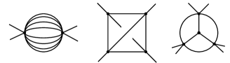
Figure 1: Examples of loop diagrams with no two-particle cuts splitting the graph in two disconnected subgraphs.

We stress-tested our method against current state-of-the-art technology, PLD.jl [18, 20] and HyperInt [46], which utilizes modern algebro-geometric and advanced numerical polynomial solving methods. We found a match with all the examples we tested (see Tab. 1). All of our calculations were performed analytically on a conventional laptop using built-in Mathematica functions.

We also made new predictions for the examples listed in Tab. 2, which existing tools could not solve in useful time. Many of these examples are relevant Standard Model processes involving massive quarks and electroweak bosons. Additionally, we predicted the leading singularity of the $L$-loop pentaladder, which underscores the recursive nature of the method. We emphasize that similar results can be obtained for the general kinematic pentaladder and the $(n>5)$-point ladder. The results are available in the GitHub repository: [48].

In the examples considered here, the system of equations (9) resulted in relatively low-degree polynomial constraints. This might change for more complicated Feynman diagrams, where more refined algebraic geometry methods could be used to compute the discriminant of the system more efficiently. Currently, the complexity and number of polynomial equations are manageable thanks to the recursive nature of the method and the absence of variables other than kinematic invariants. This remains an important technical question to explore further.

A possible conceptual improvement would be to exploit multi-particle cuts. Plausible generalizations of (9) to three-particle cuts could involve replacing $\det\mathcal{G}$ either with a larger Gram determinant that includes the additional intermediate momentum, or with three independent Gram constraints $\det\mathcal{G}(k_{i}\cdot P_{AB}^{\prime})=0$ for each independent cut propagator momentum $k_{i}$ [33, 34]. In practice, this will only become important beyond low loop orders, because the current recursion terminates on two-particle-irreducible diagrams, which can be readily classified; see Fig. 1. The Landau singularities of these diagrams can be determined by other methods such as PLD.jl, which provides a seed to our recursion.

We provided necessary conditions for the existence of complex singularities, which is the important information for many bootstrap applications. Sometimes, it is also necessary to know whether a given singularity can appear on the principal sheet. Since our method in principle constructs momenta (and potentially corresponding Schwinger parameters) that solve the Landau equations, we anticipate that such more refined questions can also be answered recursively.

We anticipate that this work will lead to computational advances in the analytic study of Feynman integrals, including the differential equations bootstrap. We also envision potential applications to other areas of particle physics, e.g., cosmological correlators [49, 50, 51] and inclusive or out-of-time ordered amplitudes [52].

Appendix A Massive pentabox example

The purpose of this section is to demonstrate once more how the method works in practice through a detailed analysis of a known, yet non-trivial, example. We will consider the pentabox with two loops of equal mass $m$

where $p_{i}^{2}=0$ for all $i$. We use the following set of propagators:

$$\begin{aligned} &\mathscr{D}_{1}=(k_{1}{-}p_{23})^{2}{-}m^{2}\,,&&\mathscr{D}_{2}=(k_{1}{-}p_{3})^{2}{-}m^{2}\,,\\ &\mathscr{D}_{3}=k_{1}^{2}{-}m^{2}\,,&&\mathscr{D}_{4}=k_{2}^{2}{-}m^{2}\,,\\ &\mathscr{D}_{5}=(k_{2}{-}p_{4})^{2}{-}m^{2}\,,&&\mathscr{D}_{6}=(k_{2}{+}p_{123})^{2}{-}m^{2}\,,\\ &\mathscr{D}_{7}=(k_{1}{-}p_{123})^{2}{-}m^{2}\,,&&\mathscr{D}_{8}=(k_{2}{+}k_{1})^{2}{-}m^{2}\,.\end{aligned}$$ (22)

The recursion begins with the box (contained in the inner red rectangle) and ends with the full graph (contained in the outer blue rectangle)

(Note that starting with the pentagon yields the same set of singularities in the end, although (9) is harder to solve since it involves one derivative condition.)

For the box, we have the Gram matrix

$$\mathcal{G}_{2}=\Big{[}q_{i}^{(2)}\cdot q_{j}^{(2)}\Big{]}\quad:\leavevmode\nobreak\ q_{\bullet}^{(2)}\in\{p_{4},k_{2},k_{1},p_{123}-k_{1}\}\,.$$ (24)

We can eliminate the internal dot products

$$k_{2}\cdot\{p_{4},k_{2},k_{1},p_{123}-k_{1}\}\,,$$ (25)

by first localizing on the two-particle cut $\mathscr{D}_{4}{=}\mathscr{D}_{6}{=}0$ and then localizing on the leading singular loci $\mathscr{L}(A_{2})_{1}{=}0$ and $\mathscr{L}(B_{2})_{1}{=}0$ of ${A_{2}}$ and ${B_{2}}$, given by $\mathscr{D}_{5}{=}\mathscr{D}_{8}{=}0$. The result is the restricted Gram determinant $\det\tilde{\mathcal{G}}_{2}$ from (8) with $\mathscr{S}=\{\mathscr{L}(A_{2})_{1},\mathscr{L}(B_{2})_{1}\}$, which explicitly reads

$$\footnotesize\begin{vmatrix}0&0&k_{1}{\cdot}p_{4}&p_{4}{\cdot}p_{123}{-}k_{1}{\cdot}p_{4}\\ 0&m^{2}&{-}\frac{k_{1}^{2}}{2}&\frac{k_{1}^{2}{-}p_{123}^{2}}{2}\\ k_{1}{\cdot}p_{4}&{-}\frac{k_{1}^{2}}{2}&k_{1}^{2}&k_{1}\cdot p_{123}{-}k_{1}^{2}\\ p_{4}{\cdot}p_{123}{-}k_{1}{\cdot}p_{4}&\frac{k_{1}^{2}{-}p_{123}^{2}}{2}&k_{1}{\cdot}p_{123}{-}k_{1}^{2}&k_{1}^{2}{+}p_{123}^{2}{-}2k_{1}{\cdot}p_{123}\end{vmatrix}\,.$$ (26)

Setting (26) to zero gives a constraint $(\mathscr{L}(B_{1})_{1}{=}0)$ to impose in the next step of the recursion.

For the full graph, we have the Gram matrix

$$\mathcal{G}_{1}=\Big{[}q_{i}^{(1)}\cdot q_{j}^{(1)}\Big{]}\quad:\leavevmode\nobreak\ q_{\bullet}^{(1)}\in\{p_{3},p_{23},p_{123},k_{1},p_{4}\}\,.$$ (27)

To eliminate all but one internal dot product

$$k_{1}\cdot\{p_{3},p_{23},p_{123},k_{1},p_{4}\}\,,$$ (28)

we first localize on the two-particle cut $\mathscr{D}_{3}{=}\mathscr{D}_{7}{=}0$ and then on the leading singular loci $\mathscr{L}(A_{1})_{1}{=}0$ and $\mathscr{L}(B_{1})_{1}{=}0$ of ${A_{1}}$ and ${B_{1}}$. $\mathscr{L}(A_{1})_{1}{=}0$ is given by $\mathscr{D}_{1}{=}\mathscr{D}_{2}{=}0$, which, together with the two-particle cut, fix $k_{1}^{2}$, $k_{1}\cdot p_{123}$, $k_{1}\cdot p_{3}$ and $k_{1}\cdot p_{23}$. To fix $k_{1}\cdot p_{4}$, we solve $\mathscr{L}(B_{1})_{1}=\eqref{eq:condF1pb}=0$. This yields the restricted Gram determinant $\det\tilde{\mathcal{G}}_{1}$ from (8) with $\mathscr{S}=\{\mathscr{L}(A_{1})_{1},\mathscr{L}(B_{1})_{1}\}$

$$\begin{vmatrix}0&\frac{s_{23}}{2}&\frac{s_{45}{-}s_{12}}{2}&0&\frac{s_{34}}{2}\\ \frac{s_{23}}{2}&s_{23}&\frac{s_{23}{+}s_{45}}{2}&\frac{s_{23}}{2}&\frac{s_{15}{-}s_{23}}{2}\\ \frac{s_{45}{-}s_{12}}{2}&\frac{s_{23}{+}s_{45}}{2}&s_{45}&\frac{s_{45}}{2}&-\frac{s_{45}}{2}\\ 0&\frac{s_{23}}{2}&\frac{s_{45}}{2}&m^{2}&\frac{m^{2}s_{45}^{2}{\pm}2\sigma}{\eta}\\ \frac{s_{34}}{2}&\frac{s_{15}{-}s_{23}}{2}&-\frac{s_{45}}{2}&\frac{m^{2}s_{45}^{2}{\pm}2\sigma}{\eta}&0\end{vmatrix}\,,$$ (29)

where $\sigma=\sqrt{m^{2}s_{45}^{3}(s_{45}-3m^{2})}$ and $\eta=2s_{45}(s_{45}{-}4m^{2})$. Because the result is independent of $k_{1}$, there is no derivative condition to impose and $\mathscr{L}(A_{1}B_{1})_{1}{=}0$ is given by setting $\eqref{eq:finalDetptb}$ equal to zero. The result agrees with D[57] in the database [53], which is one of the leading singularity components flagged by PLD.jl. The other one, D[62], arises from the kinematic normalization $C\propto(\det[p_{i}\cdot p_{j}]_{i,j=1}^{4})^{\frac{5-\mathrm{D}}{2}}$ in (4).

References

- Dixon [2011] L. J. Dixon, Scattering amplitudes: the most perfect microscopic structures in the Universe, J. Phys. A 44, 454001 (2011), arXiv:1105.0771 [hep-th] .
- Bourjaily et al. [2022] J. L. Bourjaily et al., Functions Beyond Multiple Polylogarithms for Precision Collider Physics, in Snowmass 2021 (2022) arXiv:2203.07088 [hep-ph] .
- Weinzierl [2022] S. Weinzierl, Feynman Integrals (2022) arXiv:2201.03593 [hep-th] .
- Drummond et al. [2019] J. Drummond, J. Foster, O. Gürdoğan, and G. Papathanasiou, Cluster adjacency and the four-loop NMHV heptagon, JHEP 03, 087, arXiv:1812.04640 [hep-th] .
- Dixon et al. [2021] L. J. Dixon, A. J. McLeod, and M. Wilhelm, A Three-Point Form Factor Through Five Loops, JHEP 04, 147, arXiv:2012.12286 [hep-th] .
- Caron-Huot et al. [2016] S. Caron-Huot, L. J. Dixon, A. McLeod, and M. von Hippel, Bootstrapping a Five-Loop Amplitude Using Steinmann Relations, Phys. Rev. Lett. 117, 241601 (2016), arXiv:1609.00669 [hep-th] .
- Caron-Huot et al. [2019] S. Caron-Huot, L. J. Dixon, F. Dulat, M. von Hippel, A. J. McLeod, and G. Papathanasiou, Six-Gluon amplitudes in planar = 4 super-Yang-Mills theory at six and seven loops, JHEP 08, 016, arXiv:1903.10890 [hep-th] .
- Dixon and Liu [2020] L. J. Dixon and Y.-T. Liu, Lifting Heptagon Symbols to Functions, JHEP 10, 031, arXiv:2007.12966 [hep-th] .
- Dixon et al. [2022] L. J. Dixon, O. Gurdogan, A. J. McLeod, and M. Wilhelm, Folding Amplitudes into Form Factors: An Antipodal Duality, Phys. Rev. Lett. 128, 111602 (2022), arXiv:2112.06243 [hep-th] .
- Dixon and Liu [2023] L. J. Dixon and Y.-T. Liu, An eight loop amplitude via antipodal duality, JHEP 09, 098, arXiv:2308.08199 [hep-th] .
- Wilhelm and Zhang [2023] M. Wilhelm and C. Zhang, Symbology for elliptic multiple polylogarithms and the symbol prime, JHEP 01, 089, arXiv:2206.08378 [hep-th] .
- Morales et al. [2023] R. Morales, A. Spiering, M. Wilhelm, Q. Yang, and C. Zhang, Bootstrapping Elliptic Feynman Integrals Using Schubert Analysis, Phys. Rev. Lett. 131, 041601 (2023), arXiv:2212.09762 [hep-th] .
- Cao et al. [2023] Q. Cao, S. He, and Y. Tang, Cutting the traintracks: Cauchy, Schubert and Calabi-Yau, JHEP 04, 072, arXiv:2301.07834 [hep-th] .
- He et al. [2023] S. He, X. Jiang, J. Liu, and Q. Yang, On symbology and differential equations of Feynman integrals from Schubert analysis, JHEP 12, 140, [Erratum: JHEP 04, 063 (2024)], arXiv:2309.16441 [hep-th] .
- [15] X. Jiang, J. Liu, X. Xu, and L. L. Yang, Symbol letters of Feynman integrals from Gram determinants, arXiv:2401.07632 [hep-ph] .
- Giroux et al. [2024] M. Giroux, A. Pokraka, F. Porkert, and Y. Sohnle, The soaring kite: a tale of two punctured tori, JHEP 05, 239, arXiv:2401.14307 [hep-th] .
- Landau [1960] L. D. Landau, On analytic properties of vertex parts in quantum field theory, in 9th International Annual Conference on High Energy Physics, Vol. Vol.2 (1960) pp. 95–101.
- [18] C. Fevola, S. Mizera, and S. Telen, Principal Landau Determinants, arXiv:2311.16219 [math-ph] .
- Mizera and Telen [2022] S. Mizera and S. Telen, Landau discriminants, JHEP 08, 200, arXiv:2109.08036 [math-ph] .
- Fevola et al. [2024] C. Fevola, S. Mizera, and S. Telen, Landau Singularities Revisited: Computational Algebraic Geometry for Feynman Integrals, Phys. Rev. Lett. 132, 101601 (2024), arXiv:2311.14669 [hep-th] .
- [21] W. Flieger and W. J. Torres Bobadilla, Landau and leading singularities in arbitrary space-time dimensions, arXiv:2210.09872 [hep-th] .
- Bourjaily et al. [2023] J. L. Bourjaily, C. Vergu, and M. von Hippel, Landau singularities and higher-order polynomial roots, Phys. Rev. D 108, 085021 (2023), arXiv:2208.12765 [hep-th] .
- [23] L. Lippstreu, M. Spradlin, and A. Volovich, Landau Singularities of the 7-Point Ziggurat I, arXiv:2211.16425 [hep-th] .
- Lippstreu et al. [2024] L. Lippstreu, M. Spradlin, A. Yelleshpur Srikant, and A. Volovich, Landau singularities of the 7-point ziggurat. Part II, JHEP 01, 069, arXiv:2305.17069 [hep-th] .
- Klausen [2023] R. P. Klausen, Hypergeometric feynman integrals, Ph.D. thesis, Mainz U. (2023), arXiv:2302.13184 [hep-th] .
- Dlapa et al. [2023] C. Dlapa, M. Helmer, G. Papathanasiou, and F. Tellander, Symbol alphabets from the Landau singular locus, JHEP 10, 161, arXiv:2304.02629 [hep-th] .
- [27] M. Helmer, G. Papathanasiou, and F. Tellander, Landau Singularities from Whitney Stratifications, arXiv:2402.14787 [hep-th] .
- Correia et al. [2022] M. Correia, A. Sever, and A. Zhiboedov, Probing multi-particle unitarity with the Landau equations, SciPost Phys. 13, 062 (2022), arXiv:2111.12100 [hep-th] .
- Mizera [2023] S. Mizera, Natural boundaries for scattering amplitudes, SciPost Phys. 14, 101 (2023), arXiv:2210.11448 [hep-th] .
- [30] M. Berghoff and E. Panzer, Hierarchies in relative Picard-Lefschetz theory, arXiv:2212.06661 [math-ph] .
- Hannesdottir et al. [2023] H. S. Hannesdottir, A. J. McLeod, M. D. Schwartz, and C. Vergu, Constraints on sequential discontinuities from the geometry of on-shell spaces, JHEP 07, 236, arXiv:2211.07633 [hep-th] .
- Mandelstam [1959] S. Mandelstam, Analytic properties of transition amplitudes in perturbation theory, Phys. Rev. 115, 1741 (1959).
- Gribov and Dyatlov [1962] V. N. Gribov and I. T. Dyatlov, Analytic continuation of the three-particle unitarity condition. Simplest diagrams, Sov. Phys. JETP 15, 140 (1962).
- Islam and Kim [1965] J. N. Islam and Y. S. Kim, Analytic property of three-body unitarity integral, Phys. Rev. 138, B1222 (1965).
- Correia et al. [2021] M. Correia, A. Sever, and A. Zhiboedov, An Analytical Toolkit for the S-matrix Bootstrap, JHEP 3, 013, arXiv:2006.08221 [hep-th] .
- [36] M. Correia, Nonperturbative Anomalous Thresholds, arXiv:2212.06157 [hep-th] .
- Tourkine and Zhiboedov [2023] P. Tourkine and A. Zhiboedov, Scattering amplitudes from dispersive iterations of unitarity, JHEP 11, 005, arXiv:2303.08839 [hep-th] .
- Hannesdottir and Mizera [2023] H. S. Hannesdottir and S. Mizera, What is the i for the S-matrix?, SpringerBriefs in Physics (Springer, 2023) arXiv:2204.02988 [hep-th] .
- Cutkosky [1961] R. Cutkosky, Anomalous thresholds, Reviews of Modern Physics 33, 448 (1961).
- Mandelstam [1958] S. Mandelstam, Determination of the pion-nucleon scattering amplitude from dispersion relations and unitarity. general theory, Phys. Rev. 112, 1344 (1958).
- Baikov [1997] P. A. Baikov, Explicit solutions of the multiloop integral recurrence relations and its application, Nucl. Instrum. Meth. A 389, 347 (1997), arXiv:hep-ph/9611449 .
- Mastrolia and Mizera [2019] P. Mastrolia and S. Mizera, Feynman Integrals and Intersection Theory, JHEP 02, 139, arXiv:1810.03818 [hep-th] .
- Coleman and Norton [1965] S. Coleman and R. E. Norton, Singularities in the physical region, Nuovo Cim. 38, 438 (1965).
- Hwa and Teplitz [1966] R. Hwa and V. Teplitz, Homology and Feynman Integrals, Mathematical physics monograph series (W. A. Benjamin, 1966).
- dat [2023a] https://mathrepo.mis.mpg.de/_downloads/aee2fc92131df00a43a9ede2781a5043/par_generic_generic.txt (2023a), accessed: 2024-06-04.
- Panzer [2015] E. Panzer, Algorithms for the symbolic integration of hyperlogarithms with applications to Feynman integrals, Comput. Phys. Commun. 188, 148 (2015), arXiv:1403.3385 [hep-th] .
- Klemm et al. [2020] A. Klemm, C. Nega, and R. Safari, The -loop Banana Amplitude from GKZ Systems and relative Calabi-Yau Periods, JHEP 04, 088, arXiv:1912.06201 [hep-th] .
- rep [2024] github.com/StrangeQuark007/recursive_landau (2024), accessed: 2024-06-04.
- Weinberg [2005] S. Weinberg, Quantum contributions to cosmological correlations, Phys. Rev. D 72, 043514 (2005), arXiv:hep-th/0506236 .
- [50] N. Arkani-Hamed, D. Baumann, A. Hillman, A. Joyce, H. Lee, and G. L. Pimentel, Differential Equations for Cosmological Correlators, arXiv:2312.05303 [hep-th] .
- Baumann et al. [2022] D. Baumann, D. Green, A. Joyce, E. Pajer, G. L. Pimentel, C. Sleight, and M. Taronna, Snowmass White Paper: The Cosmological Bootstrap, in Snowmass 2021 (2022) arXiv:2203.08121 [hep-th] .
- Caron-Huot et al. [2024] S. Caron-Huot, M. Giroux, H. S. Hannesdottir, and S. Mizera, What can be measured asymptotically?, JHEP 01, 139, arXiv:2308.02125 [hep-th] .
- dat [2023b] https://mathrepo.mis.mpg.de/_downloads/26c5735446b8f1a7b28e61527c1eab05/pentb_equal_zero.txt (2023b), accessed: 2024-06-04.