Quantitative convergence guarantees for the mean-field dispersion process

Abstract

We study the dispersion process on the complete graph introduced in the recent work [19] under the mean-field framework. In contrast to the probabilistic approach taken in [19] and many other related works, our focus is on the investigation of the large time behavior of solutions of the associated kinetic mean-field system of nonlinear ordinary differential equations (ODEs). We establish various analytical and quantitative convergence results for the long time behaviour of the mean-field system and related numerical illustrations are also provided.

Key words: Dispersion of particles; Agent-based model; Interacting particle systems; Fokker–Planck equations; Econophysics

1 Introduction

We study the so-called dispersion process on the complete graph with $N$ vertices (denoted by $G_{N}$) introduced by Cooper, McDowell, Radzik, Rivera and Shiraga [17] and investigated in many subsequent works [19, 24, 37]. The dispersion process proposed in [17, 19] can be described as follows: Initially, $M\in\mathbb{N}_{+}$ indistinguishable particles are placed on a single vertex of $G_{N}$. At the beginning of each time step, for every vertex occupied by at least two particles, each of these particles moves independently to another vertex on $G_{N}$ chosen uniformly at random. It is easy to convince us that the aforementioned process will freeze at the first time when each vertex hosts at most one particle, if $M\leq N$.

In this manuscript, we will investigate a continuous-time version of the aforementioned dispersion model by virtue of the tools from kinetic theory. To fix notations throughout the rest the paper, we will label the vertex set of $G_{N}$ from $1$ to $N$ and denote by $X_{i}(t)$ the number of particles inhabiting vertex $i$ at time $t\in\mathbb{R}_{+}$, and set

$$X(t)=\left(X_{1}(t),\ldots,X_{N}(t)\right)$$

to be the state vector of the dynamics. The state space is thus

$$\Omega=\{X\in\mathbb{N}^{N}\mid X_{1}+\cdots+X_{N}=M\}.$$ (1.1)

The continuous-time analog of the dispersion model suggested in [17, 19] is dictated by the following dynamics: at random times (generalized by exponential law), each non-empty vertex $i$ which is inhabited by at least two particles expels a particle at the rate $X_{i}$ to another uniformly chosen vertex $j$. We illustrate our model via Figure 1 below.

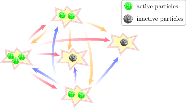
Figure 1: Illustration of the dispersion dynamics on a complete graph with $N=5$ nodes/sites and $M=9$ particles. Particles which share a common site will be “active” and move across sites.

Employing the terminology introduced in [19], a particle will be called happy if it does not occupy the same site with other particles, otherwise it is unhappy. Consequently, in the dispersion process on the complete graph, only unhappy (or “active”) particles have the motivation to move to a different site.

Remark. It is also possible to interpret the dispersion process using terminologies from econophysics (which is a sub-branch of statistical physics that apply concepts and techniques of traditional physics to economics and finance [20, 15, 21, 28, 35, 36]). Indeed, if we think of particles as dollars, vertices as agents, and $X_{i}(t)$ as the amount of dollars agent $i$ has at time $t$, then the aforementioned dispersion process can be viewed as the following simple dollar exchange mechanism in a closed economical system: at random times (generated by an exponential law), an agent $i$ who has at least two dollars in his/her pocket (i.e., $X_{i}\geq 2$) is picked at a rate proportional to his/her fortune $X_{i}$, then he or she will give one dollar to another agent $j$ picked uniformly at random. It is clearly from the set-up that we have

$$X_{1}(t)+\cdots+X_{N}(t)=N\mu=M\qquad\text{for all }t\geq 0$$ (1.2)

since the economical system is closed, where $\mu\coloneqq M/N$ denotes the average amount of dollars per agent in this context. Mathematically, the update rule of this multi-agent system can be represented by

$$\textbf{Dispersion process:}\qquad(X_{i},X_{j})~{}\leavevmode\hbox to18.47pt{\vbox to16.28pt{\text{[drawing]}}}~{}(X_{i}-1,X_{j}+1)\quad(\text{if }X_{i}>1). X_{i} X_{i}$$ (1.3)

It is worth noting that the model (1.3) resembles the so-called poor-biased exchange model in econophysics [7, 13] in which one replaces the update rule (1.3) by the following:

$$\textbf{Poor-biased exchange:}\qquad(X_{i},X_{j})~{}\leavevmode\hbox to17.47pt{\vbox to16.02pt{\text{[drawing]}}}~{}(X_{i}-1,X_{j}+1). X_{i} X_{i}$$ (1.4)

Therefore, one can view the dispersion process as a modified dynamics of the poor-biased exchange model (1.4) with the inclusion of a wealth-flooring policy, which prevents agents whose wealth are no more than $1$ dollar from giving out their dollars to other agents.

We emphasize that earlier works on the dispersion process on complete graphs [19] focuses only on the asymptotic region where the total number of particles $M$ scales no faster than the total number of sites $N$ (i.e., $\lim_{N\to\infty}=M/N\leq 1$). In this regime, the process ends almost surely when no particle is sharing the same site with other particles, and every particle becomes happy at the (random) time $T_{G_{N},M}$ termed as the dispersion time. The main quantity under investigation in [17, 19, 24, 37] is the aforementioned dispersion time via advanced probabilistic tools. By resorting to a kinetic/mean-field approach, we aim to treat the case where $\mu=M/N\in(0,\infty)$ remains a positive constant of order $1$ and we also allow for general initial distributions of particles beyond the common choice of putting all particles on a single site.

To foresee the behavior of the dynamics under the large time and the large population limits, we perform agent-based simulations using $N=1,000$ after $2000$ time units using two different values for $\mu$ (see Figure 2). We observe that the distribution of the number of particles in a site converges to a Bernoulli distribution with mean $0.8$ for $\mu=0.8$ (Figure 3-left) and that it stabilizes near a zero-truncated Poisson distribution with mean $2$ predicated by (1.10) for $\mu=2$ (Figure 3-right).

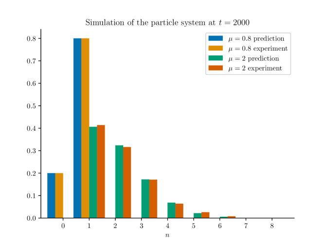
Figure 2: Distribution of particles for the dispersion model with $N=1,000$ agents after $2,000$ units of time, using two different values of $\mu$. For $\mu=0.8$, the final distribution coincides exactly with the Bernoulli distribution with mean $0.8$, where we put all the particles into a single site initially. For $\mu=2$, the terminal distribution is well-approximated by a zero-truncated Poisson distribution prescribed by (1.10) below, where we put $X_{i}(0)=\mu$ for all $1\leq i\leq N$ initially.

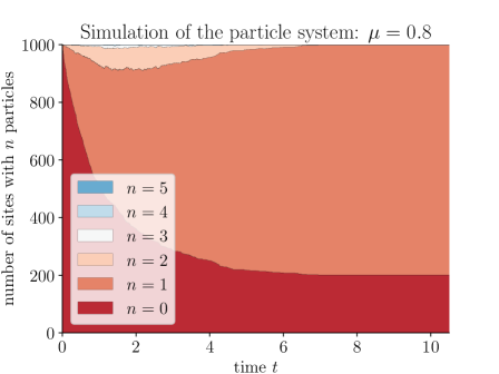
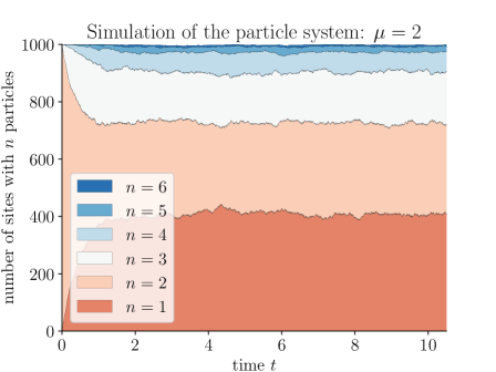
Figure 3: Stackplots of the agent-based simulation with $\mu=0.8$ and $\mu=2$ during the first $10$ units of time. At a given time $t$, the width of $n$-th layer represents the number of sites hosting $n$ particles, making a total of $N=1,000$ sites. For $\mu=0.8$, we initially put all particles at one single site; the distribution of particles converges to a Bernoulli distribution and no site hosts two or more particles (left). For $\mu=2$, we put two particles in each site initially; each site hosts at least one particle and the distribution of particles stabilizes around a zero-truncated Poisson distribution after a few units of time (right).

The continuous-time dispersion model we have described is a standard interacting particle system and is amenable to mean-field type analysis under the large population limit $N\to\infty$, which is detailed in a recent work [11] on a related model. In order to carry out the mean-field analysis as $N\to\infty$, the concept of propagation of chaos [38] plays a crucial role. Bearing in mind our aim to obtain a simplified (and fully deterministic) dynamics when we send $N\to\infty$, we consider the probability distribution function of particles:

$${\bf p}(t)=\left(p_{0}(t),p_{1}(t),\ldots,p_{n}(t),\ldots\right)$$ (1.5)

with $p_{n}(t)=\{``\text{probability that a typical site has }n\text{ particles at time}~{}t"\}$. It has been indicated in a very recent work [11] that evolution of ${\bf p}(t)$ is governed by the following deterministic system of nonlinear ordinary differential equations:

$$\frac{\mathrm{d}}{\mathrm{d}t}{\bf p}(t)=\mathcal{L}[{\bf p}(t)]$$ (1.6)

with

$$\mathcal{L}[{\bf p}]_{n}=\begin{cases}-\left(\sum_{k\geq 2}k\,p_{k}\right)\,p_{0}&n=0,\\ 2\,p_{2}+\left(\sum_{k\geq 2}k\,p_{k}\right)\,p_{0}-\left(\sum_{k\geq 2}k\,p_{k}\right)\,p_{1}&n=1,\\ (n+1)\,p_{n+1}+\left(\sum_{k\geq 2}k\,p_{k}\right)\,p_{n-1}-\left(n+\sum_{k\geq 2}k\,p_{k}\right)\,p_{n}&n\geq 2.\end{cases}$$ (1.7)

The rigorous justification of this transition from the stochastic interacting agents systems (1.3) into the associated mean-field ODE system (1.6)-(1.7) requires the proof of the propagation of chaos property [38], which is beyond the scope of the present manuscript. On the other hand, propagation of chaos property has been proved for other econophysics models, see for instance [7, 8, 9, 10, 13, 18] and we also refer interested readers to [4, 5, 6, 12, 14, 16, 26, 30, 31, 32] for many other interesting models in econophysics literature that we omit to describe in details.

Once the mean-field system of ODEs (1.6)-(1.7) associated to the interacting particle system has been identified, one natural follow-up step is to investigate the long time behaviour of the infinite dimensional ODE system (1.6)-(1.7) with the hope of showing convergence of its solution towards an equilibrium distribution, and we take on this task in the following sections. As will be shown in Section 2, the large time asymptotic of the solution to (1.6)-(1.7) depends on the value of the parameter $\mu\in(0,\infty)$ which represents the average amount of particles per site initially. We prove in Section 3 via the construction of a appropriate Lyapunov functional that solutions of (1.6)-(1.7) converges to the following Bernoulli distribution ${\bf p}^{*}=\left(p^{*}_{0},p^{*}_{1},\ldots,p^{*}_{n},\ldots\right)$

$$p^{*}_{0}=1-\mu,\quad p^{*}_{1}=\mu,\quad p^{*}_{n}=0\quad\text{for }n\geq 2$$ (1.8)

when $\mu\in(0,1]$. Note in particular that the two-point Bernoulli distribution (1.8) boils down to the Dirac delta distribution $\delta_{1}$ centered at $1$, defined via

$$\delta_{1}=(0,1,0,\ldots,0,\ldots),$$ (1.9)

when $\mu=1$. We demonstrate in Section 4 the convergence of solutions of (1.6)-(1.7) to the following zero-truncated Poisson distribution $\mkern 1.5mu\overline{\mkern-1.5mu{\bf p}\mkern-1.5mu}\mkern 1.5mu=\left(\mkern 1.5mu\overline{\mkern-1.5mup\mkern-1.5mu}\mkern 1.5mu_{0},\mkern 1.5mu\overline{\mkern-1.5mup\mkern-1.5mu}\mkern 1.5mu_{1},\ldots,\mkern 1.5mu\overline{\mkern-1.5mup\mkern-1.5mu}\mkern 1.5mu_{n},\ldots\right)$ (in various senses) when $\mu>1$:

$$\mkern 1.5mu\overline{\mkern-1.5mup\mkern-1.5mu}\mkern 1.5mu_{0}=0,\quad\mkern 1.5mu\overline{\mkern-1.5mup\mkern-1.5mu}\mkern 1.5mu_{n}=\frac{\nu^{n}}{n!}\cdot\frac{1}{\mathrm{e}^{\nu}-1}\,\quad\text{for }n\geq 1$$ (1.10)

where $\nu=\mu+W_{0}\left(-\mu\,\mathrm{e}^{-\mu}\right)$ and $W_{0}(\cdot)$ denotes the principal branch of the Lambert $W$ function [29].

We remark here that the mathematical analysis of the large time behavior of the system (1.6)-(1.7) is much trickier when $\mu>1$. Instead of finding a Lyapunov function, we analyze the long time behavior of the probability generating function (PGF), which satisfies a transport equation. We deduce convergence to the zero-truncated Poisson distribution at exponential rate by establishing pointwise convergence of the PGF.

The main result is summarized in the following theorem, which combines Corollary 3.2 and Corollary 4.11.

Theorem 1

There exists a positive constant $C$ depending only on $\mu$ and ${\bf p}(0)$, such that any solution ${\bf p}(t)$ to (1.6)-(1.7) with finite initial variance converges strongly to its equilibrium distribution as $t\to+\infty$. To be precise, denote $\nu\coloneqq\mu+W_{0}(-\mu\mathrm{e}^{-\mu})\in(\mu-1,\mu)$ for $\mu>1$ and $\langle t\rangle\coloneqq\sqrt{1+t^{2}}$ for $t\geq 0$, we have:

1. If $0<\mu<1$, then

   $$\|{\bf p}(t)-{\bf p}^{*}\|_{\ell^{1}}\leq C\,\mathrm{e}^{-2\,(1-\mu)\,t}.$$

2. If $\mu=1$, then

   $$\|{\bf p}(t)-{\bf p}^{*}\|_{\ell^{1}}\leq C\,t^{-1}.$$

3. If $1<\mu<1+\frac{1}{\mathrm{e}-1}$, then

   $$\left\lVert{\bf p}(t)-\mkern 1.5mu\overline{\mkern-1.5mu\bf p\mkern-1.5mu}\mkern 1.5mu\right\rVert_{\ell^{1}}\leq C\,\langle t\rangle^{\frac{1}{2}}\,\mathrm{e}^{-\nu t}.$$

4. If $\mu\geq 1+\frac{1}{\mathrm{e}-1}$, then there exists $N>0$ depending only on $\mu$ such that

   $$\left\lVert{\bf p}(t)-\mkern 1.5mu\overline{\mkern-1.5mu\bf p\mkern-1.5mu}\mkern 1.5mu\right\rVert_{\ell^{1}}\leq C\,\langle t\rangle^{N+\frac{1}{2}}\,\mathrm{e}^{-t}.$$

2 Elementary properties of the ODE system

After we achieved the transition from the interacting agents system (1.3) to the deterministic nonlinear ODE system (1.6)-(1.7), our main goal is to show convergence of solution of (1.6)-(1.7) to its (unique) equilibrium solution. We aim to describe some elementary properties of solutions of (1.6)-(1.7) in this section. As we have indicated in the introduction, the large time behavior of solutions to (1.6)-(1.7) depends critically on the range to which the parameter $\mu$ belongs. Before we dive into the detailed analysis of the system of nonlinear ODEs, we first establish some preliminary observations regarding solutions of (1.6)-(1.7).

Lemma 2.1

If ${\bf p}(t)$ is a solution to the system (1.6)-(1.7), then

$$\sum_{n=0}^{\infty}\mathcal{L}[{\bf p}]_{n}=0\quad\text{and}\quad\sum_{n=0}^{\infty}n\,\mathcal{L}[{\bf p}]_{n}=0.$$ (2.1)

In particular, the total probability mass and the average amount of particles per site are conserved.

The proof of Lemma 2.1 is based on straightforward computations and will be skipped. Thanks to these conservation relations, the solution ${\bf p}(t)$ lives in the space of probability distributions on $\mathbb{N}$ with the prescribed mean value $\mu$, defined by

$$\mathcal{S}_{\mu}\coloneqq\left\{{\bf p}\in[0,1]^{\mathbb{N}}\Bigm{|}\sum_{n=0}^{\infty}p_{n}=1,~{}\sum_{n=0}^{\infty}n\,p_{n}=\mu\right\}.$$ (2.2)

More importantly, the system (1.6)-(1.7) will be equivalent to the following system of nonlinear ODEs:

$$\frac{\mathrm{d}}{\mathrm{d}t}{\bf p}(t)=\mathcal{L}[{\bf p}(t)]$$ (2.3)

in which

$$\mathcal{L}[{\bf p}]_{n}=\begin{cases}-\left(\mu-p_{1}\right)\,p_{0}&n=0,\\ 2\,p_{2}+\left(\mu-p_{1}\right)\,p_{0}-\left(\mu-p_{1}\right)\,p_{1}&n=1,\\ (n+1)\,p_{n+1}+\left(\mu-p_{1}\right)\,p_{n-1}-\left(n+\mu-p_{1}\right)\,p_{n}&n\geq 2.\end{cases}$$ (2.4)

Remark. The Fokker–Planck type equation (2.3)-(2.4) admits a heuristic interpretation as a jump process with loss and gain, and we illustrate this perspective via Figure 4 below. We also recall that $\mu-p_{1}(t)$ represents the proportion of unhappy particles at time $t$.

Figure 4: Schematic illustration of the Fokker–Planck type system of nonlinear ODEs (2.3)-(2.4) as a jump process with loss and gain.

Remark. The system (2.3)-(2.4) also resembles another system of nonlinear ODEs known as the Becker-Döring cluster equations. For both systems, the generator $\mathcal{L}$ is a second-order difference operator linear in $\{p_{2},p_{3},\dots,\}$ but is nonlinear in $p_{1}$. We refer interested readers to [1, 3, 2, 27, 33, 34] and references therein.

Next, we identify the unique equilibrium solution associated with the system (2.3)-(2.4).

Proposition 2.2

The unique equilibrium solution of (2.3)-(2.4) in the space $\mathcal{S}_{\mu}$, for $\mu\in(0,1]$, is given by $\bf p^{*}$ defined in (1.8). The unique equilibrium solution of (2.3)-(2.4) in the space $\mathcal{S}_{\mu}$, when $\mu\in(1,\infty)$, is provided by $\mkern 1.5mu\overline{\mkern-1.5mu{\bf p}\mkern-1.5mu}\mkern 1.5mu$ defined in (1.10).

Proof.

From the evolution equation defined by (2.3)-(2.4), it is straightforward to check that

$$n\,p_{n}=(\mu-p_{1})\,p_{n-1}\quad\forall~{}n\geq 2,\quad\text{and}\quad(\mu-p_{1})\,p_{0}=0$$ (2.5)

must hold at equilibrium. On the one hand, if $\mu=p_{1}\leq 1$, then $p_{n}=0$ for all $n\geq 2$, and we deduce that the unique equilibrium solution, denoted by ${\bf p}^{*}$, is

$$p^{*}_{0}=1-\mu,\quad p^{*}_{1}=\mu,\quad p^{*}_{n}=0\quad\text{for }n\geq 2.$$

On the other hand, for $\mu>1\geq p_{1}$, we deduce from (2.5) that $p_{0}=0$, and the unique equilibrium distribution, denoted by $\mkern 1.5mu\overline{\mkern-1.5mu{\bf p}\mkern-1.5mu}\mkern 1.5mu$, is

$$\mkern 1.5mu\overline{\mkern-1.5mup\mkern-1.5mu}\mkern 1.5mu_{0}=0,\quad\mkern 1.5mu\overline{\mkern-1.5mup\mkern-1.5mu}\mkern 1.5mu_{n}=\frac{(\mu-\mkern 1.5mu\overline{\mkern-1.5mup\mkern-1.5mu}\mkern 1.5mu_{1})^{n-1}}{n!}\,\mkern 1.5mu\overline{\mkern-1.5mup\mkern-1.5mu}\mkern 1.5mu_{1}\quad\text{for }n\geq 1$$ (2.6)

where $\mkern 1.5mu\overline{\mkern-1.5mup\mkern-1.5mu}\mkern 1.5mu_{1}>0$ is chosen such that $\mkern 1.5mu\overline{\mkern-1.5mu{\bf p}\mkern-1.5mu}\mkern 1.5mu\in\mathcal{S}_{\mu}$. Since $\sum_{n\geq 0}\mkern 1.5mu\overline{\mkern-1.5mup\mkern-1.5mu}\mkern 1.5mu_{n}=1$, we deduce that $\mkern 1.5mu\overline{\mkern-1.5mup\mkern-1.5mu}\mkern 1.5mu_{1}\,\mathrm{e}^{-\mkern 1.5mu\overline{\mkern-1.5mup\mkern-1.5mu}\mkern 1.5mu_{1}}=\mu\,\mathrm{e}^{-\mu}$, whence $\mkern 1.5mu\overline{\mkern-1.5mup\mkern-1.5mu}\mkern 1.5mu_{1}=-W_{0}\left(-\mu\,\mathrm{e}^{-\mu}\right)$. We finish the proof by introducing a new constant $\nu=\mu-\bar{p}_{1}$. $\square$

Remark. The zero-truncated Poisson distribution $\mkern 1.5mu\overline{\mkern-1.5mu{\bf p}\mkern-1.5mu}\mkern 1.5mu$ defined in (1.10) admits a simple interpretation in terms of random variables. Indeed, if $X\sim\textrm{Possion}\left(\nu\right)$, then the distribution of $X$ conditioned on $X\geq 1$ obeys the zero-truncated Poisson distribution, whose law is given by $\mkern 1.5mu\overline{\mkern-1.5mu{\bf p}\mkern-1.5mu}\mkern 1.5mu$.

As a warm-up before we dive into the analytical investigation of the nonlinear ODE system (2.3)-(2.4) in the upcoming sections, we investigate numerically the convergence of ${\bf p}(t)$ to its equilibrium distribution. We use $\mu=2$ and $\mu=0.8$ respectively. To discretize the model, we use $101$ components to describe the distribution ${\bf p}(t)$ (i.e., $(p_{0}(t),\ldots,p_{100}(t))$). As initial condition, we use $p_{100}(0)=\frac{\mu}{100}$, $p_{0}(0)=1-p_{100}(0)$ and $p_{i}(0)=0$ for $i\notin\{0,100\}$. The standard Runge-Kutta fourth-order scheme is used to discretize the ODE system (2.3)-(2.4) with the time step $\Delta t=0.01$. We plot in Figure 5 the evolution of the numerical solution ${\bf p}(t)$ at different times corresponding to $\mu=0.8$ and $\mu=2$, respectively. It can be observed that convergence to equilibrium occur in both cases.

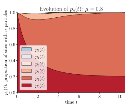
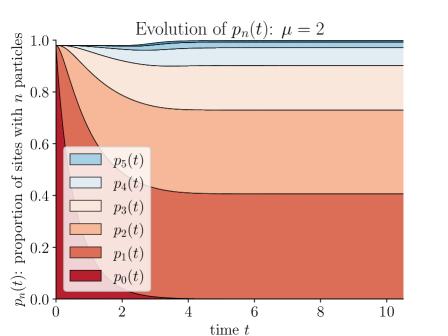
Figure 5: Stackplot of the numerical solution to the truncated ODE system $\{p_{n}(t)\}_{n=0}^{100}$ with $\mu=0.8$ and $\mu=2$ during the first 10 units of time. At a given time $t$, the width of $n$-th layer represents $p_{n}(t)$ which sum up to $1$. For $\mu=0.8$ the distibution of particles converges to a Bernoulli distribution with mean $\mu$ (left). For $\mu=2$, the distribution converges to the zero-truncated Poisson distribution with mean $\mu$ (right).

3 Convergence to Bernoulli distribution for $\mu\leq 1$

To justify the large time convergence of solutions of the system (2.3)-(2.4) when $\mu\in(0,1]$, we employ a suitable Lyapunov functional associated to the dynamics (2.3)-(2.4). For this purpose, we define the following energy functional:

$$\mathcal{E}[{\bf p}]=\sum_{n\geq 0}n^{2}\,p_{n}-\mu$$ (3.1)

for each ${\bf p}\in\mathcal{S}_{\mu}$, which is just a shifted version of the second (raw) moment of the distribution ${\bf p}$. We first start with an elementary variational characterization of the Bernoulli distribution ${\bf p}^{*}$.

Lemma 3.1

For each $\mu\in(0,1]$, the Bernoulli distribution ${\bf p}^{*}$ with parameter $\mu$ satisfies

$${\bf p}^{*}=\operatorname*{\arg\!\min}\limits_{{\bf p}\in\mathcal{S}_{\mu}}\sum_{n\geq 0}n^{2}\,p_{n}.$$ (3.2)

Consequently, $\mathcal{E}[{\bf p}]\geq 0$ for all ${\bf p}\in\mathcal{S}_{\mu}$ and the equality holds if and only if ${\bf p}={\bf p}^{*}$.

Proof.

Since ${\bf p}\in\mathcal{S}_{\mu}$, we have $\sum_{n\geq 0}n\,p_{n}=\mu$ and thus $\sum_{n\geq 1}n^{2}\,p_{n}\geq\sum_{n\geq 1}n\,p_{n}=\mu$, in which the inequality will become an equality if and only if $p_{n}=0$ for all $n\geq 2$. This finishes the proof of Lemma 3.1. $\square$

We now prove the following quantitative convergence result for the dissipation of $\mathcal{E}[{\bf p}(t)]$ along solutions to the system of nonlinear ODEs (2.3)-(2.4) when $\mu\in(0,1]$.

Theorem 2

Assume that ${\bf p}(t)$ is the classical solution to the system (2.3)-(2.4) with ${\bf p}(0)\in\mathcal{S}_{\mu}$ and $\mu\in(0,1]$, then for all $t\geq 0$ we have

$$\mathcal{E}[{\bf p}(t)]\leq\mathcal{E}[{\bf p}(0)]\,\mathrm{e}^{-2\,(1-\mu)\,t}~{}~{}\text{when~{} $\mu<1$}$$ (3.3)

and

$$\mathcal{E}[{\bf p}(t)]\leq\mathcal{E}[{\bf p}(0)]\,\mathrm{e}^{-2\,t}+\frac{4}{t+2/p_{0}(0)}+2\,p_{0}(0)\,\mathrm{e}^{-t}~{}~{}\text{when~{} $\mu=1$}.$$ (3.4)

Proof.

A straightforward computation gives us

$$\frac{\mathrm{d}}{\mathrm{d}t}\mathcal{E}[{\bf p}] =2\,p_{2}+(\mu-p_{1})\,(p_{0}-p_{1})$$ (3.5)

$$\qquad+\sum_{n\geq 2}n^{2}\,\left[(n+1)\,p_{n+1}-n\,p_{n}-(\mu-p_{1})\,(p_{n}-p_{n-1})\right]$$

$$=2\,p_{2}+(\mu-p_{1})\,(p_{0}-p_{1})$$

$$\qquad+\sum_{n\geq 2}\left[n^{2}\,(n+1)\,p_{n+1}-n^{3}\,p_{n}\right]-(\mu-p_{1})\,\sum_{n\geq 2}n^{2}\,(p_{n}-p_{n-1})$$

$$=2\,p_{2}+(\mu-p_{1})\,(p_{0}-p_{1})$$

$$\qquad+\left(p_{1}-2\,p_{2}+\mu-2\,\sum_{n\geq 0}n^{2}\,p_{n}\right)-(\mu-p_{1})\,(p_{0}-p_{1}-1-2\,\mu)$$

$$=p_{1}+\mu-2\,\sum_{n\geq 0}n^{2}\,p_{n}+(\mu-p_{1})\,(1+2\,\mu)$$

$$=-2\,\mathcal{E}[{\bf p}]+2\,\mu\,(\mu-p_{1}).$$

We observe that $0\leq\mu-p_{1}=\sum_{n\geq 2}n\,p_{n}\leq\sum_{n\geq 2}(n^{2}-n)\,p_{n}=\mathcal{E}[{\bf p}]$ for all ${\bf p}\in\mathcal{S}_{\mu}$, thus for $\mu\in(0,1)$ we deduce from (3.5) that

$$\frac{\mathrm{d}}{\mathrm{d}t}\mathcal{E}[{\bf p}]\leq-(2-2\,\mu)\,\mathcal{E}[{\bf p}],$$

from which the exponential decay of $\mathcal{E}[{\bf p}(t)]$ (3.3) follows immediately. On the other hand, for $\mu=1$, we have $2\,p_{0}+p_{1}\geq 1$ since ${\bf p}\in\mathcal{S}_{1}$. The differential equation satisfied by $p_{0}$ implies that $p^{\prime}_{0}=-(1-p_{1})\,p_{0}\leq-p^{2}_{0}$, whence

$$p_{0}(t)\leq\frac{1}{t+1/p_{0}(0)}~{}~{}\text{and}~{}~{}p_{1}(t)\geq 1-\frac{2}{t+1/p_{0}(0)}$$

for all $t\geq 0$. Consequently, we derive from (3.5) the following differential inequality:

$$\frac{\mathrm{d}}{\mathrm{d}t}\mathcal{E}[{\bf p}]\leq-2\,\mathcal{E}[{\bf p}]+\frac{4}{t+1/p_{0}(0)},$$

whence

$$\mathcal{E}[{\bf p}(t)]\leq\mathcal{E}[{\bf p}(0)]\,\mathrm{e}^{-2\,t}+4\,\mathrm{e}^{-2\,t}\,\int_{0}^{t}\frac{\mathrm{e}^{2\,s}}{s+1/p_{0}(0)}\,\mathrm{d}s.$$ (3.6)

To conclude the proof and reach the advertised upper bound (3.4), it suffices to notice that

$$\int_{0}^{t}\frac{\mathrm{e}^{2\,s}}{s+1/p_{0}(0)}\,\mathrm{d}s =\int_{0}^{\frac{t}{2}}\frac{\mathrm{e}^{2\,s}}{s+1/p_{0}(0)}\,\mathrm{d}s+\int_{\frac{t}{2}}^{t}\frac{\mathrm{e}^{2\,s}}{s+1/p_{0}(0)}\,\mathrm{d}s$$

$$\leq p_{0}(0)\,\int_{0}^{\frac{t}{2}}\mathrm{e}^{2\,s}\,\mathrm{d}s+\frac{1}{\frac{t}{2}+\frac{1}{p_{0}(0)}}\,\int_{\frac{t}{2}}^{t}\mathrm{e}^{2\,s}\,\mathrm{d}s$$

$$\leq\frac{1}{2}\,p_{0}(0)\,\mathrm{e}^{t}+\frac{\mathrm{e}^{2\,t}}{t+2/p_{0}(0)}$$

for all $t\geq 0$. Thus the proof of Theorem 2 is completed. $\square$

To illustrate the decay of the energy $\mathcal{E}$ numerically, we use the same set-up as in the previous experiment shown in Figure 6 for two different values of $\mu\in(0,1]$, using the semi-log scale.

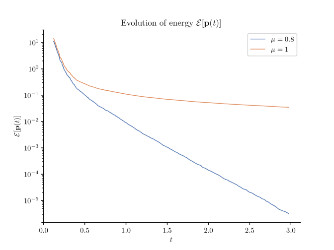
Figure 6: Evolution of the energy $\mathcal{E}[{\bf p}(t)]$ over $0\leq t\leq 3$ with $\mu=0.8$ and $\mu=1$. It can be seen from the picture that the energy decays exponentially for $\mu=0.8$ with rate $C\,\mathrm{e}^{-0.4t}$. For $\mu=1$ the decay is slower.

As an immediate corollary, we can readily deduce the following strong convergence in $\ell^{1}$.

Corollary 3.2

Under the settings of Theorem 2, if ${\bf p}(0)$ has a finite variance, then there exists some constant $C>0$ depending only on $\mu$ and the initial datum ${\bf p}(0)$ such that for all $t>0$, it holds that

$$\|{\bf p}(t)-{\bf p}^{*}\|_{\ell^{1}}\leq C\,\mathrm{e}^{-2\,(1-\mu)\,t}~{}~{}\text{when~{} $\mu<1$}$$ (3.7)

and

$$\|{\bf p}(t)-{\bf p}^{*}\|_{\ell^{1}}\leq\frac{C}{t}~{}~{}\text{when~{} $\mu=1$}.$$ (3.8)

Proof.

We only prove the bound (3.8) when $\mu=1$ as the other bound (3.7) which is valid for $\mu\in(0,1)$ can be handled in a pretty similar way. Notice that

$$\mathcal{E}[{\bf p}(t)]=\sum_{n\geq 0}n^{2}\,p_{n}(t)-1=\sum_{n\geq 0}(n^{2}-n)\,p_{n}(t)=\sum_{n\geq 2}(n^{2}-n)\,p_{n}(t)$$

and $n^{2}\leq 2(n^{2}-n)$ for all $n\geq 2$, hence $\sum_{n\geq 2}n^{2}\,p_{n}(t)\leq 2\,\mathcal{E}[{\bf p}(t)]$. Therefore, we deduce that

$$\|{\bf p}(t)-{\bf p}^{*}\|_{\ell^{1}} =p_{0}(t)+1-p_{1}(t)+\sum_{n\geq 2}p_{n}(t)=2\,(1-p_{1}(t))$$

$$=2\,\left(\sum_{n\geq 2}n^{2}\,p_{n}(t)-\mathcal{E}[{\bf p}(t)]\right)\leq 2\,\mathcal{E}[{\bf p}(t)]\leq\frac{C}{t}$$

for some constant $C>0$ depending on ${\bf p}(0)$ and $\mu$. $\square$

4 Relaxation to zero-truncated Poisson distribution for $\mu>1$

We use a different approach to study the system (2.3)-(2.4) when $\mu>1$. Treating $p_{1}$ as a known function, we first show that the probability generating function solves a first order partial differential equation (PDE), which turns out to be an explicitly solvable transport equation. By writing out the solution, we show that an auxiliary function

$$v(t)\coloneqq\exp\left(\int_{0}^{t}\mathrm{e}^{-t+s}\,(\mu-p_{1}(s))\,\mathrm{d}s\right)$$ (4.1)

must satisfy a nonlinear Volterra-type integral equation [25]. We then study this integral equation to extract convergence and convergence rate, which further sheds light on the convergence of the distribution ${\bf p}(t)$ to the zero-truncated Poisson distribution $\mkern 1.5mu\overline{\mkern-1.5mu{\bf p}\mkern-1.5mu}\mkern 1.5mu$ (1.10).

4.1 Probability generating function

Define the probability generating function $G:[0,+\infty)\times[-1,1]$ of the solution ${\bf p}(t)$ to (2.3)-(2.4) by

$$G(t,z)=\sum_{n=0}^{\infty}p_{n}(t)\,z^{n}.$$

Since $p_{n}(t)\geq 0$ and $\sum_{n=0}^{\infty}p_{n}(t)=1$, we know the above series is absolutely summable. Moreover, because $\sum_{n=0}^{\infty}np_{n}(t)=\mu$, we know that

$$\frac{\partial G}{\partial z}(t,z)=\sum_{n=1}^{\infty}n\,p_{n}(t)\,z^{n-1}$$

is absolutely summable. The ODE system (2.3)-(2.4) can thus be written as the following PDE for $G$:

$$\partial_{t}G =(1-z)[\partial_{z}G-(\mu-p_{1}(t))G-p_{1}(t)].$$ (4.2)

We also recall that the probability generating function can recover the following statistics:

$$\dfrac{\partial^{k}}{\partial z^{k}}G(t,0)=k!\,p_{k}(t)$$

$$\dfrac{\partial^{k}}{\partial z^{k}}G(t,1)=\sum_{n=0}^{\infty}n\,(n-1)\,\cdots\,(n-k)\,p_{n}(t).$$

Moreover, since $p_{k}(t)\geq 0$ for all $k$, we have monotonicity in all derivatives:

$$\dfrac{\partial^{k}}{\partial z^{k}}G(t,0)<\dfrac{\partial^{k}}{\partial z^{k}}G(t,z)<\frac{\partial^{k}}{\partial z^{k}}G(t,1),\qquad(t,z)\in[0,\infty)\times(0,1).$$

We first solve (4.2) in terms of $p_{1}(t)$ using the method of characteristics [23].

Lemma 4.1

The probability generating function $G$ can be expressed using the following explicit formula: for $z\in\mathbb{C}$ with $|1-z|\leq 1$, $t\geq 0$, we have

$$G(t,1-z) =1+\left(G(0,1-z\mathrm{e}^{-t})-1-\mu\,z\,\int_{0}^{t}[v(s)]^{z\,\mathrm{e}^{-t+s}}\,\mathrm{e}^{-t+s}\,\mathrm{d}s\right)[v(t)]^{-z},$$

where $v:[0,\infty)\to{\mathbb{R}}$ is defined by (4.1).

Proof.

We only prove for $z\in{\mathbb{R}}$ with $0\leq z\leq 2$. This will be sufficient because both sides are analytic in $z$ and the equality follows by identity theorem.

Define $\gamma(s)=1-z\,\mathrm{e}^{-t+s}$, then

$$\gamma(0) =1-z\,\mathrm{e}^{-t}, \gamma(t) =1-z, \gamma^{\prime}(s)=-z\,\mathrm{e}^{-t+s}=-(1-\gamma(s)).$$

Now we let $g(s)=G(s,\gamma(s))-1$, then the evolution of $g$ satisfies

$$g^{\prime}(s) =\partial_{t}G(s,\gamma(s))+\gamma^{\prime}(s)\partial_{z}G(s,\gamma(s))$$

$$=[\partial_{t}-(1-\gamma(s))\partial_{z}]G(s,\gamma(s))$$

$$=-(1-\gamma(s))[(\mu-p_{1}(s))G(s,\gamma(s))+p_{1}(t)]$$

$$=-z\mathrm{e}^{-t+s}[(\mu-p_{1}(s))g(s)+\mu],$$

with

$$g(0)=G(0,\gamma(0))-1=G(0,1-z\mathrm{e}^{-t})-1.$$

So $g$ satisfies the following first order linear ODE with the above initial condition:

$$g^{\prime}(s)+z\,\mathrm{e}^{-t+s}\,(\mu-p_{1}(s))\,g(s) =-\mu\,z\,\mathrm{e}^{-t+s}.$$

Setting

$$H(t)\coloneqq\int_{0}^{t}\mathrm{e}^{s}\,(\mu-p_{1}(s))\,\mathrm{d}s,$$ (4.3)

we have $v(t)=\mathrm{e}^{\mathrm{e}^{-t}\,H(t)}$ and

$$g^{\prime}(s)+z\,\mathrm{e}^{-t}\,H^{\prime}(s)\,g(s) =-\mu\,z\,\mathrm{e}^{-t+s},$$

$$\frac{\mathrm{d}}{\mathrm{d}s}\left(g(s)\,\mathrm{e}^{z\,\mathrm{e}^{-t}\,H(s)}\right) =-\mu\,z\,\mathrm{e}^{-t+s}\,\mathrm{e}^{z\,\mathrm{e}^{-t}\,H(s)},$$

$$\frac{\mathrm{d}}{\mathrm{d}s}\left(g(s)[v(s)]^{z\,\mathrm{e}^{-t+s}}\right) =-\mu\,z\,[v(s)]^{z\,\mathrm{e}^{-t+s}}\,\mathrm{e}^{-t+s}.$$

Integrating from $s=0$ to $s=t$ and using $v(0)=1$, we deduce that

$$g(t)\,[v(t)]^{z} =g(0)-\mu\,z\,\int_{0}^{t}[v(s)]^{z\,\mathrm{e}^{-t+s}}\,\mathrm{e}^{-t+s}\,\mathrm{d}s.$$

Finally, notice that $g(t)=G(t,\gamma(t))-1=G(t,1-z)-1$ and $g(0)=G(0,1-z\mathrm{e}^{-t})-1$, we conclude the proof of Lemma 4.1. $\square$

Remark. When $z=0$, we have $G(t,1)=G(0,1)=1$ for all $t\geq 0$. This can be seen from (4.2) which shows $\partial_{t}G(t,1)=0$, so the total mass is conserved. We can similarly derive conservation of the first moment by $\partial_{t}\partial_{z}G(t,1)=-\partial_{z}G(t,1)+\mu$ from (4.2).

4.2 Convergence of the auxiliary function

In this subsection, we first show that the auxiliary $v$ function satisfies an integral equation, and then prove it converges to a limit which depends on the value of $\mu$.

Lemma 4.2

For $t\geq 0$, $v(t)$ satisfies

$$v(t)=1-f_{0}(t)+f_{0}(0)\,\mathrm{e}^{-\int_{0}^{t}\log v(s)\,\mathrm{d}s}+\mu\int_{0}^{t}[v(s)]^{\mathrm{e}^{-t+s}}\,\mathrm{e}^{-t+s}\,\mathrm{d}s,$$

where $f_{0}(t)\coloneqq G(0,1-\mathrm{e}^{-t})$.

Proof.

We recall that $G(t,0)=p_{0}(t)$. Applying Lemma 4.1 with $z=1$ we obtain

$$G(t,0)=1+\left(G(0,1-\mathrm{e}^{-t})-1-\mu\int_{0}^{t}[v(s)]^{\mathrm{e}^{-t+s}}\,\mathrm{e}^{-t+s}\,\mathrm{d}s\right)[v(t)]^{-1}$$

$$\implies v(t)=v(t)\,p_{0}(t)+1-f_{0}(t)+\mu\int_{0}^{t}[v(s)]^{\mathrm{e}^{-t+s}}\,\mathrm{e}^{-t+s}\,\mathrm{d}s.$$ (4.4)

On the other hand, using the differential equation satisfied by $p_{0}(t)$, we know that

$$p_{0}(t)\,\exp\left(\int_{0}^{t}\mu-p_{1}(s)\,\mathrm{d}s\right)=p_{0}(0)=G(0,0)=f_{0}(0).$$ (4.5)

In view of (4.3), we can solve $p_{0}(t)$ in terms of $v$ by

$$\mu-p_{1}(s)=\mathrm{e}^{-s}\,H^{\prime}(s)$$

$$\implies \int_{0}^{t}\mu-p_{1}(s)\,\mathrm{d}s=\mathrm{e}^{-t}\,H(t)+\int_{0}^{t}H(s)\,\mathrm{e}^{-s}\,\mathrm{d}s=\log v(t)+\int_{0}^{t}\log v(s)\,\mathrm{d}s$$

$$\implies p_{0}(t)=f_{0}(0)\,[v(t)]^{-1}\,\mathrm{e}^{-\int_{0}^{t}\log v(s)\,\mathrm{d}s}.$$

Combine with (4.4) we conclude the proof. $\square$

We now investigate the limiting behavior of $v(t)$ as $t\to\infty$. First, since $0\leq p_{1}(s)\leq 1$ for all $s\in[0,t]$, we can bound $v$ using its definition (4.1):

$$(\mu-1)\int_{0}^{t}\mathrm{e}^{-t+s}\mathrm{d}s\leq\log v(t)\leq\mu\int_{0}^{t}\mathrm{e}^{-t+s}\mathrm{d}s.$$

By direct computations, we obtain the following bound:

$$(\mu-1)(1-\mathrm{e}^{-t})\leq\log v(t)\leq\mu(1-\mathrm{e}^{-t}).$$ (4.6)

In particular, $1\leq v(t)\leq\mathrm{e}^{\mu}$.

Next, we control the nonlinear integral term using the following lemma.

Lemma 4.3

Let $t_{0}\geq 0$. If $1\leq m\leq v(t)\leq M$ for all $t\geq t_{0}$, then

$$\varphi(m)-e_{1}(t)\leq\mu\int_{0}^{t}[v(s)]^{\mathrm{e}^{-t+s}}\,\mathrm{e}^{-t+s}\,\mathrm{d}s\leq\varphi(M)+e_{1}(t),\qquad\forall t\geq t_{0},$$

where $\varphi:(0,+\infty)\to{\mathbb{R}}_{+}$ is a strictly increasing continuous function defined by

$$\varphi(x)\coloneqq\mu\int_{0}^{\infty}x^{\mathrm{e}^{-t}}\,\mathrm{e}^{-t}\,\mathrm{d}t=\begin{cases}\mu\cdot\dfrac{x-1}{\log x},&x>0,x\neq 1\\ \mu,&x=1\end{cases}$$

and the remainder term is $e_{1}(t)\coloneqq\mu\,\mathrm{e}^{\mu+t_{0}}\,\mathrm{e}^{-t}$.

Proof.

First, we separate our target integral as follows:

$$\mu\int_{0}^{t}[v(s)]^{\mathrm{e}^{-t+s}}\,\mathrm{e}^{-t+s}\,\mathrm{d}s=\mu\int_{0}^{t_{0}}[v(s)]^{\mathrm{e}^{-t+s}}\,\mathrm{e}^{-t+s}\,\mathrm{d}s+\mu\int_{t_{0}}^{t}[v(s)]^{\mathrm{e}^{-t+s}}\,\mathrm{e}^{-t+s}\,\mathrm{d}s.$$

The first term has an exponential decay since

$$\mu\int_{0}^{t_{0}}[v(s)]^{\mathrm{e}^{-t+s}}\,\mathrm{e}^{-t+s}\,\mathrm{d}s\leq\mu\int_{0}^{t_{0}}\mathrm{e}^{\mu\,\mathrm{e}^{-t+s}}\,\mathrm{e}^{-t+s}\,\mathrm{d}s\leq\mu\,\mathrm{e}^{\mu}\,\mathrm{e}^{-t+t_{0}}.$$

The second term is bounded from above by

$$\mu\int_{t_{0}}^{t}[v(s)]^{\mathrm{e}^{-t+s}}\,\mathrm{e}^{-t+s}\,\mathrm{d}s\leq\mu\int_{t_{0}}^{t}M^{\mathrm{e}^{-t+s}}\,\mathrm{e}^{-t+s}\,\mathrm{d}s =\mu\int_{0}^{t-t_{0}}M^{\mathrm{e}^{-s}}\,\mathrm{e}^{-s}\,\mathrm{d}s\leq\varphi(M)$$

and from below by

$$\mu\int_{t_{0}}^{t}[v(s)]^{\mathrm{e}^{-t+s}}\,\mathrm{e}^{-t+s}\,\mathrm{d}s \geq\mu\int_{t_{0}}^{t}m^{\mathrm{e}^{-t+s}}\,\mathrm{e}^{-t+s}\,\mathrm{d}s=\mu\int_{0}^{t-t_{0}}m^{\mathrm{e}^{-s}}\,\mathrm{e}^{-s}\,\mathrm{d}s$$

$$=\varphi(m)-\mu\int_{t-t_{0}}^{\infty}m^{\mathrm{e}^{-s}}\,\mathrm{e}^{-s}\,\mathrm{d}s\geq\varphi(m)-\mu\,m\,\mathrm{e}^{-t+t_{0}}.$$

The proof is thus completed because $m\leq v(t)\leq\mathrm{e}^{\mu}$ and $\mu\,m\,\mathrm{e}^{-t+t_{0}}\leq e_{1}(t)$. $\square$

We are now ready to prove the convergence of $v(t)$.

Lemma 4.4

Let $\nu=\mu+W_{0}(-\mu\mathrm{e}^{-\mu})$, then

$$\lim_{t\to+\infty}v(t)=\mathrm{e}^{\nu}.$$

Proof.

Denote

$$e_{2}(t)=1-f_{0}(t)+f_{0}(0)\exp\left(-\int_{0}^{t}\log v(s)\,\mathrm{d}s\right).$$ (4.7)

Since

$$0\leq 1-f_{0}(t)=1-G(0,1-\mathrm{e}^{-t})\leq\partial_{z}G(0,1)\,\mathrm{e}^{-t}=\mu\,\mathrm{e}^{-t},$$

$$\int_{0}^{t}\log v(s)\,\mathrm{d}s\geq\int_{0}^{t}(\mu-1)(1-\mathrm{e}^{-s})\mathrm{d}s=(\mu-1)(t+\mathrm{e}^{-t}-1)\geq(\mu-1)(t-1),$$

we deduce that

$$e_{2}(t)\leq\mu\,\mathrm{e}^{-t}+f_{0}(0)\,\mathrm{e}^{-(\mu-1)(t-1)}\to 0\qquad\text{ as }t\to+\infty.$$ (4.8)

With the above error function, we can write the integral equation in Lemma (4.2) as

$$v(t)=e_{2}(t)+\mu\int_{0}^{t}[v(s)]^{\mathrm{e}^{-t+s}}\,\mathrm{e}^{-t+s}\,\mathrm{d}s.$$ (4.9)

Since $v(t)\in[1,\mathrm{e}^{\mu}]$ is bounded (uniformly in time), $e_{2}(t)\to 0$ as $t\to+\infty$, the liminf and limsup of $v$ exist and are bounded between

$$m \coloneqq\liminf_{t\to+\infty}v(t)\geq\lim_{t\to+\infty}\exp\left((\mu-1)(1-\mathrm{e}^{-t})\right)=\mathrm{e}^{\mu-1},$$

$$M \coloneqq\limsup_{t\to+\infty}v(t)\leq\lim_{t\to+\infty}\exp\left(\mu(1-\mathrm{e}^{-t})\right)=\mathrm{e}^{\mu}.$$

We claim that $\varphi(m)\leq m\leq M\leq\varphi(M)$. To prove this, we first fix $\varepsilon>0$ with $\varepsilon<\mathrm{e}^{\mu-1}-1$, then there exists $t_{0}>0$ such that

$$1<m-\varepsilon\leq v(t)\leq M+\varepsilon,\qquad\forall t\geq t_{0}.$$

Invoking Lemma 4.3 together with the monotonicity of the map $\varphi$, we conclude for all $t\geq t_{0}$ that

$$\varphi(m-\varepsilon)-e_{1}(t)\leq\mu\int_{0}^{t}[v(s)]^{\mathrm{e}^{-t+s}}\mathrm{e}^{-t+s}\mathrm{d}s\leq\varphi(M+\varepsilon)+e_{1}(t),\qquad\forall t\geq t_{0}.$$

Therefore, the limsup and liminf of $v$ are bounded by

$$M =\limsup_{t\to+\infty}v(t)\leq\lim_{t\to+\infty}e_{2}(t)+\varphi(M+\varepsilon)+\lim_{t\to+\infty}e_{1}(t)=\varphi(M+\varepsilon),$$

$$m =\liminf_{t\to+\infty}v(t)\geq\lim_{t\to+\infty}e_{2}(t)+\varphi(m-\varepsilon)-\lim_{t\to+\infty}e_{1}(t)=\varphi(m-\varepsilon).$$

This is true for any sufficiently small $\varepsilon$ so the advertised claim $\varphi(m)\leq m\leq M\leq\varphi(M)$ is justified.

Within the interval $[\mathrm{e}^{\mu-1},\mathrm{e}^{\mu}]$, we demonstrate that the function $\varphi$ is a contraction mapping. Indeed, note that

$$\varphi(\mathrm{e}^{\mu-1}) =\mu\cdot\frac{\mathrm{e}^{\mu-1}-1}{\mu-1}=\mathrm{e}^{\mu-1}+\frac{\mathrm{e}^{\mu-1}-\mu}{\mu-1}>\mathrm{e}^{\mu-1},$$

$$\varphi(\mathrm{e}^{\mu}) =\mu\cdot\frac{\mathrm{e}^{\mu}-1}{\mu}=\mathrm{e}^{\mu}-1<\mathrm{e}^{\mu}.$$

Moreover, the derivatives of $\varphi$ are

$$\varphi^{\prime}(\mathrm{e}^{x}) =\mu\,x^{-2}\,\mathrm{e}^{-x}\,(1-\mathrm{e}^{x}+x\,\mathrm{e}^{x})>0,$$

$$\varphi^{\prime\prime}(\mathrm{e}^{x}) =\mu\,x^{-3}\,\mathrm{e}^{-x}\,(2-2\,\mathrm{e}^{-x}-x\,\mathrm{e}^{-x}-x)<0.$$

So for $x\in[\mu-1,\mu]$, we know $\varphi^{\prime}(\mathrm{e}^{x})$ is bounded by

$$0<\varphi^{\prime}(\mathrm{e}^{\mu})\leq\varphi^{\prime}(\mathrm{e}^{x})\leq\varphi^{\prime}(\mathrm{e}^{\mu-1})=\frac{\mu^{2}-2\mu+\mu\,\mathrm{e}^{1-\mu}}{\mu^{2}-2\mu+1}\coloneqq L_{\mu}<1.$$

Since $\varphi:[\mathrm{e}^{\mu-1},\mathrm{e}^{\mu}]\to[\mathrm{e}^{\mu-1},\mathrm{e}^{\mu}]$ is a contraction mapping and $[m,M]$ is contained in this interval, we conclude from $\varphi(m)\leq m\leq M\leq\varphi(M)$ that $m=M=\mathrm{e}^{\nu}$ where $\mathrm{e}^{\nu}$ is the unique fixed point of $\varphi$ in $[\mathrm{e}^{\mu-1},\mathrm{e}^{\mu}]$. It satisfies

$$\mathrm{e}^{\nu}=\mu\,\frac{\mathrm{e}^{\nu}-1}{\nu} \iff\nu\,\mathrm{e}^{\nu}=\mu\,\mathrm{e}^{\nu}-\mu\iff(\nu-\mu)\,\mathrm{e}^{\nu-\mu}=-\mu\,\mathrm{e}^{-\mu}.$$

We observe that $\nu-\mu$ and $-\mu$ are two real roots to the equation $z\,\mathrm{e}^{z}=-\mu\,\mathrm{e}^{-\mu}$, hence we can use the Lambert $W$ function to select the principal branch and arrive at the relation $\nu-\mu=W_{0}(-\mu\mathrm{e}^{-\mu})$. This finishes the proof of Lemma 4.4. $\square$

Remark. The convergence of $v$ implies the pointwise convergence of the probability generating function. Indeed, sending $t\to+\infty$ in Lemma 4.1 and applying the result of Lemma 4.3 (with $v$ being replaced by $v^{z}$), we obtain

$$\lim_{t\to+\infty}G(t,1-z) =1+\left(G(0,1)-1-z\,\varphi(\mathrm{e}^{\nu z})\right)\,\mathrm{e}^{-\nu z}$$

$$=1-\mu\cdot\frac{1-\mathrm{e}^{-\nu z}}{\nu}=\frac{\mu-\nu}{\nu}\left(\mathrm{e}^{\nu(1-z)}-1\right)=G_{\mkern 1.5mu\overline{\mkern-1.5mu{\bf p}\mkern-1.5mu}\mkern 1.5mu}(1-z),$$

where $G_{\mkern 1.5mu\overline{\mkern-1.5mu{\bf p}\mkern-1.5mu}\mkern 1.5mu}$ denotes the PGF of the zero-truncated Poisson distribution $\mkern 1.5mu\overline{\mkern-1.5mu{\bf p}\mkern-1.5mu}\mkern 1.5mu$ (1.10). According to a classical result [22], if the PGF exists and the above convergence holds in a neighborhood of $z=0$ then ${\bf p}(t)$ converges to $\mkern 1.5mu\overline{\mkern-1.5mu{\bf p}\mkern-1.5mu}\mkern 1.5mu$ in distribution. However, in the following we will strengthen the results obtained so far and prove $\ell^{p}$ convergence for $p=1,2$, which are stronger convergence guarantees.

4.3 Quantitative convergence of the auxiliary function

Next, we study the quantitative rate of convergence of $v(t)\xrightarrow{t\to\infty}\mathrm{e}^{\nu}$. We do it in two steps. In the first step we prove a $\mathcal{O}\left(\mathrm{e}^{-c\sqrt{t}}\right)$ decay, and in the second step we refine the previous estimate to reach a $\mathcal{O}\left(\mathrm{e}^{-ct}\right)$ decay. First, we show an improved lower bound.

Lemma 4.5

There exists $T_{0}=T_{0}(\mu)>0$ such that $v(t)\geq\mathrm{e}^{\mu-1}$ for all $t\geq T_{0}$.

Proof.

For some $t_{0}>0$ to be determined, since $v(t)\geq\mathrm{e}^{(\mu-1)(1-\mathrm{e}^{-t})}\geq\mathrm{e}^{(\mu-1)(1-\mathrm{e}^{-t_{0}})}$ for all $t\geq t_{0}$, by Lemma 4.3 we know that

$$v(t)\geq e_{2}(t)+\varphi\left(\mathrm{e}^{(\mu-1)\,(1-\mathrm{e}^{-t_{0}})}\right)-e_{1}(t)\geq\varphi\left(\mathrm{e}^{(\mu-1)\,(1-\mathrm{e}^{-t_{0}})}\right)-\mu\,\mathrm{e}^{\mu+t_{0}}\,\mathrm{e}^{-t}$$

holds for all $t\geq t_{0}$. In particular, for all $t\geq 2\,t_{0}$, we obtain

$$v(t)\geq\varphi\left(\mathrm{e}^{(\mu-1)\,(1-\mathrm{e}^{-t_{0}})}\right)-\mu\,\mathrm{e}^{\mu-t_{0}}\to\varphi(\mathrm{e}^{\mu-1})\quad\text{ as }~{}~{}t_{0}\to+\infty.$$

Since $\varphi(\mathrm{e}^{\mu-1})>\mathrm{e}^{\mu-1}$ (recall the proof of Lemma 4.4), we can find $T_{0}\coloneqq 2\,t_{0}$ for some sufficiently large $t_{0}$ depending on $\mu$ such that $v(t)\geq\mathrm{e}^{\mu-1}$ for all $t\geq T_{0}$. $\square$

Lemma 4.6

There exist constants $C,\delta>0$ depending only on $\mu$, such that

$$\left\lvert v(t)-\mathrm{e}^{\nu}\right\rvert\leq C\,\mathrm{e}^{-\sqrt{\delta t}},\qquad\forall t>0.$$

Proof.

For $t\geq 0$, we set

$$r(t)\coloneqq\sup_{s\geq t}\left\lvert v(s)-\mathrm{e}^{\nu}\right\rvert,$$

which is a nonnegative and decreasing function.

Let $t_{k}\geq T_{0}$ be a sequence of increasing times to be determined later. Denote $m_{k}=\mathrm{e}^{\nu}-r(t_{k})$ and $M_{k}=\mathrm{e}^{\nu}+r(t_{k})$, then $m_{k}\leq v(t)\leq M_{k}$ for all $t\geq t_{k}$. Using Lemma 4.5, we deduce that $\mathrm{e}^{\mu-1}\leq m_{k}\leq M_{k}\leq\mathrm{e}^{\mu}$. By Lemma 4.3, we know that at any time $s\geq t_{k}$, it holds that

$$\varphi(m_{k})-\mu\,\mathrm{e}^{\mu+t_{k}-s}\leq v(s)-e_{2}(s)\leq\varphi(M_{k})+\mu\,\mathrm{e}^{\mu+t_{k}-s}.$$

In particular,

$$\left\lvert v(s)-\mathrm{e}^{\nu}\right\rvert\leq\max\{\mathrm{e}^{\nu}-\varphi(m_{k}),\varphi(M_{k})-\mathrm{e}^{\nu}\}+e_{2}(s)+\mu\,\mathrm{e}^{\mu+t_{k}-s}.$$

Since $\varphi$ is $L_{\mu}$-Lipschitz in $[\mathrm{e}^{\mu-1},\mathrm{e}^{\mu}]$, we have

$$\max\{\mathrm{e}^{\nu}-\varphi(m_{k}),\varphi(M_{k})-\mathrm{e}^{\nu}\}\leq L_{\mu}\,r(t_{k}).$$

Now we take the supremum over $s\geq t_{k+1}$ to obtain the following recursive inequality

$$r(t_{k+1}) \leq L_{\mu}r(t_{k})+\sup_{s\geq t_{k+1}}e_{2}(s)+\mu\,\mathrm{e}^{\mu+t_{k}-t_{k+1}}$$

$$\leq L_{\mu}r(t_{k})+C\,\mathrm{e}^{t_{k}-t_{k+1}}+\mathrm{e}^{-(\mu-1)\,(t_{k+1}-1)},$$

in which $C>0$ depends only on $\mu$ and we employed the bound (4.8) for $e_{2}(s)$.

Denote $\delta=-\log L_{\mu}>0$. For $k\geq 0$, we take $t_{k}\coloneqq T_{0}+k^{2}\delta$, then

$$\mathrm{e}^{t_{k}-t_{k+1}}=\mathrm{e}^{-(2k+1)\delta}=L_{\mu}^{2k+1},$$

$$\mathrm{e}^{-(\mu-1)(t_{k+1}-1)}\leq\mathrm{e}^{-(\mu-1)[(k+1)^{2}\delta-1]}\leq C\,\mathrm{e}^{-(2k+1)\delta}=C\,L_{\mu}^{2k+1},$$

where $C>0$ is chosen such that $\log C+(\mu-1)[(k+1)^{2}\,\delta-1]\geq(2k+1)\,\delta$ for all $k\geq 0$. The recursive inequality now becomes

$$r(t_{k+1}) \leq L_{\mu}r(t_{k})+CL_{\mu}^{2k+1},$$

$$L_{\mu}^{-k-1}r(t_{k+1}) \leq L_{\mu}^{-k}r(t_{k})+CL_{\mu}^{k}.$$

Taking the summation from $0$ to $k-1$, we have

$$L_{\mu}^{-k}r(t_{k}) \leq r(t_{0})+\frac{C}{1-L_{\mu}}=C,$$

$$r(t_{k}) \leq C\,L_{\mu}^{k}=C\,\mathrm{e}^{-\sqrt{\delta\,(t_{k}-T_{0})}}=C\,\mathrm{e}^{-\sqrt{\delta t_{k}}}.$$

We thus conclude by monotonicity that

$$r(t)\leq C\mathrm{e}^{-\sqrt{\delta t}},\qquad t\geq T_{0}.$$

Finally, the restriction $t\geq T_{0}$ can be easily removed by taking $C$ to be sufficiently large. $\square$

We can see that both the convergence and the above estimate are based on comparison. To obtain a sharper estimate, we take the difference:

$$v(t)-\mathrm{e}^{\nu} =e_{2}(t)+\mu\int_{0}^{t}[v(s)]^{\mathrm{e}^{-t+s}}\,\mathrm{e}^{-t+s}\,\mathrm{d}s-\mu\int_{0}^{\infty}\mathrm{e}^{\nu\mathrm{e}^{-s}}\,\mathrm{e}^{-s}\,\mathrm{d}s$$

$$=e_{2}(t)+\mu\int_{0}^{t}[v(s)]^{\mathrm{e}^{-t+s}}\,\mathrm{e}^{-t+s}\,\mathrm{d}s-\mu\int_{0}^{t}\mathrm{e}^{\nu\mathrm{e}^{-t+s}}\,\mathrm{e}^{-t+s}\,\mathrm{d}s-\mu\int_{t}^{\infty}\mathrm{e}^{\nu\mathrm{e}^{-s}}\,\mathrm{e}^{-s}\,\mathrm{d}s$$

$$=e_{2}(t)-\mathrm{e}^{-t}\varphi(\mathrm{e}^{\nu\mathrm{e}^{-t}})+\mu\int_{0}^{t}\left([v(s)]^{\mathrm{e}^{-t+s}}-\mathrm{e}^{\nu\mathrm{e}^{-t+s}}\right)\mathrm{e}^{-t+s}\,\mathrm{d}s.$$ (4.10)

Therefore, we can control the difference by

$$\left\lvert v(t)-\mathrm{e}^{\nu}\right\rvert \leq\left\lvert e_{2}(t)-\mathrm{e}^{-t}\varphi(\mathrm{e}^{\nu\mathrm{e}^{-t}})\right\rvert+\mu\int_{0}^{t}\left\lvert[v(s)]^{\mathrm{e}^{-t+s}}-\mathrm{e}^{\nu\mathrm{e}^{-t+s}}\right\rvert\mathrm{e}^{-t+s}\,\mathrm{d}s$$ (4.11)

$$\leq\left\lvert e_{2}(t)-\mathrm{e}^{-t}\varphi(\mathrm{e}^{\nu\mathrm{e}^{-t}})\right\rvert+\mu\int_{0}^{t}\left\lvert v(s)-\mathrm{e}^{\nu}\right\rvert\mathrm{e}^{-2t+2s}\,\mathrm{d}s.$$ (4.12)

Here we used the fact that the power function $x\mapsto x^{\alpha}$ is $\alpha$-Lipschitz on $[1,\infty)$ for $0<\alpha<1$. Define this integral quantity on the right by

$$y_{2}(t)\coloneqq\int_{0}^{t}\left\lvert v(s)-\mathrm{e}^{\nu}\right\rvert\mathrm{e}^{-2t+2s}\,\mathrm{d}s.$$

Then $y_{2}^{\prime}(t)=\left\lvert v(t)-\mathrm{e}^{\nu}\right\rvert-2y_{2}(t)$, so $y_{2}$ satisfies the following differential inequality

$$y_{2}^{\prime}(t)+(2-\mu)y_{2}(t)\leq\left\lvert e_{2}(t)-\mathrm{e}^{-t}\varphi(\mathrm{e}^{\nu\mathrm{e}^{-t}})\right\rvert.$$

If $\mu<2$, then $y_{2}$ will decay exponentially. However, this estimate is useless when $\mu>2$. We need to estimate the difference in the following integral sense.

Lemma 4.7

Denote $\bar{c}=\nu\wedge 1$. For any $c<\bar{c}$, define

$$y_{c}(t) =\int_{t}^{\infty}\left\lvert v(s)-\mathrm{e}^{\nu}\right\rvert\mathrm{e}^{-ct+cs}\,\mathrm{d}s.$$

If $y_{c}(0)<\infty$ converges, then for $c^{\prime}=c+\frac{\mathrm{e}^{-\nu}}{2}(1-c)$, it holds for all $t\geq 0$ that

$$y_{c}(t)+y_{2}(t)\leq C\,y_{c}(0)\,\mathrm{e}^{-c^{\prime}t}+\begin{cases}\frac{C}{(\bar{c}-c)(\bar{c}-c^{\prime})}\,\mathrm{e}^{-c^{\prime}t},&c^{\prime}<\bar{c},\\ \frac{C}{\bar{c}-c}\,t\,\mathrm{e}^{-\bar{c}t},&c^{\prime}=\bar{c},\\ \frac{C}{(\bar{c}-c)(c^{\prime}-\bar{c})}\,\mathrm{e}^{-\bar{c}t},&c^{\prime}>\bar{c},\end{cases}$$ (4.13)

in which $C>0$ is a constant depending only on $\mu$.

Proof.

Notice that

$$y_{c}^{\prime}(t)=-\left\lvert v(t)-\mathrm{e}^{\nu}\right\rvert-cy_{c}(t),\qquad y_{2}^{\prime}(t)=\left\lvert v(t)-\mathrm{e}^{\nu}\right\rvert-2y_{2}(t).$$

Combined they satisfy the following differential equality:

$$(y_{c}+y_{2})^{\prime}(t) =-c\,y_{c}(t)-2\,y_{2}(t)=-c\,(y_{c}(t)+y_{2}(t))-(2-c)\,y_{2}(t).$$ (4.14)

As $c<2$, if we drop the last term then we directly get a decay at rate

$$y_{c}(t)+y_{2}(t)\leq y_{c}(0)\,\mathrm{e}^{-ct},\qquad\forall t\geq 0.$$ (4.15)

In the following, we would like to improve the decay rate from $c$ to $c^{\prime}$.

By (4.11), we can estimate $y_{c}$ by

$$y_{c}(t)\leq E_{c}(t)+\mu\int_{t}^{\infty}\int_{0}^{s}\left\lvert[v(r)]^{\mathrm{e}^{-s+r}}\,\mathrm{e}^{-s+r}-\mathrm{e}^{\nu\,\mathrm{e}^{-s+r}}\,\mathrm{e}^{-s+r}\right\rvert\mathrm{e}^{-ct+cs}\,\mathrm{d}r\,\mathrm{d}s,$$

where

$$E_{c}(t)\coloneqq\int_{t}^{\infty}\left\lvert e_{2}(s)-\mathrm{e}^{-s}\varphi(\mathrm{e}^{\nu\mathrm{e}^{-s}})\right\rvert\mathrm{e}^{-ct+cs}\,\mathrm{d}s.$$

Note that now we have an improved estimate of $e_{2}$. Indeed, using the crude estimate established in Lemma 4.6, we have

$$\int_{0}^{t}\left\lvert\log v(s)-\nu\right\rvert\mathrm{d}s\leq\int_{0}^{t}\left\lvert v(s)-\mathrm{e}^{\nu}\right\rvert\mathrm{d}s\leq C.$$

Therefore we can improve the estimate (4.8) to

$$e_{2}(t)\leq\mu\,\mathrm{e}^{-t}+C\,\mathrm{e}^{-\nu t}\leq C\,\mathrm{e}^{-\bar{c}t}.$$ (4.16)

As $\varphi(\mathrm{e}^{\nu\mathrm{e}^{-s}})\leq\varphi(\mathrm{e}^{\nu})$ is bounded, we have

$$E_{c}(t)\leq C\int_{t}^{\infty}\mathrm{e}^{-\bar{c}s}\,\mathrm{e}^{-ct+cs}\,\mathrm{d}s=\frac{C}{\bar{c}-c}\,\mathrm{e}^{-\bar{c}t},\qquad\forall~{}t\geq 0.$$

We now exchange the order of the double integral:

$$\mu\int_{t}^{\infty}\int_{0}^{s}\left\lvert[v(r)]^{\mathrm{e}^{-s+r}}\,\mathrm{e}^{-s+r}-\mathrm{e}^{\nu\,\mathrm{e}^{-s+r}}\,\mathrm{e}^{-s+r}\right\rvert\mathrm{e}^{-ct+cs}\,\mathrm{d}r\,\mathrm{d}s$$

$$\qquad=\mu\int_{0}^{\infty}\int_{r\vee t}^{\infty}\left\lvert[v(r)]^{\mathrm{e}^{-s+r}}\,\mathrm{e}^{-s+r}-\mathrm{e}^{\nu\,\mathrm{e}^{-s+r}}\,\mathrm{e}^{-s+r}\right\rvert\mathrm{e}^{-cr+cs}\,\mathrm{d}s\,\mathrm{e}^{-ct+cr}\,\mathrm{d}r$$

$$\qquad=\mu\int_{0}^{\infty}\left\lvert\int_{r\vee t}^{\infty}[v(r)]^{\mathrm{e}^{-s+r}}\,\mathrm{e}^{-(1-c)(s-r)}-\mathrm{e}^{\nu\,\mathrm{e}^{-s+r}}\,\mathrm{e}^{-(1-c)(s-r)}\,\mathrm{d}s\right\rvert\mathrm{e}^{-ct+cr}\,\mathrm{d}r$$

$$\qquad=\mu\int_{0}^{\infty}\left\lvert\int_{(t-r)_{+}}^{\infty}[v(r)]^{\mathrm{e}^{-s}}\,\mathrm{e}^{-(1-c)s}-\mathrm{e}^{\nu\,\mathrm{e}^{-s}}\,\mathrm{e}^{-(1-c)s}\,\mathrm{d}s\right\rvert\mathrm{e}^{-ct+cr}\,\mathrm{d}r.$$

The absolute value symbol is extracted because the (inner) integrand has a fixed sign for each $r$ and $t$. To compute the inner integral, we define

$$\varphi_{c}(x)\coloneqq\mu\int_{0}^{\infty}x^{\mathrm{e}^{-s}}\,\mathrm{e}^{-(1-c)s}\,\mathrm{d}s.$$

Then the inner integral can be expressed as

$$\mu\int_{(t-r)_{+}}^{\infty}[v(r)]^{\mathrm{e}^{-s}}\,\mathrm{e}^{-(1-c)s}-\mathrm{e}^{\nu\,\mathrm{e}^{-s}}\,\mathrm{e}^{-(1-c)s}\,\mathrm{d}s$$

$$\qquad=\begin{cases}\mathrm{e}^{-(1-c)(t-r)}\left(\varphi_{c}([v(r)]^{\mathrm{e}^{-t+r}})-\varphi_{c}(\mathrm{e}^{\nu\,\mathrm{e}^{-t+r}})\right),&r<t,\\ \varphi_{c}(v(r))-\varphi_{c}(\mathrm{e}^{\nu}),&r\geq t.\end{cases}$$

We will leave the detailed proof of the Lipschitzness of $\varphi_{c}$ in Lemma 4.8. Denote $\epsilon_{c}=\frac{\mu\,\mathrm{e}^{-\nu}}{2\,(2-c)}(1-c)\in(0,1)$, then we show in Lemma 4.8 that $\varphi_{c}$ is $(\mu-\epsilon_{c})$-Lipschitz on $[1,\infty)$, and $(1-\epsilon_{c})$-Lipschitz on $[\mathrm{e}^{\nu}-\epsilon_{c}/\mu,+\infty)$. By Lemma 4.6, for $t>T_{c}$ with

$$T_{c}=\frac{1}{\delta}\log^{2}\left(\frac{C\mu}{\epsilon_{c}}\right)\leq C\log^{2}\left(\frac{2}{1-c}\right),$$

we have $v(t)\in[\mathrm{e}^{\nu}-\epsilon_{c}/\mu,\mathrm{e}^{\nu}+\epsilon_{c}/\mu]$, so

$$\mu\left\lvert\int_{(t-r)_{+}}^{\infty}[v(r)]^{\mathrm{e}^{-s}}\,\mathrm{e}^{-(1-c)s}-\mathrm{e}^{\nu\,\mathrm{e}^{-s}}\,\mathrm{e}^{-(1-c)s}\,\mathrm{d}s\right\rvert\leq\begin{cases}(\mu-\epsilon_{c})\left\lvert v(r)-\mathrm{e}^{\nu}\right\rvert\mathrm{e}^{-(2-c)(t-r)},&r<t,\\ (1-\epsilon_{c})\left\lvert v(r)-\mathrm{e}^{\nu}\right\rvert,&r\geq t.\end{cases}$$

Thus

$$y_{c}(t) \leq E_{c}(t)+(\mu-\epsilon_{c})\int_{0}^{t}\left\lvert v(r)-\mathrm{e}^{\nu}\right\rvert\mathrm{e}^{-2t+2r}\,\mathrm{d}r+(1-\epsilon_{c})\int_{t}^{\infty}\left\lvert v(r)-\mathrm{e}^{\nu}\right\rvert\mathrm{e}^{-ct+cr}\,\mathrm{d}r$$

$$=E_{c}(t)+(\mu-\epsilon_{c})\,y_{2}(t)+(1-\epsilon_{c})\,y_{c}(t).$$ (4.17)

Rearranging (4.17) leads us to

$$\epsilon_{c}\,(y_{c}+y_{2})(t)\leq E_{c}(t)+\mu\,y_{2}(t)\implies\frac{\epsilon_{c}(2-c)}{\mu}\,(y_{c}+y_{2})(t)\leq\frac{2-c}{\mu}\,E_{c}(t)+(2-c)\,y_{2}(t).$$

Combining it with (4.14) we obtain

$$(y_{c}+y_{2})^{\prime}(t)+\left(c+\frac{\mathrm{e}^{-\nu}}{2}(1-c)\right)(y_{c}+y_{2})(t)\leq 2\,E_{c}(t).$$

Recall that $c^{\prime}=c+\frac{1}{2}\,(1-c)\,\mathrm{e}^{-\nu}$. We have

$$\frac{\mathrm{d}}{\mathrm{d}t}\left[(y_{c}+y_{2})(t)\,\mathrm{e}^{c^{\prime}t}\right]\leq 2\,E_{c}(t)\,\mathrm{e}^{c^{\prime}t}.$$

Upon integration this inequality from $T_{c}$ to $t$, we get for all $t\geq T_{c}$ that

$$(y_{c}+y_{2})(t) \leq(y_{c}+y_{2})(T_{c})\,\mathrm{e}^{-c^{\prime}(t-T_{c})}+2\int_{T_{c}}^{t}E_{c}(s)\,\mathrm{e}^{-c^{\prime}(t-s)}\,\mathrm{d}s.$$

Note that (4.15) yields

$$(y_{c}+y_{2})(T_{c})\,\mathrm{e}^{-c^{\prime}(t-T_{c})}\leq y_{c}(0)\,\mathrm{e}^{-cT_{c}}\,\mathrm{e}^{-c^{\prime}(t-T_{c})}\leq\mathrm{e}^{(c^{\prime}-c)T_{c}}\,y_{c}(0)\,\mathrm{e}^{-c^{\prime}t}.$$

The right hand side also dominates $(y_{c}+y_{2})(t)$ for $t\leq T_{c}$. Indeed, we have from (4.15) that

$$(y_{c}+y_{2})(t)\leq y_{c}(0)\,\mathrm{e}^{ct}=y_{c}(0)\,\mathrm{e}^{-cT_{c}}\,\mathrm{e}^{c(T_{c}-t)}\leq y_{c}(0)\,\mathrm{e}^{-cT_{c}}\,\mathrm{e}^{c^{\prime}(T_{c}-t)}=y_{c}(0)\,\mathrm{e}^{-c^{\prime}t}\,\mathrm{e}^{(c^{\prime}-c)T_{c}}.$$

Next, notice that for $c\in(0,1)$, $(c^{\prime}-c)\,T_{c}$ is uniformly bounded by

$$(c^{\prime}-c)\,T_{c}\leq C\,\log^{2}\left(\frac{2}{1-c}\right)\cdot\frac{\mathrm{e}^{-\nu}}{2}(1-c)\leq C.$$

As for the error term, we have

$$\int_{T_{c}}^{t}E_{c}(s)\,\mathrm{e}^{-c^{\prime}(t-s)}\,\mathrm{d}s \leq\int_{T_{c}}^{t}\frac{C}{\bar{c}-c}\,\mathrm{e}^{-\bar{c}s}\,\mathrm{e}^{-c^{\prime}t+c^{\prime}s}\,\mathrm{d}s\leq\begin{cases}\frac{C}{(\bar{c}-c)(\bar{c}-c^{\prime})}\,\mathrm{e}^{-c^{\prime}t-(\bar{c}-c^{\prime})T_{c}},&c^{\prime}<\bar{c},\\ \frac{C}{\bar{c}-c}(t-T_{c})\,\mathrm{e}^{-\bar{c}t},&c^{\prime}=\bar{c},\\ \frac{C}{(\bar{c}-c)(c^{\prime}-\bar{c})}\,\mathrm{e}^{-\bar{c}t},&c^{\prime}>\bar{c},\end{cases}$$

from which the advertised estimate (4.13) follows. $\square$

Lemma 4.8 (Lipschitzness of the function $\varphi_{c}$)

Denote $\epsilon_{c}=\frac{\mu\mathrm{e}^{-\nu}}{2(2-c)}(1-c)\in(0,1)$, then $\varphi_{c}$ is $(\mu-\epsilon_{c})$-Lipschitz on $[1,\infty)$, and $(1-\epsilon_{c})$-Lipschitz on $[\mathrm{e}^{\nu}-\epsilon_{c}/\mu,+\infty)$.

Proof.

We remark that $\varphi_{c}$ can be computed and expressed using Euler’s Gamma function, but we will not need the exact form. Its derivative

$$\varphi_{c}^{\prime}(x)=\mu\int_{0}^{\infty}\mathrm{e}^{-s}\,x^{\mathrm{e}^{-s}-1}\,\mathrm{e}^{-(1-c)s}\,\mathrm{d}s=\mu\int_{0}^{\infty}x^{\mathrm{e}^{-s}-1}\,\mathrm{e}^{-(2-c)s}\,\mathrm{d}s$$

is positive and decreasing in $[1,\infty)$. Thus for all $x\geq 1$,

$$\varphi_{c}^{\prime}(x)\leq\varphi_{c}^{\prime}(1)=\mu\int_{0}^{\infty}\mathrm{e}^{-(2-c)s}\mathrm{d}s=\frac{\mu}{2-c}\leq\mu-\epsilon_{c}.$$

Moreover, the partial derivative of $\varphi^{\prime}_{c}$ with respect to $c$ reads as

$$\partial_{c}\varphi^{\prime}_{c}(x)=\mu\int_{0}^{\infty}x^{\mathrm{e}^{-s}-1}\,\mathrm{e}^{-(2-c)s}\,s\,\mathrm{d}s\geq\frac{\mu}{x}\int_{0}^{\infty}s\,\mathrm{e}^{-(2-c)s}\,\mathrm{d}s=\frac{1}{(2-c)^{2}}\,\frac{\mu}{x},$$

hence for any $c\leq 1$ it holds

$$\varphi^{\prime}_{c}(x)\leq\varphi^{\prime}_{1}(x)-\frac{\mu}{x}\int_{c}^{1}\frac{1}{(2-t)^{2}}\mathrm{d}t=\frac{\varphi(x)}{x}-\frac{1-c}{2-c}\cdot\frac{\mu}{x}.$$

In particular,

$$\varphi_{c}^{\prime}(\mathrm{e}^{\nu})\leq 1-\frac{1-c}{2-c}\cdot\frac{\mu}{\mathrm{e}^{\nu}}=1-2\epsilon_{c}<1.$$

On the other hand, for $x\geq 1$ we have

$$\varphi_{c}^{\prime\prime}(x)=-\mu\int_{0}^{\infty}\mathrm{e}^{-s}\,(1-\mathrm{e}^{-s})\,x^{\mathrm{e}^{-s}-2}\,\mathrm{e}^{-(1-c)s}\,\mathrm{d}s \geq-\mu\int_{0}^{\infty}\mathrm{e}^{-s}\,(1-\mathrm{e}^{-s})\,\mathrm{e}^{-(1-c)s}\,\mathrm{d}s$$

$$=-\frac{\mu}{(2-c)(3-c)}\geq-\mu.$$

Therefore, if $x\in[\mathrm{e}^{\nu}-\epsilon_{c}/\mu,\mathrm{e}^{\nu}]$, then

$$\varphi_{c}^{\prime}(x)\leq\varphi_{c}^{\prime}(\mathrm{e}^{\nu})+\mu(\mathrm{e}^{\nu}-x)\leq 1-2\epsilon_{c}+\epsilon_{c}=1-\epsilon_{c}.$$

If $x\geq\mathrm{e}^{\nu}$, then $\varphi_{c}^{\prime}(x)\leq\varphi_{c}^{\prime}(\mathrm{e}^{\nu})\leq 1-2\epsilon_{c}$. We thus conclude that the function $\varphi_{c}$ is $(1-\epsilon_{c})$-Lipschitz on $[\mathrm{e}^{\nu}-\epsilon_{c}/\mu,+\infty)$. $\square$

Lemma 4.7 provides an iteration scheme to improve the decay rate. In the following proposition, we will use Lemma 4.7 to bootstrap the decay rate from lemma 4.6 to a sharper exponential decay rate.

Proposition 4.9

If $\nu<1$, then there exists a constant $C>0$ depending on $\mu$ such that

$$y_{2}(t)+\left\lvert v(t)-\mathrm{e}^{\nu}\right\rvert+|v^{\prime}(t)|\leq C\mathrm{e}^{-\nu t}.$$

If $\nu\geq 1$, then there exist constants $C,N>0$ depending on $\mu$ such that

$$y_{2}(t)+\left\lvert v(t)-\mathrm{e}^{\nu}\right\rvert+|v^{\prime}(t)|\leq C\langle t\rangle^{N}\mathrm{e}^{-t},$$

where $\langle t\rangle\coloneqq\sqrt{1+t^{2}}$ denotes the usual Japanese bracket shorthand.

Proof.

We first claim that for any $\alpha\leq\nu$ with $\alpha<1$, it holds that

$$\left\lvert v(s)-\mathrm{e}^{\nu}\right\rvert\leq C_{\alpha}\,\mathrm{e}^{-\alpha t}.$$

Indeed, given any $\tilde{c}<\min\{c^{\prime},\bar{c}\}$, we have

$$y_{\tilde{c}}(0)=\int_{0}^{\infty}\left\lvert v(s)-\mathrm{e}^{\nu}\right\rvert\,\mathrm{e}^{\tilde{c}s}\,\mathrm{d}s =\int_{0}^{\infty}(-y_{c}^{\prime}(s)-cy_{c}(s))\,\mathrm{e}^{\tilde{c}s}\,\mathrm{d}s$$

$$=y_{c}(0)+\int_{0}^{\infty}(\tilde{c}-c)\,y_{c}(s)\,\mathrm{e}^{\tilde{c}s}\,\mathrm{d}s$$

$$\leq y_{c}(0)+C\,y_{c}(0)\,\frac{\tilde{c}-c}{c^{\prime}-\tilde{c}}+\begin{cases}\frac{C(\tilde{c}-c)}{(\bar{c}-c)(\bar{c}-c^{\prime})(c^{\prime}-\tilde{c})},&c^{\prime}<\bar{c}\\ \frac{C(\tilde{c}-c)}{(\bar{c}-c)(\bar{c}-\tilde{c})(c^{\prime}-\tilde{c})},&c^{\prime}=\bar{c}\\ \frac{C(\tilde{c}-c)}{(\bar{c}-c)(c^{\prime}-\bar{c})(\bar{c}-\tilde{c})},&c^{\prime}>\bar{c},\end{cases}$$

which is convergent. We now iterate this using Lemma 4.7. Clearly, $y_{0}(0)<\infty$ in view of Lemma 4.6. After finitely many steps, $c^{\prime}>\alpha$, and we have

$$y_{c^{\prime}}(t)+y_{2}(t)\leq C\mathrm{e}^{-\alpha t}.$$

From this claim, we proved $y_{2}(t)\leq C\mathrm{e}^{-\nu t}$ for $\nu<1$. For the case $\nu\geq 1$, we know that $y_{c}(0)<\infty$ for all $c<1$. To use Lemma 4.7, we need to quantify the size of $y_{c}(0)$, which is actually the Laplace transform of $|v-\mathrm{e}^{\nu}|$ evaluated at $-c$. Although it can be estimated from the above iteration, we use the following strategy instead. Taking the derivative of $y_{c}(0)$ with respect to $c$ yields

$$\frac{\mathrm{d}}{\mathrm{d}c}y_{c}(0) =\frac{\mathrm{d}}{\mathrm{d}c}\int_{0}^{\infty}\left\lvert v(t)-\mathrm{e}^{\nu}\right\rvert\,\mathrm{e}^{ct}\,\mathrm{d}t=\int_{0}^{\infty}\left\lvert v(t)-\mathrm{e}^{\nu}\right\rvert\,t\,\mathrm{e}^{ct}\,\mathrm{d}t$$

$$=\int_{0}^{\infty}\left(-y_{c}^{\prime}(t)-cy_{c}(t)\right)\,t\,\mathrm{e}^{ct}\,\mathrm{d}t=\int_{0}^{\infty}y_{c}(t)\,(1+ct-ct)\,\mathrm{e}^{ct}\,\mathrm{d}t=\int_{0}^{\infty}y_{c}(t)\,\mathrm{e}^{ct}\,\mathrm{d}t.$$

Using Lemma 4.7 and bearing in mind that $\nu\geq 1$ implies that $\bar{c}=1>c^{\prime}$, we can control it by

$$\frac{\mathrm{d}}{\mathrm{d}c}y_{c}(0) \leq\frac{C}{c^{\prime}-c}y_{c}(0)+\frac{C}{(1-c)(1-c^{\prime})(c^{\prime}-c)}$$

$$\leq\frac{N}{1-c}y_{c}(0)+\frac{C}{(1-c)^{3}},$$

whence $y_{c}(0)\leq C(1-c)^{-N}$ by taking $N>2$. Thus we also have

$$y_{2}(t)\leq Cy_{c}(0)\mathrm{e}^{-c^{\prime}t}+\frac{C}{(\bar{c}-c)(\bar{c}-c^{\prime})}\mathrm{e}^{-c^{\prime}t}\leq C(1-c)^{-N}\mathrm{e}^{-ct}.$$

This is true for all $c<1$, so for $t>1$ we can take $c=1-\frac{1}{t}$ and obtain

$$y_{2}(t)\leq C\,t^{N}\,\mathrm{e}^{-t}.$$

In summary, we find $y_{2}$ has the desired decay rate.

To get the desired estimate for the convergence rate of $v(t)$, we employ (4.12):

$$\left\lvert v(t)-\mathrm{e}^{\nu}\right\rvert\leq\left\lvert e_{2}(t)-\mathrm{e}^{-t}\varphi(\mathrm{e}^{\nu\mathrm{e}^{-t}})\right\rvert+\mu y_{2}(t) \leq\begin{cases}C\,\mathrm{e}^{-\nu t},&\nu<1,\\ C\,\langle t\rangle^{N}\,\mathrm{e}^{-t},&\nu\geq 1.\end{cases}.$$

For the derivative estimate, we differentiate $v$ using (4.9) and get

$$v^{\prime}(t) =e_{2}^{\prime}(t)+\mu\,v(t)-\mu\int_{0}^{t}[v(s)]^{\mathrm{e}^{-t+s}}\,\mathrm{e}^{-t+s}\,\mathrm{d}s-\mu\int_{0}^{t}[v(s)]^{\mathrm{e}^{-t+s}}\,\log(v(s))\,\mathrm{e}^{-2t+2s}\,\mathrm{d}s$$

$$=e_{2}^{\prime}(t)+(\mu-1)\,v(t)+\mu\,e_{2}(t)-\mu\int_{0}^{t}[v(s)]^{\mathrm{e}^{-t+s}}\,\log(v(s))\,\mathrm{e}^{-2t+2s}\,\mathrm{d}s,$$

in which

$$e_{2}^{\prime}(t)=-f_{0}^{\prime}(t)-f_{0}(0)\,\exp\left(-\int_{0}^{t}\log v(s)\mathrm{d}s\right)\,\log v(t)=\mathcal{O}(\mathrm{e}^{-(1\wedge\nu)t}).$$

Note that $x\mapsto x^{\alpha}\log x$ is Lipschitz on $[1,\mathrm{e}^{\mu}]$ uniformly for $\alpha\in[0,1]$, hence

$$\left\lvert\mu\int_{0}^{t}[v(s)]^{\mathrm{e}^{-t+s}}\,\log(v(s))\,\mathrm{e}^{-2t+2s}\,\mathrm{d}s-\mu\int_{0}^{t}\nu\,\mathrm{e}^{\nu\mathrm{e}^{-t+s}}\,\mathrm{e}^{-2t+2s}\,\mathrm{d}s\right\rvert$$

$$\qquad\leq C\,\mu\int_{0}^{t}\left\lvert v(s)-\mathrm{e}^{\nu}\right\rvert\,\mathrm{e}^{-2t+2s}\,\mathrm{d}s=C\,y_{2}(t).$$

Therefore,

$$|v^{\prime}(t)| \leq|e_{2}^{\prime}(t)|+(\mu-1)\,|v(t)-\mathrm{e}^{\nu}|+\mu\,e_{2}(t)+C\,y_{2}(t)$$

$$\qquad+(\mu-1)\,\mathrm{e}^{\nu}+\mu\,\nu\int_{0}^{t}\mathrm{e}^{\nu\mathrm{e}^{-s}}\,\mathrm{e}^{-2s}\,\mathrm{d}s$$

$$\leq|e_{2}^{\prime}(t)|+(\mu-1)\,|v(t)-\mathrm{e}^{\nu}|+\mu\,e_{2}(t)+C\,y_{2}(t)+\mu\,\nu\int_{t}^{\infty}\mathrm{e}^{\nu\mathrm{e}^{-s}}\,\mathrm{e}^{-2s}\,\mathrm{d}s$$

$$\leq\begin{cases}C\mathrm{e}^{-\nu t},&\nu<1,\\ C\langle t\rangle^{N}\mathrm{e}^{-t},&\nu\geq 1.\end{cases}$$

This completes the proof. $\square$

As a corollary, we deduce the following convergence rate of $p_{1}(t)\to\mu-\nu$ as $t\to\infty$.

Corollary 4.10

For $t\geq 0$, we have

$$|p_{1}(t)-\mu+\nu|\leq\begin{cases}C\,\mathrm{e}^{-\nu t},&\nu<1,\\ C\,\langle t\rangle^{N}\,\mathrm{e}^{-t},&\nu\geq 1.\end{cases}.$$

Proof.

It suffices to notice that $\mu-p_{1}(t)$ can be recovered from $v$ via

$$\mu-p_{1}(t)=\frac{v^{\prime}(t)}{v(t)}+\log v(t).$$

Since both $v^{\prime}(t)\xrightarrow{t\to\infty}0$ and $v(t)\xrightarrow{t\to\infty}\mathrm{e}^{\nu}$ occur at this rate, the result follows. $\square$

4.4 Strong convergence of the ODE system

In this subsection, we are ready to prove the various strong convergence results regarding the solution ${\bf p}(t)$ of the system (2.3)-(2.4) towards the zero-truncated Poisson distribution $\mkern 1.5mu\overline{\mkern-1.5mu\bf p\mkern-1.5mu}\mkern 1.5mu$ (1.10) as $t\to+\infty$. First, we show convergence in $\ell^{2}$. Recall that

$$\left\lVert{\bf p}(t)-\mkern 1.5mu\overline{\mkern-1.5mu\bf p\mkern-1.5mu}\mkern 1.5mu\right\rVert_{\ell^{2}}^{2}=\sum_{n=0}^{\infty}\left(p_{n}(t)-\mkern 1.5mu\overline{\mkern-1.5mup\mkern-1.5mu}\mkern 1.5mu_{n}\right)^{2}.$$

Theorem 3

Let $\mu>1$. There exists constants $C$, $N$ depending on $\mu$ such that for all $t\geq 0$, it holds that

$$\left\lVert{\bf p}(t)-\mkern 1.5mu\overline{\mkern-1.5mu\bf p\mkern-1.5mu}\mkern 1.5mu\right\rVert_{\ell^{2}}\leq\begin{cases}C\,\mathrm{e}^{-\nu t},&\nu<1,\\ C\,\langle t\rangle^{N}\,\mathrm{e}^{-t},&\nu\geq 1.\end{cases}.$$

Proof.

We first recall the classical Parseval’s identity:

$$\left\lVert{\bf p}(t)-\mkern 1.5mu\overline{\mkern-1.5mu\bf p\mkern-1.5mu}\mkern 1.5mu\right\rVert_{\ell^{2}}^{2}=\frac{1}{2\pi}\int_{0}^{2\pi}\left\lvert G(t,\mathrm{e}^{i\theta})-G_{\mkern 1.5mu\overline{\mkern-1.5mu\bf p\mkern-1.5mu}\mkern 1.5mu}(\mathrm{e}^{i\theta})\right\rvert^{2}\mathrm{d}\theta.$$

By Lemma 4.1, we have

$$(G(t,1-z)-1)\,[v(t)]^{z} =G(0,1-z\mathrm{e}^{-t})-1-\mu\,z\,\int_{0}^{t}[v(s)]^{z\,\mathrm{e}^{-t+s}}\,\mathrm{e}^{-t+s}\,\mathrm{d}s$$

for all $z\in\mathbb{C}$ with $|z-1|\leq 1$. Notice that

$$\lvert G(0,1-z\mathrm{e}^{-t})-1\rvert \leq\partial_{z}G(0,1)\,\lvert z\rvert\,\mathrm{e}^{-t}\leq C\,\mathrm{e}^{-t},$$

$$\left|\int_{0}^{t}[v(s)]^{z\,\mathrm{e}^{-t+s}}\,\mathrm{e}^{-t+s}\,\mathrm{d}s-\int_{0}^{t}\mathrm{e}^{\nu z\mathrm{e}^{-t+s}}\,\mathrm{e}^{-t+s}\,\mathrm{d}s\right| \leq C\,|z|\,\int_{0}^{t}\lvert v(s)-\mathrm{e}^{\nu}\rvert\,\mathrm{e}^{-2t+2s}\,\mathrm{d}s\leq Cy_{2}(t),$$

$$\left|\mu\int_{0}^{t}\mathrm{e}^{\nu z\mathrm{e}^{-t+s}}\mathrm{e}^{-t+s}\mathrm{d}s-\varphi(\mathrm{e}^{\nu z})\right| \leq\mathrm{e}^{-t}\left|\varphi(\mathrm{e}^{\nu z\mathrm{e}^{-t}})\right|\leq C\mathrm{e}^{-t}.$$

On the other hand, we know for $z\in\mathbb{C}$ with $|z-1|\leq 1$ that

$$\left|(G(t,1-z)-1)\,[v(t)]^{z}-(G(t,1-z)-1)\,\mathrm{e}^{\nu z}\right|\leq C\,|v(t)-\mathrm{e}^{\nu}|.$$

Assembling these estimates, we proved for $z\in\mathbb{C}$ with $|z-1|\leq 1$ that

$$\left|(G(t,1-z)-1)\,\mathrm{e}^{\nu z}+z\,\varphi(\mathrm{e}^{\nu z})\right|\leq\begin{cases}C\,\mathrm{e}^{-\nu t},&\nu<1,\\ C\,\langle t\rangle^{N}\,\mathrm{e}^{-t},&\nu\geq 1.\end{cases}$$

Since

$$G_{\mkern 1.5mu\overline{\mkern-1.5mu\bf p\mkern-1.5mu}\mkern 1.5mu}(1-z)=\frac{1}{\mathrm{e}^{\nu}-1}\sum_{n=1}^{\infty}\frac{\nu^{n}}{n!}(1-z)^{n}=\frac{\mathrm{e}^{\nu(1-z)}-1}{\mathrm{e}^{\nu}-1}=1-\mathrm{e}^{-\nu z}z\,\varphi(\mathrm{e}^{\nu z}),$$

the above implies uniform convergence of $G(t,1-z)$ to $G_{\mkern 1.5mu\overline{\mkern-1.5mu\bf p\mkern-1.5mu}\mkern 1.5mu}(1-z)$ for all $z\in\mathbb{C}$ with $|z-1|\leq 1$, which shows that ${\bf p}(t)$ converges to $\mkern 1.5mu\overline{\mkern-1.5mu\bf p\mkern-1.5mu}\mkern 1.5mu$ in $\ell^{2}$ by Parseval’s identity. $\square$

Utilizing the tail estimate for the (zero-truncated) Poisson distribution, we can also establish the following convergence result in $\ell^{1}$.

Corollary 4.11

Let $\mu>1$. There exists constants $C$, $N$ depending on $\mu$ such that for all $t\geq 0$, it holds that

$$\left\lVert{\bf p}(t)-\mkern 1.5mu\overline{\mkern-1.5mu\bf p\mkern-1.5mu}\mkern 1.5mu\right\rVert_{\ell^{1}}\leq\begin{cases}C\,\langle t\rangle^{\frac{1}{2}}\,\mathrm{e}^{-\nu t},&\nu<1,\\ C\,\langle t\rangle^{N+\frac{1}{2}}\,\mathrm{e}^{-t},&\nu\geq 1.\end{cases}.$$

Proof.

For $x\in\mathbb{N}$ to be specified later, we have

$$\left\lVert{\bf p}(t)-\mkern 1.5mu\overline{\mkern-1.5mu\bf p\mkern-1.5mu}\mkern 1.5mu\right\rVert_{\ell^{1}} \leq\left\lVert{\bf p}(t)-\mkern 1.5mu\overline{\mkern-1.5mu\bf p\mkern-1.5mu}\mkern 1.5mu\right\rVert_{\ell^{1}([0,x])}+\left\lVert{\bf p}(t)-\mkern 1.5mu\overline{\mkern-1.5mu\bf p\mkern-1.5mu}\mkern 1.5mu\right\rVert_{\ell^{1}([x+1,\infty))}$$

$$\leq 2\left\lVert{\bf p}(t)-\mkern 1.5mu\overline{\mkern-1.5mu\bf p\mkern-1.5mu}\mkern 1.5mu\right\rVert_{\ell^{1}([0,x])}+2\left\lVert\mkern 1.5mu\overline{\mkern-1.5mu\bf p\mkern-1.5mu}\mkern 1.5mu\right\rVert_{\ell^{1}([x+1,\infty))}$$

The first term is easily controlled by the $\ell^{2}$ norm:

$$\left\lVert{\bf p}(t)-\mkern 1.5mu\overline{\mkern-1.5mu\bf p\mkern-1.5mu}\mkern 1.5mu\right\rVert_{\ell^{1}([0,x])}\leq\sqrt{x}\left\lVert{\bf p}(t)-\mkern 1.5mu\overline{\mkern-1.5mu\bf p\mkern-1.5mu}\mkern 1.5mu\right\rVert_{\ell^{2}}.$$

The second term is amenable to explicit computations, leading us to

$$\left\lVert\mkern 1.5mu\overline{\mkern-1.5mu\bf p\mkern-1.5mu}\mkern 1.5mu\right\rVert_{\ell^{1}([x+1,\infty))}=\sum_{n=x+1}^{\infty}\mkern 1.5mu\overline{\mkern-1.5mup\mkern-1.5mu}\mkern 1.5mu_{n}=\frac{1}{\mathrm{e}^{\nu}-1}\sum_{n=x+1}^{\infty}\frac{\nu^{n}}{n!}.$$

Thanks to the Chernoff bound for the Poisson distribution, for $x\geq\nu$ it holds that

$$\sum_{n=x}^{\infty}\frac{\nu^{n}\,\mathrm{e}^{-\nu}}{n!}\leq\frac{(\mathrm{e}\,\nu)^{x}\,\mathrm{e}^{-\nu}}{x^{x}}.$$

We know for our zero-truncated Poisson distribution that

$$\left\lVert\mkern 1.5mu\overline{\mkern-1.5mu\bf p\mkern-1.5mu}\mkern 1.5mu\right\rVert_{\ell^{1}([x+1,\infty))}\leq\frac{1}{\mathrm{e}^{\nu}-1}\left(\frac{\mathrm{e}\,\nu}{x}\right)^{x}.$$

Finally, setting $x=[t\vee\nu\,\mathrm{e}^{2}]$ allows us to deduce that $\left\lVert\mkern 1.5mu\overline{\mkern-1.5mu\bf p\mkern-1.5mu}\mkern 1.5mu\right\rVert_{\ell^{1}([x+1,\infty))}\leq C\mathrm{e}^{-t}$, whence

$$\left\lVert{\bf p}(t)-\mkern 1.5mu\overline{\mkern-1.5mu\bf p\mkern-1.5mu}\mkern 1.5mu\right\rVert_{\ell^{1}}\leq\begin{cases}C\,\langle t\rangle^{\frac{1}{2}}\,\mathrm{e}^{-\nu t},&\nu<1\\ C\,\langle t\rangle^{N+\frac{1}{2}}\,\mathrm{e}^{-t},&\nu\geq 1.\end{cases}.$$

This completes the proof. $\square$

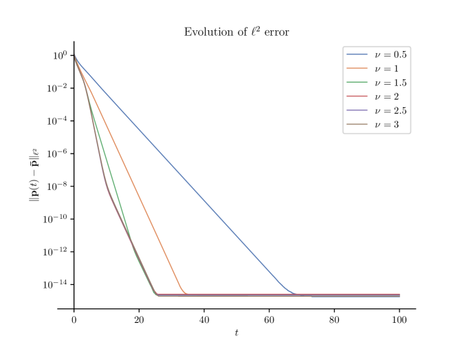
Figure 7: Evolution of the $\ell^{2}$ error $\left\lVert{\bf p}(t)-\mkern 1.5mu\overline{\mkern-1.5mu\bf p\mkern-1.5mu}\mkern 1.5mu\right\rVert_{\ell^{2}}$ over time for different values of $\nu$. It can be seen that larger values of $\nu$ (or $\mu$) leads to faster convergence, although such improvement in terms of the convergence rate saturates when $\nu$ becomes large enough.

To illustrate the quantitative convergence guarantee reported in Theorem 3 we plot the evolution of the $\ell^{2}$ error $\|{\bf p}(t)-\mkern 1.5mu\overline{\mkern-1.5mu\bf p\mkern-1.5mu}\mkern 1.5mu\|_{\ell^{2}}$ over time (see Figure 7) with $\nu\in\{0.5,1,1.5,2,2.5,3\}$, under the same set-up as used for Figure 5. We observe the exponential decay of $\|{\bf p}(t)-\mkern 1.5mu\overline{\mkern-1.5mu\bf p\mkern-1.5mu}\mkern 1.5mu\|_{\ell^{2}}$ as predicted by Theorem 3, although our analytical rate might be sub-optimal for $\nu\geq 1$.

5 Conclusion

In this manuscript, we adopted a kinetic perspective and investigated the continuous-time version of the so-called dispersion process (on a complete graph with $N$ vertices) introduced and studied in a number of recent works [17, 19, 24, 37]. Instead of the probabilistic approach employed in the aforementioned papers, we make use of the classical kinetic theory [39] and focus on the analysis of the associated mean-field system of nonlinear ODEs. We also emphasize that via the identification of particles as dollars and vertices (or sites) as agents, it is possible to reformulate the model using econophysics terminologies as well [20, 15, 28, 35, 36], and such reinterpretation of the dispersion model enables us to design and create intriguing models for econophysics literature.

This work also leaves some important follow-up problems which deserve their own treatments and attentions. For instance, it is possible to prove a (uniform in time) propagation of chaos result in order to make the derivation of the mean-field ODE system (1.6) rigorous? Can one design a natural Lyapunov functional associated to the solution of the nonlinear ODE system (1.6) when $\mu>1$? Lastly, we are also wondering the possibility of sharpening the quantitative $\ell^{2}$ convergence guarantee provided by Theorem 3, as numerical simulations suggest that we might hope for a decay of the form $\mathrm{e}^{-2t}$ when $\nu>2$.

Acknowledgement  It is a great pleasure to express our gratitude to Sebastien Motsch for generating Figure 1 that illustrates the dispersion model under investigation. The second author is partially supported by the NSF grant: DMS 2054888.

References

- [1] John M. Ball, Jack Carr, and Oliver Penrose. The Becker-Döring cluster equations: basic properties and asymptotic behaviour of solutions. Communications in Mathematical Physics, 104:657–692, 1986.
- [2] John M. Ball, and Jack Carr. The discrete coagulation-fragmentation equations: existence, uniqueness, and density conservation. Journal of Statistical Physics, 61:203–234, 1990.
- [3] John M. Ball, and Jack Carr. Asymptotic behaviour of solutions to the Becker-Döring equations for arbitrary initial data. Proceedings of the Royal Society of Edinburgh Section A: Mathematics, 108(1-2):109–116, 1988.
- [4] Bruce M.Boghosian, Merek Johnson, and Jeremy A. Marcq. An Theorem for Boltzmann’s Equation for the Yard-Sale Model of Asset Exchange: The Gini Coefficient as an Functional. Journal of Statistical Physics, 161:1339–1350, 2015.
- [5] Fei Cao, and Stephanie Reed. A biased dollar exchange model involving bank and debt with discontinuous equilibrium. arXiv preprint arXiv:2311.07851, 2023.
- [6] Fei Cao, and Nicholas F. Marshall. From the binomial reshuffling model to Poisson distribution of money. Networks and Heterogeneous Media, 19(1):24–43, 2024.
- [7] Fei Cao, and Sebastien Motsch. Derivation of wealth distributions from biased exchange of money. Kinetic & Related Models, 16(5):764–794, 2023.
- [8] Fei Cao, Pierre-Emannuel Jabin, and Sebastien Motsch. Entropy dissipation and propagation of chaos for the uniform reshuffling model. Mathematical Models and Methods in Applied Sciences, 33(4):829–875, 2023.
- [9] Fei Cao. Explicit decay rate for the Gini index in the repeated averaging model. Mathematical Methods in the Applied Sciences, 46(4):3583–3596, 2023.
- [10] Fei Cao, and Pierre-Emannuel Jabin. From interacting agents to Boltzmann-Gibbs distribution of money. arXiv preprint arXiv:2208.05629, 2022.
- [11] Fei Cao, and Sebastien Motsch. Sticky dispersion on the complete graph: a kinetic approach. arXiv preprint arXiv:2404.08868, 2024.
- [12] Fei Cao, and Sebastien Motsch. Uncovering a two-phase dynamics from a dollar exchange model with bank and debt. SIAM Journal on Applied Mathematics, 83(5):1872–1891, 2023.
- [13] Fei Cao, and Roberto Cortez. Uniform propagation of chaos for a dollar exchange econophysics model. European Journal of Applied Mathematics, 1–13, 2024.
- [14] Anirban Chakraborti, and Bikas K. Chakrabarti. Statistical mechanics of money: how saving propensity affects its distribution. The European Physical Journal B-Condensed Matter and Complex Systems, 17(1):167–170, 2000.
- [15] Anirban Chakraborti, Ioane Muni Toke, Marco Patriarca, and Frédéric Abergel. Econophysics review: I. Empirical facts. Quantitative Finance, 11(7):991–1012, 2011.
- [16] Arnab Chatterjee, Bikas K. Chakrabarti, and Subhrangshu Sekhar Manna. Pareto law in a kinetic model of market with random saving propensity. Physica A: Statistical Mechanics and its Applications, 335(1-2):155–163, 2004.
- [17] Colin Coopery, Andrew McDowellz, Tomasz Radzikx, and Nicolás Rivera. Dispersion processes. Random Structures & Algorithms, 53(4):561–585, 2018.
- [18] Roberto Cortez, and Joaquin Fontbona. Quantitative propagation of chaos for generalized Kac particle systems. The Annals of Applied Probability, 26(2):892–916, 2016.
- [19] Umberto De Ambroggio, Tamás Makai, and Konstantinos Panagiotou. Dispersion on the complete graph. arXiv preprint arXiv:2306.02474, 2023.
- [20] Adrian Dragulescu, and Victor M. Yakovenko. Statistical mechanics of money. The European Physical Journal B-Condensed Matter and Complex Systems, 17(4):723–729, 2000.
- [21] Bertram Düring, Daniel Matthes, and Giuseppe Toscani. Kinetic equations modelling wealth redistribution: a comparison of approaches. Physical Review E, 78(5):056103, 2008.
- [22] Manuel L. Esquivel. Probability generating functions for discrete real-valued random variables. Theory of Probability & Its Applications, 52(1):40–57, 2008.
- [23] Lawrence C. Evans. Partial differential equations. American Mathematical Society, Vol. 19, 2022.
- [24] Alan Frieze, and Wesley Pegden. A note on dispersing particles on a line. Random Structures & Algorithms, 53(4):586–591, 2018.
- [25] Gustaf Gripenberg, Stig-Olof Londén, and Olof Staffans. Volterra integral and functional equations. Cambridge University Press, 1990.
- [26] Els Heinsalu, and Patriarca Marco. Kinetic models of immediate exchange. The European Physical Journal B, 87(8):1–10, 2014.
- [27] Pierre-Emmanuel Jabin, and Barbara Niethammer. On the rate of convergence to equilibrium in the Becker–Döring equations. Journal of Differential Equations, 191(2):518–543, 2003.
- [28] Ryszard Kutner, Marcel Ausloos, Dariusz Grech, Tiziana Di Matteo, Christophe Schinckus, and H. Eugene Stanley. Econophysics and sociophysics: Their milestones & challenges. Physica A: Statistical Mechanics and its Applications, 516:240–253, 2019.
- [29] Johann-Heinrich Lambert. Observationes variae in mathesin puram. Acta Helvetica, 3(1):128-168, 1758.
- [30] Nicolas Lanchier. Rigorous proof of the Boltzmann–Gibbs distribution of money on connected graphs. Journal of Statistical Physics, 167(1):160–172, 2017.
- [31] Nicolas Lanchier, and Stephanie Reed. Rigorous results for the distribution of money on connected graphs (models with debts). Journal of Statistical Physics, 176(5):1115–1137, 2019.
- [32] Daniel Matthes, and Giuseppe Toscani. On steady distributions of kinetic models of conservative economies. Journal of Statistical Physics, 130(6):1087–1117, 2008.
- [33] Barbara Niethammer. On the evolution of large clusters in the Becker-Döring model. Journal of Nonlinear Science, 13:115–122, 2003.
- [34] Barbara Niethammer. A scaling limit of the Becker-Döring equations in the regime of small excess density. Journal of Nonlinear Science, 14:453–468, 2004.
- [35] Eder Johnson de Area Leão Pereira, Marcus Fernandes da Silva, and HB de B. Pereira. Econophysics: Past and present. Physica A: Statistical Mechanics and its Applications, 473:251–261, 2017.
- [36] Gheorghe Savoiu. Econophysics: Background and Applications in Economics, Finance, and Sociophysics. Academic Press, 2013.
- [37] Yilun Shang. Longest distance of a non-uniform dispersion process on the infinite line. Information Processing Letters, 164:106008, 2020.
- [38] Alain-Sol Sznitman. Topics in propagation of chaos. In Ecole d’été de probabilités de Saint-Flour XIX—1989, pages 165–251. Springer, 1991.
- [39] Cédric Villani. A review of mathematical topics in collisional kinetic theory. Handbook of mathematical fluid dynamics, 1:71–305, 2002.