Digital Twins of the EM Environment:
Benchmark for Ray Launching Models

Abstract

Digital Twin has emerged as a promising paradigm for accurately representing the electromagnetic (EM) wireless environments. The resulting virtual representation of the reality facilitates comprehensive insights into the propagation environment, empowering multi-layer decision-making processes at the physical communication level. This paper investigates the digitization of wireless communication propagation, with particular emphasis on the indispensable aspect of ray-based propagation simulation for real-time Digital Twins. A benchmark for ray-based propagation simulations is presented to evaluate computational time, with two urban scenarios characterized by different mesh complexity, single and multiple wireless link configurations, and simulations with/without diffuse scattering. Exhaustive empirical analyses are performed showing and comparing the behavior of different ray-based solutions. By offering standardized simulations and scenarios, this work provides a technical benchmark for practitioners involved in the implementation of real-time Digital Twins and optimization of ray-based propagation models.

I Introduction

The accurate modeling of electromagnetic (EM) radio maps has significant implications for improving key parameters in network design and deployment [1]. Within this context, the concept of the Digital Twin (DT) emerges, representing a sophisticated but interesting approach to constructing precise digital replicas of physical entities or processes. These DTs provide real-time insight into their corresponding physical counterparts, effectively integrating simulations with existing databases [2]. This framework necessitates the development of appropriate models for the continuous update and enhancement of the virtual representations, ensuring their matching with real-world entities. Achieving this correspondence enables a closed-loop system in which decisions concerning the physical entity are informed by real-time data derived from the DT.

In addressing the demands of modeling and designing radio maps tailored to the dynamic and complex environments in the forthcoming sixth-generation (6G) networks, the DT presents a compelling avenue. In fact, by leveraging high-definition three-dimensional (3D) maps, DT-enabled network systems can achieve precise real-time digital representations of the EM environment and radio maps. DT effectiveness can be improved by incorporating multimodal sensory data from different entities in the network, including user equipment, connected vehicles, drones, in conjunction with a comprehensive description of the state of the communication network  [3].

Wireless propagation is notably featured by multipath propagation. Ray-based propagation simulation stands as a versatile modeling tool, offering estimates of path loss, angle of arrival/departure, propagation delay, and Doppler shift for each multipath component. Functionally, ray-based propagation simulation relies on the high-frequency approximation of Maxwell’s equations, which results in the concept of ray. Furthermore, it allows for effective integration with 3D scenarios maps to dynamically and faithfully model the propagation environment with rich geometric features [4].

Different organizations have proposed computational engines to perform ray-based propagation simulations, and by integrating those software into the DT-enabled network systems, it is possible to better simulate the real-world conditions of the EM environment in urban settings, where the propagation of high-frequency signals is significantly affected by the urban landscape. By accounting for different possible interactions with the environment— e.g., reflections, diffractions, and diffuse scattering— we can achieve more accurate estimates and designs for wireless communication systems. Specifically in dynamic scenarios, such as vehicular ones, traditional models may fail to accurately represent channel characteristics [5]. As research on DT-enabled network systems continues, it becomes incrementally more relevant to assess and understand their integration with ray-based propagation simulations.

Ray-based propagation simulations are expensive, and therefore substantial research efforts have been directed towards enhancing computational speed [6, 7, 8, 9, 10]. In [6] a simplification of simulations based on ray-based models is proposed and evaluated in end-to-end networks. An alternative dynamic ray-based method that is in [7] alleviates the computational load of ray-based models. An adaptive ray launching algorithm is proposed for urban environments [8], reducing its computational burden. The high-fidelity 3D model of the city of Boston, introduced in [9], offers easier integration into DT-enabled systems. In [10] a simplification of building representation is proposed for ray models.

The computational burden associated with ray-based propagation simulations can easily become the bottleneck towards achieving real-time performance in the update of a DT. In addition, the dynamism of the environment may render the simulation outdated even before the end of its computation.

Contributions. In this paper, we aim to provide a technical benchmark to evaluate the computational performance of different ray-based simulation software. The main contributions are summarized below:

• Definition of an empirical benchmark to evaluate and compare the computational performance of ray-based simulation software in two different urban scenarios characterized by their geometrical representation complexity.

• Evaluation of time performance for a selection of ray-based simulation software in the proposed urban scenarios and wireless link configurations— i.e., single link vs. simultaneous multiple links; the latter is evaluated with GPU acceleration (when applicable). The evaluation has been carried out for increasing ray interaction depth, with/without diffuse scattering, and variation in ray launching parameter.

• The 3D meshes of the evaluation scenarios and the source code to replicate the benchmark for the evaluated solutions are available. Fostering a repeatable benchmark with standardized approach to evaluate the computational performance of diverse ray-based propagation algorithms, spanning different implementations and hardware architectures.

By establishing shared simulation settings and scenarios, researchers and developers gain a comprehensive framework for in-depth comparison and analysis of the efficiency of their methodologies. The definition of a standardized methodology promotes transparency and repeatability in research, driving advances in ray-based propagation modeling, and addressing the evolving needs wireless communication systems.

Organization. The remainder of this article is structured as follows: in Sec. II, we provide an overview of the basic ray-based simulation algorithms. Section III describes the 3D maps of the urban environments considered in our simulations, the type of wireless link configurations, and the proposed benchmark framework. Sec. IV provides a brief review of software that implements ray-based models. In Sec. V, we report the simulation results on the comparison of the selected ray-based simulation software. Section VI provides an overview and some remarks about the compared solutions, while in Sec. VII, we draw the conclusions.

II Ray-based propagation algorithms

Following the distinction done in  [11], ray-based models can be differentiated into exact ray computation (ray tracing) and approximated (ray launching):

• Ray Launching (RL), which is an approximate algorithm based on spawning rays from an EM emission source towards a set of angular discretized directions. For each launched ray, after a number of interaction steps (usually a simulation parameter) with the propagation environment, the reception of the ray at a target receiver is checked—e.g., by means of ray-tube modeling [12] or testing if the ray hits a sphere of given (possibly parametric) radius centered at the receiver position. The goal of plain ray launching is not exact point-to-point propagation modeling. Instead, ray launching is particularly suitable for large-scale approximate propagation simulation. One realization of ray launching is the shooting and bouncing rays method discussed below.

• Ray Tracing (RT), which aims at modeling point-to-point propagation by determining the geometrically exact propagation paths between an EM emission source and a target receiver location. According to Reif et al. in [13], ”the exact solution of a 3D optical system consisting of linear reflective surfaces and partially reflective surfaces is undecidable”. The computational time of the ray tracing task can easily become intractable with the increase of the number of surfaces to be taken into account or with the maximum number of interaction points per ray to be considered. The image method, discussed below, is a realization of the ray tracing method for reflection interaction types.

Ray launching and ray tracing lead to a set of fundamental algorithms in high-frequency computational EM, among which are the main ones discussed in the following.

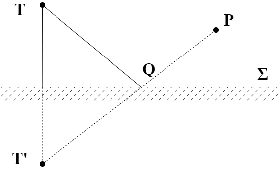
(a) Image method

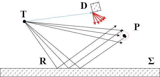
(b) Shooting and Bouncing Rays

Figure 1: LABEL:sub@fig:_Image_method Image Method; T^′ is the image of transmitter T with respect to the reflection plane $\Sigma$. LABEL:sub@fig:_SBR Shooting and Bouncing Rays method; R indicates reflection points, D a diffraction point at an edge, and a path is considered at the receiver if it satisfies the reception condition—exemplified by hitting a reception sphere (red circle) at receiver P.

Image Method [RT]: The image method is a point-to-point propagation simulation method. As such, it is a realization of the above-discussed ray tracing method. We provide in Fig. 1a a graphical representation of the image method for the single reflection case. Referring to Fig. 1a, the trajectory of the ray reflected from a plane surface can be determined as follows: T^′ is computed as the image of transmitter T with respect to the reflection plane $\Sigma$; then T^′ and P are connected through a segment that intersects the plane at point Q; the reflected ray is determined by the segments connecting (T, Q, P). In case of multiple reflections, the method can be extended recursively taking into consideration different reflection planes. The image method becomes computationally taxing when the environment presents an abundant number of reflecting surfaces or the number of sequential interactions considered for a ray increases [4].

Shooting and Bouncing Rays (SBR) [RL]: is a realization of the ray launching approach. A graphical representation is provided in Fig. 1b. A set of rays is launched from the transmitter T with a given angular separation. In conventional implementations, the launched rays are propagated in the environment up to a maximum number of interactions with surfaces, and are considered to reach the receiver P if they meet a reception condition— e.g., intersecting a sphere centered at the receiver P with radius proportional to the distance traveled by the ray. SBR implementations can consider a variety of environmental interactions, e.g., reflection, diffraction, and diffuse scattering. The latter has been shown to be particularly relevant to accurately model urban propagation environments[14].

Path correction methods [RL and RT]: In SBR, the exact reception of a ray at a given target point in space is highly unlikely owing to the discrete angular resolution of ray launching. For this reason, path correction methods [4] have been proposed to exploit both the computational efficiency of SBR and the exact geometric accuracy of the image method. This is achieved by slightly changing the positions of the intermediate path interaction points on the surfaces so that the launched ray can exactly hit the target point. Examples of path correction methods are implemented in the SBR models proposed by [15] and [16].

Differentiable Ray Tracing [RL or RT]: A new approach to ray modeling based on differentiable rendering (DR) [17] has recently been proposed in [18]. The developed procedure is based on Mitsuba 3 [19] DR system— which, in turn, leverages the Dr.Jit just-in-time (JIT) compiler [20]. DR for ray simulation brings as a key advantage differentiability with respect to environmental (e.g., objects’ radio-materials parameters) and system (e.g., antenna arrays positions) of the ray tracing procedure. In [18], both an exhaustive ray tracing method and an approximate SBR-based approach are proposed. The exhaustive method tests all the possible combinations of mesh triangles and edges— leading to high accuracy but intractable computational time. The ray launching method provides a trade-off between accuracy and complexity by means of a sampling scheme on the ray launching sphere. In [21], the authors tackle the challenges of integrating ray tracing into DR systems, proposing a new fully differentiable framework with continuous loss function through local smoothing.

III Benchmark framework

(a) Scenario1

(b) Scenario2

Figure 2: Details of the 3D meshes of the two proposed scenarios. The view in LABEL:sub@fig:_Wireframe_Scenario1 highlights the level of detail in Carla w.r.t. LABEL:sub@fig:_Wireframe_Scenario2, which is the view of the OSM scenario characterized by a lower level of details. In LABEL:sub@fig:_Wireframe_Scenario2, the main building of the High Frequency campus, Italy is in green.

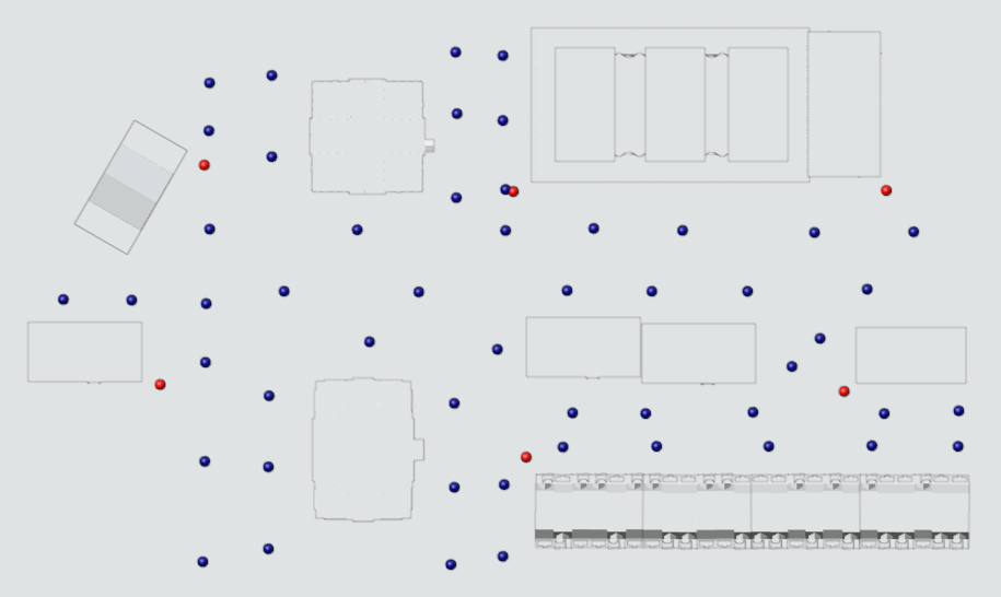
(a) Scenario1

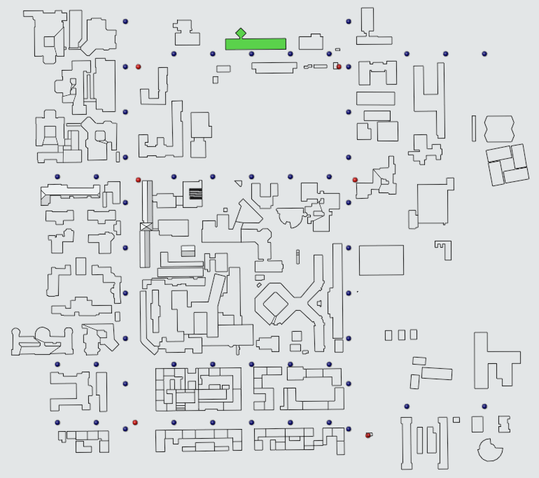
(b) Scenario2

Figure 3: Top views of the selected evaluation scenarios along with the chosen Tx (red spheres) and Rx (blue spheres) positions. In (b), the main building of the High Frequency Campus in Milan, Italy is in green.

In what follows, we describe urban scenarios, wireless link configurations, and the proposed benchmark framework to evaluate the ray-based method considered.

III-A Evaluation scenarios

We have selected two urban evaluation scenarios, differentiated by the level of complexity of the buildings’ meshes by which they are composed. Figure 2 shows the mesh complexity of the proposed scenarios.

• CARLA High Definition Mesh (Scenario1): It is an environment composed by complex realistic 3D buildings’ meshes retrieved from the Town 10 urban scenario available within the realistic CARLA automotive simulator [22]. Town 10 represents a typical inner-city environment, composed of, e.g., skyscrapers, hotels, public buildings, and apartment blocks. We have considered a selection of buildings in Town 10 that led to a diversified urban environment, and we exported the corresponding 3D meshes using the CARLA Unreal Engine editing interface. The resulting 3D mesh is represented in Fig. 2a.

• OSM Low Definition Mesh (Scenario2): As the second test environment, we consider a scenario composed by simplified 2.5D buildings’ meshes—i.e., meshes defined by their outline on the ground and their height—retrieved from the OpenStreetMap (OSM) [23] online service for the High Frequency Campus urban geographical area in Milan, Italy. A section of the scenario is reported in Fig. 2b, showing the simplicity of the building representation in this setting.

III-B Wireless link configurations

Let $\mathcal{G}$ be a generic set of transceiver configurations, $\mathcal{T}$ be the set of transmitters, $\mathcal{R}$ be the set of receivers. A generic transceiver configuration is defined as $g_{k}\coloneq a_{k}\cup b_{k}$ where $a_{k}\subseteq\mathcal{T}$ and $b_{k}\subseteq\mathcal{R}$. Denoting $N_{Tx}=|\mathcal{T}|$, $N_{Rx}=|\mathcal{R}|$ the number of transmitters and receivers.

We define two distinct link configurations, represented by $\mathcal{G}_{1}$ and $\mathcal{G}_{2}$:

• Single Link (SL) configurations: the set $\mathcal{G}_{1}$ represents the set of all Tx/Rx pairs. Ray computations and wall-clock time measurement are performed for $g_{ij}$ with $i=1,2,...,N_{Tx}$ and $j=1,2,...,N_{Rx}$. This approach captures the performance of the ray model without parallelization.

• Multi Link (ML) configurations: a transceiver configuration $g_{i}\in\mathcal{G}_{2}$ is defined as $g_{i}=T_{i}\cup\mathcal{R}$ with $i=1,2,...,N_{Tx}$. Measurements and computations are performed for the configurations in $\mathcal{G}_{2}$ simulating a channel propagation scenario with one transmitter and multiple receivers. This allows the different ray methods to exploit hardware parallelization and algorithmic optimization in realistic use cases.

Generic link configurations can be defined and characterized by their set of transceiver configurations $\mathcal{G}$, each different configuration can be designed to suit different use cases and capture different properties of the ray methods. The algorithm in 1 is the pseudo code for a generic simulation with set $\mathcal{G}$, measurements of the wall-clock time are performed after the transceivers in $g_{k}\in\mathcal{G}$ are loaded into memory. If round-trip-time measurements are more desirable, include the loading of the configuration $g_{k}$ within the simulation software.

The $N_{Tx}=6$ transmitters are placed in nodal positions in urban environments at a height of 7 m, while the $N_{Rx}=51$ receivers are distributed along roads at a height of 1.5 m. Each transmitter (Tx) and each receiver (Rx) are equipped with the same type of isotropic antennas. In Fig. 3 the positions of the transmitters (red spheres) and receivers (blue spheres) are shown. When required, the simulation boundary was set with a 50 m margin with respect to the bounding box comprising all buildings. The simulation boundary is assumed to be absorbing, so that only rays interacting with the buildings and ground within the scenario are considered. The ITU recommendation [24] has been considered as reference to determine the required EM properties (relative permittivity and conductivity) of the radio materials. The simulation parameters that are common for each scenario are summarized in Table I.

1:$\mathcal{T}\coloneq$ set of transmitters, $\mathcal{R}\coloneq$ set of receivers.
$\mathcal{G}\coloneq$ set of transceiver configurations, $g_{k}=a_{k}\cup b_{k}$ with $g_{k}\in\mathcal{G}$, $a_{k}\subseteq\mathcal{T}$, and $b_{k}\subseteq\mathcal{R}$.

2:$\boldsymbol{t}$ vector of wall-clock time measurements.

3:Initialize $\boldsymbol{t}\in\mathbb{R}^{|\mathcal{G}|}$

4:for all $g_{k}\in\mathcal{G}$ do

5:     load_transmitters($a_{k}$)

6:     load_receivers($b_{k}$)

7:     $t^{\prime}=$ current_timestamp()

8:     compute_paths($g_{k}$)

9:     $t_{k}=$ current_timestamp() $-\ t^{\prime}$

10:end for

11:return $\boldsymbol{t}$

Algorithm 1 Simulation pseudocode.

TABLE I: Simulation parameters.

Parameter	Value
Antenna Type	Isotropic
Carrier frequency	28 GHz
Buildings and ground material	Concrete
Material relative permittivity	5.31
Material conductivity	0.4838 S/m
Tx height, Rx height	7 m , 1.5m
$N_{Tx}$, $N_{Rx}$	6, 51

III-C Benchmark workflow

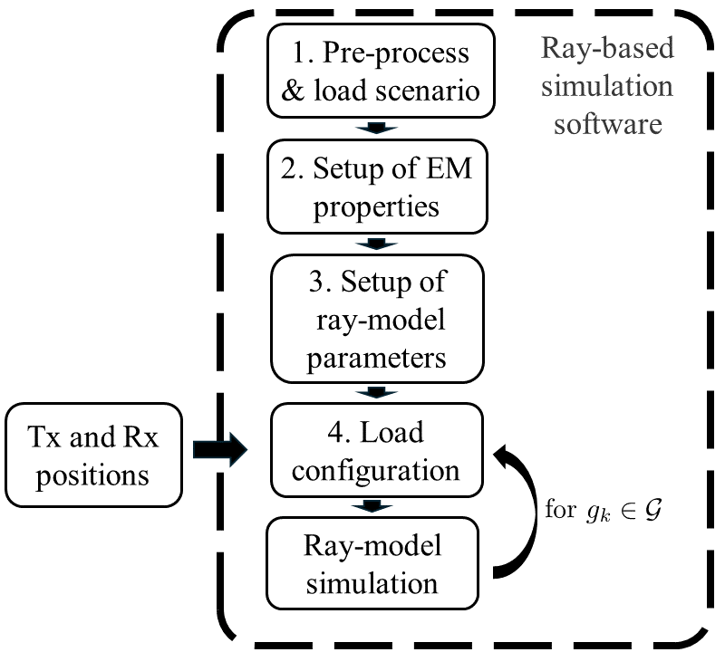
Figure 4: Benchmark workflow. $\mathcal{G}$ is a set of transceiver configurations and $g_{k}$ is a specific configuration containing transmitters and receivers.

Given a ray-based simulation software, a scenario, and a configuration $\mathcal{G}$. The benchmark workflow can be described as follows.

1. Pre-process & load scenario. Ray-based model simulation requires 3D meshes of the environment as input. These meshes may not be in a format compatible with the specific ray-based simulation software. If necessary, the scenario is converted from its original format into a supported one before loading it within the simulation software. This ensures that the simulation software can accurately interpret and utilize the environmental data.

2. Setup of EM properties. In this step, the EM properties of the scenario are configured. This includes defining parameters such as permittivity, permeability, and conductivity of materials within the simulation environment, according to the specifications in Table I.

3. Setup of ray model parameters. Different software implementations of ray models may offer various configurable parameters. This step involves aligning and configuring these parameters to ensure consistency across different simulations.

4. Load configuration. Transmitters and receivers in the configuration are loaded within the simulated scenario at positions provided from an external file.

5. Ray-model simulation. This step is the core computational step where the actual simulation of the ray model is performed. The software computes the paths that rays take as they propagate from the transmitters to the receivers. The wall-clock time is measured in this step.

Steps 4. and 5. are repeated until the configurations $g_{k}\in\mathcal{G}$ are exhausted. Figure 4 summarizes the benchmark workflow.

IV Comparison of ray-based simulation software

In this section, we review the examined ray-based simulation software. Open-source and commercial software embeds ray-based models for EM propagation modeling. Among the most widely used commercial software are Remcom Wireless InSite [15], MathWorks RF Antenna Toolbox [16], Siradel Volcano [25], Altair Feko [26], iBware Design and iBware Reach [27], and EDX SignalPro [28]. NVIDIA Sionna [29] and Ns-3 mmWave Module [30] instead provide open source solutions. Based on the availability of proprietary software, we evaluate the following ray-based simulation software.

Remcom Wireless InSite (v3.3.3) [15] is a commercial software that provides several methods for the analysis of radio propagation and wireless communication systems in various conditions (i.e., indoor, outdoor, and rural areas). Widely used for wireless propagation simulation in the relevant literature [31, 32], it provides an efficient and accurate modeling of the characteristics of the communication channel in complex EM propagation environments. It offers two ray optical computation models allowing generic 3D environments: (i) full 3D, supporting simulations in the 0.1-20 GHz frequency range by means of SBR and Eigen Ray algorithms, and (ii) X3D, which supports simulations in the 0.1-100 GHz frequency range and integrates SBR with a path correction algorithm adjusting the interaction points to obtain exact propagation paths between Tx and Rx. Moreover, X3D supports diffuse scattering simulation, which has been shown to be particularly relevant for accurately modeling urban propagation environments [14].

NVIDIA Sionna RT (v0.16.2) [18] is a recently proposed differentiable ray optical engine that is part of the NVIDIA Sionna link-level simulation library [29]. NVIDIA Sionna RT allows for accurate ray simulations taking account of reflection, diffraction, and diffuse scattering interactions of propagation paths with the environment. As reported in Sec. II, it implements differentiable rendering providing a flexible framework that allows to include the communication channel within end-to-end optimization procedures. Sionna RT provides two ray-based methods: (i) an exhaustive method, which tests all possible combinations of 3D primitives and paths and becomes computationally intractable for high path depths—i.e., number of interaction points per path—or number of surfaces in the scene, and (ii) a Fibonacci method, which uses the SBR approach to efficiently compute the propagation paths and implements a sampling procedure for ray launching that enables a trade-off between simulation accuracy and computational time.

MathWorks Ray tracing model (vR2023a U1) [16] is part of the MathWorks Antenna Toolbox and offers two ray optical computation methods: (i) SBR implementation with exact path correction, supporting up to 10 reflection and 2 edge diffractions and providing an approximate number of propagation rays; (ii) a ray tracing model based on the image method, supporting a maximum of 2 path reflections and providing an exact number of rays featured by line-of-sight or reflection with exact geometry. Both methods enable simulation in the 0.1-100 GHz frequency range and support generic 3D indoor and outdoor environments.

V Numerical results

In this section, we evaluate the computational time efficiency of the considered ray-based methods in Scenario1 and Scenario2. Also we produce the radio map from the different simulation software. Our simulations are performed on a Windows 10 workstation equipped with Intel(R) Core(TM) i7-9700K CPU@3.60 GHZ, 8 cores, 16 GB RAM, and NVIDIA GeForce GTX 1070 Ti GPU with 8GB of dedicated memory.

V-A Computational Time

(a) SL Scenario2: WI X3D

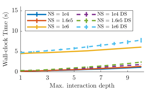
(b) SL Scenario2: Sionna Fibonacci CPU

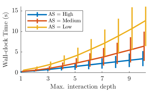
(c) SL Scenario2: MW SBR

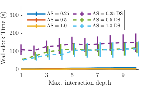
(d) ML Scenario2: WI X3D

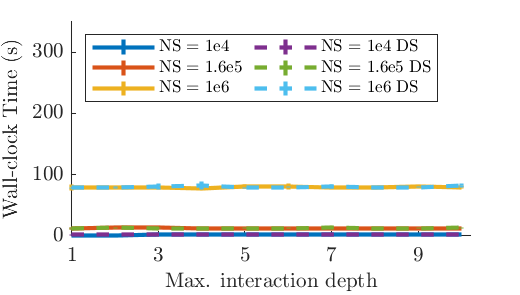
(e) ML Scenario2: Sionna Fibonacci GPU

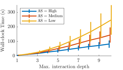
(f) ML Scenario2: MW SBR

Figure 5: Single Link (SL) and Multi Link (ML) configurations in Scenario2 with 1$\sigma$ errorbar with respect to the maximum interaction depth, varying angular separation (AS) or number of samples (NS), with (solid line) or without (dashed line) Diffuse Scattering (DS).

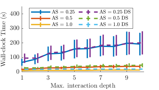
(a) SL Scenario1: WI X3D

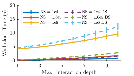
(b) SL Scenario1: Sionna Fibonacci CPU

Figure 6: Single Link configurations in Scenario1 with 1$\sigma$ errorbar with respect to the maximum interaction depth, varying angular separation (AS) or number of samples (NS), with (solid line) or without (dashed line) Diffuse Scattering (DS).

(a) Scenario1: WI X3D

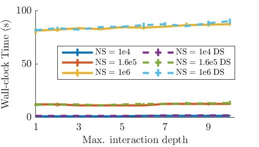
(b) Scenario1: Sionna Fibonacci GPU

Figure 7: Multiple Link configurations in Scenario1 with 1$\sigma$ errorbar with respect to the maximum interaction depth, varying angular separation (AS) or number of samples (NS), with (solid line) or without (dashed line) Diffuse Scattering (DS).

As discussed in Sec. III we consider a set of transmitters $\mathcal{T}$, a set of receivers $\mathcal{R}$. The wall-clock time $t_{k}$ is measured during the ray computation, for each transceiver configuration $g_{k}\in\mathcal{G}$. Sample mean $\mu$ and variance $\sigma^{2}$ are evaluated for the specific Single Link (SL) and Multi Link (ML) simulation, with $K=|\mathcal{G}|$ as:

$$\mu =\frac{1}{K}\sum_{k=1}^{K}t_{k},$$ (1)

$$\sigma^{2} =\frac{1}{K-1}\sum_{k=1}^{K}(t_{k}-\mu)^{2}.$$

(a) Single Link configurations on Scenario1

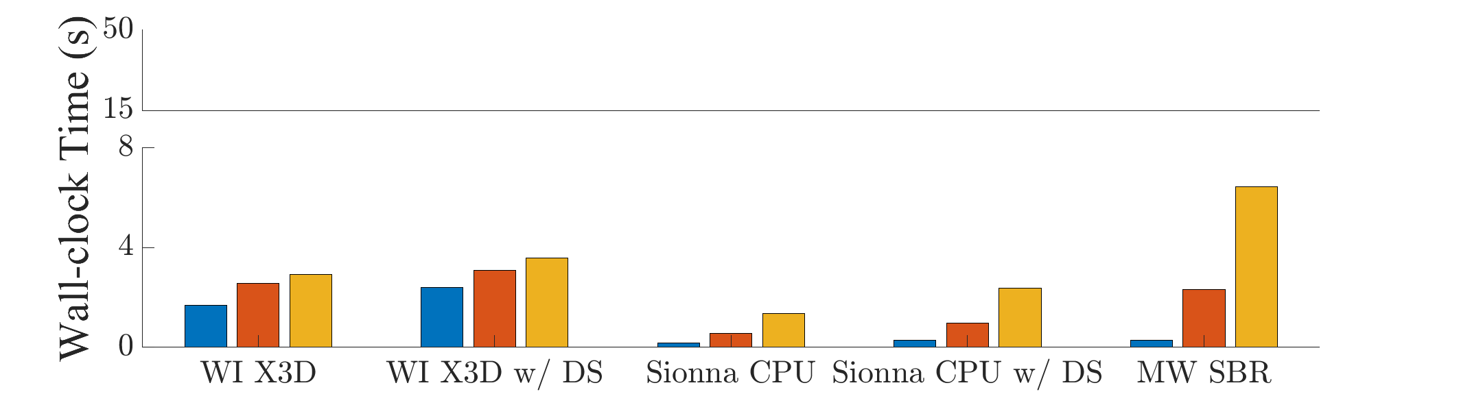
(b) Single Link configurations on Scenario2

(c) Multiple Link configurations on Scenario1

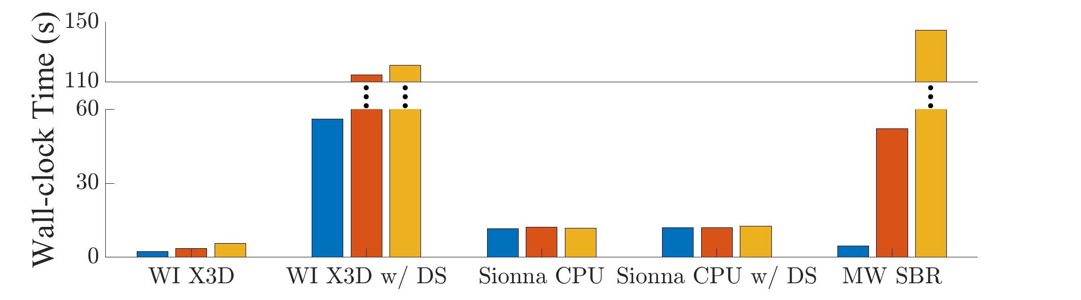
(d) Multiple Link configurations on Scenario2

Figure 8: Comparison of the selected ray-based simulation software over a comparable initial number of rays at Tx. WI X3D AS $=0.5$ deg, MW SBR AS = Medium, Sionna Fibonacci NS $=1.6e5$.

TABLE II: Software-specific ray launching simulation parameters.

Software	Parameter	Value
Remcom Wireless InSite (v3.3.3)	RT method	X3D
	Angular separation	[0.25, 0.5, 1.0] deg
	Diffractions num.	1
	Diffuse scattering	$(R=2,D=1)$
MathWorks Ray Tracing Model (vR2023a U1)	RT method	SBR
	Angular separation	[low, medium, high]
	Diffractions num.	1
NVIDIA Sionna RT (v0.16.2)	RT method	Fibonacci
	Num. of samples	[1e4, 1.6e5, 1e6]
	Diffractions num.	True
	Diffuse scattering	True

We consider the X3D model for Remcom Wireless InSite (WI X3D), the SBR with exact path correction model for the MathWorks ray launching model (MW SBR), and the Fibonacci model for NVIDIA Sionna RT. MW SBR has been performed within its Graphical User Interface (GUI), adding a negligible overhead in terms of computational time, and the software cannot handle Scenario1 on our workstation.

Ray launching algorithms are significantly impacted by the initial number of rays sampled at the Tx. Both WI X3D and MW SBR offer the flexibility to specify the angular separation (AS) in degrees between the launched rays, while Sionna Fibonacci allows for the specification of the number of samples (NS)— e.g., the number of candidate rays split equally among the Tx during the simulation. Simulations are performed for the two proposed scenarios, SL/ML configurations, and increasing maximum interaction depth. For Sionna Fibonacci, this parameter encompasses any type of ray interaction, whereas for WI X3D and MW SBR, it specifically pertains to the maximum number of reflections. The varying parameters for each ray launching methods are summarized in Table II, while the unmentioned parameters are set to default values.

CPUs and GPUs are different types of hardware resources. The former are optimized to handle sequential tasks and general-purpose computing. The latter are particularly useful for handling tasks that require parallel execution and high throughput— Sionna framework allows for finer control of the type of resource used in the computation, in SL configurations we do not enable GPU acceleration, while for ML configurations we enable it.

In Fig. 5, the results of the SL and ML configurations are reported for Scenario2. For SL configurations, it can be observed that for WI X3D and Sionna CPU the addition of diffuse scattering interaction adds a negligible overhead in the computation. MW SBR does not model diffuse scattering. For ML configurations, the WI X3D model observes a significant increase in computational time.

In Fig. 6, the results of the SL configurations for Scenario1 are reported. Scenario1 is characterized by a higher number of meshes— i.e. number of vertices, edges, and faces that defines the shape of the objects in the 3D map. This complexity significantly impairs the ray computations. An inspection between Fig. 5a and 6a highlights the impact of mesh complexity, specifically the addition of diffuse scattering.

In Fig. 7, presents the results of ML configurations for Scenario 1. Figure 7a reports of the computation for WI X3D without diffuse scattering. When diffuse scattering is considered the overall average wall-clock time: is 440 s with maximum interaction depth set to 1 and AS 1.0 deg, while 730 s with maximum interaction depth set to 10 and AS 0.25 deg.

The initial number of rays significantly impacts the computational performance of the ray launching approach. In order to provide a direct comparison, a set of equivalent values is used. The WI X3D AS is set at 0.5 degrees, the MW SBR AS is set as Medium, Sionna Fibonacci NS is set to $1.6e5$. This creates an equivalent starting condition. Figure 8 illustrate the results, showing in each graph a different scenario and a wireless link simulation.

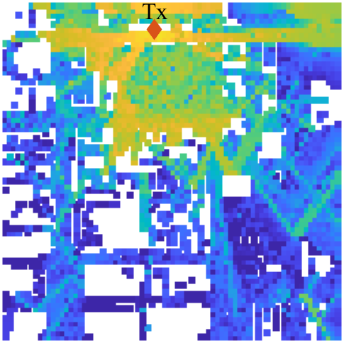
(a) WI X3D

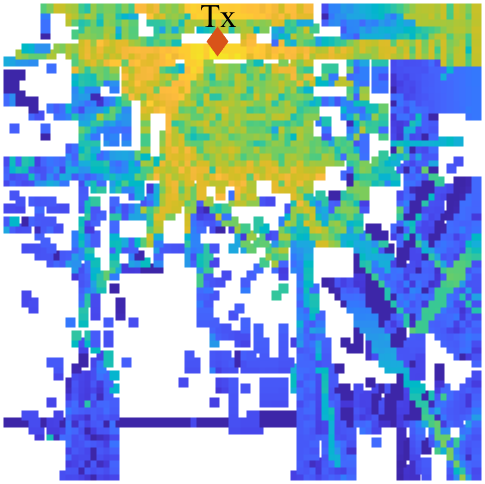
(b) Sionna Fibonacci

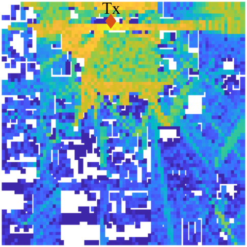
(c) MW SBR

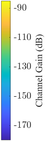
(d)

Figure 9: Channel Gain (dB) of the radio map produced using the evaluated ray-based simulation software. Simulations are performed for a) WI X3D AS = 0.5 deg, b) Sionna Fibonacci NS = 1.6e5, c) MW SBR AS = Medium. WI and MW with maximum 3 reflections and 1 diffraction. Sionna maximum path depth 4. The Tx position is highlighted by a red diamond.

Comparison of Sionna in Fig. 8a and Fig. 8c reveals distinct behaviors in Sionna’s computational time when utilizing CPU versus GPU across increasing interaction depth. The CPU behavior exhibits a linear trend with increasing path depth, whereas the GPU is not affected by path depth. In Fig. 8c Sionna GPU for maximum interaction depth of 1 observes a slightly higher computational time than the counterpart at depth of 5. This is due to the GPU warm-up time and just-in-time compilation overheads. The differentiable ray tracing implementation from Sionna supports the addition of diffuse scattering interactions with the environment without significantly increasing the average wall-clock time.

V-B Radio Map predictions

The three different simulation software are used to calculate the Channel Gain in Scenario2, obtaining the radio maps reported in Fig. 9. These simulations were conducted with the following parameters: for WI X3D, an angular separation (AS) of 0.5 degrees; for MW SBR AS = Medium; and for Sionna, a Fibonacci number of samples (NS) of 1.6e5. WI and MW were configured with a maximum of three reflections and one diffraction, while Sionna was set to a maximum path depth of four.

A single transmitter (Tx) was considered and is located on the top of the main building of the High Frequency Campus in Milan, Italy at height of 21.7 m from the ground. The receivers are uniformly distributed throughout the map area at height of 1.5 m, forming a grid with a resolution of 10 × 10 meters. The carrier frequency is set to 28 GHz, and the Tx and Rxs antennas are isotropic.

Overall, the results are consistent across the three simulators, with differences of only a few dB at specific points. WI X3D and MW SBR offer more detailed insights into the EM radio map, particularly where the Rxs are located far from the Tx. The impact of buildings and obstacles is represented more consistently by these two simulators compared to the Sionna Fibonacci.

The WI X3D, shown in Fig. 9a, integrates the SBR method with a path correction algorithm that adjusts the interaction points to achieve precise propagation paths between the Tx and each Rx. This enhancement is particularly evident in non-line-of-sight points.

Sionna Fibonacci, illustrated in Fig. 9b, lacks channel characterization for certain RX points on the map. This limitation may be due to the underlying Mitsuba differentiable rendering system that is unable to compute the propagation path and/or due to the absence of path correction methods for Sionna Fibonacci.

Simulation	Software	Single Link	Multiple Link	Path Depth Behaviour	DS Behavior
		Performance	Performance	Single/Multiple Link	Single/Multiple Link
Scenario1	Sionna Fibonacci	✓✓	✓✓	linear, constant	$\times$(1.5 to 2), constant
	WI X3D	✓	✓	linear, linear	$\times$(1 to 1.5), $\times$(10 to 25)
Scenario2	Sionna Fibonacci	✓✓✓	✓✓	linear, constant	$\times$(1.5 to 2), constant
	WI X3D	✓✓	✓✓✓	linear, linear	$\times$(1 to 1.5), $\times$(20 to 30)
	MW SBR	✓	✓	linear, linear	N/A

TABLE III: Summary of results over a comparable initial number of rays at Tx. WI X3D AS $=0.5$ deg, MW SBR AS = Medium, Sionna Fibonacci NS $=1.6e5$. Single Link and Multi Link simulation performance, their approximate behavior at increasing maximum interaction depth, and the increase range with respect to the same simulation condition with the diffuse scattering interaction. Each extra tick indicates a better relative wall-clock time in the simulations without diffuse scattering.

In Fig. 9c, the radio map predicted by the MW SBR is shown. The MW software also utilizes an SBR implementation with exact path correction, resulting in a comprehensive characterization of the EM environment.

VI Overview and Discussion

This section aims to summarize the main observations and notable points derived from our simulations. Table III provides an overview of the results evaluated with an equivalent initial number of rays. Each extra tick in the SL and ML performance column indicates a better relative wall-clock time for the given wireless link simulation without diffuse scattering. With an increase in the maximum interaction depth, the behavior is approximately linear for most of the simulations. The diffuse scattering behavior indicates the approximate increase range with respect to the same simulation parameter without the diffuse scattering interaction. Sionna and WI implement different models for the diffuse scattering interaction, as can be observed by their distinct behavior.

The computational performance for ray-based models is a multifaceted task. This includes the meshes of the propagation environment, the underlying computing infrastructure, and any type of algorithmic optimization. The type and number of interactions also significantly affect the simulation times. Conducting a comprehensive analysis from a computational theory standpoint of all these factors is challenging and becomes unfeasible when the source code is unavailable. Instead, benchmarks serve as a practical alternative for evaluating algorithmic implementations and hardware configurations in a black-box manner.

The simulations that compare the radio map using three different software in similar simulations setting showcase consistent results across them with minor discrepancies. WI X3D and MW SBR provided detailed insights into the EM radio map, particularly for distant receiver points, while Sionna Fibonacci lacks characterization for certain RX locations in non-line-of-sight condition.

VII Conclusions

This paper proposes a benchmark of different ray launching solutions, considering several simulation parameters such as the angular separation/number of samples and ray interactions with the environments. Two different urban environments are considered, one with complex mesh detail and one with simpler mesh detail. Two sets of transceiver configurations that evaluate different use cases are tested. The proposed framework allows the practitioner to make an informed decision when selecting the appropriate solution for their application. The availability and reproducibility of the benchmark have the additional advantage of providing a reference point to track advances, ensuring that improvements in computational performance can be systematically monitored and evaluated.

References

- [1] P. Ferrand, M. Amara, S. Valentin, and M. Guillaud, “Trends and Challenges in Wireless Channel Modeling for Evolving Radio Access,” IEEE Communications Magazine, vol. 54, no. 7, pp. 93–99, 2016.
- [2] L. U. Khan, W. Saad, D. Niyato, Z. Han, and C. S. Hong, “Digital-Twin-Enabled 6G: Vision, Architectural Trends, and Future Directions,” IEEE Communications Magazine, vol. 60, no. 1, pp. 74–80, 2022.
- [3] A. Alkhateeb, S. Jiang, and G. Charan, “Real-Time Digital Twins: Vision and Research Directions for 6G and Beyond,” IEEE Communications Magazine, vol. 61, no. 11, pp. 128–134, 2023.
- [4] Z. Yun and M. F. Iskander, “Ray Tracing for Radio Propagation Modeling: Principles and Applications,” IEEE Access, vol. 3, pp. 1089–1100, 2015.
- [5] C. Ding and I. W.-H. Ho, “Digital-Twin-Enabled City-Model-Aware Deep Learning for Dynamic Channel Estimation in Urban Vehicular Environments,” IEEE Transactions on Green Communications and Networking, vol. 6, no. 3, pp. 1604–1612, 2022.
- [6] M. Lecci, P. Testolina, M. Polese, M. Giordani, and M. Zorzi, “Accuracy Versus Complexity for mmWave Ray-Tracing: A Full Stack Perspective,” IEEE Transactions on Wireless Communications, vol. 20, no. 12, pp. 7826–7841, 2021.
- [7] D. Bilibashi, E. M. Vitucci, and V. Degli-Esposti, “On Dynamic Ray Tracing and Anticipative Channel Prediction for Dynamic Environments,” IEEE Transactions on Antennas and Propagation, vol. 71, no. 6, pp. 5335–5348, 2023.
- [8] J. S. Lu, E. M. Vitucci, V. Degli-Esposti, F. Fuschini, M. Barbiroli, J. A. Blaha, and H. L. Bertoni, “A Discrete Environment-Driven GPU-Based Ray Launching Algorithm,” IEEE Transactions on Antennas and Propagation, vol. 67, no. 2, pp. 1180–1192, 2019.
- [9] P. Testolina, M. Polese, P. Johari, and T. Melodia, “BostonTwin: the Boston Digital Twin for Ray-Tracing in 6G Networks,” in ACM Multimedia Systems Conference 2024 (MMSys ’24), 2024.
- [10] Z. Yun and M. F. Iskander, “Simplifying Building Structures for Efficient Radio Propagation Modeling,” in 2023 IEEE International Symposium on Antennas and Propagation and USNC-URSI Radio Science Meeting (USNC-URSI), 2023, pp. 449–450.
- [11] B. Gschwendtner, G. Wölfle, B. Burk, and F. Landstorfer, “Ray Tracing vs. Ray Launching in 3-D Microcell modelling,” in 1st European personal and mobile communications conference (EPMCC), 1995, pp. 74–79.
- [12] M. F. Iskander and Z. Yun, “Propagation Prediction Models for Wireless Communication Systems,” IEEE Transactions on microwave theory and techniques, vol. 50, no. 3, pp. 662–673, 2002.
- [13] J. H. Reif, J. D. Tygar, and A. Yoshida, “Computability and complexity of ray tracing,” Discrete Comput. Geom., vol. 11, no. 3, p. 265–288, dec 1994. [Online]. Available: https://doi.org/10.1007/BF02574009
- [14] V. Degli-Esposti, “A Diffuse Scattering Model for Urban Propagation Prediction,” IEEE Transactions on Antennas and Propagation, vol. 49, no. 7, pp. 1111–1113, 2001.
- [15] Remcom Wireless InSite. [Online]. Available: https://www.remcom.com/wireless-insite-em-propagation-software
- [16] MathWorks radio propagation models. [Online]. Available: https://uk.mathworks.com/help/antenna/ref/rfprop.raytracing.html
- [17] H. Kato, D. Beker, M. Morariu, T. Ando, T. Matsuoka, W. Kehl, and A. Gaidon, “Differentiable rendering: A survey,” arXiv preprint arXiv:2006.12057, 2020.
- [18] J. Hoydis, F. A. Aoudia, S. Cammerer, M. Nimier-David, N. Binder, G. Marcus, and A. Keller, “Sionna RT: Differentiable ray tracing for radio propagation modeling,” arXiv preprint arXiv:2303.11103, 2023.
- [19] “Mitsuba 3 Differentiable Rendering System,” https://www.mitsuba-renderer.org/, accessed on 20 March 2024.
- [20] W. Jakob, S. Speierer, N. Roussel, and D. Vicini, “Dr.Jit: A Just-In-Time Compiler for Differentiable Rendering,” Transactions on Graphics (Proceedings of SIGGRAPH), vol. 41, no. 4, Jul. 2022.
- [21] J. Eertmans, L. Jacques, and C. Oestges, “Fully Differentiable Ray Tracing via Discontinuity Smoothing for Radio Network Optimization,” arXiv preprint arXiv:2401.11882, 2024.
- [22] A. Dosovitskiy, G. Ros, F. Codevilla, A. Lopez, and V. Koltun, “CARLA: An open urban driving simulator,” in Proceedings of the 1st Annual Conference on Robot Learning, 2017, pp. 1–16.
- [23] OpenStreetMap. [Online]. Available: https://www.openstreetmap.org/
- [24] International Telecommunications Union Radiocommunication Sector. P.2040 : Effects of Building Materials and Structures on Radiowave Propagation Above About 100 MHz. [Online]. Available: https://www.itu.int/rec/R-REC-P.2040/en
- [25] Siradel Volcano 5G. [Online]. Available: https://www.siradel.com/
- [26] Altair Feko. [Online]. Available: https://altair.com/feko
- [27] iBwave Reach. [Online]. Available: https://ibwave.com/ibwave-reach/
- [28] EDX Signal Pro. [Online]. Available: https://edx.com/signal-pro/
- [29] J. Hoydis, S. Cammerer, F. Ait Aoudia, A. Vem, N. Binder, G. Marcus, and A. Keller, “Sionna: An Open-Source Library for Next-Generation Physical Layer Research,” arXiv preprint, Mar. 2022.
- [30] M. Mezzavilla, M. Zhang, M. Polese, R. Ford, S. Dutta, S. Rangan, and M. Zorzi, “End-to-End Simulation of 5G mmWave Networks,” IEEE Communications Surveys & Tutorials, vol. 20, no. 3, pp. 2237–2263, 2018.
- [31] R. M. Zaal, M. F. Mosleh, E. I. Abbas, and M. M. Abdulwahid, “Optimal Coverage Area with Lower Number of Access Point,” in IMDC-SDSP 2020: Proceedings of the 1st International Multi-Disciplinary Conference Theme: Sustainable Development and Smart Planning, IMDC-SDSP, 2020, p. 230.
- [32] M. Jacovic, M. J. Liston, V. Pano, G. Mainland, and K. R. Dandekar, “Experimentation Framework for Wireless Communication Systems Under Jamming Scenarios,” IET Cyber-Physical Systems: Theory & Applications, vol. 7, no. 2, pp. 93–111, 2022.