Goal-oriented error estimation and adaptivity for stochastic collocation FEM

Abstract.

We propose and analyze a general goal-oriented adaptive strategy for approximating quantities of interest (QoIs) associated with solutions to linear elliptic partial differential equations with random inputs. The QoIs are represented by bounded linear or continuously Gâteaux differentiable nonlinear goal functionals, and the approximations are computed using the sparse grid stochastic collocation finite element method (SC-FEM). The proposed adaptive strategy relies on novel reliable a posteriori estimates of the errors in approximating QoIs. One of the key features of our error estimation approach is the introduction of a correction term into the approximation of QoIs in order to compensate for the lack of (global) Galerkin orthogonality in the SC-FEM setting. Computational results generated using the proposed adaptive algorithm are presented in the paper for representative elliptic problems with affine and nonaffine parametric coefficient dependence and for a range of linear and nonlinear goal functionals.

1. Introduction

Partial differential equations (PDEs) with uncertain inputs are ubiquitous in the mathematical modelling of real-life phenomena and in predictive numerical simulations. Practical simulation scenarios often target certain quantities of interest (QoIs)—specific (and usually localized) features of the solution to a PDE, e.g., pointwise values of the solution or its fluxes across parts of the computational domain boundary. In these scenarios, QoIs are represented by functionals of the solution to the underlying PDE with parametric uncertainty.

High-fidelity numerical solutions to parametric PDEs are infeasible to compute in many realistic applications. Conversely, so-called surrogate approximations that are functions of the (stochastic) parameters are not only effective in approximating the input-output map but can also be used to estimate a wide range of QoIs. However, surrogate approximations introduce numerical errors that need to be accounted for when estimating QoIs. In this work we address the reliable control of errors in computing QoIs from surrogate approximations of solutions to parameteric PDEs and systematic approaches to reduce those errors via adaptive algorithms. In this context, the aspects of so-called goal-oriented a posteriori error estimation and error control were studied in [10] for generic surrogate approximations of solutions to parametric PDEs, in [1] for stochastic collocation approximations, and in [23, 11, 5, 6] for surrogate approximations obtained via stochastic Galerkin finite element methods.

In this paper, we focus on one particular type of surrogates—the sparse grid stochastic collocation finite element approximations that combine sparse grid interpolation in the parameter domain with finite element discretization in the physical (spatial) domain. In [1], the authors design a goal-oriented adaptive algorithm for the stochastic collocation finite element method (SC-FEM) to approximate linear QoIs derived from the solution to the advection-diffusion problem with uncertain diffusion coefficient, velocity field, and the source term. In that work, the errors in the corresponding linear functionals are approximated by sampling the finite element error estimates at collocation points, and the associated error indicators are used to guide the adaptive algorithm. In the present paper, we aim at approximating QoIs represented by linear and nonlinear goal functionals by applying the SC-FEM to the underlying model PDE problem with uncertain inputs. We build upon the a posteriori error analysis in [9, 7] and use the duality technique in the spirit of [26, 17] to derive, for the first time to the best of our knowledge, reliable a posteriori estimates for the error in approximating QoIs within the SC-FEM framework. The obtained error estimates are written in terms of spatial and parametric error indicators (for the primal and dual solutions) that guide refinements of finite element approximations and sparse grids in the proposed goal-oriented adaptive algorithm.

There are two distinctive features in our goal-oriented error estimation approach. Firstly, we introduce a ‘correction term’ into the approximation of the QoI whose role is to compensate for the lack of (global) Galerkin orthogonality in the SC-FEM setting. Our numerical experiments show that the correction term has a stabilizing effect on the decay of errors in the goal functional, so that these errors decay with approximately the same rate as (computable) goal-oriented error estimates. Secondly, we develop a systematic approach to the error estimation for a large class of goal functionals, including bounded linear and continuously Gâteaux differentiable nonlinear functionals.

The paper is organized as follows. In section 2, we introduce the model problem and recast it in a weak form using samplewise and combined spatial-parametric formulations. Section 3 recalls the main ideas of the sparse grid stochastic collocation, its combination with finite element approximations, as well as the a posteriori error estimation strategy for SC-FEM as developed in [9]. In section 4, we consider a special case of bounded linear goal functionals, for which we develop a goal-oriented error estimation strategy and design the associated adaptive algorithm. Then, in section 5, we show how this error estimation strategy extends to a larger class of (possibly nonlinear) goal functionals and propose the corresponding modifications to the previously designed adaptive algorithm. Computational results generated using the proposed adaptive procedure for representative elliptic problems with affine and nonaffine parametric coefficient dependence and for a range of linear and nonlinear goal functionals are discussed in section 6.

2. Problem formulation

Let $D\subset\mathbb{R}^{2}$ be a bounded Lipschitz domain with polygonal boundary $\partial D$. Let $\Gamma:=\Gamma_{1}\times\Gamma_{2}\ldots\times\Gamma_{M}$ denote the parameter domain in $\mathbb{R}^{M}$, where $M\in\mathbb{N}$ and each $\Gamma_{m}$ ($m=1,\ldots,M$) is a bounded interval in $\mathbb{R}$. For simplicity of the presentation, and without loss of generality, we assume that $\Gamma_{1}=\Gamma_{2}=\ldots=\Gamma_{M}=[-1,1]$. We introduce a probability measure $\pi(\bm{y}):=\prod_{m=1}^{M}\pi_{m}(y_{m})$ on $(\Gamma,\mathcal{B}(\Gamma))$; here, $\pi_{m}$ denotes a Borel probability measure on $\Gamma_{m}$ ($m=1,\ldots,M$) and $\mathcal{B}(\Gamma)$ is the Borel $\sigma$-algebra on $\Gamma$.

We consider the following parametric model problem: find $u:\overline{D}\times\Gamma\to\mathbb{R}$ satisfying

$$-\nabla\cdot(a(x,\bm{y})\nabla u(x,\bm{y})) =f(x),\quad x\in D,$$ (1)

$$u(x,\bm{y}) =0,\quad x\in\partial D$$

$\pi$-almost everywhere on $\Gamma$ (i.e., almost surely). Here, the function $f\in H^{-1}(D)$ represents a deterministic forcing term, and the coefficient $a(x,\bm{y})$ is a random field on $(\Gamma,\mathcal{B}(\Gamma),\pi)$ over $L^{\infty}(D)$ that is bounded away from zero and infinity, i.e., there exist constants $a_{\min},\,a_{\max}$ such that

$$0<a_{\min}\leqslant\underset{x\in D}{\text{ess inf }}a(x,\bm{y})\leqslant\underset{x\in D}{\text{ess sup }}a(x,\bm{y})\leqslant a_{\max}<\infty\quad\pi\text{-a.e. on }\Gamma.$$ (2)

The parametric problem (1) can be understood in a weak sense by viewing the solution as a map $u:\Gamma\to H_{0}^{1}(D)=:\mathbb{X}$. For $\pi$-almost all $\bar{\bm{y}}\in\Gamma$, this yields the following samplewise weak formulation: find $u_{\bar{\bm{y}}}(x):=u(x,\bar{\bm{y}})\in\mathbb{X}$ such that

$$B_{\bar{\bm{y}}}(u_{\bar{\bm{y}}},v)=F(v)\quad\forall\,v\in\mathbb{X},$$ (3)

where

$$B_{\bar{\bm{y}}}(u,v):=\int_{D}a(x,\bar{\bm{y}})\nabla u(x)\cdot\nabla v(x)\mathrm{d}x,\quad F(v):=\int_{D}f(x)v(x)\mathrm{d}x.$$ (4)

The assumptions on $a$ and $f$ guarantee the well-posedness of (3) by the Lax–Milgram lemma, and the parametric problem (1) admits a unique weak solution $u$ in the Bochner space $L_{\pi}^{p}(\Gamma;\mathbb{X})$ for any $p\in[1,\infty]$; see [2, Lemma 1.1] for details. The variational formulations as in (3) are utilized in the context of sampling methods (e.g., Monte Carlo or stochastic collocation) where they are discretized using, e.g., the finite element method. On the other hand, one can exploit the fact that $u:\Gamma\to\mathbb{X}$ is an element of the Bochner space $L_{\pi}^{2}(\Gamma;\mathbb{X})$ yielding the following combined spatial-parametric weak formulation: find $u\in\mathscr{V}:=L_{\pi}^{2}(\Gamma;\mathbb{X})$ such that

$$\mathscr{B}(u,v)=\mathscr{F}(v)\quad\forall\,v\in\mathscr{V},$$ (5)

where

$$\mathscr{B}(u,v):=\int_{\Gamma}\int_{D}a(x,\bm{y})\nabla u(x,\bm{y})\cdot\nabla v(x,\bm{y})\mathrm{d}x\mathrm{d}\pi(\bm{y}),\quad\mathscr{F}(v):=\int_{\Gamma}\int_{D}f(x)v(x,\bm{y})\mathrm{d}x\mathrm{d}\pi(\bm{y}).$$

We note that the bilinear form $\mathscr{B}$ induces the energy norm defined by $|\!|\!|\,v\,|\!|\!|{}:=\big{(}\mathscr{B}(v,v)\big{)}^{1/2}$, and the following norm equivalence holds due to assumption (2):

$$a_{\min}^{1/2}\,\|v\|\leq|\!|\!|\,v\,|\!|\!|{}\leq a_{\max}^{1/2}\,\|v\|\quad\forall\,v\in\mathscr{V},$$ (6)

where $\|\cdot\|$ denotes the standard norm in the Bochner space $\mathscr{V}=L_{\pi}^{2}(\Gamma;\mathbb{X})$. The well-posedness of (5) follows again by the Lax–Milgram lemma. The variational formulation in (5) is the starting point for approximating the parametric solution to (1) using the stochastic Galerkin FEM.

In this work, rather than approximating the solution $u\in\mathscr{V}$, we aim at the numerical approximation of the functional value $\mathscr{Q}(u)$, where $\mathscr{Q}:\mathscr{V}\to\mathbb{R}$ is a continuous goal functional. Specifically, given a continuous functional $Q:\mathbb{X}\to\mathbb{R}$, we introduce the quantity of interest $Q(u(\cdot,\bm{y}))$ for $\pi$-almost all $\bm{y}\in\Gamma$ and consider the goal functional $\mathscr{Q}$ defined by

$$\mathscr{Q}(v):=\int_{\Gamma}Q(v(\cdot,\bm{y}))\,\mathrm{d}\pi(\bm{y})\quad\text{for all $v\in\mathscr{V}$}.$$ (7)

Thus, $\mathscr{Q}(u)$ is the mean value of the quantity of interest $Q(u)$ derived from the solution $u$ to problem (1). In practice, $Q(u)$ can represent a range of linear and nonlinear quantities of interest, for example, the average of the solution, or the average of the associated convection term $(u,u)\cdot\nabla u$, across a spatial subdomain, or a pointwise estimate. In particular, through nonlinear $Q$, the goal functional $\mathscr{Q}$ can represent second and further moments of such quantities of interest as the average of the solution, or its flux, over a subdomain.

3. Stochastic collocation finite element method

Our goal-oriented adaptive algorithm for approximating $\mathscr{Q}(u)$ will employ the sparse grid stochastic collocation finite element method. In this section, we recall the main ideas of SC-FEM, including the construction of the underlying approximation spaces and the associated a posteriori error analysis. For the latter, we follow the approach (and the notation) presented in [9, 7].

3.1. Spatial discretization and mesh refinement

Let $\mathcal{T}_{\bullet}$ be a mesh on the spatial domain $D$ (i.e., a conforming triangulation of $D$ into compact non-degenerate triangles $T$), and let $\mathcal{N}_{\bullet}$ denote the set of vertices of $\mathcal{T}_{\bullet}$. For the numerical solution of (3), we employ the space $\mathbb{X}_{\bullet}$ of continuous piecewise linear functions,

$$\mathbb{X}_{\bullet}:=\SS^{1}_{0}(\mathcal{T}_{\bullet}):=\{v\in\mathbb{X}:v|_{T}\text{ is affine for all }T\in\mathcal{T}_{\bullet}\}\subset\mathbb{X}=H^{1}_{0}(D).$$

The standard basis of $\mathbb{X}_{\bullet}$ is given by $\{\varphi_{\bullet,\xi}:\xi\in\mathcal{N}_{\bullet}\setminus\partial D\}$, where $\varphi_{\bullet,\xi}$ denotes the hat function associated with the vertex $\xi\in\mathcal{N}_{\bullet}$.

For mesh refinement, we employ newest vertex bisection (NVB); see, e.g., [28, 20]. We assume that any mesh $\mathcal{T}_{\bullet}$ employed for the spatial discretization is obtained by (uniform or local) NVB refinement(s) of a given (coarse) initial mesh $\mathcal{T}_{0}$. The finite element space associated with $\mathcal{T}_{0}$ is denoted by $\mathbb{X}_{0}:=\SS^{1}_{0}(\mathcal{T}_{0})$.

Let $\widehat{\mathcal{T}}_{\bullet}$ be the mesh obtained by uniform refinement of $\mathcal{T}_{\bullet}$ (i.e., all elements of $\mathcal{T}_{\bullet}$ are refined by three bisections). Then, $\widehat{\mathcal{N}}_{\bullet}$ denotes the set of vertices of $\widehat{\mathcal{T}}_{\bullet}$, and $\mathcal{N}_{\bullet}^{+}:=(\widehat{\mathcal{N}}_{\bullet}\setminus\mathcal{N}_{\bullet})\setminus\partial D$ is the set of new interior vertices created by this refinement of $\mathcal{T}_{\bullet}$. The finite element space associated with $\widehat{\mathcal{T}}_{\bullet}$ is denoted as $\widehat{\mathbb{X}}_{\bullet}:=\SS^{1}_{0}(\widehat{\mathcal{T}}_{\bullet})$, and $\{\widehat{\varphi}_{\bullet,\xi}:\xi\in\widehat{\mathcal{N}}_{\bullet}\setminus\partial D\}$ is the corresponding basis of hat functions. Let $\mathbb{Y}_{\bullet}$ be the approximation space associated with the set $\mathcal{N}_{\bullet}^{+}$ of newly introduced nodes (edge midpoints), i.e., $\mathbb{Y}_{\bullet}:=\operatorname*{span}\{\widehat{\varphi}_{\bullet,\xi}:\xi\in\mathcal{N}_{\bullet}^{+}\}.$ Then, the following decomposition holds: $\widehat{\mathbb{X}}_{\bullet}=\mathbb{X}_{\bullet}\oplus\mathbb{Y}_{\bullet}$. For a set of marked nodes $\mathcal{M}_{\bullet}\subseteq\mathcal{N}_{\bullet}^{+}$, we will call the routine $\operatorname*{refine}(\mathcal{T}_{\bullet},\mathcal{M}_{\bullet})$ to generate a mesh $\mathcal{T}_{\circ}$—the coarsest NVB refinement of $\mathcal{T}_{\bullet}$ such that $\mathcal{M}_{\bullet}\subset\mathcal{N}_{\circ}$, i.e., all marked nodes are vertices of $\mathcal{T}_{\circ}$.

For a fixed point $\bar{\bm{y}}\in\Gamma$, we denote by $u_{\bullet\bar{\bm{y}}}\in\mathbb{X}_{\bullet}$ the Galerkin finite element approximation satisfying

$$B_{\bar{\bm{y}}}(u_{\bullet\bar{\bm{y}}},v)=F(v)\quad\forall v\in\mathbb{X}_{\bullet}.$$ (8)

The enhanced Galerkin approximation satisfying (8) for all $v\in\widehat{\mathbb{X}}_{\bullet}$ is denoted by $\widehat{u}_{\bullet\bar{\bm{y}}}\in\widehat{\mathbb{X}}_{\bullet}$.

3.2. Sparse grid collocation and parametric enrichment

In the context of the numerical solution of high-dimensional parametric problems, the state-of-the-art stochastic collocation methods employ the nodes of sparse grids as collocation points $\bar{\bm{y}}$ in the parameter domain $\Gamma$.

In the sparse grid SC-FEM, the parametric approximation is associated with a monotone (or, downward-closed) finite set $\Lambda_{\bullet}\subset\mathbb{N}^{M}$ of multi-indices, where $\Lambda_{\bullet}=\{\bm{\nu}=(\nu_{1},\ldots,\nu_{M}):\nu_{m}\in\mathbb{N},\ \forall\,m=1,\ldots,M\}$ is such that $\#\Lambda_{\bullet}<\infty$. Each component $\nu_{m}$ ($m=1,\ldots,M$) of the multi-index $\bm{\nu}\in\Lambda_{\bullet}$ corresponds to a set $\mathcal{Y}_{m}^{\kappa(\nu_{m})}$ of $\kappa(\nu_{m})$ points along the $m$th coordinate axis in $\mathbb{R}^{M}$, where $\kappa:\mathbb{N}_{0}\to\mathbb{N}_{0}$ is a strictly increasing function satisfying $\kappa(0)=0$, $\kappa(1)=1$. Crucially, all sets $\mathcal{Y}_{m}^{\kappa(\nu_{m})}$ come from the same family of nested sets of 1D nodes on $[-1,1]$; examples of such node sets include Leja points and Clenshaw–Curtis quadrature points (one has $\kappa(i)=i$ for Leja points and $\kappa(i)=2^{i-1}+1$, $i>1$ for Clenshaw–Curtis nodes with the doubling rule). Then, the associated sparse grid $\mathcal{Y}_{\bullet}=\mathcal{Y}_{\Lambda_{\bullet}}$ of collocation points on $\Gamma$ is given by

$$\mathcal{Y}_{\Lambda_{\bullet}}:=\bigcup_{\bm{\nu}\in\Lambda_{\bullet}}\mathcal{Y}^{\,(\bm{\nu})}=\bigcup_{\bm{\nu}\in\Lambda_{\bullet}}\,\mathcal{Y}_{1}^{\kappa(\nu_{1})}\times\mathcal{Y}_{2}^{\kappa(\nu_{2})}\times\ldots\times\mathcal{Y}_{M}^{\kappa(\nu_{M})}.$$

Given a sparse grid $\mathcal{Y}_{\bullet}$ of collocation points in $\Gamma$, the SC-FEM approximation of the solution $u$ to parametric problem (1) is constructed as the Lagrange interpolant:

$$u_{\bullet}^{\rm SC}(x,\bm{y}):=\sum\limits_{\bar{\bm{y}}\in\mathcal{Y}_{\bullet}}u_{\bullet\bar{\bm{y}}}(x)L_{\bullet\bar{\bm{y}}}(\bm{y}),$$ (9)

where $\{L_{\bullet\bar{\bm{y}}}(\bm{y}),\bar{\bm{y}}\in\mathcal{Y}_{\bullet}\}$ is a set of multivariable Lagrange basis functions constructed for the set of collocation points $\mathcal{Y}_{\bullet}$ and satisfying $L_{\bullet\bar{\bm{y}}}(\bar{\bm{y}}^{\prime})=\delta_{\bar{\bm{y}}\bar{\bm{y}}^{\prime}}$ for any $\bar{\bm{y}},\,\bar{\bm{y}}^{\prime}\in\mathcal{Y}_{\bullet}$.

The enhancement of the parametric component of the SC-FEM approximation given by (9) is effected by enriching the index set $\Lambda_{\bullet}$. To that end, we first define the margin of $\Lambda_{\bullet}$ as

$${\rm K}({\Lambda_{\bullet}}):=\big{\{}\bm{\nu}\in\mathbb{N}^{M}\setminus\Lambda_{\bullet}:\bm{\nu}-\bm{\varepsilon}_{m}\in\Lambda_{\bullet}\text{ for some }m\in\{1,\dots,M\}\big{\}}.$$

We enrich the index set $\Lambda_{\bullet}$ by adding multi-indices from a subset of ${\rm K}(\Lambda_{\bullet})$ that is called the reduced margin:

$${\rm R}({\Lambda_{\bullet}}):=\big{\{}\bm{\nu}\in{\rm K}(\Lambda_{\bullet}):\bm{\nu}-\bm{\varepsilon}_{m}\in\Lambda_{\bullet}\text{ for all }m=1,\dots,M\text{ such that }\nu_{m}>1\big{\}}.$$

Any such enrichment of $\Lambda_{\bullet}$ corresponds to adding some collocation points from the set $\widehat{\mathcal{Y}}_{\bullet}\setminus\mathcal{Y}_{\bullet}$, where $\widehat{\mathcal{Y}}_{\bullet}:=\mathcal{Y}_{\Lambda_{\bullet}\cup{\rm R}(\Lambda_{\bullet})}$.

Note that the SC-FEM solution considered in the present work follows the so-called single-level construction that employs the same finite element space $\mathbb{X}_{\bullet}$ for all collocation points $\bar{\bm{y}}\in\mathcal{Y}_{\bullet}$ (cf. [2, 25, 19, 9]). This is in contrast to multilevel SC-FEM approximations that allow $\mathbb{X}_{\bullet\bar{\bm{y}}}\not=\mathbb{X}_{\bullet\bar{\bm{y}}^{\prime}}$ for $\bar{\bm{y}}\not=\bar{\bm{y}}^{\prime}$; see, e.g., [22, 16, 7]. Our choice of the single-level SC-FEM in this paper is motivated by the results of numerical experiments in [9, 7]. These results have indicated that the single-level version is likely to be more efficient when the same adaptively refined finite element mesh can adequately resolve solution features for a range of individually sampled problems, which is often the case for the model parametric problem (1).

3.3. A posteriori error estimation

In this section, we briefly recall the a posteriori error estimation strategy developed in [9] as well as the associated error indicators that steer the adaptive refinement of SC-FEM approximations; we refer to [9, section 4] for full details. We recall that $\|\cdot\|$ denotes the norm in $\mathscr{V}=L^{2}_{\pi}(\Gamma,\mathbb{X})$ with $\mathbb{X}=H_{0}^{1}(D)$; we also define $\|{\cdot}\|_{\mathbb{X}}:=\|\nabla\cdot\|_{L^{2}(D)}$.

A key ingredient of the error estimation strategy developed in [9] is an enriched SC-FEM approximation, denoted by $\widehat{u}_{\bullet}^{\rm\,SC}$, that is generated using spatial and parametric enhancements of the SC-FEM approximation $u_{\bullet}^{\rm SC}$. The spatial enhancement of $u_{\bullet}^{\rm SC}$ is performed by uniform refinement of the underlying mesh, whereas the parametric enhancement is done by adding the full reduced margin ${\rm R}({\Lambda_{\bullet}})$ to the current index set $\Lambda_{\bullet}$. The use of these enhanced approximations allows one to independently control the spatial and parametric contributions to the overall discretization error $u-u_{\bullet}^{\rm SC}$. In particular, under the saturation assumption that $\widehat{u}_{\bullet}^{\rm\,SC}$ reduces the discretization error, i.e.,

$$\|u-\widehat{u}_{\bullet}^{\rm\,SC}\|\leq q_{\rm sat}\,\|u-u_{\bullet}^{\rm SC}\|$$ (10)

with a saturation constant $q_{\rm sat}\in(0,1)$ independent of the discretization parameters, the error estimate in the SC-FEM approximation $u_{\bullet}^{\rm SC}$ is given by the sum of spatial and parametric contributions as follows (see equations (22)–(24) and (33) in [9]):

$$\|u-u_{\bullet}^{\rm SC}\|\leq\big{(}1-q_{\rm sat}\big{)}^{-1}\,\|\widehat{u}_{\bullet}^{\rm\,SC}-u_{\bullet}^{\rm SC}\|\leq\big{(}1-q_{\rm sat}\big{)}^{-1}\,\big{(}\mu_{\bullet}+\tau_{\bullet}\big{)}.$$ (11)

Here, $\mu_{\bullet}=\mu_{\bullet}[u]$ and $\tau_{\bullet}=\tau_{\bullet}[u]$ are, respectively, the spatial and parametric error estimates defined by

$$\mu_{\bullet}=\mu_{\bullet}[u] :=\bigg{\|}\sum\limits_{\bar{\bm{y}}\in\mathcal{Y}_{\bullet}}(\widehat{u}_{\bullet\bar{\bm{y}}}-u_{\bullet\bar{\bm{y}}})\,L_{\bullet\bar{\bm{y}}}\bigg{\|}$$ (12)

and

$$\tau_{\bullet}=\tau_{\bullet}[u] :=\bigg{\|}\sum\limits_{\bar{\bm{y}}^{\prime}\in\widehat{\mathcal{Y}}_{\bullet}\setminus\mathcal{Y}_{\bullet}}\big{(}u_{\bullet\bar{\bm{y}}^{\prime}}-u_{\bullet}^{\rm SC}(\cdot,\bar{\bm{y}}^{\prime})\big{)}\widehat{L}_{\bullet\bar{\bm{y}}^{\prime}}\bigg{\|},$$ (13)

where $\widehat{L}_{\bullet\bar{\bm{y}}^{\prime}}(\bm{y})$ denotes the multivariable Lagrange basis function associated with the point $\bar{\bm{y}}^{\prime}\in\widehat{\mathcal{Y}}_{\bullet}$ and satisfying $\widehat{L}_{\bullet\bar{\bm{y}}^{\prime}}(\bar{\bm{y}}^{\prime\prime})=\delta_{\bar{\bm{y}}^{\prime}\bar{\bm{y}}^{\prime\prime}}$ for any $\bar{\bm{y}}^{\prime},\,\bar{\bm{y}}^{\prime\prime}\in\widehat{\mathcal{Y}}_{\bullet}$.

Let us now turn to local error indicators that are associated with the error estimates in (12) and (13). For each $\bar{\bm{y}}\in\mathcal{Y}_{\bullet}$, we define the spatial two-level error indicators associated with interior edge midpoints (recall that $\mathbb{Y}_{\bullet}:=\operatorname*{span}\{\widehat{\varphi}_{\bullet,\xi}:\xi\in\mathcal{N}_{\bullet}^{+}\}$):

$$\mu_{\bullet\bar{\bm{y}}}(\xi):=\frac{\big{|}F(\widehat{\varphi}_{\bullet,\xi})-B_{\bar{\bm{y}}}(u_{\bullet\bar{\bm{y}}},\widehat{\varphi}_{\bullet,\xi})\big{|}}{\|\widehat{\varphi}_{\bullet,\xi}\|_{\mathbb{X}}}\quad\text{for all }\xi\in\mathcal{N}_{\bullet}^{+}.$$ (14)

We combine these local indicators to define the spatial error indicator for each $\bar{\bm{y}}\in\mathcal{Y}_{\bullet}$:

$$\mu^{2}_{\bullet\bar{\bm{y}}}:=\sum\limits_{\xi\in\mathcal{N}_{\bullet}^{+}}\mu^{2}_{\bullet\bar{\bm{y}}}(\xi).$$ (15)

Next, for each $\bm{\nu}\in{\rm R}({\Lambda_{\bullet}})$, the parametric error indicator is defined as follows:

$$\widetilde{\tau}_{\bullet\bm{\nu}}=\widetilde{\tau}_{\bullet\bm{\nu}}[u]:=\sum\limits_{\bar{\bm{y}}^{\prime}\in\widetilde{\mathcal{Y}}_{\bullet\bm{\nu}}}\big{\|}u_{\bullet\bar{\bm{y}}^{\prime}}-u_{\bullet}^{\rm SC}(\cdot,\bar{\bm{y}}^{\prime})\big{\|}_{\mathbb{X}}\,\|\widehat{L}_{\bullet\bar{\bm{y}}^{\prime}}\|_{L_{\pi}^{2}(\Gamma)},$$ (16)

where $\widetilde{\mathcal{Y}}_{\bullet\bm{\nu}}:=\mathcal{Y}_{\Lambda_{\bullet}\cup\{\bm{\nu}\}}\setminus\mathcal{Y}_{\Lambda_{\bullet}}\subset\widehat{\mathcal{Y}}_{\bullet}\setminus\mathcal{Y}_{\bullet}$ are the collocation points ‘generated’ by the multi-index $\bm{\nu}\in{\rm R}({\Lambda_{\bullet}})$.

We refer to [7, section 3] for a discussion of computational costs associated with computing the error estimates $\mu_{\bullet}$ and $\tau_{\bullet}$ given by (12) and (13). The key point is that in the adaptive algorithm, the computation of these error estimates is only required to give a reliable criterion for termination of the adaptive process. In contrast to the error estimates $\mu_{\bullet}$ and $\tau_{\bullet}$, the error indicators $\mu_{\bullet\bar{\bm{y}}}$ and $\widetilde{\tau}_{\bullet\bm{\nu}}$ are cheaper to compute and the following inequalities hold (see equation (31) and Remark 3 in [9]):

$$\mu_{\bullet}\lesssim\bar{\mu}_{\bullet}:=\sum\limits_{\bar{\bm{y}}\in\mathcal{Y}_{\bullet}}\mu_{\bullet\bar{\bm{y}}}\,\|L_{\bullet\bar{\bm{y}}}\|_{L^{2}_{\pi}(\Gamma)}\quad\text{and}\quad\tau_{\bullet}\leq\bar{\tau}_{\bullet}:=\sum\limits_{\bm{\nu}\in{\rm R}(\Lambda_{\bullet})}\widetilde{\tau}_{\bullet\bm{\nu}}.$$ (17)

This motivates the use of the error indicators (14) and (16) in the marking strategy within the adaptive algorithm.

4. Goal-oriented adaptive SC-FEM with linear goal functionals

In this section, we assume that the quantity of interest $Q(u(\cdot,\bm{y}))$ is obtained using a bounded linear functional $Q:\mathbb{X}\to\mathbb{R}$, i.e., $Q\in\mathbb{X}^{*}$. Consequently, the goal functional $\mathscr{Q}:\mathscr{V}\to\mathbb{R}$ defined in (7) is also linear and bounded, i.e., $\mathscr{Q}\in\mathscr{V}^{*}$. Focusing on this special case, we develop a goal-oriented error estimation strategy in the context of SC-FEM and present the associated adaptive algorithm. Subsequently, in section 5, we will extend this error estimation strategy and adaptive algorithm to a wider class of (possibly nonlinear) goal functionals.

4.1. Dual formulations and the goal-oriented error estimate

We use the standard approach to goal-oriented error estimation (see, e.g., [12, 4, 17]) but adapt it to the setting of SC-FEM. To that end, we introduce two dual formulations: one associated with the functional $Q\in\mathbb{X}^{*}=H^{-1}(D)$ and the other associated with the functional $\mathscr{Q}\in\mathscr{V}^{*}$ given by (7). For $\pi$-almost all $\bar{\bm{y}}\in\Gamma$, the first dual formulation corresponds to the samplewise primal formulation (3) and reads as: find $z_{\bar{\bm{y}}}(x):=z(x,\bar{\bm{y}})\in\mathbb{X}$ such that

$$B_{\bar{\bm{y}}}(v,z_{\bar{\bm{y}}})=Q(v)\quad\forall\,v\in\mathbb{X}.$$ (18)

The second dual formulation corresponds to the combined primal formulation (5) and reads as: find $z\in\mathscr{V}$ satisfying

$$\mathscr{B}(v,z)=\mathscr{Q}(v)\quad\forall v\in\mathscr{V}.$$ (19)

Both dual formulations are well-posed due to the Lax–Milgram lemma.

In the same way as we did for the primal formulation, we discretize (18) at each collocation point $\bar{\bm{y}}\in\mathcal{Y}_{\bullet}$ by the Galerkin FEM and build the Lagrange interpolant out of the resulting Galerkin approximations. Specifically, for each $\bar{\bm{y}}\in\mathcal{Y}_{\bullet}$, we denote by $z_{\bullet\bar{\bm{y}}}\in\mathbb{X}_{\bullet}$ the Galerkin finite element approximation satisfying

$$B_{\bar{\bm{y}}}(v,z_{\bullet\bar{\bm{y}}})=Q(v)\quad\forall v\in\mathbb{X}_{\bullet}$$ (20)

and define

$$z_{\bullet}^{\rm SC}(x,\bm{y}):=\sum\limits_{\bar{\bm{y}}\in\mathcal{Y}_{\bullet}}z_{\bullet\bar{\bm{y}}}(x)L_{\bullet\bar{\bm{y}}}(\bm{y}).$$ (21)

To estimate the error $\|z-z_{\bullet}^{\rm SC}\|$, we use the error estimation strategy described in §3.3. In particular, we define the error estimates

$$\eta_{\bullet}:=\mu_{\bullet}[z],\quad\sigma_{\bullet}:=\tau_{\bullet}[z]$$ (22)

and the parametric error indicator

$$\widetilde{\sigma}_{\bullet\bm{\nu}}:=\widetilde{\tau}_{\bullet\bm{\nu}}[z]\quad\text{ for each $\bm{\nu}\in{\rm R}({\Lambda_{\bullet}})$},$$ (23)

where $\mu_{\bullet}[\cdot]$, $\tau_{\bullet}[\cdot]$, and $\widetilde{\tau}_{\bullet\bm{\nu}}[\cdot]$ are given by (12), (13), and (16), respectively. Also, similarly to (14) and (15), for each $\bar{\bm{y}}\in\mathcal{Y}_{\bullet}$, we define the spatial two-level error indicators

$$\eta_{\bullet\bar{\bm{y}}}(\xi):=\frac{\big{|}Q(\widehat{\varphi}_{\bullet,\xi})-B_{\bar{\bm{y}}}(\widehat{\varphi}_{\bullet,\xi},z_{\bullet\bar{\bm{y}}})\big{|}}{\|\widehat{\varphi}_{\bullet,\xi}\|_{\mathbb{X}}}\quad\text{for all }\xi\in\mathcal{N}_{\bullet}^{+}$$ (24)

and

$$\eta^{2}_{\bullet\bar{\bm{y}}}:=\sum\limits_{\xi\in\mathcal{N}_{\bullet}^{+}}\eta^{2}_{\bullet\bar{\bm{y}}}(\xi).$$ (25)

Similarly to (11) and (17), the following estimates hold:

$$\|z-z_{\bullet}^{\rm SC}\|\leq\big{(}1-q_{\rm sat}\big{)}^{-1}\,\big{(}\eta_{\bullet}+\sigma_{\bullet}\big{)}$$ (26)

as well as

$$\eta_{\bullet}\lesssim\bar{\eta}_{\bullet}:=\sum\limits_{\bar{\bm{y}}\in\mathcal{Y}_{\bullet}}\eta_{\bullet\bar{\bm{y}}}\,\|L_{\bullet\bar{\bm{y}}}\|_{L^{2}_{\pi}(\Gamma)}\quad\text{and}\quad\sigma_{\bullet}\leq\bar{\sigma}_{\bullet}:=\sum\limits_{\bm{\nu}\in{\rm R}(\Lambda_{\bullet})}\widetilde{\sigma}_{\bullet\bm{\nu}}.$$ (27)

Now, recall that our aim is to approximate $\mathscr{Q}(u)$, where $\mathscr{Q}\in\mathscr{V}^{*}$ is the goal functional given by (7) and $u$ is the solution to the parametric problem (1). Exploiting the linearity of $\mathscr{Q}$ and using (19), we have

$$\mathscr{Q}(u)-\mathscr{Q}(u_{\bullet}^{\rm SC}) =\mathscr{Q}(u-u_{\bullet}^{\rm SC})=\mathscr{B}(u-u_{\bullet}^{\rm SC},z)$$

$$=\mathscr{B}(u-u_{\bullet}^{\rm SC},z-z_{\bullet}^{\rm SC})+\mathscr{B}(u-u_{\bullet}^{\rm SC},z_{\bullet}^{\rm SC}).$$ (28)

At this point, the standard approach (e.g., for Galerkin FEM approximations) would exploit the Galerkin orthogonality property and the Cauchy–Schwartz inequality to derive the upper bound for the error in the goal functions as the product of energy errors, i.e., $|\!|\!|\,u-u_{\bullet}^{\rm SC}\,|\!|\!|{}\,|\!|\!|\,z-z_{\bullet}^{\rm SC}\,|\!|\!|{}$. In the setting of stochastic collocation FEM, $\mathscr{B}(u-u_{\bullet}^{\rm SC},z_{\bullet}^{\rm SC})\not=0$. On the other hand, this quantity is computable:

$$\mathscr{B}(u-u_{\bullet}^{\rm SC},z_{\bullet}^{\rm SC})=\mathscr{B}(u,z_{\bullet}^{\rm SC})-\mathscr{B}(u_{\bullet}^{\rm SC},z_{\bullet}^{\rm SC})\stackrel{{\scriptstyle\eqref{eq:weak:primal}}}{{=}}\mathscr{F}(z_{\bullet}^{\rm SC})-\mathscr{B}(u_{\bullet}^{\rm SC},z_{\bullet}^{\rm SC}).$$

Therefore, we can use this quantity as a ‘correction term’ to define the approximation of $\mathscr{Q}(u)$ as follows:

$$\mathscr{Q}(u)\,{\approx}\,\widetilde{\mathscr{Q}}(u_{\bullet}^{\rm SC},z_{\bullet}^{\rm SC})\,{:=}\,\mathscr{Q}(u_{\bullet}^{\rm SC})+\mathscr{B}(u-u_{\bullet}^{\rm SC},z_{\bullet}^{\rm SC})\,{=}\,\mathscr{Q}(u_{\bullet}^{\rm SC})+\mathscr{F}(z_{\bullet}^{\rm SC})-\mathscr{B}(u_{\bullet}^{\rm SC},z_{\bullet}^{\rm SC}).$$ (29)

Hence, applying the Cauchy–Schwartz inequality, we obtain from (4.1):

$$\big{|}\mathscr{Q}(u)-\widetilde{\mathscr{Q}}(u_{\bullet}^{\rm SC},z_{\bullet}^{\rm SC})\big{|}=\big{|}\mathscr{B}(u-u_{\bullet}^{\rm SC},z-z_{\bullet}^{\rm SC})\big{|}\leq\big{|}\!\big{|}\!\big{|}\,u-u_{\bullet}^{\rm SC}\,\big{|}\!\big{|}\!\big{|}{}\,\big{|}\!\big{|}\!\big{|}\,z-z_{\bullet}^{\rm SC}\,\big{|}\!\big{|}\!\big{|}{}.$$

Now, using the norm equivalence (6) and the a posteriori error estimates (11) and (26) for the primal and dual SC-FEM approximations, we derive the final error estimate for the approximation of $\mathscr{Q}(u)$ by $\widetilde{\mathscr{Q}}(u_{\bullet}^{\rm SC},z_{\bullet}^{\rm SC})$:

$$\big{|}\mathscr{Q}(u)-\widetilde{\mathscr{Q}}(u_{\bullet}^{\rm SC},z_{\bullet}^{\rm SC})\big{|}\lesssim\big{\|}u-u_{\bullet}^{\rm SC}\big{\|}\,\big{\|}z-z_{\bullet}^{\rm SC}\big{\|}\lesssim\big{(}\mu_{\bullet}+\tau_{\bullet}\big{)}\,\big{(}\eta_{\bullet}+\sigma_{\bullet}\big{)},$$ (30)

where $\mu_{\bullet}=\mu_{\bullet}[u]$, $\tau_{\bullet}=\tau_{\bullet}[u]$, $\eta_{\bullet}=\mu_{\bullet}[z]$, $\sigma_{\bullet}=\tau_{\bullet}[z]$, with $\mu_{\bullet}[\cdot]$ and $\tau_{\bullet}[\cdot]$ given by (12) and (13), respectively, and the hidden constant only depends on $a_{\max}$ and the saturation constants $q_{\rm sat}$ (for the primal and dual solutions).

We emphasize that in contrast to the standard goal-oriented approach in the context of Galerkin methods, where $\mathscr{Q}(u)$ is typically approximated by evaluating the goal functional on the primal Galerkin solution $u_{\bullet}$, i.e., $\mathscr{Q}(u)\approx\mathscr{Q}(u_{\bullet})$, the approximation of $\mathscr{Q}(u)$ in the SC-FEM setting is best done using $\widetilde{\mathscr{Q}}(u_{\bullet}^{\rm SC},z_{\bullet}^{\rm SC})$, which depends on both primal and dual SC-FEM approximations; cf. (29). We also note that, as iterations progress, it is expected that $u_{\bullet}^{\rm SC}$ converges to $u$ and, therefore, the ‘correction term’ given by $\mathscr{B}(u-u_{\bullet}^{\rm SC},z_{\bullet}^{\rm SC})$ converges to zero.

4.2. Adaptive algorithm

In this section, we present a goal-oriented adaptive algorithm that employs SC-FEM approximations of the primal and dual solutions satisfying (5) and (19), respectively. The refinement of the underlying finite element mesh and the enrichment of the set of collocation points are steered by, respectively, the spatial error indicators $\mu_{\bullet\bar{\bm{y}}}$, $\eta_{\bullet\bar{\bm{y}}}$ and the parametric indicators $\widetilde{\sigma}_{\bullet\bm{\nu}}$, $\widetilde{\tau}_{\bullet\bm{\nu}}$ discussed in §3.3 and §4.1. The calculation of the error estimates $\mu_{\bullet}$, $\tau_{\bullet}$, $\eta_{\bullet}$, $\sigma_{\bullet}$ in (12), (13), (22) needs to be done periodically, since the product error estimate in (30) is only required for reliable termination of the adaptive process according to the given tolerance. In practice, the approximation $\widetilde{\mathscr{Q}}(u_{\bullet}^{\rm SC},z_{\bullet}^{\rm SC})$ of $\mathscr{Q}(u)$ only needs to be computed once, when the error tolerance is reached (see step (vii) in Algorithm 1 below). However, in the numerical experiments presented in section 6, we compute $\widetilde{\mathscr{Q}}(u_{\bullet}^{\rm SC},z_{\bullet}^{\rm SC})$ at each iteration to illustrate the decay of the error in approximating $\mathscr{Q}(u)$.

Algorithm 1.

Input: $\Lambda_{0}=\{\bm{1}\}$; $\mathcal{T}_{0}$; marking criterion.
Set the iteration counter $\ell:=0$, the output counter $k$, and the error tolerance tol.

• Compute the primal and dual Galerkin approximations $\big{\{}u_{\ell\bar{\bm{y}}}\in\mathbb{X}_{\ell}:\bar{\bm{y}}\in\mathcal{Y}_{\Lambda_{\ell}\cup{\rm R}(\Lambda_{\ell})}\big{\}}$ and $\big{\{}z_{\ell\bar{\bm{y}}}\in\mathbb{X}_{\ell}:\bar{\bm{y}}\in\mathcal{Y}_{\Lambda_{\ell}\cup{\rm R}(\Lambda_{\ell})}\big{\}}$ by solving (8) and (20), respectively.

• Compute local spatial error indicators $\big{\{}\mu_{\ell\bar{\bm{y}}}(\xi):\bar{\bm{y}}\in\mathcal{Y}_{\ell},\ \xi\in\mathcal{N}_{\ell}^{+}\big{\}}$ and $\big{\{}\eta_{\ell\bar{\bm{y}}}(\xi):\bar{\bm{y}}\in\mathcal{Y}_{\ell},\ \xi\in\mathcal{N}_{\ell}^{+}\big{\}}$ given by (14) and (24), respectively, as well as their global counterparts $\big{\{}\mu_{\ell\bar{\bm{y}}}:\bar{\bm{y}}\in\mathcal{Y}_{\ell}\big{\}}$ and $\big{\{}\eta_{\ell\bar{\bm{y}}}:\bar{\bm{y}}\in\mathcal{Y}_{\ell}\big{\}}$ given by (15) and (25), respectively.

• Compute parametric error indicators $\big{\{}\widetilde{\tau}_{\ell\bm{\nu}}:\bm{\nu}\in{\rm R}(\Lambda_{\ell})\big{\}}$ and $\big{\{}\widetilde{\sigma}_{\ell\bm{\nu}}:\bm{\nu}\in{\rm R}(\Lambda_{\ell})\big{\}}$ given by (16) and (23), respectively.

• Use a marking criterion (e.g., Algorithm 2 below) to determine $\mathcal{M}_{\ell}\subseteq\mathcal{N}_{\ell}^{+}$ and $\Upsilon_{\ell}\subseteq{\rm R}(\Lambda_{\ell})$.

• Set $\mathcal{T}_{\ell+1}:=\operatorname*{refine}(\mathcal{T}_{\ell},\mathcal{M}_{\ell})$.

• Set $\Lambda_{\ell+1}:=\Lambda_{\ell}\cup\Upsilon_{\ell}$, $\mathcal{Y}_{\ell+1}:=\mathcal{Y}_{\Lambda_{\ell+1}}$.

• If $\ell=jk,\ j\in\mathbb{N}$, compute the error estimates $\mu_{\ell}$, $\eta_{\ell}$, $\tau_{\ell}$, $\sigma_{\ell}$ given by (12), (13), and (22). If $(\mu_{\ell}+\tau_{\ell})\,(\eta_{\ell}+\sigma_{\ell})<{\tt tol}$, then compute $\widetilde{\mathscr{Q}}(u_{\ell}^{\rm SC},z_{\ell}^{\rm SC})$ using (29) and exit; here, the SC-FEM approximations $u_{\ell}^{\rm SC}$ and $z_{\ell}^{\rm SC}$ are computed via (9) and (21), respectively, from the Galerkin approximations $\big{\{}u_{{\ell}\bar{\bm{y}}},\,z_{{\ell}\bar{\bm{y}}}\in\mathbb{X}_{\ell}:\bar{\bm{y}}\in\mathcal{Y}_{\ell}\big{\}}$.

• Increase the counter $\ell\mapsto\ell+1$ and goto (i).

Output: For some specific $\ell_{*}=jk\in\mathbb{N}$, the algorithm returns the approximation $\widetilde{\mathscr{Q}}(u_{\ell_{*}}^{\rm SC},z_{\ell_{*}}^{\rm SC})$ of the goal functional $\mathscr{Q}(u)$ together with a corresponding error estimate $(\mu_{\ell_{*}}+\tau_{\ell_{*}})\,(\eta_{\ell_{*}}+\sigma_{\ell_{*}})$.

A marking strategy needs to be specified for step (iv) of Algorithm 1. The marking strategy serves two purposes. Firstly, it identifies the refinement type (spatial versus parametric) and secondly, it generates the corresponding marking sets. In the context of goal-oriented adaptivity, both these tasks are complicated by the fact that there are two sets of spatial indicators and two sets of parametric indicators, with each set corresponding to either primal or dual approximations. To decide on the refinement type at each iteration, we use the cumulative error indicators $\bar{\mu}_{\ell},\,\bar{\eta}_{\ell},\,\bar{\tau}_{\ell},\,\bar{\sigma}_{\ell}$ defined in (17) and (27) (recall that these error indicators are cheaper to compute than the error estimates $\mu_{\ell},\,\eta_{\ell},\,\tau_{\ell},\,\sigma_{\ell}$). The refinement type is determined by the following quantity:

$$\max\big{\{}\bar{\mu}_{\ell}^{2}+\bar{\eta}_{\ell}^{2},\,\bar{\tau}_{\ell}^{2}+\bar{\sigma}_{\ell}^{2}\big{\}}.$$ (31)

For example, if $\bar{\mu}_{\ell}^{2}+\bar{\eta}_{\ell}^{2}\geq\bar{\tau}_{\ell}^{2}+\bar{\sigma}_{\ell}^{2}$, then the algorithm performs spatial refinement. This approach to choosing the refinement type is motivated by the following bound on the product estimate for the error in the goal functional (cf. (30)):

$$\big{(}\mu_{\ell}+\tau_{\ell}\big{)}\big{(}\eta_{\ell}+\sigma_{\ell}\big{)} \leq\big{(}\bar{\mu}_{\ell}+\bar{\tau}_{\ell}\big{)}\big{(}\bar{\eta}_{\ell}+\bar{\sigma}_{\ell}\big{)}$$

$$\leq\frac{1}{2}\Big{[}\big{(}\bar{\mu}_{\ell}+\bar{\tau}_{\ell}\big{)}^{2}+\big{(}\bar{\eta}_{\ell}+\bar{\sigma}_{\ell}\big{)}^{2}\Big{]}\leq\big{(}\bar{\mu}_{\ell}^{2}+\bar{\eta}_{\ell}^{2}\big{)}+\big{(}\bar{\tau}_{\ell}^{2}+\bar{\sigma}_{\ell}^{2}\big{)}.$$ (32)

Thus, the proposed approach identifies a dominant source of errors and selects the corresponding refinement type. There are alternative ways to determine the refinement type from the above four cumulative error indicators. For example, one can use $\max\{\bar{\mu}_{\ell},\,\bar{\tau}_{\ell},\,\bar{\eta}_{\ell},\,\bar{\sigma}_{\ell}\}$ or $\max\{\bar{\mu}_{\ell}\bar{\eta}_{\ell},\,\bar{\tau}_{\ell}\bar{\sigma}_{\ell}\}$.

Our next objective is to determine a suitable marking set that corresponds to the identified refinement type. Depending on whether spatial or parametric refinement is selected, this marking set consists of either interior edge midpoints of the current spatial mesh, or multi-indices from the current reduced margin. First, we perform Dörfler marking on each of the sets of error indicators associated with primal and dual approximations. Having obtained two marking sets of the required refinement type, we then follow the strategy from [24] to select a single marking set out of the two—the one that has minimum cardinality. This final marking set will feed into the refinement process in steps (v) or (vi) of Algorithm 1. Alternative approaches to combining two marking sets into one final set were proposed and analyzed in [3, 15] in the deterministic setting. The associated marking strategies lead to the same convergence rate as the ‘minimum cardinality’ strategy of [24], but require less adaptive iterations to reach a prescribed accuracy; see the experiments in [15] for some deterministic test problems.

The above ideas are summarized in the following algorithm.

Algorithm 2.

Input: error indicators $\{\mu_{\ell\bar{\bm{y}}}(\xi):\bar{\bm{y}}\in\mathcal{Y}_{\ell},\,\xi\in\mathcal{N}_{\ell}^{+}\}$, $\{\mu_{\ell\bar{\bm{y}}}:\bar{\bm{y}}\in\mathcal{Y}_{\ell}\}$, $\{\widetilde{\tau}_{\ell\bm{\nu}}:\bm{\nu}\in{\rm R}({\Lambda_{\ell})}\}$ and $\{\eta_{\ell\bar{\bm{y}}}(\xi):\bar{\bm{y}}\in\mathcal{Y}_{\ell},\,\xi\in\mathcal{N}_{\ell}^{+}\}$, $\{\eta_{\ell\bar{\bm{y}}}:\bar{\bm{y}}\in\mathcal{Y}_{\ell}\}$, $\{\widetilde{\sigma}_{\ell\bm{\nu}}:\bm{\nu}\in{\rm R}({\Lambda_{\ell})}\}$; marking parameters $0<\theta_{\mathbb{X}},\theta_{\mathcal{Y}}\leq 1$.

• Calculate the cumulative error indicators $\bar{\mu}_{\ell},\,\bar{\tau}_{\ell},\,\bar{\eta}_{\ell},\,\bar{\sigma}_{\ell}$ given by (17) and (27).

• If  $\bar{\mu}_{\ell}^{2}+\bar{\eta}_{\ell}^{2}\geq\bar{\tau}_{\ell}^{2}+\bar{\sigma}_{\ell}^{2},$ then proceed as follows:

  • set $\Upsilon_{\ell}:=\emptyset$;

  • for each $\bar{\bm{y}}\in\mathcal{Y}_{\ell}$, determine $\mathcal{M}^{(\mu)}_{\ell\bar{\bm{y}}}\subseteq\mathcal{N}_{\ell}^{+}$ and $\mathcal{M}^{(\eta)}_{\ell\bar{\bm{y}}}\subseteq\mathcal{N}_{\ell}^{+}$ such that

    $$\theta_{\mathbb{X}}\,\sum_{\bar{\bm{y}}\in\mathcal{Y}_{\ell}}\sum_{\xi\in\mathcal{N}_{\ell}^{+}}\mu_{\ell\bar{\bm{y}}}(\xi)\|L_{\ell\bar{\bm{y}}}\|_{L^{2}_{\pi}(\Gamma)}\leq\sum_{\bar{\bm{y}}\in\mathcal{Y}_{\ell}}\sum_{\xi\in\mathcal{M}^{(\mu)}_{\ell\bar{\bm{y}}}}\mu_{\ell\bar{\bm{y}}}(\xi)\|L_{\ell\bar{\bm{y}}}\|_{L^{2}_{\pi}(\Gamma)},$$ (33)

    $$\theta_{\mathbb{X}}\,\sum_{\bar{\bm{y}}\in\mathcal{Y}_{\ell}}\sum_{\xi\in\mathcal{N}_{\ell}^{+}}\eta_{\ell\bar{\bm{y}}}(\xi)\|L_{\ell\bar{\bm{y}}}\|_{L^{2}_{\pi}(\Gamma)}\leq\sum_{\bar{\bm{y}}\in\mathcal{Y}_{\ell}}\sum_{\xi\in\mathcal{M}^{(\eta)}_{\ell\bar{\bm{y}}}}\eta_{\ell\bar{\bm{y}}}(\xi)\|L_{\ell\bar{\bm{y}}}\|_{L^{2}_{\pi}(\Gamma)}$$ (34)

    with cumulative cardinalities $\sum_{\bar{\bm{y}}\in\mathcal{Y}_{\ell}}\#\mathcal{M}^{(\mu)}_{\ell\bar{\bm{y}}}$ and $\sum_{\bar{\bm{y}}\in\mathcal{Y}_{\ell}}\#\mathcal{M}^{(\eta)}_{\ell\bar{\bm{y}}}$ that are minimized over all the sets that satisfy (33) and (34), respectively;

  • set $\mathcal{M}^{(\mu)}_{\ell}:=\bigcup_{\bar{\bm{y}}\in\mathcal{Y}_{\ell}}\mathcal{M}^{(\mu)}_{\ell\bar{\bm{y}}}$ and $\mathcal{M}^{(\eta)}_{\ell}:=\bigcup_{\bar{\bm{y}}\in\mathcal{Y}_{\ell}}\mathcal{M}^{(\eta)}_{\ell\bar{\bm{y}}}$;

  • if $\#\mathcal{M}^{(\mu)}_{\ell}\,{\leq}\,\#\mathcal{M}^{(\eta)}_{\ell}$, then choose $\mathcal{M}_{\ell}:=\mathcal{M}^{(\mu)}_{\ell}$; otherwise, choose $\mathcal{M}_{\ell}:=\mathcal{M}^{(\eta)}_{\ell}$.

• Otherwise, i.e., if  $\bar{\mu}_{\ell}^{2}+\bar{\eta}_{\ell}^{2}<\bar{\tau}_{\ell}^{2}+\bar{\sigma}_{\ell}^{2}$, proceed as follows:

  • set $\mathcal{M}_{\ell}:=\emptyset$;

  • determine $\Upsilon^{(\tau)}_{\ell}\subseteq{\rm R}(\Lambda_{\ell})$ and $\Upsilon^{(\sigma)}_{\ell}\subseteq{\rm R}(\Lambda_{\ell})$ of minimal cardinality such that

    $$\theta_{\mathcal{Y}}\,\sum_{\bm{\nu}\in{\rm R}(\Lambda_{\ell})}\widetilde{\tau}_{\ell\bm{\nu}}\leq\sum_{\bm{\nu}\in\Upsilon^{(\tau)}_{\ell}}\widetilde{\tau}_{\ell\bm{\nu}}\quad\text{and}\quad\theta_{\mathcal{Y}}\,\sum_{\bm{\nu}\in{\rm R}(\Lambda_{\ell})}\widetilde{\sigma}_{\ell\bm{\nu}}\leq\sum_{\bm{\nu}\in\Upsilon^{(\sigma)}_{\ell}}\widetilde{\sigma}_{\ell\bm{\nu}};$$

  • if $\#\Upsilon^{(\tau)}_{\ell}\leq\#\Upsilon^{(\sigma)}_{\ell}$, then choose $\Upsilon_{\ell}:=\Upsilon^{(\tau)}_{\ell}$; otherwise, choose $\Upsilon_{\ell}:=\Upsilon^{(\sigma)}_{\ell}$.

Output: $\mathcal{M}_{\ell}\subseteq\mathcal{N}_{\ell}^{+}$ and $\Upsilon_{\ell}\subseteq{\rm R}(\Lambda_{\ell})$.

4.3. Computation of $\widetilde{\mathscr{Q}}(u_{\bullet}^{\rm SC},z_{\bullet}^{\rm SC})$

An important detail in Algorithm 1 that we need to address is the computation of $\widetilde{\mathscr{Q}}(u_{\bullet}^{\rm SC},z_{\bullet}^{\rm SC})$—the approximation of the functional value $\mathscr{Q}(u)$. Recalling the definition of $\widetilde{\mathscr{Q}}(u_{\bullet}^{\rm SC},z_{\bullet}^{\rm SC})$ in (29), let us first address the computation of $\mathscr{Q}(u_{\bullet}^{\rm SC})$ and $\mathscr{F}(z_{\bullet}^{\rm SC})$. In fact, it is easy to see that $\mathscr{Q}(u_{\bullet}^{\rm SC})=\mathscr{F}(z_{\bullet}^{\rm SC})$. Indeed,

$$\mathscr{Q}(u_{\bullet}^{\rm SC})\stackrel{{\scriptstyle\eqref{eq:goal}}}{{=}}\int_{\Gamma}Q(u_{\bullet}^{\rm SC}(\cdot,\bm{y}))\mathrm{d}\pi(\bm{y}) \stackrel{{\scriptstyle\eqref{eq:scfem:sol}}}{{=}}\int_{\Gamma}Q\bigg{(}\sum_{\bar{\bm{y}}\in\mathcal{Y}_{\bullet}}u_{\bullet\bar{\bm{y}}}L_{\bullet\bar{\bm{y}}}(\bm{y})\bigg{)}\mathrm{d}\pi(\bm{y})$$

$$\stackrel{{\scriptstyle\phantom{\eqref{eq:scfem:sol}}}}{{=}}\sum_{\bar{\bm{y}}\in\mathcal{Y}_{\bullet}}Q(u_{\bullet\bar{\bm{y}}})\int_{\Gamma}L_{\bullet\bar{\bm{y}}}(\bm{y})\mathrm{d}\pi(\bm{y})$$

and a similar calculation shows that

$$\mathscr{F}(z_{\bullet}^{\rm SC})=\int_{\Gamma}\sum_{\bar{\bm{y}}\in\mathcal{Y}_{\bullet}}F(z_{\bullet\bar{\bm{y}}})L_{\bullet\bar{\bm{y}}}(\bm{y})\mathrm{d}\pi(\bm{y})=\sum_{\bar{\bm{y}}\in\mathcal{Y}_{\bullet}}F(z_{\bullet\bar{\bm{y}}})\int_{\Gamma}L_{\bullet\bar{\bm{y}}}(\bm{y})\mathrm{d}\pi(\bm{y}).$$

Now, observing that

$$Q(u_{\bullet\bar{\bm{y}}})\stackrel{{\scriptstyle\eqref{eq:sample:fem:dual}}}{{=}}B_{\bar{\bm{y}}}(u_{\bullet\bar{\bm{y}}},z_{\bullet\bar{\bm{y}}})\stackrel{{\scriptstyle\eqref{eq:sample:fem}}}{{=}}F(z_{\bullet\bar{\bm{y}}})\quad\forall\,\bar{\bm{y}}\in\mathcal{Y}_{\bullet},$$

we conclude that

$$\mathscr{Q}(u_{\bullet}^{\rm SC})=\sum_{\bar{\bm{y}}\in Y_{\bullet}}B_{\bar{\bm{y}}}(u_{\bullet\bar{\bm{y}}},z_{\bullet\bar{\bm{y}}})\int_{\Gamma}L_{\bullet\bar{\bm{y}}}(\bm{y})\mathrm{d}\pi(\bm{y})=\mathscr{F}(z_{\bullet}^{\rm SC})$$ (35)

and therefore, the approximation $\widetilde{\mathscr{Q}}(u_{\bullet}^{\rm SC},z_{\bullet}^{\rm SC})$ of the goal functional $\mathscr{Q}(u)$ can be calculated using a simplified formula

$$\widetilde{\mathscr{Q}}(u_{\bullet}^{\rm SC},z_{\bullet}^{\rm SC})\stackrel{{\scriptstyle\eqref{eq:goal:approx}}}{{=}}\mathscr{Q}(u_{\bullet}^{\rm SC})+\mathscr{F}(z_{\bullet}^{\rm SC})-\mathscr{B}(u_{\bullet}^{\rm SC},z_{\bullet}^{\rm SC})=2\mathscr{Q}(u_{\bullet}^{\rm SC})-\mathscr{B}(u_{\bullet}^{\rm SC},z_{\bullet}^{\rm SC}).$$ (36)

Here, $\mathscr{Q}(u_{\bullet}^{\rm SC})$ is easily evaluated using the representation in (35): while the spatial contributions (i.e., the bilinear forms) are evaluated in a standard way (using the finite element coefficient vectors and the stiffness matrices associated with samples of the diffusion coefficient), the integrals of $L_{\bullet\bar{\bm{y}}}$ are calculated by representing these polynomial functions in terms of products of 1D Lagrange basis functions using the combination technique and by using precomputed values for the integrals of 1D Lagrange basis functions for a given type of collocation points (e.g., Leja or Clenshaw–Curtis points).

The computation of the term $\mathscr{B}(u_{\bullet}^{\rm SC},z_{\bullet}^{\rm SC})$ in (36) is more involved. Using the representations of $u_{\bullet}^{\rm SC}$, $z_{\bullet}^{\rm SC}$ in (9), (21), we have

$$\mathscr{B}(u_{\bullet}^{\rm SC},z_{\bullet}^{\rm SC}) =\int_{\Gamma}\int_{D}a(x,\bm{y})\nabla u_{\bullet}^{\rm SC}(x,\bm{y})\cdot\nabla z_{\bullet}^{\rm SC}(x,\bm{y})\mathrm{d}x\mathrm{d}\pi(\bm{y})$$

$$=\sum_{\bar{\bm{y}},\bar{\bm{y}}^{\prime}\in\mathcal{Y}_{\bullet}}\int_{\Gamma}\int_{D}a(x,\bm{y})\nabla u_{\bullet\bar{\bm{y}}}(x)\cdot\nabla z_{\bullet\bar{\bm{y}}^{\prime}}(x)L_{\bullet\bar{\bm{y}}}(\bm{y})L_{\bullet\bar{\bm{y}}^{\prime}}(\bm{y})\mathrm{d}x\mathrm{d}\pi(\bm{y}).$$ (37)

Now, similarly to the calculation of $\mathscr{Q}(u_{\bullet}^{\rm SC})$ in (35), our aim is to represent each term in the above sum as a product of easily computable spatial and parametric integrals. Doing this exactly is only possible in special cases. For example, if the diffusion coefficient $a(x,\bm{y})$ has an affine expansion in terms of parameters, i.e.,

$$a(x,\bm{y})=a_{0}(x)+\sum_{m=1}^{M}y_{m}a_{m}(x),$$

we obtain (here, we set $y_{0}:=1$)

$$\mathscr{B}(u_{\bullet}^{\rm SC},z_{\bullet}^{\rm SC})\,{=}\,\sum_{\bm{y},\bm{y}^{\prime}\in\mathcal{Y}_{\bullet}}\sum_{m=0}^{M}\bigg{(}\int_{D}a_{m}(x)\nabla u_{\bullet\bar{\bm{y}}}(x)\cdot\nabla z_{\bullet\bar{\bm{y}}^{\prime}}(x)\mathrm{d}x\bigg{)}\bigg{(}\int_{\Gamma}y_{m}L_{\bullet\bar{\bm{y}}}(\bm{y})L_{\bullet\bar{\bm{y}}^{\prime}}(\bm{y})\mathrm{d}\pi(\bm{y})\bigg{)}.$$

The resulting spatial integrals are then evaluated in a standard way (as explained above for the calculation of $\mathscr{Q}(u_{\bullet}^{\rm SC})$), and the parametric integrals are again calculated from precomputed values of the corresponding integrals of polynomials in 1D.

In principle, such exact representations of $\mathscr{B}(u_{\bullet}^{\rm SC},z_{\bullet}^{\rm SC})$ in terms of computable spatial and parametric integrals are possible for any other polynomial type expansion of the diffusion coefficient, e.g., for the quadratic expansion $a(x,\bm{y})=\big{(}a_{0}(x)+\sum_{m=1}^{M}y_{m}a_{m}(x)\big{)}^{2}$. In practice, however, calculating these integrals becomes computationally expensive very quickly. Hence, even for nonaffine polynomial type expansions, it may be prudent to use the quadrature-based approach that is presented next.

For a general (nonaffine) diffusion coefficient $a(x,\bm{y})$, we use a sparse grid-based quadrature rule to approximate the integrals over $\Gamma$ in (4.3). First, we note that using the quadrature based on the current set of collocation points $\mathcal{Y}_{\bullet}$ makes our use of the ‘correction term’ $\mathscr{F}(z_{\bullet}^{\rm SC})-\mathscr{B}(u_{\bullet}^{\rm SC},z_{\bullet}^{\rm SC})$ redundant. Indeed, the approximation of integrals over $\Gamma$ in (4.3) using the sparse grid $\mathcal{Y}_{\bullet}$ will result in the approximation of $\mathscr{B}(u_{\bullet}^{\rm SC},z_{\bullet}^{\rm SC})$ by $\mathscr{F}(z_{\bullet}^{\rm SC})$. Therefore, one has to use an enriched set of collocation points, e.g., we can use the set $\widehat{\mathcal{Y}}_{\bullet}=\mathcal{Y}_{\Lambda_{\bullet}\cup{\rm R}(\Lambda_{\bullet})}$. Denoting by $\omega_{\hat{\bm{y}}}$, $\hat{\bm{y}}\in\widehat{\mathcal{Y}}_{\bullet}$, the associated quadrature weights, we approximate the bilinear form $\mathscr{B}(u_{\bullet}^{\rm SC},z_{\bullet}^{\rm SC})$ given by (4.3) as follows:

$$\mathscr{B}(u_{\bullet}^{\rm SC},z_{\bullet}^{\rm SC}) \approx\sum_{\hat{\bm{y}}\in\widehat{\mathcal{Y}}_{\bullet}}\omega_{\hat{\bm{y}}}\sum_{\bar{\bm{y}},\bar{\bm{y}}^{\prime}\in\mathcal{Y}_{\bullet}}\bigg{[}\int_{D}a(x,\hat{\bm{y}})\nabla u_{\bullet\bar{\bm{y}}}(x)\cdot\nabla z_{\bullet\bar{\bm{y}}^{\prime}}(x)\mathrm{d}x\bigg{]}\,L_{\bullet\bar{\bm{y}}}(\hat{\bm{y}})L_{\bullet\bar{\bm{y}}^{\prime}}(\hat{\bm{y}})$$

$$=\bigg{(}\sum_{\hat{\bm{y}}\in\mathcal{Y}_{\bullet}}+\sum_{\hat{\bm{y}}\in\widehat{\mathcal{Y}}_{\bullet}\setminus\mathcal{Y}_{\bullet}}\bigg{)}\,\omega_{\hat{\bm{y}}}\sum_{\bar{\bm{y}},\bar{\bm{y}}^{\prime}\in\mathcal{Y}_{\bullet}}B_{\hat{\bm{y}}}(u_{\bullet\bar{\bm{y}}},z_{\bullet\bar{\bm{y}}^{\prime}})\,L_{\bullet\bar{\bm{y}}}(\hat{\bm{y}})L_{\bullet\bar{\bm{y}}^{\prime}}(\hat{\bm{y}}),$$

where we used the notation of the samplewise bilinear form (cf. (4)). Hence, recalling that $L_{\bullet\bar{\bm{y}}}(\hat{\bm{y}})=\delta_{\bar{\bm{y}}\hat{\bm{y}}}$ and $L_{\bullet\bar{\bm{y}}^{\prime}}(\hat{\bm{y}})=\delta_{\bar{\bm{y}}^{\prime}\hat{\bm{y}}}$ for any $\bar{\bm{y}},\,\bar{\bm{y}}^{\prime},\,\hat{\bm{y}}\in\mathcal{Y}_{\bullet}$, we obtain the following formula for (approximate) calculation of the bilinear form $\mathscr{B}(u_{\bullet}^{\rm SC},z_{\bullet}^{\rm SC})$:

$$\mathscr{B}(u_{\bullet}^{\rm SC},z_{\bullet}^{\rm SC}) \approx\sum_{\hat{\bm{y}}\in\widehat{\mathcal{Y}}_{\bullet}}\omega_{\hat{\bm{y}}}\,\widetilde{B}_{\hat{\bm{y}}}(u_{\bullet}^{\rm SC},z_{\bullet}^{\rm SC}),$$

where

$$\widetilde{B}_{\hat{\bm{y}}}(u_{\bullet}^{\rm SC},z_{\bullet}^{\rm SC}):=\begin{cases}B_{\hat{\bm{y}}}(u_{\bullet\hat{\bm{y}}},z_{\bullet\hat{\bm{y}}})&\quad\text{if $\hat{\bm{y}}\in\mathcal{Y}_{\bullet}$},\\[4.0pt] \displaystyle\sum_{\bar{\bm{y}},\bar{\bm{y}}^{\prime}\in\mathcal{Y}_{\bullet}}B_{\hat{\bm{y}}}(u_{\bullet\bar{\bm{y}}},z_{\bullet\bar{\bm{y}}^{\prime}})\,L_{\bullet\bar{\bm{y}}}(\hat{\bm{y}})L_{\bullet\bar{\bm{y}}^{\prime}}(\hat{\bm{y}})&\quad\text{if $\hat{\bm{y}}\in\widehat{\mathcal{Y}}_{\bullet}\setminus\mathcal{Y}_{\bullet}$}.\end{cases}$$

5. Goal-oriented adaptive SC-FEM with nonlinear goal functionals

In this section, we aim to extend the error estimation strategy and adaptive algorithm presented in section 4 to a larger class of (possibly nonlinear) goal functionals. Specifically, let the quantity of interest $Q(u(\cdot,\bm{y}))$ be obtained using a functional $Q:\mathbb{X}\to\mathbb{R}$ and assume that $Q\in C^{1}$, i.e., $Q$ is Gâteaux differentiable and its Gâteaux derivative $Q^{\prime}:\mathbb{X}\to\mathbb{X}^{*}$ is continuous. As before, the goal functional $\mathscr{Q}:\mathscr{V}\to\mathbb{R}$ is defined by (7). Thus, $\mathscr{Q}$ is also Gâteaux differentiable and its Gâteaux derivative $\mathscr{Q}^{\prime}:\mathscr{V}\to\mathscr{V}^{*}$ is continuous. We will denote by $\langle\cdot,\cdot\rangle_{D}$ the duality pairing between $\mathbb{X}$ and its dual $\mathbb{X}^{*}$; similarly, $\langle\cdot,\cdot\rangle_{D\times\Gamma}$ denotes the duality pairing between $\mathscr{V}$ and $\mathscr{V}^{*}$.

5.1. Dual problems and the dual SC-FEM approximation

Following the same approach as in §4.1 and using the ideas from [6], let us first formulate dual problems that facilitate the goal-oriented error estimation.

Recall that for $\pi$-almost all $\bar{\bm{y}}\in\Gamma$, $u_{\bar{\bm{y}}}\in\mathbb{X}$ denotes the samplewise solution satisfying (3), and $u_{\bullet\bar{\bm{y}}}\in\mathbb{X}_{\bullet}$ denotes its Galerkin finite element approximation satisfying (8). According to the fundamental theorem of calculus there holds:

$$Q(u_{\bar{\bm{y}}})-Q(u_{\bullet\bar{\bm{y}}})=\int_{0}^{1}\langle Q^{\prime}(u_{\bullet\bar{\bm{y}}}+t(u_{\bar{\bm{y}}}-u_{\bullet\bar{\bm{y}}})),u_{\bar{\bm{y}}}-u_{\bullet\bar{\bm{y}}}\rangle_{D}\,\mathrm{d}t=:\langle Q^{*}_{u}(u_{\bullet\bar{\bm{y}}}),u_{\bar{\bm{y}}}-u_{\bullet\bar{\bm{y}}}\rangle_{D}.$$

Since formally speaking $\|Q^{*}_{u}(u_{\bullet\bar{\bm{y}}})-Q^{\prime}(u_{\bullet\bar{\bm{y}}})\|_{\mathbb{X}^{*}}\xrightarrow{}0$ as $u_{\bullet\bar{\bm{y}}}\to u_{\bar{\bm{y}}}$, we consider the following samplewise dual formulation for $\pi$-almost all $\bar{\bm{y}}\in\Gamma$ (cf. (18)): find $z_{\bar{\bm{y}}}(x):=z(x,\bar{\bm{y}})\in\mathbb{X}$ satisfying

$$B_{\bar{\bm{y}}}(v,z_{\bar{\bm{y}}})=\langle Q^{\prime}(u_{\bullet\bar{\bm{y}}}),v\rangle_{D}\quad\forall v\in\mathbb{X}.$$ (38)

This formulation and the definition of the goal functional $\mathscr{Q}:\mathscr{V}\to\mathbb{R}$ in (7) yield the following combined dual formulation (cf. (19)): find $z\in\mathscr{V}$ such that

$$\mathscr{B}(v,z)=\langle\mathscr{Q}^{\prime}(u),v\rangle_{D\times\Gamma}\quad\text{for all}\;v\in\mathscr{V}.$$ (39)

The dual formulations in (38) and (39) are well-posed due to the Lax–Milgram lemma.

In the same way as we did for the samplewise dual formulation in § 4.1, we discretize (38) at each collocation point $\bar{\bm{y}}\in\mathcal{Y}_{\bullet}$ by the Galerkin FEM and build the Lagrange interpolant out of the resulting Galerkin approximations. Specifically, for each $\bar{\bm{y}}\in\mathcal{Y}_{\bullet}$, we denote by $z_{\bullet\bar{\bm{y}}}\in\mathbb{X}_{\bullet}$ the Galerkin finite element approximation satisfying

$$B_{\bar{\bm{y}}}(v,z_{\bullet\bar{\bm{y}}})=\langle Q^{\prime}(u_{\bullet\bar{\bm{y}}}),v\rangle_{D}\quad\forall v\in\mathbb{X}_{\bullet}.$$ (40)

Given the set $\big{\{}z_{\bullet\bar{\bm{y}}}(x):\bar{\bm{y}}\in\mathcal{Y}_{\bullet}\big{\}}$, we construct the dual SC-FEM approximation $z_{\bullet}^{\rm SC}$ as in (21).

Now we can define the approximation of $\mathscr{Q}(u)$ in the general case considered here. In fact, we will use the same definition as in the case of linear goal functionals (cf. (29)):

$$\mathscr{Q}(u)\approx\widetilde{\mathscr{Q}}(u_{\bullet}^{\rm SC},z_{\bullet}^{\rm SC}):=\mathscr{Q}(u_{\bullet}^{\rm SC})+\mathscr{B}(u-u_{\bullet}^{\rm SC},z_{\bullet}^{\rm SC}).$$

5.2. Goal-oriented error estimation

In order to estimate the approximation error $\big{|}\mathscr{Q}(u)-\widetilde{\mathscr{Q}}(u_{\bullet}^{\rm SC},z_{\bullet}^{\rm SC})\big{|}$, we assume that there exists a constant $C_{\text{goal}}\geq 0$ such that

$$|\langle\mathscr{Q}^{\prime}(v)-\mathscr{Q}^{\prime}(w),z\rangle_{D\times\Gamma}|\leq C_{\text{goal}}\,\big{|}\!\big{|}\!\big{|}\,v-w\,\big{|}\!\big{|}\!\big{|}{}\big{|}\!\big{|}\!\big{|}\,z\,\big{|}\!\big{|}\!\big{|}{}\quad\text{for all }v,w,z\in\mathscr{V}.$$ (41)

Furthermore, analogously to (10), we assume that there exists a constant $q_{\rm sat}\in(0,1)$ independent of discretization parameters such that

$$\|z-\widehat{z}_{\bullet}^{\rm\,SC}\|\leq q_{\rm sat}\|z-z_{\bullet}^{\rm SC}\|,$$ (42)

where $z\in\mathscr{V}$ solves (39), the dual SC-FEM approximation $z_{\bullet}^{\rm SC}$ is defined as described in §5.1 above, and $\widehat{z}_{\bullet}^{\rm\,SC}$ is the enhanced approximation of $z_{\bullet}^{\rm SC}$ constructed as described in §3.3. Then, similarly to (11) and (26), we obtain

$$\|z-z_{\bullet}^{\rm SC}\|\leq\big{(}1-q_{\rm sat}\big{)}^{-1}\,\big{(}\eta_{\bullet}+\sigma_{\bullet}\big{)},$$ (43)

where $\eta_{\bullet}$ and $\sigma_{\bullet}$ are defined by (22) (e.g., $\eta_{\bullet}=\mu_{\bullet}[z]$, that is $\eta_{\bullet}$ is given by the right-hand side of (12) with $u$ replaced by $z$; in particular, $\eta_{\bullet}$ employs the enhanced samplewise Galerkin approximations $\widehat{z}_{\bullet\bar{\bm{y}}}$ that satisfy (40) with $\mathbb{X}_{\bullet}$ replaced by $\widehat{\mathbb{X}}_{\bullet}$).

We are now ready to prove the goal-oriented a posteriori error estimate.

Theorem 3.

Suppose the saturation assumptions (10) and (42) hold for the primal solution $u$ and for the dual solution $z$, respectively. In addition, assume that the goal functional $\mathscr{Q}$ satisfies (41). Then, the following error estimate holds:

$$|\mathscr{Q}(u)-\widetilde{\mathscr{Q}}(u_{\bullet}^{\rm SC},z_{\bullet}^{\rm SC})|\lesssim(\mu_{\bullet}+\tau_{\bullet})(\mu_{\bullet}+\tau_{\bullet}+\eta_{\bullet}+\sigma_{\bullet}),$$ (44)

where $\mu_{\bullet},\;\tau_{\bullet},\;\eta_{\bullet},\;\sigma_{\bullet}$ are defined in (12), (13), (22) and the hidden constant depends only on $a_{\max}>0$ in (2), $C_{\rm goal}\geq 0$ in (41), and $q_{\rm sat}\in[0,1)$ in (10), (42).

Proof.

The fundamental theorem of calculus implies that

$$\mathscr{Q}(u) \,{-}\,\mathscr{Q}(u_{\bullet}^{\rm SC})\stackrel{{\scriptstyle\phantom{\eqref{eq:weak:dual:nl}}}}{{=}}\int_{0}^{1}\langle\mathscr{Q}^{\prime}(u_{\bullet}^{\rm SC}+t(u-u_{\bullet}^{\rm SC})),u-u_{\bullet}^{\rm SC}\rangle_{D\times\Gamma}\,\mathrm{d}t$$

$$\stackrel{{\scriptstyle\phantom{\eqref{eq:weak:dual:nl}}}}{{=}}\int_{0}^{1}\langle\mathscr{Q}^{\prime}(u_{\bullet}^{\rm SC}+t(u-u_{\bullet}^{\rm SC}))-\mathscr{Q}^{\prime}(u),u-u_{\bullet}^{\rm SC}\rangle_{D\times\Gamma}\,\mathrm{d}t\,+\,\langle\mathscr{Q}^{\prime}(u),u-u_{\bullet}^{\rm SC}\rangle_{D\times\Gamma}$$

$$\stackrel{{\scriptstyle\eqref{eq:weak:dual:nl}}}{{=}}\int_{0}^{1}\langle\mathscr{Q}^{\prime}(u_{\bullet}^{\rm SC}+t(u-u_{\bullet}^{\rm SC}))-\mathscr{Q}^{\prime}(u),u-u_{\bullet}^{\rm SC}\rangle_{D\times\Gamma}\,\mathrm{d}t\,+\,\mathscr{B}(u-u_{\bullet}^{\rm SC},z).$$

Therefore,

$$\mathscr{Q}(u)-\widetilde{\mathscr{Q}}(u_{\bullet}^{\rm SC},z_{\bullet}^{\rm SC})\stackrel{{\scriptstyle\eqref{eq:goal:approx}}}{{=}}\mathscr{Q}(u)-\mathscr{Q}(u_{\bullet}^{\rm SC})-\mathscr{B}(u-u_{\bullet}^{\rm SC},z_{\bullet}^{\rm SC})$$

$$=\int_{0}^{1}\langle\mathscr{Q}^{\prime}(u_{\bullet}^{\rm SC}+t(u-u_{\bullet}^{\rm SC}))-\mathscr{Q}^{\prime}(u),u-u_{\bullet}^{\rm SC}\rangle_{D\times\Gamma}\,\mathrm{d}t\,+\,\mathscr{B}(u-u_{\bullet}^{\rm SC},z-z_{\bullet}^{\rm SC}).$$

Using inequality (41), we obtain

$$\int_{0}^{1}\langle\mathscr{Q}^{\prime}(u_{\bullet}^{\rm SC}+t(u- u_{\bullet}^{\rm SC}))-\mathscr{Q}^{\prime}(u),u-u_{\bullet}^{\rm SC}\rangle_{D\times\Gamma}\,\mathrm{d}t$$

$$\leq C_{\text{goal}}\int_{0}^{1}(1-t)\,\big{|}\!\big{|}\!\big{|}\,u-u_{\bullet}^{\rm SC}\,\big{|}\!\big{|}\!\big{|}{}^{2}\;\mathrm{d}t=\frac{1}{2}C_{\text{goal}}\big{|}\!\big{|}\!\big{|}\,u-u_{\bullet}^{\rm SC}\,\big{|}\!\big{|}\!\big{|}{}^{2}$$

and, hence, we derive the following estimate of the error in the goal functional:

$$|\mathscr{Q}(u)-\widetilde{\mathscr{Q}}(u_{\bullet}^{\rm SC},z_{\bullet}^{\rm SC})|\leq\frac{1}{2}C_{\text{goal}}\,\big{|}\!\big{|}\!\big{|}\,u-u_{\bullet}^{\rm SC}\,\big{|}\!\big{|}\!\big{|}{}^{2}+\big{|}\!\big{|}\!\big{|}\,u-u_{\bullet}^{\rm SC}\,\big{|}\!\big{|}\!\big{|}{}\big{|}\!\big{|}\!\big{|}\,z-z_{\bullet}^{\rm SC}\,\big{|}\!\big{|}\!\big{|}{}.$$ (45)

Finally, using the norm equivalence (6) and the a posteriori error estimates (11) and (43), we conclude from (45) that

$$|\mathscr{Q}(u)-\widetilde{\mathscr{Q}}(u_{\bullet}^{\rm SC},z_{\bullet}^{\rm SC})|\lesssim(\mu_{\bullet}+\tau_{\bullet})^{2}+(\mu_{\bullet}+\tau_{\bullet})(\eta_{\bullet}+\sigma_{\bullet}).$$

This implies the required error estimate (44). ∎

Remark 4.

Assumption (41) holds true at least for linear and quadratic goal functionals. Indeed, if $\mathscr{Q}\in\mathscr{V}^{*}$, then $\langle\mathscr{Q}^{\prime}(w),v\rangle_{D\times\Gamma}=g(v)$ for all $v,\,w\in\mathscr{V}$ and for some $g\in\mathscr{V}^{*}$. Consequently, in this case, the dual problem in (39) reduces to the dual formulation in (19). Moreover, inequality (41) is satisfied with $C_{\text{goal}}=0$, and the error estimates (44) and (45) reduce to the estimates (30) obtained in the case of linear goal functionals. Furthermore, for the quadratic goal functional $\mathscr{Q}(u)=b(u,u)$, where $b:\mathscr{V}\times\mathscr{V}\to\mathbb{R}$ is a continuous bilinear form, we have

$$\langle\mathscr{Q}^{\prime}(v)-\mathscr{Q}^{\prime}(w),z\rangle_{D\times\Gamma}=b(v-w,z)+b(z,v-w)\quad\forall\,v,\,w,\,z\in\mathscr{V}.$$

Therefore, inequality (41) is valid in this case with $C_{\text{goal}}$ depending only on the continuity constant for $b(\cdot,\cdot)$.

5.3. Modifications to the adaptive algorithm

In the light of the developments in §5.1 and §5.2, we need to replace the stopping criterion in step (vii) of Algorithm 1 (according to Theorem 3, the new stopping criterion is given by $(\mu_{\ell}+\tau_{\ell})\,(\mu_{\ell}+\tau_{\ell}+\eta_{\ell}+\sigma_{\ell})<{\tt tol}$) and we need to make two further modifications to Algorithm 1. Firstly, the samplewise dual Galerkin approximations $\big{\{}z_{\ell\bar{\bm{y}}}\in\mathbb{X}_{\ell}:\bar{\bm{y}}\in\mathcal{Y}_{\Lambda_{\ell}\cup{\rm R}(\Lambda_{\ell})}\big{\}}$ are now computed by solving (40) instead of (20); see step (i) of Algorithm 1. As a consequence, the corresponding local spatial error indicators are defined as follows (cf. (24)):

$$\eta_{\ell\bar{\bm{y}}}(\xi):=\frac{\big{|}\langle Q^{\prime}(u_{\ell\bar{\bm{y}}}),\widehat{\varphi}_{\ell,\xi}\rangle_{D}-B_{\bar{\bm{y}}}(\widehat{\varphi}_{\ell,\xi},z_{\ell\bar{\bm{y}}})\big{|}}{\|\widehat{\varphi}_{\ell,\xi}\|_{\mathbb{X}}}\quad\forall\,\xi\in\mathcal{N}_{\ell}^{+},\ \ \forall\,\bar{\bm{y}}\in\mathcal{Y}_{\ell}.$$ (46)

We also emphasize the fact that in the case of nonlinear goal functionals, the right-hand side of the samplewise discrete dual problem (40) depends on a sample of the primal Galerkin solution. Therefore, unlike in the linear case, the samplewise primal and dual discrete formulations (8) and (40) are not independent of each other. Consequently, the samplewise Galerkin approximations $u_{\ell\bar{\bm{y}}}$ and $z_{\ell\bar{\bm{y}}}$ for each $\bar{\bm{y}}\in\mathcal{Y}_{\ell}$ need to be computed sequentially: first the primal approximation $u_{\ell\bar{\bm{y}}}$ satisfying (8) and then the dual approximation $z_{\ell\bar{\bm{y}}}$ satisfying (40).

The second modification to Algorithm 1 concerns the marking criterion. In view of the error estimate in (44), the adaptive algorithm should employ a modified marking criterion that ensures a reduction of either the primal error estimate $(\mu_{\ell}+\tau_{\ell})$ or the combined primal-dual error estimate $(\mu_{\ell}+\tau_{\ell}+\eta_{\ell}+\sigma_{\ell})$. However, for identifying the refinement type (spatial versus parametric), we can still use the quantity in (31) as in the case of linear goal functionals. This is now motivated by the following inequality (cf. (4.2)):

$$\big{(}\mu_{\ell}+\tau_{\ell}\big{)}\big{(}\mu_{\ell}+\tau_{\ell}+\eta_{\ell}+\sigma_{\ell}\big{)} \leq\big{(}\bar{\mu}_{\ell}+\bar{\tau}_{\ell}\big{)}^{2}+\big{(}\bar{\mu}_{\ell}+\bar{\tau}_{\ell}\big{)}\big{(}\bar{\eta}_{\ell}+\bar{\sigma}_{\ell}\big{)}$$

$$\leq\big{(}3\bar{\mu}_{\ell}^{2}+\bar{\eta}_{\ell}^{2}\big{)}+\big{(}3\bar{\tau}_{\ell}^{2}+\bar{\sigma}_{\ell}^{2}\big{)}\leq 3\big{[}\big{(}\bar{\mu}_{\ell}^{2}+\bar{\eta}_{\ell}^{2}\big{)}+\big{(}\bar{\tau}_{\ell}^{2}+\bar{\sigma}_{\ell}^{2}\big{)}\big{]}.$$

The following algorithm specifies the required marking criterion to be used in step (iv) of Algorithm 1 in the case of the nonlinear goal functional $\mathscr{Q}$.

Algorithm 5.

Input: error indicators $\{\mu_{\ell\bar{\bm{y}}}(\xi):\bar{\bm{y}}\in\mathcal{Y}_{\ell},\,\xi\in\mathcal{N}_{\ell}^{+}\}$, $\{\mu_{\ell\bar{\bm{y}}}:\bar{\bm{y}}\in\mathcal{Y}_{\ell}\}$, $\{\widetilde{\tau}_{\ell\bm{\nu}}:\bm{\nu}\in{\rm R}({\Lambda_{\ell})}\}$ and $\{\eta_{\ell\bar{\bm{y}}}(\xi):\bar{\bm{y}}\in\mathcal{Y}_{\ell},\,\xi\in\mathcal{N}_{\ell}^{+}\}$, $\{\eta_{\ell\bar{\bm{y}}}:\bar{\bm{y}}\in\mathcal{Y}_{\ell}\}$, $\{\widetilde{\sigma}_{\ell\bm{\nu}}:\bm{\nu}\in{\rm R}({\Lambda_{\ell})}\}$; marking parameters $0<\theta_{\mathbb{X}},\theta_{\mathcal{Y}}\leq 1$.

• Calculate the cumulative error indicators $\bar{\mu}_{\ell},\,\bar{\tau}_{\ell},\,\bar{\eta}_{\ell},\,\bar{\sigma}_{\ell}$ given by (17) and (27).

• If  $\bar{\mu}_{\ell}^{2}+\bar{\eta}_{\ell}^{2}\geq\bar{\tau}_{\ell}^{2}+\bar{\sigma}_{\ell}^{2}$, then proceed as follows:

  • set $\Upsilon_{\ell}:=\emptyset$;

  • for each $\bar{\bm{y}}\in\mathcal{Y}_{\ell}$, determine $\mathcal{M}^{(1)}_{\ell\bar{\bm{y}}}\subseteq\mathcal{N}_{\ell}^{+}$ and $\mathcal{M}^{(2)}_{\ell\bar{\bm{y}}}\subseteq\mathcal{N}_{\ell}^{+}$such that

    $$\theta_{\mathbb{X}}\,\sum_{\bar{\bm{y}}\in\mathcal{Y}_{\ell}}\sum_{\xi\in\mathcal{N}_{\ell}^{+}}\mu_{\ell\bar{\bm{y}}}(\xi)\|L_{\ell\bar{\bm{y}}}\|_{L^{2}_{\pi}(\Gamma)}\leq\sum_{\bar{\bm{y}}\in\mathcal{Y}_{\ell}}\sum_{\xi\in\mathcal{M}^{(1)}_{\ell\bar{\bm{y}}}}\mu_{\ell\bar{\bm{y}}}(\xi)\|L_{\ell\bar{\bm{y}}}\|_{L^{2}_{\pi}(\Gamma)},$$ (47)

    $$\theta_{\mathbb{X}}\,\sum_{\bar{\bm{y}}\in\mathcal{Y}_{\ell}}\sum_{\xi\in\mathcal{N}_{\ell}^{+}}(\mu_{\ell\bar{\bm{y}}}(\xi)+\eta_{\ell\bar{\bm{y}}}(\xi))\|L_{\ell\bar{\bm{y}}}\|_{L^{2}_{\pi}(\Gamma)}$$

    $$\quad\quad\quad\quad\quad\quad\quad\quad\leq\sum_{\bar{\bm{y}}\in\mathcal{Y}_{\ell}}\sum_{\xi\in\mathcal{M}^{(2)}_{\ell\bar{\bm{y}}}}(\mu_{\ell\bar{\bm{y}}}(\xi)+\eta_{\ell\bar{\bm{y}}}(\xi))\|L_{\ell\bar{\bm{y}}}\|_{L^{2}_{\pi}(\Gamma)}$$ (48)

    with cumulative cardinalities $\sum_{\bar{\bm{y}}\in\mathcal{Y}_{\ell}}\#\mathcal{M}^{(1)}_{\ell\bar{\bm{y}}}$ and $\sum_{\bar{\bm{y}}\in\mathcal{Y}_{\ell}}\#\mathcal{M}^{(2)}_{\ell\bar{\bm{y}}}$ that are minimized over all the sets that satisfy (47) and ($\circ$ ‣ $\bullet$ ‣ 5), respectively;

  • set $\mathcal{M}^{(1)}_{\ell}:=\bigcup_{\bar{\bm{y}}\in\mathcal{Y}_{\ell}}\mathcal{M}^{(1)}_{\ell\bar{\bm{y}}}$ and $\mathcal{M}^{(2)}_{\ell}:=\bigcup_{\bar{\bm{y}}\in\mathcal{Y}_{\ell}}\mathcal{M}^{(2)}_{\ell\bar{\bm{y}}}$;

  • if $\#\mathcal{M}^{(1)}_{\ell}\leq\#\mathcal{M}^{(2)}_{\ell}$, then choose $\mathcal{M}_{\ell}:=\mathcal{M}^{(1)}_{\ell}$; otherwise, choose $\mathcal{M}_{\ell}:=\mathcal{M}^{(2)}_{\ell}$.

• Otherwise, i.e., if $\bar{\mu}_{\ell}^{2}+\bar{\eta}_{\ell}^{2}<\bar{\tau}_{\ell}^{2}+\bar{\sigma}_{\ell}^{2}$, proceed as follows:

  • set $\mathcal{M}_{\ell}:=\emptyset$;

  • determine $\Upsilon^{(1)}_{\ell}\subseteq{\rm R}(\Lambda_{\ell})$ and $\Upsilon^{(2)}_{\ell}\subseteq{\rm R}(\Lambda_{\ell})$ of minimal cardinality such that

    $$\quad\quad\quad\quad\theta_{\mathcal{Y}}\,\sum_{\bm{\nu}\in{\rm R}(\Lambda_{\ell})}\widetilde{\tau}_{\ell\bm{\nu}}\leq\sum_{\bm{\nu}\in\Upsilon^{(1)}_{\ell}}\widetilde{\tau}_{\ell\bm{\nu}}\quad\text{and}\quad\theta_{\mathcal{Y}}\,\sum_{\bm{\nu}\in{\rm R}(\Lambda_{\ell})}(\widetilde{\tau}_{\ell\bm{\nu}}+\widetilde{\sigma}_{\ell\bm{\nu}})\leq\sum_{\bm{\nu}\in\Upsilon^{(2)}_{\ell}}(\widetilde{\tau}_{\ell\bm{\nu}}+\widetilde{\sigma}_{\ell\bm{\nu}}).$$

  • if $\#\Upsilon^{(1)}_{\ell}\leq\#\Upsilon^{(2)}_{\ell}$, then choose $\Upsilon_{\ell}:=\Upsilon^{(1)}_{\ell}$; otherwise, choose $\Upsilon_{\ell}:=\Upsilon^{(2)}_{\ell}$.

Output: $\mathcal{M}_{\ell}\subseteq\mathcal{N}_{\ell}^{+}$ and $\Upsilon_{\ell}\subseteq{\rm R}(\Lambda_{\ell})$.

The final comment that is due in this section concerns the computation of $\widetilde{\mathscr{Q}}(u_{\bullet}^{\rm SC},z_{\bullet}^{\rm SC})$ given by (29). Note that the components $\mathscr{F}(z_{\bullet}^{\rm SC})$ and $\mathscr{B}(u_{\bullet}^{\rm SC},z_{\bullet}^{\rm SC})$ in the representation of $\widetilde{\mathscr{Q}}(u_{\bullet}^{\rm SC},z_{\bullet}^{\rm SC})$ are computed in exactly the same way as described in section 4.3, whereas the calculation of $\mathscr{Q}(u_{\bullet}^{\rm SC})$ heavily depends on the specific form of the nonlinear functional $\mathscr{Q}$. Therefore, we will address the computation of $\mathscr{Q}(u_{\bullet}^{\rm SC})$ for some representative examples of nonlinear functionals when discussing setups of test problems in section 6. We emphasize that, unlike for linear goal functionals, $\mathscr{F}(z_{\bullet}^{\rm SC})\neq\mathscr{Q}(u_{\bullet}^{\rm SC})$ in the case of nonlinear $\mathscr{Q}$ and, thus, all three components $\mathscr{F}(z_{\bullet}^{\rm SC})$, $\mathscr{Q}(u_{\bullet}^{\rm SC})$, and $\mathscr{B}(u_{\bullet}^{\rm SC},z_{\bullet}^{\rm SC})$ in the representation of $\widetilde{\mathscr{Q}}(u_{\bullet}^{\rm SC},z_{\bullet}^{\rm SC})$ need to be calculated in this case.

6. Numerical experiments

In this section, to demonstrate the performance of Algorithm 1, we report the results of numerical experiments for four representative examples of (linear and nonlinear) goal functionals. The computations were performed using the open source MATLAB toolbox Adaptive ML-SCFEM [8].

The following settings and parameters will be the same across all four test setups:

• the dimensionality of the parametric space is fixed to $M=4$;

• the parameters $y_{m},\;m=1,\dots,4$, are the images of uniformly distributed independent mean-zero random variables, so that $\mathrm{d}\pi_{m}(y_{m})=\frac{1}{2}\mathrm{d}y_{m}$;

• the employed sparse grids are based on Clenshaw–Curtis quadrature points;

• we represent the diffusion coefficient $a(x,\bm{y})$ in terms of the affine-parametric function $h(x,\bm{y})$ defined as

  $$h(x,\bm{y}):=h_{0}(x)+\sum_{m=1}^{M}h_{m}(x)\,y_{m},\quad x\in D,\ \bm{y}\in\Gamma,$$ (49)

  where the expansion coefficients $h_{m}$, $m=0,1,\dots,M$, are chosen to represent planar Fourier modes of increasing total order; specifically, we set $h_{0}(x):=1$,

  $$h_{m}(x):=0.547\,m^{-2}\cos(2\pi\beta_{1}(m)\,x_{1})\cos(2\pi\beta_{2}(m)\,x_{2}),\ x=(x_{1},x_{2})\in D$$ (50)

  for $m\in\mathbb{N}$, and order the modes so that

  $$\beta_{1}(m)=m-k(m)(k(m)+1)/2\ \ \hbox{and}\ \ \beta_{2}(m)=k(m)-\beta_{1}(m)$$ (51)

  with $k(m)=\lfloor-1/2+\sqrt{1/4+2m}\rfloor$;

• the stopping tolerance is set to ${\tt tol}=10^{-5}$ (see step (vii) of Algorithm 1);

• the marking parameters $\theta_{\mathbb{X}},\,\theta_{\mathcal{Y}}$ in Algorithms 2 and 5 are both set to $0.3$.

In setups 1 and 2 described below, we consider linear goal functionals, whereas in setups 3 and 4, the goal functionals are nonlinear. Consequently, in setups 1 and 2, we employ Algorithm 1 with the marking strategy as in Algorithm 2 and evaluate $\mathscr{Q}(u_{\bullet}^{\rm SC})$ and $\widetilde{\mathscr{Q}}(u_{\bullet}^{\rm SC},z_{\bullet}^{\rm SC})$ as described in section 4.3. On the other hand, in setups 3 and 4, we use a modification to Algorithm 1 as explained in §5.3 with the marking criterion in Algorithm 5, and we explain how we compute $\mathscr{Q}(u_{\bullet}^{\rm SC})$ in each case (recall that the other two components in the representation of $\widetilde{\mathscr{Q}}(u_{\bullet}^{\rm SC},z_{\bullet}^{\rm SC})$ are computed in exactly the same way as in the case of linear functionals).

Setup 1: expectation of an integral over a spatial subdomain. In the first test case, we set $f(x)\equiv 1$ and consider the model problem (1) on the L-shaped domain $D=(-1,1)^{2}\setminus(-1,0]^{2}$ with affine-parametric diffusion coefficient, i.e., $a(x,\bm{y}):=h(x,\bm{y})$, where $h(x,\bm{y})$ is given by (49). The goal functional is given by the expectation of the integral over the square subdomain $S:=(0.25,0.75)^{2}\subset D$ as follows:

$$\mathscr{Q}(u)=\int_{\Gamma}\int_{D}q(x)u(x,\bm{y})\mathrm{d}x\,\mathrm{d}\pi(\bm{y}),$$

where $q(x)=\chi_{S}/|S|$ and $\chi_{S}:D\to\{0,1\}$ is the characteristic function of $S$. The subdomain $S$ and the initial mesh on $D$ are shown in the Figure 1.

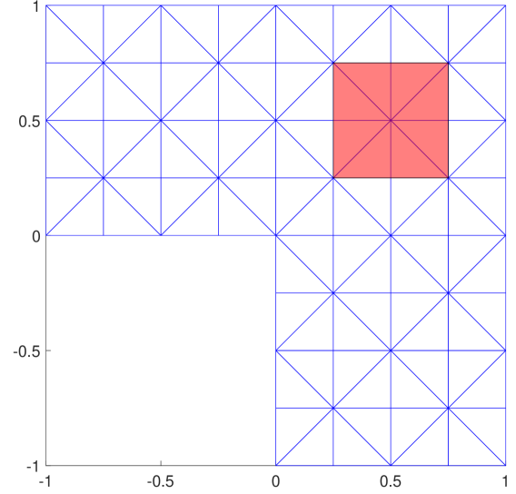
Setup 1

Setup 2

Setup 3

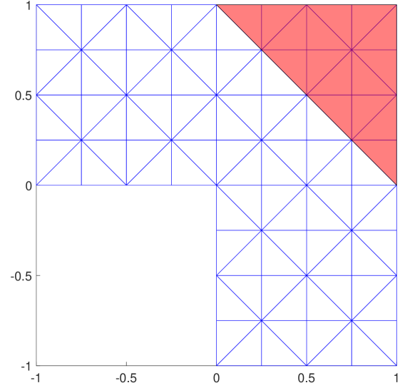
Setup 4

Figure 1. The supports of spatial features and initial meshes for all four setups.

Setup 2: estimation of pointwise values. Let $D_{\delta}=(-1,1)^{2}\setminus\overline{T}_{\delta}$, where $T_{\delta}$ is the triangle with vertices $(0,0)$, $(-1,\delta)$, and $(-1,-\delta)$. In this test case, we consider the spatial slit domain $D=(-1,1)^{2}\setminus([-1,0]\times\{0\})$. While the slit domain is not Lipschitz, it is well known that an elliptic problem on this domain can be seen as the limit of the problems posed on Lipschitz domains $D_{\delta}$ as $\delta\to 0$. Therefore, for this setup, we will perform computations on the domain $D=D_{\delta}$ with $\delta=0.005$. Aiming to approximate the expectation of a pointwise value of the solution $u$ to problem (1), we consider the following linear goal functional:

$$\mathscr{Q}(u)=\int_{\Gamma}\int_{D}q(x)u(x,\bm{y})\mathrm{d}x\,\mathrm{d}\pi(\bm{y}),$$

where the weight function $q\in L^{\infty}(D)$ is a mollifier centered at the point $x_{0}=(0.4,-0.5)\in D$ with radius $r=0.15$ (we refer to equation (58) in [5] for the specific expression for the function $q(x)$). The support of $q(x)$ and the initial mesh on $D$ are depicted in Figure 1. In this setup, we consider a nonaffine parametric diffusion coefficient and the constant right-hand side function; specifically, we set $a(x,\bm{y})=\exp(h(x,\bm{y}))$ and $f(x)\equiv 1$.

Setup 3: second moment of a linear goal functional. In this test case, we set the spatial domain to be the unit square $D=(0,1)^{2}$, and we consider again the affine-parametric diffusion coefficient, i.e., $a(x,\bm{y})=h(x,\bm{y})$. Furthermore, we follow [24, 5] and choose the forcing term in (1) so that the functional on the right-hand side of (5) is given by

$$\mathscr{F}(v)=-\int_{\Gamma}\int_{D}(\chi_{T_{f}},0)\cdot\nabla v(x,\bm{y})\mathrm{d}x\,\mathrm{d}\pi(\bm{y})=-\int_{\Gamma}\int_{T_{f}}\frac{\partial v}{\partial x_{1}}(x,\bm{y})\mathrm{d}x\,\mathrm{d}\pi(\bm{y})\ \,\forall\,v\in\mathscr{V};$$ (52)

here $\chi_{T_{f}}:D\to\{0,1\}$ is the characteristic function of the triangle $T_{f}\subset D$ with vertices $(0,0)$, $(0.5,0)$, and $(0,0.5)$. We consider a nonlinear goal functional given by the (scaled) second moment of a linear quantity of interest. Specifically, we define

$$\mathscr{Q}(u)=100\int_{\Gamma}\left(\int_{D}q(x)u(x,\bm{y})\,\mathrm{d}x\right)^{2}\mathrm{d}\pi(\bm{y}),$$ (53)

where $q(x)=\chi_{T_{q}}/|T_{q}|$, $\chi_{T_{q}}:D\to\{0,1\}$ is the characteristic function of the triangle $T_{q}$ with vertices $(0.5,1)$, $(1,0.5)$, and $(1,1)$. The motivation behind the representation for $\mathscr{F}(v)$ in (52) is to introduce non-geometric singularities into the solution to the primal problem, so that the primal and the dual solutions exhibit singular behavior in two different regions of the computational domain. Figure 1 shows the initial mesh on $D$ as well as the triangular subdomains $T_{f}$ (magenta) and $T_{q}$ (red).

In order to calculate $\mathscr{Q}(u_{\bullet}^{\rm SC})$, we proceed as follows:

$$\frac{\mathscr{Q}(u_{\bullet}^{\rm SC})}{100} =\int_{\Gamma}\bigg{(}\int_{D}q(x)u_{\bullet}^{\rm SC}(x,\bm{y})\,\mathrm{d}x\bigg{)}^{2}\,\mathrm{d}\pi(\bm{y})$$

$$=\int_{\Gamma}\bigg{(}\int_{D}q(x)\sum_{\bar{\bm{y}}\in\mathcal{Y}_{\bullet}}u_{\bullet\bar{\bm{y}}}(x)L_{\bullet\bar{\bm{y}}}(\bm{y})\,\mathrm{d}x\bigg{)}\,\bigg{(}\int_{D}q(x)\sum_{\bar{\bm{y}}^{\prime}\in\mathcal{Y}_{\bullet}}u_{\bullet\bar{\bm{y}}^{\prime}}(x)L_{\bullet\bar{\bm{y}}^{\prime}}(\bm{y})\,\mathrm{d}x\bigg{)}\,\mathrm{d}\pi(\bm{y})$$

$$=\sum_{\bar{\bm{y}},\bar{\bm{y}}^{\prime}\in\mathcal{Y}_{\bullet}}\int_{D}q(x)u_{\bullet\bar{\bm{y}}}(x)\,\mathrm{d}x\int_{D}q(x)u_{\bullet\bar{\bm{y}}^{\prime}}(x)\,\mathrm{d}x\int_{\Gamma}L_{\bullet\bar{\bm{y}}}(\bm{y})L_{\bullet\bar{\bm{y}}^{\prime}}(\bm{y})\,\mathrm{d}\pi(\bm{y}).$$

The integrals over the parameter domain $\Gamma$ are calculated as explained in §4.3. The spatial integrals are evaluated in a standard way by representing the samplewise finite element approximations as, e.g., $u_{\bullet\bar{\bm{y}}}(x)=\sum_{\xi\in\mathcal{N}_{\bullet}}c_{\bullet\bar{\bm{y}},\xi}\varphi_{\bullet,\xi}(x)$ and calculating the $q(x)$-weighted spatial integrals of the finite element basis functions $\varphi_{\bullet,\xi}(x)$.

2

Figure 2. Evolution of the goal-oriented error estimates (magenta lines) as well as the reference errors for uncorrected (blue lines) and corrected (red lines) approximations of $\mathscr{Q}(u)$ for setups 1 and 2.

3

Figure 3. Evolution of the goal-oriented error estimates (magenta lines) as well as the reference errors for uncorrected (blue lines) and corrected (red lines) approximations of $\mathscr{Q}(u)$ for setups 3 and 4.

Setup 4: expectation of a nonlinear convection term. Here, as in the first test case, we consider the model problem on the L-shaped domain $D=(-1,1)^{2}\setminus(-1,0]^{2}$ and set $f(x)\equiv 1$. We consider a nonaffine parametric coefficient $a(x,\bm{y})=\exp(h(x,y))$ and define the goal functional as the expectation of a nonlinear convection term, i.e.,

$$\mathscr{Q}(u)=\int_{\Gamma}\int_{D}q(x)u(x,\bm{y})\left(\frac{\partial u}{\partial x_{1}}(x,\bm{y})+\frac{\partial u}{\partial x_{2}}(x,\bm{y})\right)\;\mathrm{d}x\;\mathrm{d}\pi(\bm{y}),$$

where $q(x)=\chi_{T}/|T|$ and $\chi_{T}:D\to\{0,1\}$ is the characteristic function of the triangle $T\,{\subset}\,D$ with vertices $(0,1)$, $(1,0)$, $(1,1)$; see Figure 1 that also shows the initial mesh on $D$.

In order to evaluate $\mathscr{Q}(u_{\bullet}^{\rm SC})$, we use the following formula:

$$\mathscr{Q}(u_{\bullet}^{\rm SC}) =\int_{\Gamma}\int_{D}q(x)u_{\bullet}^{\rm SC}(x,\bm{y})\bigg{(}\frac{\partial u_{\bullet}^{\rm SC}}{\partial x_{1}}(x,\bm{y})+\frac{\partial u_{\bullet}^{\rm SC}}{\partial x_{2}}(x,\bm{y})\bigg{)}\,\mathrm{d}x\,\mathrm{d}\pi(\bm{y})$$

$$=\int_{\Gamma}\int_{D}q(x)\bigg{[}\sum_{\bar{\bm{y}}\in\mathcal{Y}_{\bullet}}u_{\bullet\bar{\bm{y}}}(x)L_{\bullet\bar{\bm{y}}}(\bm{y})\bigg{]}\sum_{\bar{\bm{y}}^{\prime}\in\mathcal{Y}_{\bullet}}\bigg{(}\frac{\partial u_{\bullet\bar{\bm{y}}^{\prime}}}{\partial x_{1}}(x)+\frac{\partial u_{\bullet\bar{\bm{y}}^{\prime}}}{\partial x_{2}}(x)\bigg{)}L_{\bullet\bar{\bm{y}}^{\prime}}(\bm{y})\,\mathrm{d}x\,\mathrm{d}\pi(\bm{y})$$

$$=\sum_{\bar{\bm{y}},\bar{\bm{y}}^{\prime}\in\mathcal{Y}_{\bullet}}\int_{D}q(x)u_{\bullet\bar{\bm{y}}}(x)\bigg{(}\frac{\partial u_{\bullet\bar{\bm{y}}^{\prime}}}{\partial x_{1}}(x)+\frac{\partial u_{\bullet\bar{\bm{y}}^{\prime}}}{\partial x_{2}}(x)\bigg{)}\,\mathrm{d}x\int_{\Gamma}L_{\bullet\bar{\bm{y}}}(\bm{y})L_{\bullet\bar{\bm{y}}^{\prime}}(\bm{y})\,\mathrm{d}\pi(\bm{y}).$$

Here, the computation of integrals over the parameter domain $\Gamma$ follows again the procedure described in §4.3, whereas the spatial integrals can be seen as bilinear forms. Thus, we evaluate these spatial integrals as matrix-vector products $\mathbf{c}_{\bullet\bar{\bm{y}}}^{\sf T}{\mathbf{B}}_{\bullet}\mathbf{c}_{\bullet\bar{\bm{y}}^{\prime}}$, where $\mathbf{c}_{\bullet\bar{\bm{y}}},\,\mathbf{c}_{\bullet\bar{\bm{y}}^{\prime}}$ are the coefficient vectors for Galerkin approximations $u_{\bullet\bar{\bm{y}}},\,u_{\bullet\bar{\bm{y}}^{\prime}}$ and $[{\mathbf{B}}_{\bullet}]_{\xi,\eta\in\mathcal{N}_{\bullet}}=\int_{D}q(x)\varphi_{\bullet,\xi}(x)\big{(}\frac{\partial\varphi_{\bullet,\eta}}{\partial x_{1}}(x)+\frac{\partial\varphi_{\bullet,\eta}}{\partial x_{2}}(x)\big{)}\,\mathrm{d}x$ (note that, at a given iteration of the algorithm, the matrix ${\mathbf{B}}_{\bullet}$ is the same for all collocation points).

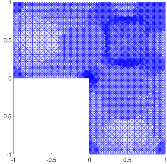
Setup 1 ($\mathcal{T}_{32}$)

Setup 2 ($\mathcal{T}_{30}$)

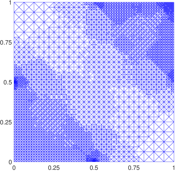
Setup 3 ($\mathcal{T}_{30}$)

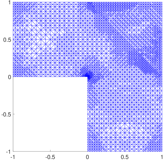
Setup 4 ($\mathcal{T}_{27}$)

Figure 4. Adaptively refined meshes for all four setups.

In Figures 2 and 3, for all setups, we plot the goal-oriented error estimates given by the right-hand sides of (30) and (44), respectively, as well as the reference errors for uncorrected and corrected approximations of $\mathscr{Q}(u)$ versus the number of degrees of freedom (dof) at each iteration of Algorithm 1. The reference value $\mathscr{Q}(u_{{\rm ref}})$ is calculated using the reference solution $u_{\rm ref}$ to the corresponding test problem. The reference solution for each setup is computed as a SC-FEM approximation using a large set of collocation points (generated by the union of the final index set $\Lambda_{\ell_{*}}$ and its full margin ${\rm K}(\Lambda_{\ell_{*}})$) and the second-order (P2) FEM on the uniform refinement of the final mesh $\mathcal{T}_{\ell_{*}}$ generated by the adaptive algorithm for the corresponding test problem. The plots show that in each setup the adaptive algorithm drives the goal-oriented error estimates (magenta lines) to zero. Moreover, these error estimates and the reference errors in the corrected approximation of $\mathscr{Q}(u)$ decay with the rate $O(\text{dof}^{-2/3})$. As expected, this is twice the rate of decay of the error in adaptive SC-FEM approximations of the primal solution, cf. [9, section 5]. In addition, the introduction of the correction term in (29) has a stabilizing effect on the decay of the corresponding reference error. Indeed, for each setup, the reference errors for corrected approximations of the goal functional (red lines in Figures 2, 3) decay monotonically (with exception of maybe a few initial iterations) and do so with the same rate as the goal-oriented error estimates. In contrast, the reference errors for uncorrected approximations (blue lines in Figures 2, 3) either exhibit jumps (in setups 1 and 3) or deviate from the decay rate of the goal-oriented error estimates (in setups 2 and 4).

We note that the gap between the red and magenta lines (that reflects the size of effectivity indices for the goal-oriented error estimation) for nonlinear goal functionals in Figure 3 is much wider than that for linear goal functionals in Figure 2. Specifically, the average effectivity index (i.e., the ratio of the error estimate to the reference error for the corrected approximation of the goal functional) is 7.1 in setup 1, 2.4 in setup 2, 100.2 in setup 3, and 16.2 in setup 4. Larger effectivity indices in the case of nonlinear goal functionals are likely due to the size of the constant $C_{\rm goal}$ in assumption (41) that affects the (hidden) constant in the goal-oriented error estimate (44).

Figure 4 depicts locally refined finite element meshes generated at intermediate iterations of the adaptive algorithm. This figure shows that for all setups the algorithm refines the finite element mesh according to spatial features in both the primal and the dual solution. These include corner singularities, local features due to a spatial subdomain in the definition of the goal functional (cf. Figure 1) and, in setup 3, non-geometric singularities induced by the choice of the forcing term $f$ in the primal problem.

7. Concluding remarks

Surrogate approximations of solutions to PDEs with uncertain inputs play an important role in reliable uncertainty quantification. They can be cheaply evaluated at any point in the parameter domain and are used to estimate a wide range of QoIs, thus, providing an effective alternative to Monte Carlo simulations. While being effective in approximating the input-output map and QoIs, surrogate approximations introduce numerical errors that need to be estimated and controlled in the course of simulations. In this work, we have proved reliable a posteriori estimates for the errors associated with computing QoIs in the SC-FEM context. Furthermore, we have designed a goal-oriented adaptive algorithm for reducing these errors. The numerical experiments presented in this paper and more extensive experiments included in [27] demonstrate the robustness of our error estimation strategy and the effectiveness of the adaptive algorithm. In particular, our conclusions hold for PDE problems with affine or nonaffine parametrizations of uncertainty in PDE inputs and for a range of QoIs represented by linear or nonlinear goal functionals.

Adaptive algorithms for the sparse grid-based SC-FEM are particularly effective when combined with dimensionality reduction techniques (see e.g., [14, 21]) and/or dimension adaptivity (see e.g., [13, 18]). The application of these techniques within the goal-oriented adaptive framework proposed in our work is currently being investigated and will be the subject of a future publication.

References

- [1] R. C. Almeida and J. T. Oden, Solution verification, goal-oriented adaptive methods for stochastic advection–diffusion problems, Comput. Methods Appl. Mech. Engrg., 199 (2010), pp. 2472–2486.
- [2] I. Babuška, F. Nobile, and R. Tempone, A stochastic collocation method for elliptic partial differential equations with random input data, SIAM J. Numer. Anal., 45 (2007), pp. 1005–1034.
- [3] R. Becker, E. Estecahandy, and D. Trujillo, Weighted marking for goal-oriented adaptive finite element methods, SIAM J. Numer. Anal., 49 (2011), pp. 2451–2469.
- [4] R. Becker and R. Rannacher, An optimal control approach to a posteriori error estimation in finite element methods, Acta Numer., 10 (2001), pp. 1–102.
- [5] A. Bespalov, D. Praetorius, L. Rocchi, and M. Ruggeri, Goal-oriented error estimation and adaptivity for elliptic PDEs with parametric or uncertain inputs, Comput. Methods Appl. Mech. Engrg., 345 (2019), pp. 951–982.
- [6] A. Bespalov, D. Praetorius, and M. Ruggeri, Goal-oriented adaptivity for multilevel stochastic Galerkin FEM with nonlinear goal functionals. Preprint, arXiv:2208.09388 [math.NA], 2023.
- [7] A. Bespalov and D. Silvester, Error estimation and adaptivity for stochastic collocation finite elements Part II: Multilevel approximation, SIAM J. Sci. Comput., 45 (2023), pp. A784–A800.
- [8] A. Bespalov, D. Silvester, and F. Xu, Adaptive ML-SCFEM, January 2023. Available online at https://github.com/albespalov/Adaptive_ML-SCFEM.
- [9] A. Bespalov, D. J. Silvester, and F. Xu, Error estimation and adaptivity for stochastic collocation finite elements Part I: Single-level approximation, SIAM J. Sci. Comput., 44 (2022), pp. A3393–A3412.
- [10] C. Bryant, S. Prudhomme, and T. Wildey, Error decomposition and adaptivity for response surface approximations from PDEs with parametric uncertainty, SIAM/ASA J. Uncertain. Quantif., 3 (2015), pp. 1020–1045.
- [11] T. Butler, C. Dawson, and T. Wildey, A posteriori error analysis of stochastic differential equations using polynomial chaos expansions, SIAM J. Sci. Comput., 33 (2011), pp. 1267–1291.
- [12] K. Eriksson, D. Estep, P. Hansbo, and C. Johnson, Introduction to adaptive methods for differential equations, Acta Numer., 4 (1995), pp. 105–158.
- [13] I.-G. Farcaş, T. Görler, H.-J. Bungartz, F. Jenko, and T. Neckel, Sensitivity-driven adaptive sparse stochastic approximations in plasma microinstability analysis, J. Comput. Phys., 410 (2020), pp. 109394, 24.
- [14] I.-G. Farcaş, P. C. Sârbu, H.-J. Bungartz, T. Neckel, and B. Uekermann, Multilevel adaptive stochastic collocation with dimensionality reduction, in Sparse grids and applications—Miami 2016, vol. 123 of Lect. Notes Comput. Sci. Eng., Springer, Cham, 2018, pp. 43–68.
- [15] M. Feischl, D. Praetorius, and K. van der Zee, An abstract analysis of optimal goal-oriented adaptivity, SIAM J. Numer. Anal., 54 (2016), pp. 1423–1448.
- [16] M. Feischl and A. Scaglioni, Convergence of adaptive stochastic collocation with finite elements, Comput. Math. Appl., 98 (2021), pp. 139–156.
- [17] M. B. Giles and E. Süli, Adjoint methods for PDEs: a posteriori error analysis and postprocessing by duality, Acta Numer., 11 (2002), pp. 145–236.
- [18] M. Griebel and U. Seidler, A dimension-adaptive combination technique for uncertainty quantification, Int. J. Uncertain. Quantif., 14 (2024), pp. 21–43.
- [19] D. Guignard and F. Nobile, A posteriori error estimation for the stochastic collocation finite element method, SIAM J. Numer. Anal., 56 (2018), pp. 3121–3143.
- [20] M. Karkulik, D. Pavlicek, and D. Praetorius, On 2D newest vertex bisection: Optimality of mesh-closure and -stability of -projection, Constr. Approx., 38 (2013), pp. 213–234.
- [21] J. Konrad, I.-G. Farcaş, B. Peherstorfer, A. Di Siena, F. Jenko, T. Neckel, and H.-J. Bungartz, Data-driven low-fidelity models for multi-fidelity Monte Carlo sampling in plasma micro-turbulence analysis, J. Comput. Phys., 451 (2022), pp. 110898, 20.
- [22] J. Lang, R. Scheichl, and D. Silvester, A fully adaptive multilevel stochastic collocation strategy for solving elliptic PDEs with random data, J. Comput. Phys., 419 (2020), pp. 109692, 17.
- [23] L. Mathelin and O. Le Ma\̂bm{i}tre, Dual-based a posteriori error estimate for stochastic finite element methods, Comm. App. Math. Com. Sc., 2 (2007), pp. 83–115.
- [24] M. S. Mommer and R. Stevenson, A goal-oriented adaptive finite element method with convergence rates, SIAM J. Numer. Anal., 47 (2009), pp. 861–886.
- [25] F. Nobile, R. Tempone, and C. G. Webster, A sparse grid stochastic collocation method for partial differential equations with random input data, SIAM J. Numer. Anal., 46 (2008), pp. 2309–2345.
- [26] S. Prudhomme and J. T. Oden, On goal-oriented error estimation for elliptic problems: application to the control of pointwise errors, Comput. Methods Appl. Mech. Engrg., 176 (1999), pp. 313–331.
- [27] T. Round, Goal-oriented adaptive algorithms for stochastic collocation finite element methods. PhD Thesis, University of Birmingham, 2024.
- [28] R. Stevenson, The completion of locally refined simplicial partitions created by bisection, Math. Comp., 77 (2008), pp. 227–241.