Optimizing Automatic Differentiation
with Deep Reinforcement Learning

Abstract

Computing Jacobians with automatic differentiation is ubiquitous in many scientific domains such as machine learning, computational fluid dynamics, robotics and finance. Even small savings in the number of computations or memory usage in Jacobian computations can already incur massive savings in energy consumption and runtime. While there exist many methods that allow for such savings, they generally trade computational efficiency for approximations of the exact Jacobian. In this paper, we present a novel method to optimize the number of necessary multiplications for Jacobian computation by leveraging deep reinforcement learning (RL) and a concept called cross-country elimination while still computing the exact Jacobian. Cross-country elimination is a framework for automatic differentiation that phrases Jacobian accumulation as ordered elimination of all vertices on the computational graph where every elimination incurs a certain computational cost. We formulate the search for the optimal elimination order that minimizes the number of necessary multiplications as a single player game which is played by an RL agent. We demonstrate that this method achieves up to 33% improvements over state-of-the-art methods on several relevant tasks taken from diverse domains. Furthermore, we show that these theoretical gains translate into actual runtime improvements by providing a cross-country elimination interpreter in JAX that can efficiently execute the obtained elimination orders.

1 Introduction

Automatic Differentiation (AD) is widely utilized for computing gradients and Jacobians across diverse domains including machine learning (ML), computational fluid dynamics (CFD), robotics, differential rendering, and finance (Baydin et al., 2018; Margossian, 2018; Forth et al., 2004a; Tadjouddine et al., 2002b; Giftthaler et al., 2017; Kato et al., 2020; Schmidt et al., 2022; Capriotti and Giles, 2011; Savine and Andreasen, 2021). To many researchers in the machine learning community, AD is synonymous with the backpropagation algorithm (Linnainmaa, 1976; Schmidhuber, 2014). However, backpropagation is just one particular way of algorithmically computing the Jacobian that is very efficient in terms of computations for “funnel-like” functions, i.e. with many inputs and a single scalar output such as in neural networks. In many other domains, we may find functions that do not have this particular property and thus backpropagation might not be optimal for computing the respective Jacobian (Albrecht et al., 2003; Capriotti and Giles, 2011; Naumann, 2020). In fact, there exists a wide variety of AD algorithms, each of them coming with its own advantages and drawbacks regarding computational cost and memory consumption depending on the function they are applied to. Many of these AD algorithms can be viewed as special cases of cross-country elimination (Griewank and Walther, 2008). Cross-County Elimination frames AD as an ordered vertex elimination problem on the computational graph with the goal of reducing the required number of multiplications and additions. However, finding the optimal elimination procedure is a NP-complete problem (Naumann, 2008). Inspired by recent advances in finding optimal matrix-multiplication and sorting algorithms (Fawzi et al., 2022; Mankowitz et al., 2023), we demonstrate that deep RL successfully finds efficient elimination orders which translate into new automatic differentiation algorithms and practical runtime gains (Figure 1). Cross-country elimination is particularly amenable for automatization since it provably yields the exact Jacobian for every elimination order. The solution we seek thus reduces to only finding a optimal elimination order, without the need to evaluate the quality of Jacobian approximations (such as in Neural Architecture Search). An important body of prior work aimed to find more efficient elimination techniques through heuristics, simulated annealing or dynamic programming and minimizing related quantities such as fill-in (Naumann, 1999, 2020). However, none of these works was successful in optimizing with respect to relevant quantities such as number of multiplications or memory consumption. We set up our optimization problem by formulating cross-country elimination as a single player RL game called VertexGame. At each step of VertexGame, the agent selects a vertex to eliminate from the computational graph according to a certain scheme called vertex elimination. At each step, the reward is equal to the negative of the number of multiplications incurred by the particular choice of vertex. VertexGame is played by an AlphaZero-based agent (Silver et al., 2017; Schrittwieser et al., 2019; Danihelka et al., 2022) with policy and value functions modeled with a transformer architecture that processes the graph representation and predicts the next vertex to eliminate, thereby incrementally building the AD algorithm.
Our approach discovers from scratch new vertex elimination orders, i.e. new AD algorithms that are tailored to specific functions and improve over the established methods such as minimal Markowitz degree. We further demonstrate the efficacy of the discovered algorithms on real world tasks by including Graphax, a novel sparse AD package which builds on JAX (Bradbury et al., 2018) and enables the user to differentiate Python code with cross-country elimination. Our main contributions are summarized as follows:

• We demonstrate that optimizing elimination order can be phrased as a reinforcement learning game by leveraging the graph view of AD,

• We show that a deep RL agent finds new, tailored AD algorithms that improve the state-of-the-art on several relevant tasks,

• We investigate how the discovered novel elimination procedures translate into actual runtime improvements by implementing Graphax, a cross-country elimination interpreter in JAX allowing the efficient execution of newly found elimination orders.

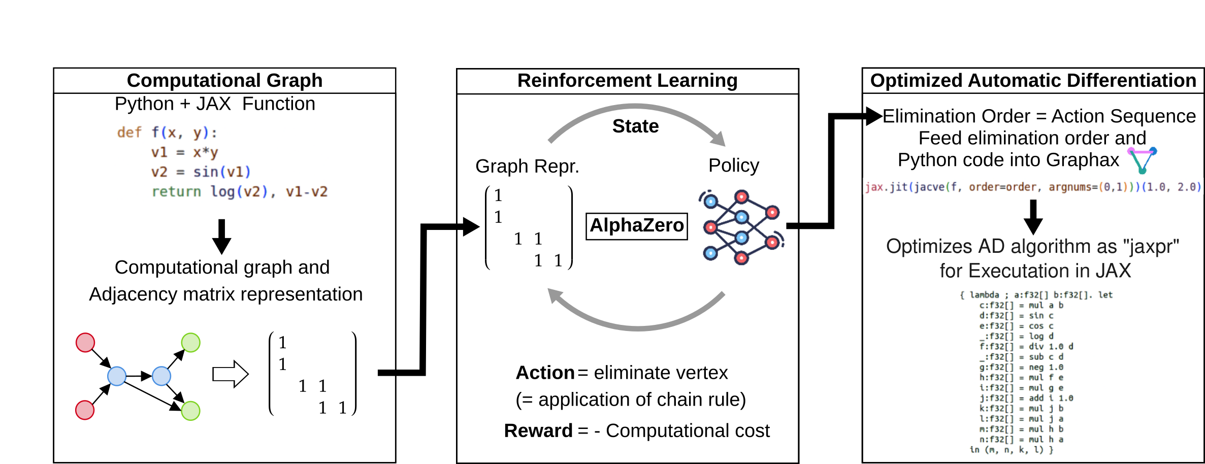
Figure 1: Summary of the AlphaGrad pipeline. We trained a neural network to produce new Automatic Differentiation (AD) algorithms using Deep RL that can be used in JAX. The resulting algorithms significantly outperform the current state of the art.

1.1 Related Work

RL for Algorithm Research: AlphaTensor and AlphaDev successfully demonstrated that model-based deep RL finds new and improved matrix-multiplication and sorting algorithms (Fawzi et al., 2022; Mankowitz et al., 2023). In particular, AlphaTensor used an extension of the AlphaZero RL agent to search for new matrix-multiplications algorithms that require fewer multiplication operations by directly using this quantity as a reward. The key insight is that different matrix-multiplication algorithms have a common, simple representation through the three-dimensional matrix-multiplication tensor which can be manipulated by taking different actions, resulting in algorithms of varying efficiency. Feeding this tensor into the RL agent, they successfully improved on matrix-multiplication algorithms for 4x4 matrices by beating Strassen’s algorithm, the current state-of-the-art, with an improvement from 49 to 47 necessary multiplications. In a similar vein, AlphaDev improved simple sorting algorithms by representing the sorting algorithm as a series of CPU instructions which then have to be arranged in the correct way to achieve the correct sorting output. Instead of using the number of CPU operations as an optimization target, the agent was trained on actual execution times. Our work follows in these footsteps by tackling the difficult problem of finding new and improved AD algorithms for arbitrary functions and hence we termed our method AlphaGrad.
RL for Compiler Optimization: A number of works have tackled the complex issue of optimizing the compilation of various computational graphs with deep RL. Knossos (Jinnai et al., 2019) leverages the A^∗ algorithm to optimize the compilation of simple neural networks. It employs a model to estimate computational cost and utilizes expression rewriting techniques to enhance performance. While Knossos is hardware agnostic, it needs to be trained from scratch for every new computational graph. GO and REGAL both improve on this shortcoming and generalize to new, unseen graphs at the cost of losing the hardware-agnostic property(Paliwal et al., 2019; Zhou et al., 2020). REGAL learns a graph neural network-based policy using a REINFORCE-based genetic algorithm to optimize the scheduling of the individual operations of a graph to the set of available devices, thereby successfully reducing peak memory usage for different deep learning workloads. Only GO is directly trained on actual wall time and handles all relevant optimizations jointly, including device placement, operation fusion and, operation scheduling. GO learns a policy based on graph neural networks and recurrent attention using PPO and successfully demonstrates improvements over Tensorflow’s default compilation strategy. While our work also makes use of the computational graph, the goal is to find novel AD algorithms instead of optimizing compilation itself, although these problems are related since the new AD algorithm is compiled before execution as well.
Optimization of AD While no prior work directly aims at improving AD with deep RL, several studies aimed at enhancing AD by other methods. The closest related work is (Naumann, 1999) where simulated annealing was applied to reduce the number of multiplications necessary for Jacobian accumulation. The algorithms struggled to significantly outperform state-of-the-art even when it was initialized with a reasonably good elimination order. In a similar manner, (Naumann, 2020) directly optimized the elimination order with dynamic programming albeit with respect to a different optimization target called fill-in on randomly generated graphs that do not necessary represent well-defined, executable functions. Our work directly optimizes for the number of multiplications required to accumulate the Jacobian on real-world problems. Another approach described in (Chen et al., 2012) utilized integer linear programming to find optimal elimination orders with respect to number of multiplications, but only dealt with very small problems with up to twenty intermediate vertices. Our approach successfully finds new AD algorithms from scratch for complex problems with hundreds of intermediate vertices.

2 Automatic Differentiation and Cross-Country Elimination

AD is a systematic approach to computing the derivatives of dependent variables $\mathbf{y}=f(\mathbf{x})\in\mathbb{R}^{m}$ with respect to the independent variables $\mathbf{x}\in\mathbb{R}^{n}$ utilizing the chain rule. AD enables the precise and efficient calculation of gradients, Jacobians, Hessians, and higher-order derivatives (Linnainmaa, 1976). Unlike methods that rely on finite differences or symbolic differentiation, AD offers a systematic way to compute derivatives up to machine precision, making it an indispensable tool in many numerical scientific problems and machine learning (Baydin et al., 2018; Griewank and Walther, 2008). AD leverages the fact that most computer programs can be broken down into a sequence of simple elemental operations, for example additions, multiplications and trigonometric functions. Partial derivatives of these elemental operations are coded into the AD software and the Jacobian is accumulated by recursively applying the chain rule to the evaluation procedure. Since the partial derivatives are known up to machine precision, AD gives the Jacobian up to machine precision.

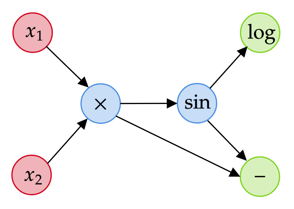
(a) Computational graph of $f(x_{1},x_{2}).$

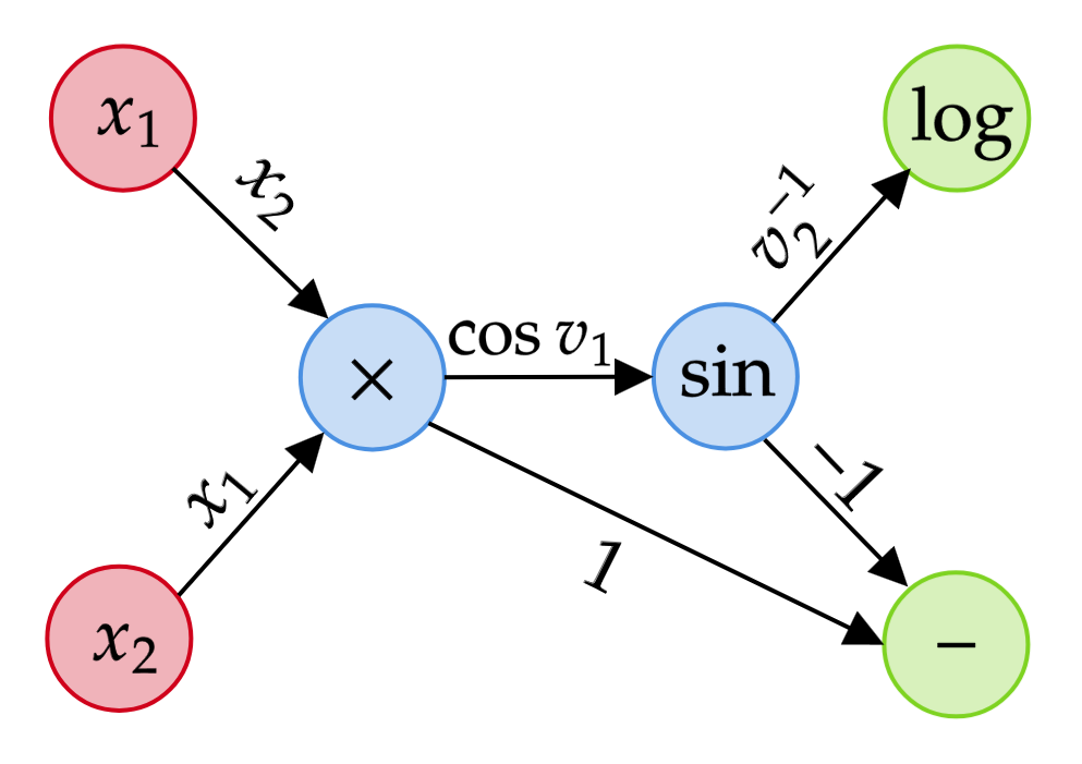
(b) Adding partial derivatives.

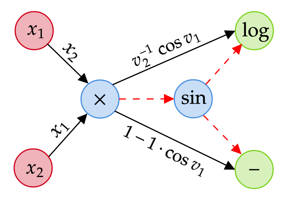
(c) Elimination of vertex 2.

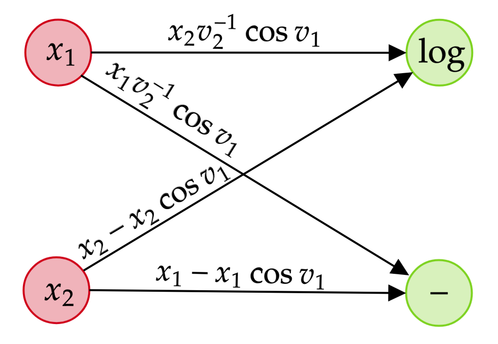
(d) Graph after eliminating vertex 1.

Figure 2: Step-by-step visual description of cross-country elimination with the simple example function $f(x_{1},x_{2})=(\log\sin(x_{1}x_{2}),x_{1}x_{2}-\sin(x_{1}x_{2}))^{\top}$. (2(a)) Initial computational graph. (2(b)) The partial derivatives are added to the edges of the computational graph. The intermediate variables $v_{1}$ and $v_{2}$ are defined through $v_{1}=x_{1}x_{2}$ and $v_{2}=\cos v_{1}$. (2(c)) Elimination of vertex 2 associated with the multiplication operation. The dotted red lines represent the edges that are deleted. (2(d)) Final bipartite graph after both intermediate vertices have been eliminated. All remaining edges contain entries of the Jacobian.

2.1 Graph View and Vertex Elimination

We take the graph view of AD where a function is defined through its computational graph 2(a) $\mathcal{G}=(V,E)$ with its vertices $\mathcal{V}$ being the elemental operations $\phi_{j}$ and directed edges $\mathcal{E}$ that describe the data dependencies between the operations. The relation $i\prec j$ states that vertex $i$ has an edge connecting it with vertex $j$, meaning that the output $v_{i}$ of $\phi_{i}$ is an input of $\phi_{j}$. The partial derivatives of the elemental operations with respect to their dependents are assigned to the connecting edges (see figure 2(b)). We can then identify the edges of the graph with their respective partial derivatives $c_{ij}=\frac{\partial\phi_{j}}{\partial v_{i}}$. The cross-country elimination algorithm computes the Jacobian by a procedure called vertex elimination.

Definition 1

(Griewank and Walther, 2008) For a computational graph $\mathcal{G}=(V,E)$ with partial derivatives $c_{ij}$, vertex elimination of vertex $j$ is defined as the update

$$c_{ik}\mathrel{+}=c_{ij}c_{jk}\ \forall(i,k)\in\mathcal{V}\times\mathcal{V}\ \mathrm{where}\ i\succ j\ \mathrm{and}\ j\prec k$$ (1)

and then setting $c_{ij}=c_{ik}=0$ for all involved vertices. The $\mathrel{+}=$ operator creates a new edge if there is no edge $c_{ik}$ and otherwise adds the new value to the existing value.

Intuitively, vertex elimination can be understood as the local application of the chain rule to a single vertex in the graph since the multiplication $c_{ij}c_{jk}$ is exactly the result of applying the chain rule to $(\phi_{j}\circ\phi_{k})(v_{i})$. If a vertex has multiple incoming and outgoing edges, all combinations of incoming and outgoing edges are resolved to create new edges. If an edge already exists, we add the result of the product to it, in accordance with the rules for total derivatives. After the new edges are added to the graph, we delete all edges connected to the eliminated vertex since all the derivative information is now contained in the new edges (see figure 2(c)). Note that the new graph resulting from a vertex elimination no longer directly represents the data dependencies of the function since the eliminated vertex is now disconnected.

2.2 Cross Country and Elimination Orders

The repeated application of the vertex elimination procedure to a computational graph (i.e. cross country elimination) until all intermediate vertices are eliminated will yield a graph where the input vertices and output vertices are directly connected by edges (no intermediate vertices left, see figure 2(d)). This is called a bipartite graph and the edges of this graph contain the components of the Jacobian. There is no restriction on the order in which the vertices are eliminated, but the choice will significantly influence computational cost and memory (Tadjouddine et al., 2006). In the graph view, computational cost is straightforward to measure since every vertex elimination incurs a known number of multiplications that depends on the shapes of the elemental Jacobians which can be used as a proxy for execution time. We can ignore the cost of evaluating the partial derivatives since they have to be performed regardless of the elimination order. Thus, we use the number of multiplications as the optimization target for the remainder of this work. The two most common choices for elimination orders are to either eliminate the vertices in the forward or reverse order. These two modes are called forward-mode AD and reverse-mode AD (backpropagation), respectively.
Forward-mode AD, where vertices are eliminated in the same order as the computational graph is traversed, is particularly efficient for functions where the number of input variables $n$ is much smaller than the number of output variables $m$, i.e. $n\ll m$. In contrast, reverse-mode AD traverses the graph in the opposite direction and is particularly suited for the cases where $n\gg m$. This is the case in machine learning and neural networks using scalar loss functions, which is why reverse-mode AD is the default choice in such workloads.

2.3 Minimal Markowitz Degree

A more advanced technique is to eliminate vertices with the lowest Markowitz degree first Griewank and Walther (2008). The Markowitz degree of a vertex is defined as the number of incoming vertices times the number of outgoing vertices, i.e. $\mathrm{Mark}(j)=|i\succ j||j\prec k|,$ where $|\cdot|$ denotes the cardinality of the set $\{i|i\succ j\}$. Thus the elimination order is constrained by finding the vertex with the lowest Markowitz degree first, eliminating it and then finding the next vertex with minimal Markowitz degree on the resulting graph. This elimination scheme is one of the best known heuristics for finding efficient elimination orders and can incur savings of up to 20% over forward- and reverse-mode AD (Albrecht et al., 2003; Griewank and Walther, 2008). However, for computational graphs that have many inputs and few outputs, it is often outperformed by reverse-mode AD.

2.4 Vector-valued Functions

In most applications, vector-valued functions are used as elemental building blocks of more complex applications. While in most cases, these vectorized operations could be broken down into scalar operations, this would be impractical since it would increase the size of the computational graph representation and action space by orders of magnitude. Thus, it is best to allow vertices of the computational graph to be vector-valued which results in the partial derivatives assigned to the edges becoming Jacobians in their own right. The multiplication operations during vertex elimination are then accordingly replaced with matrix multiplications or higher-order contractions of the elemental Jacobians. For many operations, the Jacobians themselves have a particular internal sparsity structure which can be exploited when performing the eliminations. Graphax is able to exploit the internal sparsity to accelerate the Jacobian computations. A simple example is the multiplication of a vector with a matrix followed by the application of a non-linear function $f(\mathbf{x},\mathbf{W})=\tanh{(\mathbf{W}\cdot\mathbf{x})}$. The input vertices are given by the input $\mathbf{x}$ and weights $\mathbf{W}$ and the intermediate vertex is matrix multiplication $a_{i}=\sum_{i}W_{ij}x_{j}$ with the partial derivatives

$$\dfrac{\partial a_{i}}{\partial W_{kl}}=x_{l}\delta_{ik}, \dfrac{\partial a_{i}}{\partial x_{k}}=W_{ki}.$$ (2)

The output vertex represents the application of the activation function $y_{i}=\tanh{a_{i}}$ with the partial derivative

$$\dfrac{\partial y_{i}}{\partial a_{j}}=\delta_{ij}(1-\tanh^{2}{a_{i}}).$$ (3)

According to the vertex elimination rule, upon elimination of the intermediate vertex the two Jacobians in equation (2) are assigned to the incoming edges are contracted together with the Jacobian from the outgoing edge in equation (3):

$$\dfrac{\partial y_{i}}{\partial W_{kl}}= \sum_{j}(1-\tanh^{2}{a_{i}})\delta_{ij}\delta_{jk}x_{l}=\delta_{ik}(1-\tanh^{2}{a_{i}})x_{l},$$ (4)

$$\dfrac{\partial y_{i}}{\partial x_{k}}= \sum_{j}(1-\tanh^{2}{a_{i}})\delta_{ij}W_{jk}=(1-\tanh^{2}{a_{i}})W_{ki}.$$ (5)

In both cases, instead of a matrix multiplication, one can perform simple element-wise multiplications as shown in figure 3(a). For vectorized cross-country elimination to be efficient, it is paramount to exploit this property. Current state-of-the-art AD frameworks typically lack the ability to perform cross-country elimination and subsequently can not deal with sparse Jacobians. The only exception the authors are aware of is EliAD, an AD interpreter in C++ which is fully capable of processing given elimination orders and create the derivative source code (Tadjouddine et al., 2002a). However, we developed Graphax as a novel AD interpreter that builds on Google’s JAX (Bradbury et al., 2018) in order to leverage it’s defining features such as JIT compilation, automated batching, device parallelism and a user-friendly Python front-end. Graphax is a fully fledged AD interpreter capable of performing cross-country elimination as described above and outperforms JAX’ AD on the relevant tasks by several orders of magnitude (see appendix B). Graphax and AlphaGrad are available under and https://github.com/jamielohoff/graphax and https://github.com/jamielohoff/alphagrad.

2.5 Computational Graph Representation and Network Architecture

We describe here how the computational graph is represented for optimization in the RL algorithm, as well as the network architecture that is optimized with AlphaZero.

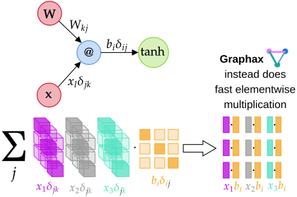
(a) Sparse vertex elimination.

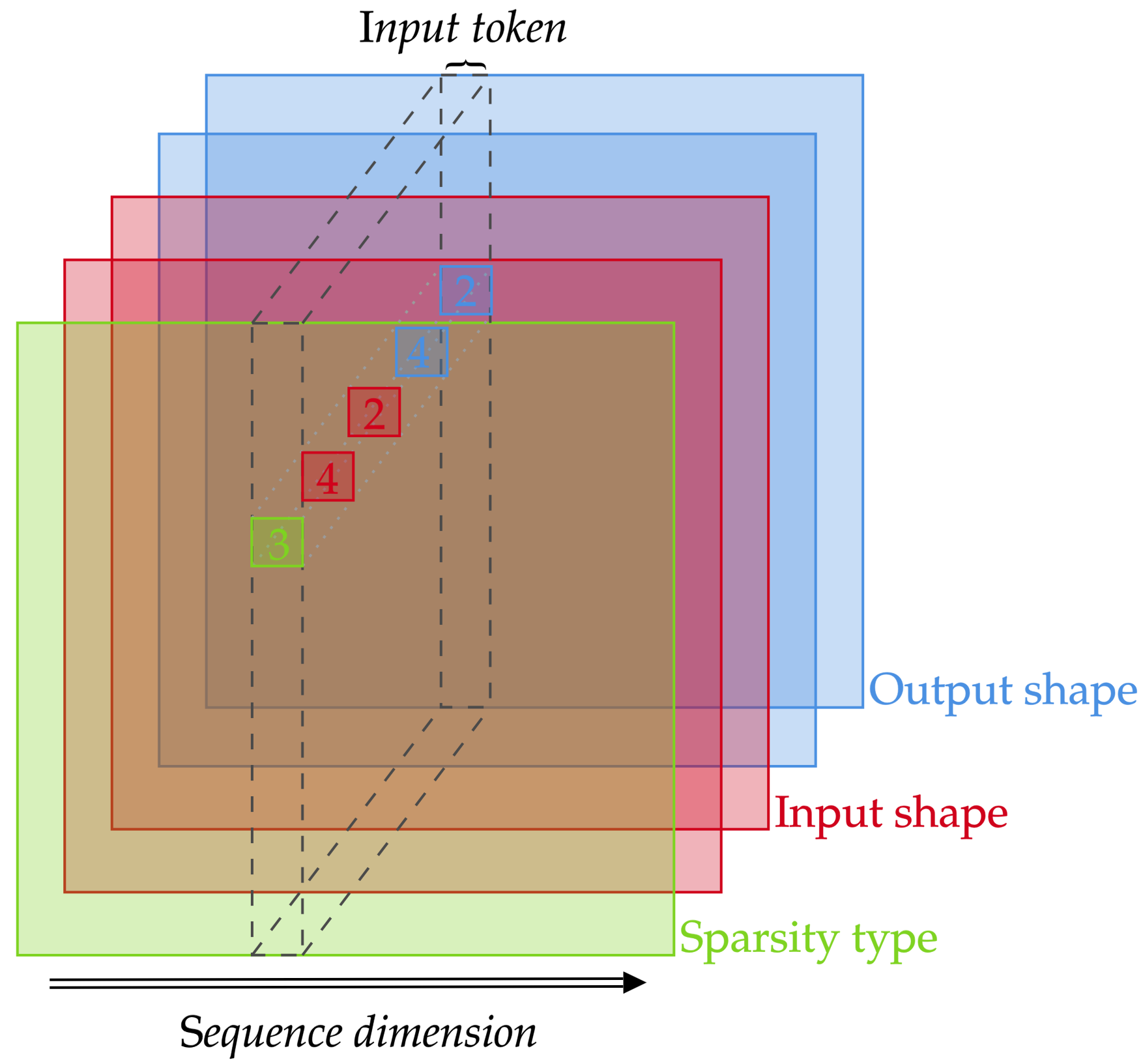
(b) Computational graph representation.

Figure 3: (3(a)) Graphax implements sparse vertex elimination to benefit from the advantages of cross country elimination. (3(b)) Sketch of the three-dimensional adjacency tensor that represents the computational graph. The colored surfaces represent the five different values encoded in the third dimension. The red and blue surfaces together contain the shape of the Jacobians while the green surface encodes their sparsity. The vertical dotted slices represent the input connectivity of a single vertex. In this work, we compress and feed the vertical slices as tokens into the transformer backbone such that we build a sequence running in direction of the black arrow.

In the scalar case, the computational graph can be represented by its adjacency matrix, meaning that for every pair of vertices $(i,j)$ that share an edge, we set the $i$-th row and the $j$-th column of the matrix to $1$. For the vectorized case, we define an extended adjacency tensor by extending the matrix into the third dimension. Along this third dimension, we store 5 values that describe the sparsity pattern and shape of the Jacobian associated with the respective edge. The first value is an integer between -10 and 10 which encodes the sparsity type of the Jacobian. Details about the supported sparsity types can be found in Appendix C. The next four values contain the shape of the Jacobian associated with the respective edge and thus imply that this representation can at most deal with Jacobians of the shape $\frac{\partial y_{ij}}{\partial x_{kl}}$ where the first two values describe the shape of $x_{kl}$ and the other two values describe the shape of $y_{ij}$. This can be expanded to arbitrary tensor sizes of $x$ and $y$, but then also requires the definition of new sparsity types to account for the additional dimensions. Figure 3(b) shows the representation of the entire computational graph and a single selected edge with a Jacobian of shape $(4,2,4,2)$ with sparsity type 3. A horizontal or vertical slice of the extended adjacency tensor gives the input or output connectivity of a particular vertex. These slices can be compressed and used as tokens to be fed into a transformer block network where they are processed simultaneously by the attention mechanism so that the model gets a full view of the graph’s connectivity. In this work, we compress vertical slices into tokens using a convolutional layer with kernel size (3, 5) and use a linear projection to create a 64-dimensional embedding. We found it helpful to apply a positional encoding to the tokens (Vaswani et al., 2017). The output of the transformer is then fed into a policy and a value head. The policy head is a MLP mapped across every token separately, thus creating a probability distribution over the vertices to determine the next one to be eliminated. Already eliminated vertices are masked. Similarly, the value head is also a MLP that predicts a score for every token. These scores are then summed to give the value prediction of the network.

3 Reinforcement Learning for Optimal Elimination Orders

Cross-country elimination is typically introduced as a means to reduce the computational cost of computing the Jacobian. We cast the problem of finding an efficient vertex elimination order as a single-player RL game called VertexGame. At every step of the game, the agent selects the next vertex to be eliminated by observing the current connectivity of the computational graph. Since it is hard to directly optimize for execution time, it is common to use the number of multiplications incurred by the elimination order as a proxy value (Tadjouddine et al., 2006, 2002b; Albrecht et al., 2003). Thus, we chose the negative number of multiplications incurred by eliminating the selected vertex as reward. We use action masking to prevent the agent from eliminating the same vertex twice. This also ensures that the accumulated Jacobian is always exact and has a clear terminal condition: when the extended computational graph is bipartite, the game ends.
Between elimination orders, the magnitude of the reward can range across multiple orders of magnitude. To tackle this, we rescale the cumulative reward using a monotonous function. For the functions with scalar inputs as well as RoeFlux_3d and random function $f$, we found the method presented in (Kapturowski et al., 2019) performed well, i.e. we scaled with $s(r)=\mathrm{sgn}(r)(\sqrt{|r|+1}-1)+\epsilon r$ where $\epsilon=10^{-3}$. For MLP and TransformerEncoder tasks, the best performance was achieved with logarithmic scaling $s(r)=\log r$ (Hafner et al., 2024). VertexGame is played by an AlphaZero agent, which successfully finds new AD algorithms. To reduce the computational cost of the AlphaZero agent (Silver et al., 2017), we employed the Gumbel AlphaZero agent Danihelka et al. (2022). Gumbel AlphaZero is a policy improvement algorithm based on sampling actions without replacement which utilizes the Gumbel softmax trick and other augmentations. This algorithm is guaranteed to improve the policy while significantly reducing the number of necessary Monte-Carlo Tree Search (MCTS) simulations. On most tasks, we found that 50 MCTS simulations were sufficient to reach satisfactory performance. Appendix D contains more details about the training of the agent.

4 Experiments

Table 1: Number of multiplications required by the best discovered elimination order for a batch size of one. Results obtained from VertexGame played by the AlphaZero agent with 50 MCTS simulations and a Gumbel noise scale of 1.0. $\dagger$ marks the experiments where we employed a $\log$-scaling of the cumulative reward instead of the default scaling. The values in parentheses were obtained for 250 MCTS simulations.

Task	Forward	Reverse	Markowitz	AlphaGrad
RoeFlux_1d	620	364	407	320
RobotArm_6DOF	397	301	288	231
HumanHeartDipole	240	172	194	149
PropaneCombustion	151	90	111	88
Random function $g$	632	566	451	417
BlackScholes	545	572	350	312
RoeFlux_3d	1556	979	938	811
Random function $f$	17728	9333	12083	6374
2-layer MLP†	10930	392	4796	398 (389)
Transformer†	135010	4688	51869	4831 (4656)

To demonstrate the effectiveness of our approach, we devised a set of tasks sampled from different scientific domains where AD is used to compute Jacobians. More details concerning the tasks are listed in appendix A.
Deep Learning is a prime example for the success of large-scale AD. We analyze a two-layer MLP with layer norm as described in (Goodfellow et al., 2016) and a small-scale version of the transformer encoder (Dosovitskiy et al., 2020).
Computational Fluid Dynamics relies on AD for computation of the flux Jacobian on the boundaries of the simulation grid cells. The RoeFlux is particularly relevant and has been studied extensively with vertex elimination in the past (Roe, 1981; Tadjouddine et al., 2002b; Zubair et al., 2023). We test on the 1D and the 3D variants of this problem.
Differential Kinematics uses Jacobians to quantify the behavior of a robot or other mechanical system with respect to their controllable parameters (e.g. joints, actuators). There has been a surge in interest of computing the Jacobian using AD(Giftthaler et al., 2017). We chose the forward kinematics of a 6-DOF robot arm as a representative problem and follow (Dikmenli, 2022) for the implementation.
Non-Linear Equation Solving requires the computation of large Jacobians to apply state-of-the-art solvers. The MINPACK problem collection provides a set of problems derived from real-life applications of non-linear optimization and designed to be representative of commonly encountered problems. In particular, we analyze the HumanHeartDiple and PropaneCombustion tasks, for which vertex elimination has also been analyzed thoroughly in (Forth et al., 2004b; Averick et al., 1992).
Computational Finance makes use of AD for fast computation of the so called “greeks” which measure the sensitivities of the value of an option to the model parameters(Naumann, 2010; Savine and Andreasen, 2021). Here, we compute the second-order greeks of the Black-Scholes equation using AD by computing the Hessian of the Black-Scholes equation through evaluation of the Jacobian of the Jacobian Black and Scholes (1973). This way, this task serves a two-fold purpose by also demonstrating how our approach is also useful for finding good AD algorithms for higher-order derivatives.
Random Functions are also commonly used to evaluate the performance of new AD algorithms (Albrecht et al., 2003). We generated two functions random functions $f$ and $g$ with vector-valued and only scalar inputs respectively. The random code generator used to generate these arbitrary functions is included in the accompanying software package.

4.1 Finding Optimal Elimination Orders

Table 1 shows the number of multiplications required by the best elimination order found over 6 runs with different seeds. The model was trained from scratch on each task separately with a batchsize of 1 to to keep the rewards as small as possible. The resulting AD algorithms are nonetheless scalable to arbitrary batchsizes. We use forward-mode, reverse-mode and the minimal Markowitz degree method as baselines for comparison. The first six tasks are simple functions with only scalar inputs and simple operations and the cumulative reward stays within the same order of magnitude, making them easier to solve. For all tasks, our approach was able find new elimination orders with improvements ranging from 2% to almost 20%. We found that even for only 5 MCTS simulations, the agent was able to find better than state-of-the-art solutions for the scalar tasks. On the opposite spectrum, our experiments with 250 MCTS simulations yielded no significant improvement over the results presented in table 1. The four remaining tasks are arguably more difficult since the vector-valued inputs and large variance within possible rewards provide an additional challenge. The RoeFlux_3d and random function $f$ were solved successfully with 50 MCTS simulations and yielded improvements of up to 33%. This is in stark contrast to prior work such as (Naumann, 1999), where algorithms such as simulated annealing or dynamic programming struggled to even beat common heuristics such as minimal Markowitz or reverse-mode AD.
With a budget of only 50 MCTS simulations, AlphaGrad failed to find improvements for both deep learning tasks. The authors conjecture that this is not only due to difficulties presented above but because reverse-mode AD (backpropagation) is already a very well-suited algorithm for computing Jacobians of “funnel-like” computational graphs with many inputs and a single, scalar output. Despite this, with an increase to 250 MCTS simulations, the agent marginally outperformed backpropagation for both deep learning models. Appendix E contains more information about the experiments, including reward curves, the actual elimination orders and more details about their implementation. We also include joint training runs where the agent was trained on all tasks at once. While the results were inferior to the separate training mode, the agent found new elimination orders for almost all tasks except the MLP, TransformerEncoder, RoeFlux_3d and PropaneCombustion tasks. For the random function $f$ and BlackScholes_Jacobian task, the agent outperformed the results in table 1 with new best results of 5884 and 307 respectively, thereby showing that the algorithm search might benefit from training on diverse tasks simultaneously. This also hints at the possibility of building a more general statistical model of AD applicable workloads from many different domains. We also experimented with PPO as an alternative for the AlphaZero agent (see appendix F).

Table 2: Median runtimes for the results obtained in table 1. Results were measured with Graphax for batchsize 512 on an AMD EPYC 9684X 2x96-Core processor. Uncertainties are given as 2.5- and 97.5-percentiles over 1000 trials. Execution time is given in milliseconds and default XLA compilation flags were used for all experiments. The size of the networks, i.e. the number of neurons were increased for the MLP and Transformer Encoder by a factor of 16 to create a more realistic sample. GPU experiments were run on a NVIDIA RTX 4090.

Task	Forward	Reverse	Markowitz	AlphaGrad
RoeFlux_1d	$3.03_{-0.27}^{+0.17}$	$3.08_{-0.23}^{+0.17}$	$2.87_{-0.66}^{+0.22}$	$2.19_{-0.35}^{+0.30}$
RobotArm_6DOF	$8.85_{-0.17}^{+0.21}$	$8.48_{-0.20}^{+0.32}$	$8.55_{-0.36}^{+0.38}$	$6.05_{-0.35}^{+0.34}$
HumanHeartDipole	$16.97_{-2.39}^{+1.23}$	$16.87_{-3.90}^{+1.45}$	$16.42_{-2.73}^{+1.29}$	$15.94_{-1.10}^{+1.11}$
PropaneCombustion	$36.91_{-1.50}^{+2.87}$	$36.47_{-0.51}^{+1.45}$	$36.99_{-1.11}^{+1.55}$	$36.45_{-1.31}^{+2.47}$
Random function $g$	$82.41_{-2.97}^{+2.85}$	$81.64_{-3.56}^{+2.82}$	$82.97_{-1.17}^{+1.38}$	$80.56_{-2.30}^{+1.61}$
BlackScholes	$5.04_{-0.33}^{+0.23}$	$5.02_{-0.39}^{+0.30}$	$5.03_{-0.29}^{+0.23}$	$4.77_{-0.29}^{+0.23}$
RoeFlux_3d	$72.26_{-6.02}^{+3.22}$	$83.98_{-6.68}^{+5.69}$	$91.27_{-16.49}^{+11.59}$	$63.92_{-5.76}^{+4.45}$
Random function $f$	$12.42_{-0.25}^{+0.66}$	$11.54_{-0.27}^{+0.15}$	$20.20_{-0.31}^{+0.26}$	$9.12_{-0.06}^{+0.08}$
2-layer MLP†	$760.63_{-53.30}^{+80.01}$	$29.67_{-4.05}^{+1.33}$	$317.65_{-19.34}^{+53.30}$	$28.73_{-3.78}^{+1.32}$
2-layer MLP†(GPU)	$11.04_{-0.13}^{+0.31}$	$0.30_{-0.03}^{+0.02}$	$1.01_{-0.05}^{+0.02}$	$0.29_{-0.03}^{+0.02}$
Transformer†	$990.09_{-31.11}^{+35.42}$	$39.07_{-7.67}^{+4.59}$	$498.94_{-19.62}^{+20.34}$	$40.38_{-3.62}^{+5.26}$
Transformer†(GPU)	$21.38_{-0.06}^{+0.22}$	$0.29_{-0.03}^{+0.02}$	$16.17_{-0.09}^{+15.04}$	$0.28_{-0.01}^{+0.02}$

4.2 Runtime Improvements and the Graphax library

The results in table 2 are mainly of theoretical value. Here, we investigate how these translate into actual runtime improvements. For this purpose, we implemented Graphax, to our knowledge the first Python-based AD interpreter able to leverage cross-country elimination. Graphax builds a second program that computes the Jacobian by leveraging the elimination orders found by AlphaGrad and using the source code of the function as a template by analyzing its Jaxpression. The Jaxpression is JAX’ own representation of the computational graph of the function in question. Table 2 shows runtime improvements for the elimination orders found in table 1 for a batchsize of 512 with varying levels of improvement. This is due to the fact that the number of multiplications alone was only a proxy to capture the complexity of the entire program. It ignores other relevant quantities such as memory accesses and operation fusion during compilation. Nonetheless, a particularly impressive gain over the state-of-the-art methods can be observed for the RoeFlux tasks and the RobotArm_6DOF task. Remarkably, we also observe a minor improvement for both deep learning tasks when executed on GPUs. Note that the TransformerEncoder task was evaluated on a batchsize of 1 because VertexGame only supports two-dimensional inputs. Appendix B provides and in-depth comparison of our work and JAX’ own AD modes. In general, the combination of AlphaGrad and Graphax is able to outperform the JAX AD modes in most cases, sometimes by orders of magnitude. While (Forth et al., 2004b; Tadjouddine et al., 2006) present state-of-the-art results for some of the investigated tasks, we were note able to reproduce the experiments given their implementation details.

5 Conclusion

In this work we successfully demonstrated that AlphaGrad discovers new AD algorithms that outperform the state-of-the-art. We demonstrated that these theoretical gains translate into measurable runtime improvements with Graphax, a Python-based interpreter we developed that leverages the AD algorithms discovered by AlphaGrad. However, AlphaGrad currently only optimizes for multiplications which cannot capture the entire complexity of the AD algorithm. Future work could explore other optimization targets such as execution time, memory accesses, quantization and different hardware backends. Finally, VertexGame offers a novel way to evaluate existing RL algorithms on a real-world problem that poses diverse challenges such as rewards across multiple scales and large action spaces. Thus, it could complement existing benchmarks such as OpenAI gym and MuJoCo (Todorov et al., 2012; Towers et al., 2023).

Appendix

Appendix A Task Descriptions

This section describes in-depth the mathematical formulation of the tasks that were evaluated in table 1 and table 2. An implementation of the functions can be found in the accompanying software package. Note that if a set of variables $(x_{1},\dots,x_{n})$ is referred to as $\{x_{i}\}$, they are treated as a separate scalar inputs to the function while $\mathbf{x}$ treats them as a single vectorized input.

A.1 RoeFlux_1d

For the implementation of the RoeFlux_1d task we thoroughly followed [Roe, 1981]. The pressure $p_{1\mathrm{d}}$, enthalpy $H_{1\mathrm{d}}$ and flux term $F_{1\mathrm{d}}$ of the one-dimensional Euler equations are defined through:

$$p_{1\mathrm{d}}(u_{0},u_{1},u_{2}) =(\gamma-1)(u_{2}-\dfrac{u_{1}^{2}}{2u_{0}}),$$

$$H_{1\mathrm{d}}(u_{0},u_{2},p) =\dfrac{u_{2}+p}{u_{0}},$$

$$F_{1\mathrm{d}}(u_{0},u_{1},u_{2},p) =\Big{(}u_{1},p+\dfrac{u_{1}^{2}}{u_{0}},\dfrac{u_{1}}{u_{0}}(p+u_{2})\Big{)}.$$

The Roe flux $\phi_{\mathrm{Roe}}(u_{\mathrm{l}0},u_{\mathrm{l}1},u_{\mathrm{l}2},u_{\mathrm{l}3},u_{\mathrm{l}4},u_{\mathrm{r}0},u_{\mathrm{r}1},u_{\mathrm{r}2},u_{\mathrm{r}3},u_{\mathrm{r}4})$ between two adjacent cells $u_{\mathrm{l}}$ and $u_{\mathrm{r}}$ is computed using the routine described below. First, we define some averaged quantities to simplify formulation:

$$\Delta u_{0}= u_{\mathrm{l}0}-u_{\mathrm{r}0},$$

$$u_{\mathrm{lr}0} =\sqrt{u_{\mathrm{l}0}u_{\mathrm{r}0}},$$

$$w_{1} =\sqrt{u_{\mathrm{l}0}}-\sqrt{u_{\mathrm{r}0}}.$$

Then we define some state variables for the left cell through

$$v_{\mathrm{l}} =\dfrac{u_{\mathrm{l}1}}{u_{\mathrm{l}0}},$$

$$p_{\mathrm{l}} =p_{1\mathrm{d}}(u_{\mathrm{l}0},u_{\mathrm{l}1},u_{\mathrm{l}2}),$$

$$h_{\mathrm{l}} =H_{1\mathrm{d}}(u_{\mathrm{l}0},u_{\mathrm{l}2},p_{\mathrm{l}}).$$

Similarly, we define the same variables for the right cell through

$$v_{\mathrm{r}} =\dfrac{u_{\mathrm{r}1}}{u_{\mathrm{r}0}},$$

$$p_{\mathrm{r}} =p_{1\mathrm{d}}(u_{\mathrm{r}0},u_{\mathrm{r}1},u_{\mathrm{r}2}),$$

$$h_{\mathrm{r}} =H_{1\mathrm{d}}(u_{\mathrm{r}0},u_{\mathrm{r}2},p_{\mathrm{r}}).$$

We define some differences between the state variables of the two cells though

$$\Delta p=p_{\mathrm{l}}-p_{\mathrm{r}},\ \ \ \Delta v=v_{\mathrm{l}}-v_{\mathrm{r}},$$

We proceed with the introduction of some auxiliary variables for further computation so that

$$u =\dfrac{\sqrt{u_{\mathrm{l}0}}v_{\mathrm{l}}+\sqrt{u_{\mathrm{r}0}}v_{\mathrm{r}}}{w_{1}},$$

$$h =\dfrac{\sqrt{u_{\mathrm{l}0}}h_{\mathrm{l}}+\sqrt{u_{\mathrm{r}0}}h_{\mathrm{r}}}{w_{1}},$$

$$a_{2} =(\gamma-1)(h-\frac{1}{2}q_{2}),$$

where $q_{2}=u^{2}$, $a=\sqrt{a_{2}}$ and $n=u_{\mathrm{lr}0}a$. We define $l_{\mathrm{p}}=|u+a|$, $l=|u|$ and $l_{\mathrm{n}}=|u|$ and proceed to writing:

$$c_{0}=\left(\Delta u_{0}-\dfrac{\Delta p}{a_{2}}\right)l$$

$$c_{1}=\left(\Delta v+\dfrac{\Delta p}{n}\right)l_{\mathrm{p}}$$

$$c_{2}=\left(\Delta v-\dfrac{\Delta p}{n}\right)l_{\mathrm{n}}$$

Next, we compute the fluxes between the cells through

$$F_{\mathrm{l}0},F_{\mathrm{l}1},F_{\mathrm{l}2} =F_{1\mathrm{d}}(u_{\mathrm{l}0},u_{\mathrm{l}1},u_{\mathrm{l}2},p_{\mathrm{l}})$$

$$F_{\mathrm{r}0},F_{\mathrm{r}1},F_{\mathrm{r}2} =F_{1\mathrm{d}}(u_{\mathrm{r}0},u_{\mathrm{r}1},u_{\mathrm{r}2},p_{\mathrm{r}})$$

and then define $F_{i}=F_{\mathrm{l}i}+F_{\mathrm{r}i}$ and $\alpha=\frac{1}{2a}u_{\mathrm{lr}0}$. The flux differences are then given through

$$\Delta F_{0} =c_{0}+\alpha c_{1}-\alpha c_{2},$$

$$\Delta F_{1} =c_{0}u+\alpha c_{1}(u+a)-\alpha c_{2}(u-a),$$

$$\Delta F_{2} =\frac{1}{2}c_{0}q_{2}+\alpha c_{1}(h+ua)-\alpha c_{2}(h-ua).$$

Then the output of the function is given through $\phi_{0},\phi_{1},\phi_{2}$ with $\phi_{i}=\frac{1}{2}(F_{i}-\Delta F_{i})$.

A.2 RoeFlux_3d

The implementation of the RoeFlux_3d task is similar to the RoeFlux_1d task. Again, we follow [Roe, 1981] for the implementation and start by defining functions for the pressure $p_{3\mathrm{d}}$ and enthalpy $H_{3\mathrm{d}}$:

$$p_{3\mathrm{d}}(u_{0},\mathbf{u},u_{4}) =(\gamma-1)\left(u_{4}-\dfrac{|\mathbf{u}|^{2}}{2u_{0}}\right),$$

$$H_{3\mathrm{d}}(u_{0},u_{4},p) =\dfrac{u_{4}+p}{u_{0}}.$$

Note that now instead of a one-dimensional state variable $u_{1}$, we have a three-dimensional state vector $\mathbf{u}$ and the role of $u_{2}$ is now taken over by $u_{4}$. The flux in three dimensions is given through

$$F_{3\mathrm{d}}(u_{0},\mathbf{u},u_{4},\mathbf{v},p)=(u_{1},\mathbf{p}+\mathbf{u}v,v_{1}(p+u_{4}))$$

where $u_{1},u_{2},u_{3}$ and $v_{1},v_{2},v_{3}$ are the three components that make up $\mathbf{u}$ and $\mathbf{v}$ respectively and $\mathbf{p}=(p,0,0)^{\intercal}$. We then again define the finite differences

$$\Delta u_{0}= u_{\mathrm{l}0}-u_{\mathrm{r}0},$$

$$\Delta\mathbf{u}= \mathbf{u}_{\mathrm{l}}-\mathbf{u}_{\mathrm{r}},$$

$$\Delta u_{4}= u_{\mathrm{l}4}-u_{\mathrm{r}4}$$

and furthermore set $\mathbf{v}_{\mathrm{l}}=\frac{\mathbf{u}_{\mathrm{l}}}{u_{\mathrm{l}0}}$ and $\mathbf{v}_{\mathrm{r}}=\frac{\mathbf{u}_{\mathrm{r}}}{u_{\mathrm{r}0}}$ We continue with defining some auxiliary variables

$$w_{1} =\sqrt{u_{\mathrm{l}0}}-\sqrt{u_{\mathrm{r}0}}.$$

$$\mathbf{t} =\dfrac{\sqrt{u_{\mathrm{l}0}}\mathbf{v}_{\mathrm{l}}+\sqrt{u_{\mathrm{r}0}}\mathbf{v}_{\mathrm{l}}}{w_{1}}.$$

Then we define some state variables for the left cell through

$$p_{\mathrm{l}} =p_{3\mathrm{d}}(u_{\mathrm{l}0},\mathbf{u}_{\mathrm{l}},u_{\mathrm{l}4}),$$

$$h_{\mathrm{l}} =H_{3\mathrm{d}}(u_{\mathrm{l}0},u_{\mathrm{l}4},p_{\mathrm{l}}).$$

Similarly, we define the same variables for the right cell through

$$p_{\mathrm{r}} =p_{3\mathrm{d}}(u_{\mathrm{r}0},\mathbf{u}_{\mathrm{r}},u_{\mathrm{r}2}),$$

$$h_{\mathrm{r}} =H_{3\mathrm{d}}(u_{\mathrm{r}0},u_{\mathrm{r}4},p_{\mathrm{r}}).$$

Then we introduce

$$h=\dfrac{\sqrt{u_{\mathrm{l}0}}h_{\mathrm{l}}+\sqrt{u_{\mathrm{r}0}}h_{\mathrm{r}}}{w_{1}},$$

and set $q_{2}=|\mathbf{t}|^{2}$ and $a_{2}=(\gamma-1)(h-\frac{1}{2}q_{2})$ and $a=\sqrt{a_{2}}$. Furthermore, we define the eigenvalues of the Roe flux problem as $l_{\mathrm{p}}=t_{1}+a$, $l=t_{1}$, $l_{\mathrm{n}}=t_{1}-a$. Then coefficients $c_{i}$ are given through

$$c_{0} =\dfrac{k_{1}-k_{2}}{2}l_{\mathrm{m}},$$

$$c_{1} =l\left(\dfrac{\Delta u_{2}}{t_{2}}-\Delta u_{0}\right),$$

$$c_{2} =l\left(\dfrac{\Delta u_{3}}{t_{3}}-\Delta u_{1}\right),$$

$$c_{3} =l\left(\dfrac{\gamma-1}{a_{2}}\left((h-q_{2})\Delta u_{0}+\mathbf{t}\cdot\Delta\mathbf{u}-\Delta u_{4}\right)\right),$$

$$c_{4} =\dfrac{k_{1}+k_{2}}{2}l_{\mathrm{p}}.$$

where we defined $k_{1}=\Delta u_{0}-c_{3}$ and $k_{2}=\dfrac{\Delta u_{1}-t_{1}\Delta u_{0}}{a}$. The definition of the fluxes of each cell is similar to the formulation in the one-dimensional case. The flux changes are given through

$$\Delta F_{0} =c_{0}+c_{3}+c_{4}l_{\mathrm{p}},$$

$$\Delta F_{1} =c_{0}l_{\mathrm{n}}+c_{3}t_{1}+c_{4}l_{\mathrm{p}},$$

$$\Delta F_{2} =c_{0}t_{2}+c_{1}t_{2}+c_{2}t_{2}+c_{3}t_{2}+c_{4}t_{2},$$

$$\Delta F_{3} =c_{0}t_{3}+c_{2}t_{3}+c_{3}t_{3}+c_{4}t_{3},$$

$$\Delta F_{4} =c_{0}(h-t_{1}a)+c_{1}t_{2}^{2}+c_{2}t_{3}^{2}+\frac{c_{3}q_{2}}{2}+c_{4}(h+t_{1}a).$$

The results of $\Delta F_{1}$, $\Delta F_{2}$ and $\Delta F_{3}$ are concatenated into the vector $\Delta\mathbf{F}$. The output of the function is then $(\phi_{0},\mathbf{\phi},\phi_{4})$ as defined in the one-dimensional case.

A.3 RobotArm_6DOF

The RobotArm_6DOF task models the forward differential kinematics of a 6-degree-of-freedom (6-DOF) robot arm as is often found in robotics labs and industrial manufacturing sites. For the implementation, we followed [Dikmenli, 2022] and define $c_{i}=\cos x_{i}$ and $s_{i}=\sin x_{i}$. Furthermore, we define the functions

$$S(u,v) =\cos(u)\sin(v)+\sin(u)\cos(v),$$

$$C(u,v) =\cos(u)\cos(v)-\sin(u)\sin(v).$$

Then we also define $s_{ij}=S(t_{i},t_{j})$ and $c_{ij}=C(t_{i},t_{j})$ for the input variables $\{t_{i}\}$ of the problem. Then we proceed with calculating the auxiliary intermediates

$$a_{y} =s_{5}(c_{1}c_{23}c_{4}+s_{1}s_{4})+c_{1}s_{23}c_{5},$$

$$a_{y} =s_{5}(s_{1}c_{23}c_{4}-c_{1}s_{4})+s_{1}s_{23}c_{5},$$

$$a_{z} =s_{23}c_{4}s_{5}-c_{23}c_{5},$$

$$n_{z} =c_{6}(c_{23}s_{5}+s_{23}c_{4}c_{5})-s_{23}s_{4}s_{6},$$

$$o_{z} =-s_{6}(c_{23}s_{5}+s_{23}c_{4}c_{5})-s_{23}s_{4}c_{6}.$$

Then, we define the Tait-Bryan angles through:

$$z =\arctan\dfrac{a_{y}}{a_{x}}$$

$$\hat{y} =\arctan\dfrac{\sqrt{1-a_{z}^{2}}}{a_{z}}$$

$$\hat{z} =\arctan\left(-\dfrac{o_{z}}{n_{z}}\right)$$

Next, we calculate the positional parts of the kinematics by starting with the $x$-component:

$$x_{1} =185(s_{5}(c_{1}c_{23}c_{4}+s_{1}s_{4})+c_{1}s_{23}c_{5}),$$

$$x_{2} =c_{1}(175+890c_{2}+50c_{23}+1035s_{23}),$$

$$p_{x} =x_{1}+x_{2}$$

We continue with the $y$-component:

$$y_{1} =185(s_{5}(c_{1}c_{23}c_{4}+c_{1}s_{4})+s_{1}s_{23}c_{5}),$$

$$y_{2} =s_{1}(175+890c_{2}+50c_{23}+1035s_{23}),$$

$$p_{y} =y_{1}+y_{2}$$

Finally, the $z$-component is given through:

$$p_{z}=575+890s_{2}+50s_{23}-1035c_{23}+185(s_{23}c_{4}s_{5}-c_{23}c_{5})$$

The function then returns the six values $(p_{x},p_{y},p_{z},z,\hat{y},\hat{z})$

A.4 HumanHeartDipole

The HumanHeartDipole task is derived from the experimental electrolytic determination of the resultant dipole moment in the human heart. For the implementation, we followed [Averick et al., 1992] with $\{x_{i}\}=(x_{1},\dots,x_{8})$ such that

$$f_{1}(\{x_{i}\}) =x_{1}+x_{2}-\sigma_{\mathrm{mx}}$$

$$f_{2}(\{x_{i}\}) =x_{3}+x_{4}-\sigma_{\mathrm{my}}$$

$$f_{3}(\{x_{i}\}) =x_{5}x_{1}+x_{6}x_{2}-x_{7}x_{3}-x_{8}x_{4}-\sigma_{\mathrm{A}}$$

$$f_{4}(\{x_{i}\}) =x_{7}x_{1}+x_{8}x_{2}+x_{5}x_{3}+x_{6}x_{4}-\sigma_{\mathrm{B}}$$

$$f_{5}(\{x_{i}\}) =x_{1}(x_{5}^{2}-x_{7}^{2})-2x_{1}x_{5}x_{7}+x_{2}(x_{6}^{2}-x_{8}^{2})-2x_{4}x_{6}x_{8}-\sigma_{\mathrm{C}}$$

$$f_{6}(\{x_{i}\}) =x_{3}(x_{5}^{2}-x_{7}^{2})+2x_{1}x_{5}x_{7}+x_{4}(x_{6}^{2}-x_{8}^{2})+2x_{2}x_{6}x_{8}-\sigma_{\mathrm{D}}$$

$$f_{7}(\{x_{i}\}) =x_{1}x_{5}(x_{5}^{2}-3x_{7}^{2})+x_{3}x_{7}(x_{7}^{2}-3x_{5}^{2})+x_{2}x_{6}(x_{6}^{2}-3x_{8}^{2})+x_{4}x_{8}(x_{8}^{2}-3x_{6}^{2})-\sigma_{\mathrm{E}}$$

$$f_{8}(\{x_{i}\}) =x_{3}x_{5}(x_{5}^{2}-3x_{7}^{2})-x_{1}x_{7}(x_{7}^{2}-3x_{5}^{2})+x_{4}x_{6}(x_{6}^{2}-3x_{8}^{2})-x_{2}x_{8}(x_{8}^{2}-3x_{6}^{2})-\sigma_{\mathrm{F}}$$

with $\sigma_{\mathrm{mx}}$, $\sigma_{\mathrm{my}}$, $\sigma_{\mathrm{A}}$, $\sigma_{\mathrm{B}}$,$\sigma_{\mathrm{C}}$, $\sigma_{\mathrm{D}}$, $\sigma_{\mathrm{E}}$, $\sigma_{\mathrm{F}}$ being some arbitrary measured constants.

A.5 PropaneCombustion

The PropaneCombustion task arises in the determination of the chemical equilibrium of the combustion of propane in air. Each unknown is related to a product concentration given in mols formed during the combustion process. We implemented the PropaneCombustion task as defined in [Averick et al., 1992] where with $\{x_{i}\}:=(x_{1},\dots,x_{11})$:

$$f_{1}(\{x_{i}\}) =x_{1}+x_{4}-3$$

$$f_{2}(\{x_{i}\}) =2x_{1}+x_{2}+x_{4}+x_{7}+x_{8}+x_{9}+2x_{10}-R$$

$$f_{3}(\{x_{i}\}) =2x_{2}+2x_{5}+x_{6}+x_{7}-8$$

$$f_{4}(\{x_{i}\}) =2x_{3}+x_{9}-4R$$

$$f_{5}(\{x_{i}\}) =K_{5}\sqrt{x_{2}x_{4}}+x_{1}x_{5}$$

$$f_{6}(\{x_{i}\}) =K_{6}\sqrt{x_{1}x_{2}}-\sqrt{x_{4}}x_{7}\sqrt{\dfrac{p}{x_{11}}}$$

$$f_{7}(\{x_{i}\}) =K_{7}\sqrt{x_{1}x_{2}}-\sqrt{x_{4}}x_{7}\sqrt{\dfrac{p}{x_{11}}}$$

$$f_{8}(\{x_{i}\}) =K_{8}x_{1}-x_{4}x_{8}\dfrac{p}{x_{11}}$$

$$f_{9}(\{x_{i}\}) =K_{9}x_{1}\sqrt{x_{3}}-x_{4}x_{9}\sqrt{\dfrac{p}{x_{11}}}$$

$$f_{10}(\{x_{i}\}) =K_{10}x_{1}^{2}-x_{4}^{2}x_{10}\dfrac{p}{x_{11}}$$

$$f_{11}(\{x_{i}\}) =x_{11}-x_{10}-x_{9}-x_{8}-x_{7}-x_{6}-x_{5}-x_{4}-x_{3}-x_{2}-x_{1}$$

Here, $K_{5},\dots,K_{10}$ are measured constants and $R=10$ is the relative amount of air and fuel, while $p=40$ is the pressure in atmospheres.

A.6 Black-Scholes Equation

The BlackScholes_Jacobian task is derived from riskless portfolio management where the goal is the computation of so called second-order greeks which give insights about the price evolution of an option. The Black-Scholes partial differential equation is given through

$$\dfrac{\partial V}{\partial t}+\dfrac{1}{2}\sigma^{2}S^{2}\dfrac{\partial^{2}V}{\partial S^{2}}=rV-rS\dfrac{\partial V}{\partial S}.$$

In this equation, $\sigma$ models the volatility of the underlying geometric Brownian motion, while $S$ describes the stock price of the underlying asset and $r$ is the risk-free interest rate. $V$ is the price of the option at time $t$. For certain conditions described in [Black and Scholes, 1973], this equation can be solved analytically. We define

$$\phi(x)=1+\dfrac{1}{\sqrt{\pi}}\int_{-\infty}^{x}e^{-\frac{1}{2}z^{2}}\mathrm{d}z$$ (6)

which is the cumulative distribution function of the Gaussian distribution (also known as the error function). Next, we define

$$d_{1} =\dfrac{1}{\sigma\sqrt{T}}\left(\log\left(\dfrac{F}{K}\right)+\dfrac{\sigma^{2}}{2T}\right)$$

$$d_{2} =d_{1}-\sigma\sqrt{T}$$

$$\Phi(F,K,r,\sigma,T) =e^{-rT}\left(F\phi(d_{1})-K\phi(d_{2})\right)$$

where $K$ is the payoff. Then, the solution to the Black-Scholes equation is given through

$$f(S,K,r,\sigma,T)=\Phi(F(r,T,S),K,r,\sigma,T)$$

where $F(r,T,S)=e^{rT}S$. We are interested in the second-order derivatives with respect to $S,K,\sigma,r$, so we first calculate the Jacobian of equation (A.6) using reverse-mode AD with Graphax using graphax.jacve(f, order="rev"). The resulting computational graph is used to learn an optimal elimination order to compute the second-order derivatives with AD, i.e. the Hessian.

A.7 Multi-Layer Perceptron

The MLP task describes a simple 2-layer Perceptron with a layer norm between the first and the second hidden layer. The input-size of the network is 4 and hidden layers have size 8 while the output layer has a size of 4. The activation functions are $\tanh$-functions and the output is processed using a softmax cross-entropy loss. For the actual runtime experiments, we scaled the sizes of the inputs, outputs and hidden layers by a factor of 16 to create a more realistic example of a MLP.

A.8 Transformer Encoder

The TransformerEncoder task is inspired by recent advances in natural language processing and image classification. The network consists of two attention blocks with a single head only. The block itself consists of a softmax attention layer with residual connections followed by a layer norm and a MLP with a single hidden layer of size 4 and sigmoid linear unit activations. We stack two of these layers and process the output with a softmax cross-entropy loss function. The input embeddings have size 4 with a sequence length of 4. For the actual runtime experiments, we scaled the sizes of the inputs, outputs and hidden layers by a factor of 16 to create a realistic example of a transformer encoder.

A.9 Random Functions $\mathbf{f}$ and $\mathbf{g}$

The random functions $f$ and $g$ are randomly generated, executable functions. They were constructed by repeatedly sampling simple operations from a predefined set of elemental functions. At every step the function is checked to guarantee that it is executable and well-defined. The source code of these two functions can be found in the accompanying software package.

Appendix B Comparison to JAX

Figures 4 and 5 contain an in-depth analysis of the performance benefits of the combination of AlphaGrad and Graphax over default JAX forward-mode AD and reverse-mode AD. Unless stated otherwise, all runtimes were measured on an AMD EPYC 9684X 2x96-Core processor. On the RoeFlux_1d, RobotArm_6DOF, random function $g$ and BlackScholes_Jacobian tasks, our work significantly outperforms both JAX AD modes for all batchsizes, somtimes by almost an order of magnitude. For the HumanHeartDipole and PropaneCombustion tasks, AlphaGrad and Graphax outperform both JAX modes significantly but we can observe a crossover from batchsize 1024 to 2048.

For the RoeFlux_3d and random function $f$ tasks, we found that the combination of AlphaGrad and Graphax consistently outperforms JAX’ AD modes for large batchsizes. The deep learning tasks, i.e. the MLP and TransformerEncoder tasks, were analyzed slightly differently. Both functions were vectorized only over their inputs and labels as is typically done in deep learning applications. Furthermore, we evaluated both networks for different scale factors where the entire network was scaled up by a constant factor and only compare to JAX reverse-mode AD since this is the default training mode for these kinds of networks. Also, both networks were evaluated on GPU as well as this is the typical hardware backend on which they are executed. For the MLP task we found that the AlphaGrad and Graphax combination outperforms JAX reverse-mode AD for large scale factors, i.e. large networks with a large batchsize. Since the gain through AlphaGrad is small, the authors conjecture that the gain in performance is mainly due to the sparse implementation of the AD routines. Note that the batchsize was also consistently scaled up with the other components of the network with a starting batchsize of 8. For the TransformerEncoder task, we were only able to evaluate the runtime for a batchsize of 1 since the VertexGame implementation of AlphaGrad supports only inputs with a maximum dimensionality of 2 while a typical batched transformer input has the shape (batchsize, sequence length, embedding dimension). We found that the combination of AlphaGrad and Graphax performed on par with JAX’ reverse-mode AD for all scale factors except 8 where we found a significant difference in performance.

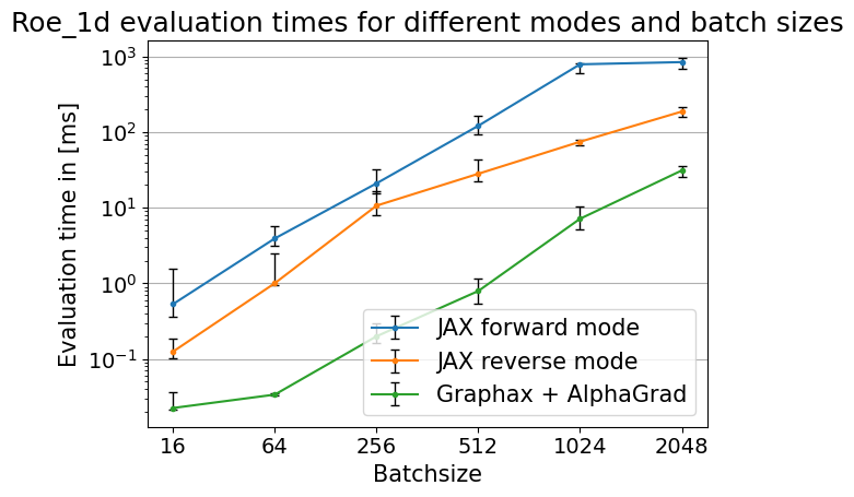
(a) RoeFlux_1d

(b) RobotArm_6DOF

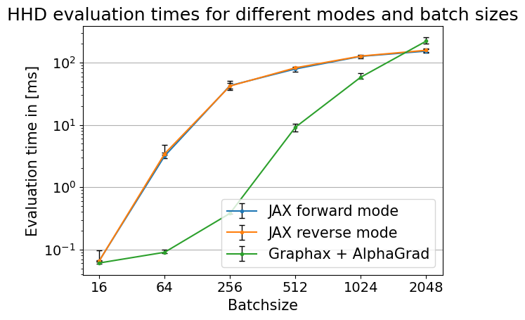
(c) HumanHeartDipole

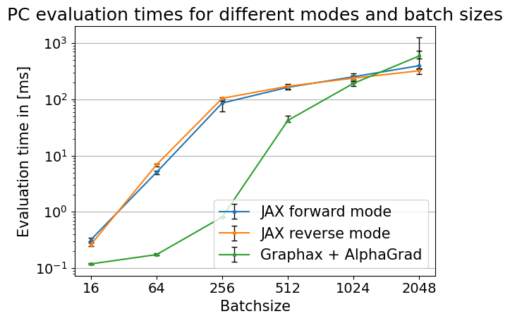
(d) PropaneCombustion

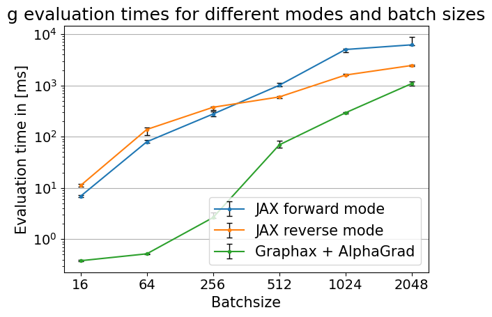
(e) Random function $g$

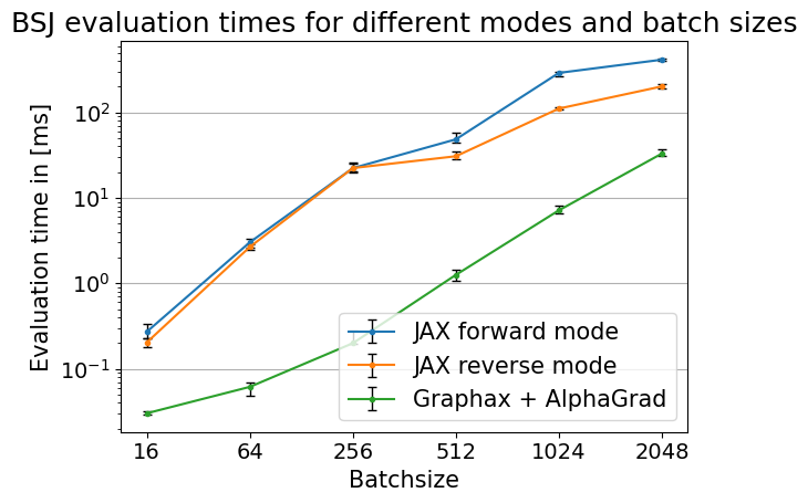
(f) BlackScholes_Jacobian

Figure 4: Runtime measurements over 100 trials for the scalar tasks. Error bars are the 2.5- and 97.5-percentiles of the runtimes.

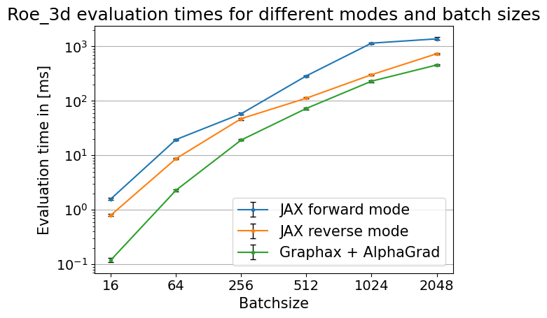
(a) RoeFlux_3d

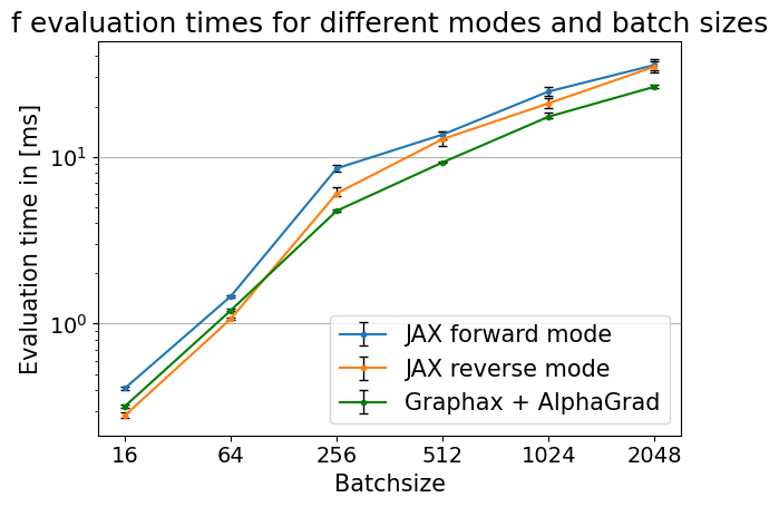
(b) Random function $f$

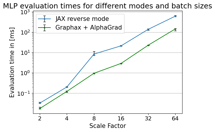
(c) Multi-Layer Perceptron

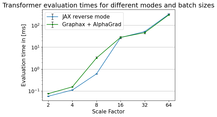
(d) Transformer Encoder

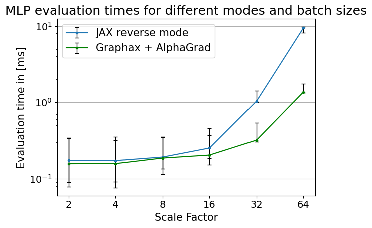
(e) Multi-Layer Perceptron (GPU)

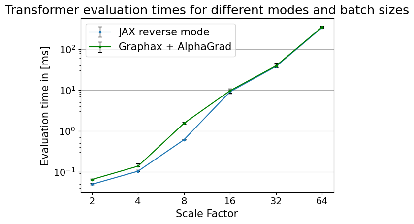
(f) Transformer Encoder (GPU)

Figure 5: Runtime measurements over 100 trials for the vectorized tasks with different batchsizes. The MLP network sizes were scaled up with growing batchsize. The transformer could only be evaluated on with a batchsize of 1 due to limitations of VertexGame but the network size was scaled up as well. Both deep learning tasks were also evaluated on GPUs. Error bars are the 2.5- and 97.5-percentiles of the runtimes.

Appendix C Sparsity Types

The sparsity of the Jacobians associated with the edges in the computational graph representation is described with a number ranging from -10 to 10. Table 3 contains an overview of the sparsity types and an example tensor that is represented by the corresponding number. Our approach is directed only at diagonal sparsity, meaning that we mainly consider tensors that can be decomposed into products of lower-dimensional tensors and Kronecker symbols $\delta_{ij}$. Since we might have operations like transposing or slicing in our computational graph, which just change the shape but not the value of the edge Jacobians when eliminated, we introduce a “copy gradient” sparsity type with value -1 to represent these operations. Furthermore, we make a distinction between multiplication with the unit tensor $c\delta_{il}\delta_{jk}$ and a constant multiple of the unit tensor $c\delta_{il}\delta_{jk}$ since the latter incurs actual multiplications while the former can just be treated as a renaming of indices as demonstrated by the following examples with tensors $S_{klmn}=\delta_{km}\delta_{ln}$ and $U_{klmn}=c\delta_{km}\delta_{ln}$ :

$$\sum_{kl}T_{ij}\delta_{ik}\delta_{jl}\cdot\delta_{km}\delta_{ln} =T_{ij}\delta_{im}\delta_{jn},$$ (7)

$$\sum_{kl}T_{ij}\delta_{ik}\delta_{jl}\cdot c\delta_{km}\delta_{ln} =cT_{ij}\delta_{im}\delta_{jn}.$$ (8)

In the first equation, we can just rename the indices of the tensor, but in the second equation we have to perform the product $cT_{ij}$, which incurs $|i|\cdot|j|$ multiplications. If two edges are multiplied with each other, we determine the resulting sparsity type of the new edge by looking up the combination in a large handcrafted table and then writing the result into the new graph representation. The new shape of the Jacobian is determined according to the rules of tensor contraction. Finally we delete the old edges from the representation as required by the vertex elimination procedure. The sparse matrix multiplication table for the computational graph representation can be found in the accompanying source code. The number of multiplications incurred by a multiplication of two edge Jacobians is computed from the sparsity types involved and the Jacobian shapes. By multiplying all values of the two Jacobian shapes with each other and masking out certain values according to the sparsity types involved, we arrive at the correct number of multiplications. For examples consider two tensors $S_{ijkl}=a_{ij}\delta_{ik}\delta_{jl}$ with sizes $(2,3,2,3)$ with sparsity type 6 and $T_{ijkl}=b_{i}\delta_{il}\delta_{jk}$ with shape $(2,3,2,3)$ and sparsity type 9. Thus, in the computational graph representation, we would have two non-zero entries $(6,2,3,2,3)$ and $(9,2,3,2,3)$. Then their contraction is given through

$$\sum_{kl}S_{ijkl}T_{klmn}=\sum_{kl}a_{ij}\delta_{ik}\delta_{jl}\cdot b_{k}\delta_{kn}\delta_{lm}=a_{ij}b_{n}\delta_{in}\delta_{jm}.$$ (9)

Then we form the product $|i|\cdot|j|\cdot|k|\cdot|l|\cdot|m|\cdot|n|=2\cdot 3\cdot 2\cdot 3\cdot 2\cdot 3$ where $|\cdot|$ gives the size of the dimension associated with the index. Then we use the sparsity types 7 and 9 to mask out the relevant values. In this case, we mask out $|k|$, $|l|$ and $|m|$ such that we arrive at $|i|\cdot|j|\cdot|n|=2\cdot 3\cdot 3=18$ multiplications which is exactly the number of multiplications incurred by the dense multiplication of $a_{ij}b_{n}$.

Table 3: Different sparsity types that are required to represent all the possible tensor shapes that occur in tensor vertex elimination with vectors and matrices.

Sparsity Type	Example Tensor
-10	$c\delta_{il}\delta_{jk}$
-9	$T_{j}\delta_{il}\delta_{jk}$
-8	$T_{j}\delta_{ik}\delta_{jl}$
-7	$\delta_{il}\delta_{jk}$
-6	$\delta_{ik}\delta_{jl}$
-5	$T_{il}\delta_{jk}$
-4	$T_{jk}\delta_{il}$
-3	$T_{ik}\delta_{jl}$
-2	$T_{jl}\delta_{ik}$
-1	copy gradient operation
0	no edge
1	$T_{ijkl}$
2	$T_{ijl}\delta_{ik}$
3	$T_{ijk}\delta_{jl}$
4	$T_{jk}\delta_{il}$
5	$T_{il}\delta_{jk}$
6	$T_{ij}\delta_{ik}\delta_{jl}$
7	$T_{ij}\delta_{il}\delta_{jk}$
8	$T_{i}\delta_{ik}\delta_{jl}$
9	$T_{i}\delta_{il}\delta_{jk}$
10	$c\delta_{ik}\delta_{jl}$

Appendix D RL Algorithm and Network Architecture

We solved VertexGame with PPO [Schulman et al., 2017] and AlphaZero [Schrittwieser et al., 2019] and used a similar architecture backbone in both cases:

• Convolutional embedding to compress the computational graph representation down using a 3x5 kernel mapped across the sequence dimension, i.e. the 3x5 filter was applied to all tokens to reduce the feature dimension. Since the computational graph representation is very sparse as each vertex typically only has a few connections to other vertices.

• Linear projection to an embedding size of 64.

• Positional encoding as described in [Vaswani et al., 2017].

• Multiple transformer layers with embedding size 64, softmax-attention, layer norm and two MLP layers with a hidden layer size of 256.

In the PPO case, we used two such backbones of with 5 and 4 transformer layers for separate policy and value networks. The policy head was an MLP of with hidden layers of sizes (256, 128) and output size 1 while the value head used an MLP with hidden layers of sizes (256, 128, 64) again with output size 1. The AlphaZero agent used the same heads on a single transformer backbone with 6 transformer layers. In all cases, the MLPs are mapped over the sequence dimension. For the policy head, this produces an unnormalized probability distribution over the actions while for the value head, we first sum all outputs to get an estimate of the input state value.

PPO Implementation Details

We tightly followed [Huang et al., 2022] for the implementation of the PPO agent. Unless otherwise specified, all models were trained on 32 parallel environments with 4 minibatches and a clipping parameter of 0.2. We set the value and entropy weights to 1.0 and 0.01 respectively, while the learning rate was fixed to $2.5\cdot 10^{-4}$. However, we found that the agent performed best if the rollout length was set to be equal to the number of intermediate vertices, although this is technically an implementation error.

AlphaZero Implementation Details

The implementation is loosely based on the implementation of Gumbel MuZero and uses the mctx package provided by Google DeepMind [DeepMind et al., 2020]. However, we modified the implementation by replacing the trainable model and reward functions with our deterministic implementation of the VertexGame environment, thus effectively creating a Gumbel AlphaZero agent. Unless otherwise specified, all models were trained on 32 parallel environments with batchsize 4096 and 50 MCTS simulations with 5 considered actions. We set the value and L2 weights to 10.0 and 0.01 respectively, while the learning rate was set to $1\cdot 10^{-3}$ with a cosine learning rate annealing over 5000 episodes. For Gumbel MuZero to work properly, it is necessary to rescale the rewards so that they lie in the interval [0,1). In the Gumbel MuZero paper, the authors designed a specific transformation that normalizes the rewards and simultaneously completes the missing values using the Gumbel distribution. The parameters of this transformation have to be carefully tuned to enable learning. In our case, we set the corresponding parameters to $c_{\mathrm{visit}}=25$ and $c_{\mathrm{scale}}=0.01$ for all cases. We trained the agent using adaptive momentum gradient-based learning [Kingma and Ba, 2014] with an initial learning rate of $10^{-3}$ and cosine learning rate scheduling over 5000 episodes on two to four NVIDIA RTX 4090 GPUs.

Appendix E AlphaZero Results

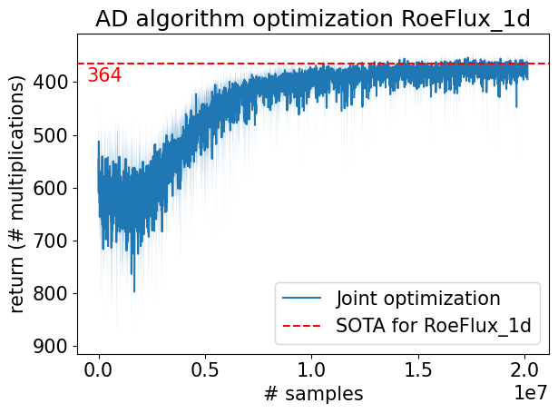
(a) RoeFlux_1d

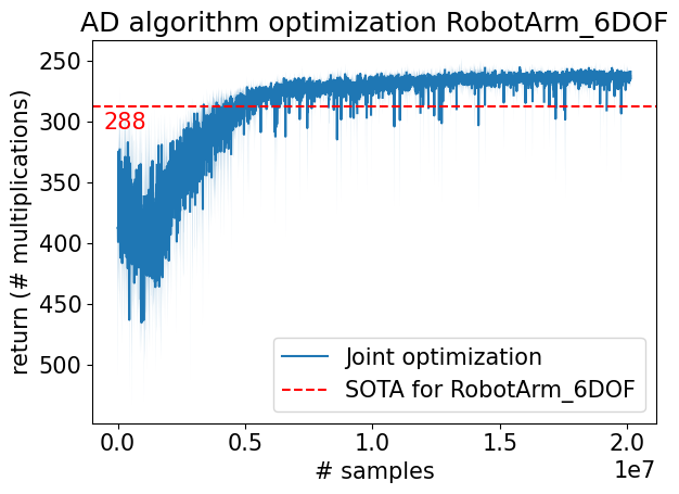
(b) RobotArm_6DOF

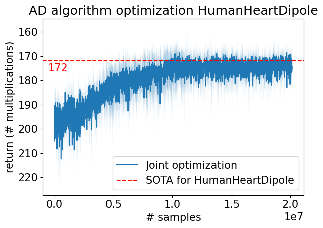
(c) HumanHeartDipole

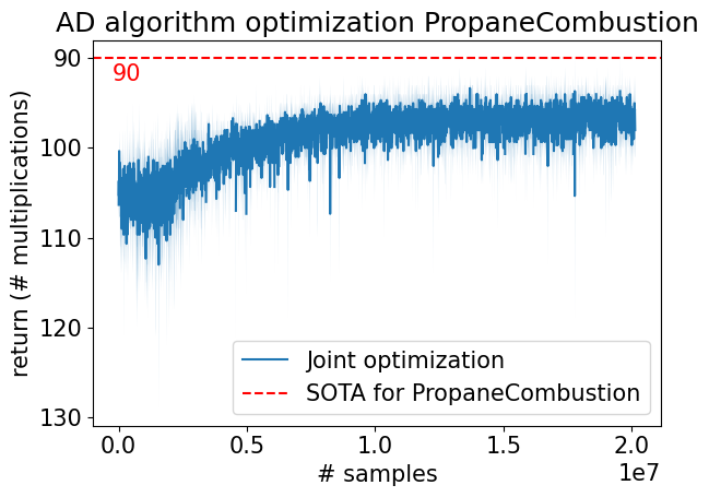
(d) PropaneCombustion

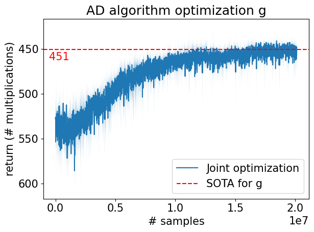
(e) Random function $g$

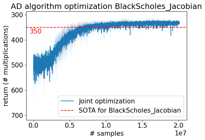
(f) BlackScholes_Jacobian

Figure 8: Learning curves of the scalar tasks in joint training mode for the same three random seeds with the AlphaZero-based agent. The best result for each task is displayed in table 6.

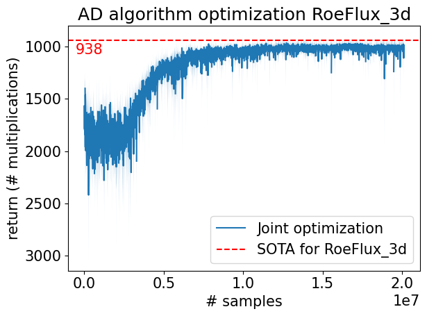
(a) RoeFlux_3d

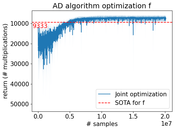
(b) Random function $f$

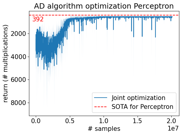
(c) Multi-Layer Perceptron

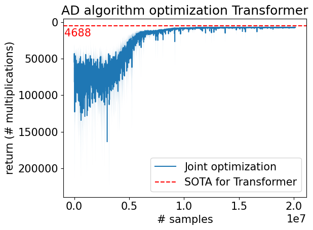
(d) Transformer Encoder

Figure 9: Learning curves of the vectorized tasks in joint training mode for the same three random seeds for the AlphaZero-based agent. The best result for each task is displayed in table 6.

This section contains the reward curves and elimination orders for the results presented in tables 1 and 2. Reward curves are shown for six different random seeds, namely 42, 123, 541, 1337, 1743 and 250197. The elimination orders can be directly used with the accompanying Graphax package using the graphax.jacve command that creates the Jacobian for a given function $f$ and a given order through graphax.jacve(f, order=order, argnums=argnums)(*xs). The orders given in tables 4 and 5 can be directly used to compute the Jacobians.
In addition to the single-graph experiments where the agent was trained only on a single task, we also experimented with training the agent on all tasks at once. For this, we randomly sampled from the 10 defined tasks to create 32 random environments. The agent was trained with the same configuration as for the single task experiments. The results are shown in figures 8 and 9 and the best achieved numbers of multiplication are displayed in table 6.

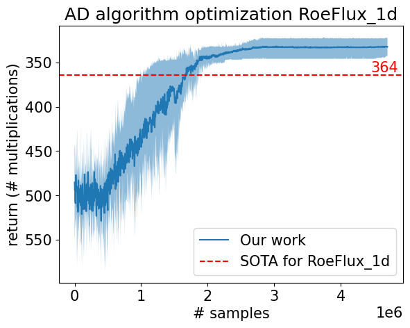
(a) RoeFlux_1d

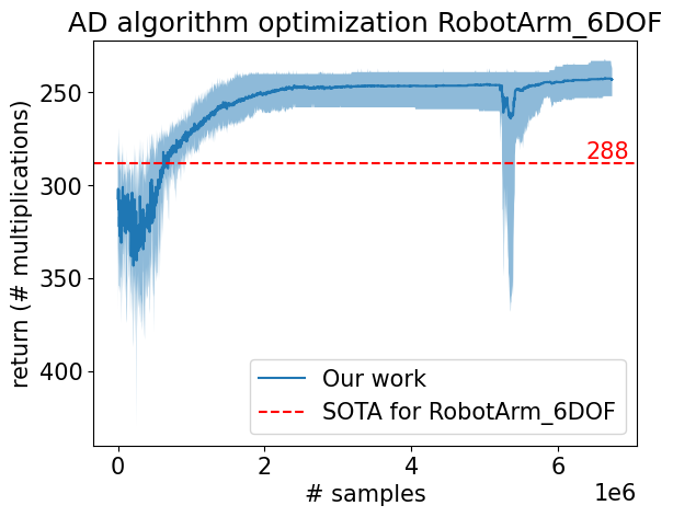
(b) RobotArm_6DOF

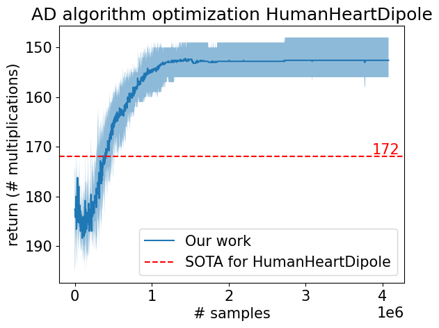
(c) HumanHeartDipole

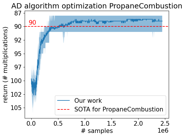
(d) PropaneCombustion

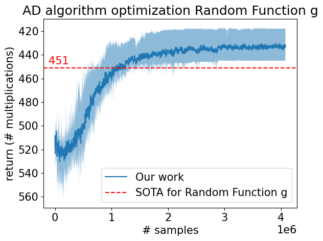
(e) Random function $g$

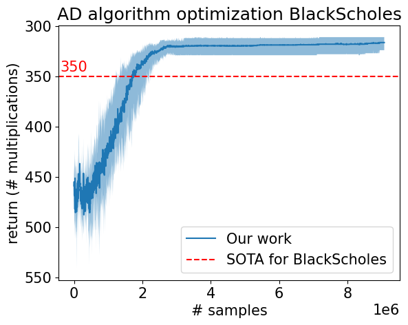
(f) BlackScholes_Jacobian

Figure 6: Learning curves of the scalar tasks for the same six random seeds with the AlphaZero-based agent. AlphaGrad manages to find better elimination orders for all tasks. The best result for each task is displayed in table 1.

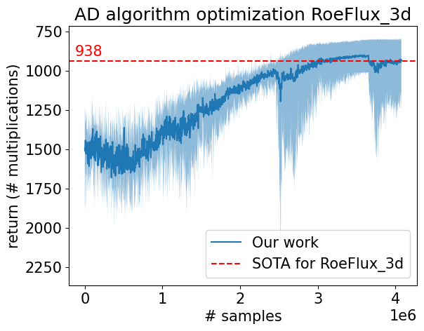
(a) RoeFlux_3d

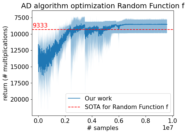
(b) Random function $f$

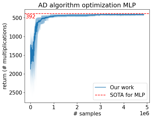
(c) Multi-Layer Perceptron

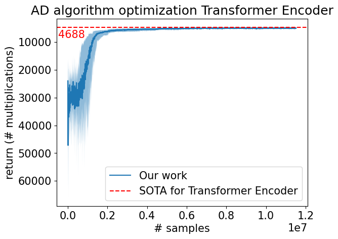
(d) Transformer Encoder

Figure 7: Learning curves of the vectorized tasks for the same six random seeds for the AlphaZero-based agent. AlphaGrad manages to find better elimination orders for all tasks. The best result for each task is displayed in table 1.

Table 4: Elimination orders for the results obtained with AlphaGrad presented in table 1.

Task	# multiplications	Elimination Order
RoeFlux_1d	320	[8, 82, 27, 66, 7, 78, 76, 13, 48, 42, 68, 86, 95, 4, 59,
		28, 77, 54, 1, 94, 5, 58, 72, 93, 75, 31, 53, 33, 57, 90,
		44, 25, 89, 88, 84, 96, 74, 92, 83, 91, 45, 51, 81, 80, 11,
		10, 85, 43, 22, 73, 19, 71, 6, 18, 17, 79, 47, 50, 52, 21,
		37, 38, 55, 49, 69, 35, 65, 29, 64, 16, 9, 60, 15, 61, 23,
		87, 70, 67, 24, 46, 63, 39, 2, 62, 3, 41, 40, 32, 26, 34, 56,
		30, 14, 98, 36, 12, 20, 100]
RobotArm_6DOF	231	[37, 18, 22, 41, 40, 8, 9, 101, 64, 36, 32, 61, 21, 14, 63,
		2, 23, 82, 67, 7, 94, 15, 52, 49, 20, 97, 74, 93, 34, 77, 6,
		31, 30, 104, 51, 103, 33, 105, 65, 76, 48, 45, 90, 44, 99,
		95, 47, 46, 55, 73, 84, 29, 19, 79, 26, 57, 42, 43, 16, 92,
		113, 112, 110, 53, 89, 35, 88, 107, 72, 70, 50, 71, 39, 83,
		78, 111, 60, 58, 81, 38, 28, 5, 87, 108, 3, 91, 86, 109, 27,
		54, 69, 25, 17, 106, 56, 10, 11, 75, 100, 1, 59, 98, 80, 4,
		96, 13, 24, 12]
HumanHeartDipole	148	[19, 85, 11, 83, 77, 59, 81, 22, 76, 1, 9, 37, 49, 68, 69, 7,
		3, 45, 51, 17, 75, 34, 66, 36, 61, 73, 71, 48, 79, 57, 40, 8,
		24, 43, 39, 21, 52, 53, 16, 56, 67, 28, 42, 54, 33, 31, 30,
		74, 10, 27, 47, 63, 44, 46, 6, 72, 32, 58, 55, 15, 41, 29, 13,
		82, 80, 25, 26, 18, 14, 62, 5, 60, 84, 35, 64, 23, 65, 70]
PropaneCombustion	88	[12, 51, 33, 45, 10, 9, 42, 39, 1, 18, 27, 8, 61, 60, 48, 59,
		36, 35, 34, 24, 26, 30, 23, 44, 43, 58, 50, 32, 40, 57, 56,
		55, 54, 28, 38, 20, 21, 3, 15, 7, 2, 29, 17, 53, 5, 47, 6, 16,
		14, 11, 49]
Random function $g$	417	[1, 99, 85, 90, 87, 47, 51, 20, 3, 66, 49, 64, 13, 11, 22,
		39, 61, 43, 31, 2, 6, 92, 89, 29, 16, 82, 86, 60, 24, 19, 79,
		56, 63, 15, 73, 57, 50, 33, 4, 36, 70, 41, 67, 54, 30, 14,
		8, 53, 78, 46, 42, 18, 17, 62, 68, 76, 65, 23, 7, 58, 38, 52,
		26, 91, 34, 45, 21, 40, 35, 12, 44, 75, 25, 5, 48, 10, 59,
		84, 27, 9, 71, 37, 32, 28, 74]
BlackScholes	312	[70, 16, 104, 43, 11, 15, 36, 71, 62, 42, 57, 24, 101, 74,
		54, 96, 64, 65, 119, 14, 118, 50, 76, 61, 32, 19, 17, 45,
		40, 59, 100, 68, 49, 126, 114, 83, 60, 116, 113, 20, 78,
		25, 121, 6, 48, 31, 84, 66, 18, 28, 133, 10, 12, 58, 13,
		87, 110, 29, 46, 38, 120, 92, 21, 77, 44, 107, 105, 81,
		7, 56, 47, 55, 124, 67, 75, 93, 95, 79, 89, 86, 103, 82, 37,
		94, 8, 52, 1, 111, 106, 23, 9, 53, 85, 90, 112, 69, 41, 34,
		98, 35, 51, 22, 80, 72, 115, 91, 33, 39, 27, 99, 30, 88,
		131, 123, 117, 73, 2, 109, 26, 5, 63, 128, 108, 4, 97, 102,
		3, 125, 130]

Table 5: Elimination orders for the results obtained with AlphaGrad presented in table 1 (ctd.).

Task	# multiplications	Elimination Order
RoeFlux_3d	811	[124, 136, 56, 128, 78, 24, 1, 54, 101, 127, 121, 140,
		47, 135, 67, 34, 111, 32, 100, 119, 99, 114, 125, 141,
		122, 45, 65, 59, 117, 89, 116, 60, 42, 28, 74, 85, 11, 53,
		36, 30, 108, 113, 55, 109, 129, 64, 91, 14, 133, 5, 10,
		132, 87, 139, 110, 12, 131, 72, 8, 61, 88, 107, 6, 29,
		57, 96, 118, 105, 71, 77, 112, 66, 75, 84, 143, 123, 90,
		94, 137, 104, 69, 23, 22, 62, 58, 50, 130, 31, 106, 39,
		48, 49, 98, 134, 93, 138, 126, 68, 115, 80, 102, 92, 79,
		52, 16, 120, 95, 76, 19, 25, 73, 21, 70, 38, 35, 20, 86,
		41, 4, 103, 43, 27, 3, 40, 9, 83, 13, 18, 37, 51, 46, 7,
		81, 97, 63, 44, 2, 33, 82, 26, 15, 17, 145]
Random function $f$	6374	[33, 8, 16, 77, 15, 62, 40, 58, 14, 76, 42, 60, 54, 34, 61, 72,
		37, 55, 18, 75, 36, 74, 65, 26, 35, 25, 66, 38, 64, 59, 53, 20,
		27, 47, 10, 69, 23, 11, 41, 79, 9, 7, 12, 63, 71, 24, 67, 51, 4,
		1, 21, 3, 6, 2, 49, 13, 44, 46, 56, 17, 39, 57, 43, 32, 52, 30,
		48, 31, 5, 22, 45, 19, 50, 28, 29]
2-layer MLP†	389	[21, 29, 17, 15, 3, 28, 25, 30, 19, 34, 13, 8, 12, 36, 38,
		31, 37, 35, 27, 33, 10, 32, 26, 20, 24, 23, 22, 18, 16,
		14, 11, 9, 7, 6, 5, 4, 2, 1]
Encoder†	4656	[60, 81, 8, 59, 58, 41, 69, 85, 1, 46, 25, 51, 37, 17, 56, 22,
		12, 75, 78, 82, 7, 66, 47, 64, 20, 88, 65, 31, 38, 6, 63, 71,
		87, 19, 90, 24, 80, 83, 27, 48, 77, 49, 29, 23, 76, 9, 79, 67,
		61, 26, 89, 86, 18, 34, 39, 84, 74, 70, 30, 36, 35, 72, 50,
		73, 68, 62, 57, 28, 5, 55, 13, 11, 54, 53, 43, 52, 45, 44, 42,
		40, 33, 32, 21, 16, 15, 14, 3, 10, 4, 2]

Table 6: Best number of multiplications achieved in joint training mode with the AlphaZero-based agent.

RoeFlux_1d	RobotArm_6DOF	HumanHeartDipole	PropaneCombustion	$g$
331	248	158	n.a.	430
RoeFlux_3d	MLP	Encoder	BlackScholes_Jacobian	$f$
907	n.a.	n.a.	307	5884

Appendix F PPO Results

We ran all experiments with the configuration described in D and used the random seeds from the AlphaZero experiments. The PPO agent also manages to find better elimination orders that improve over the state-of-the-art but is outperformed by the AlphaZero agent on all tasks, sometimes by a significant margin as for example in the RoeFlux tasks and random function $f$ or the MLP and TransformerEncoder where it does not find a better elimination order at all. This is to be expected since the AlphaZero agent can make use of the available model and thus select actions through planning. In other cases, the performance comes very close to the AlphaZero agent, for example in the BlackScholes_Jacobian or random function $f$ tasks. Thus, the PPO-based agent might still be a viable choice because it is trained within minutes on a single NVIDIA RTX 4090 GPU, even for large tasks such as the random function $f$ and still find well-performing elimination orders. Table 7 shows the number of multiplications required by the best elimination order found by the PPO-agent. Figures 10 and 11 contain the corresponding reward curves. We did not succeed in training a joint model using the PPO agent.

Table 7: Best number of multiplications achieved by the PPO-based agent.

RoeFlux_1d	RobotArm_6DOF	HumanHeartDipole	PropaneCombustion	$g$
324	245	162	n.a.	422
RoeFlux_3d	MLP	Encoder	BlackScholes_Jacobian	$f$
885	n.a.	n.a.	313	6497

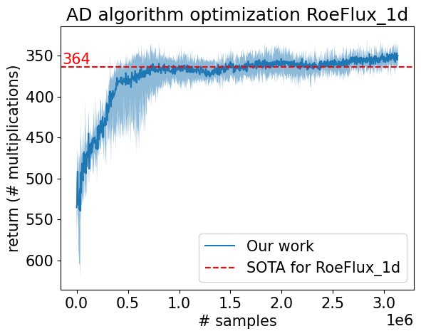
(a) RoeFlux_1d

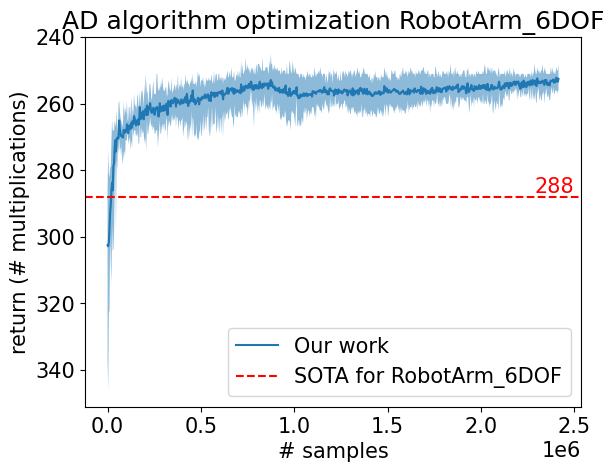
(b) RobotArm_6DOF

(c) HumanHeartDipole

(d) PropaneCombustion

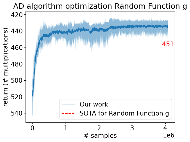
(e) Random function $g$

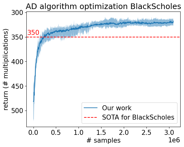
(f) BlackScholes_Jacobian

Figure 10: Learning curves of the scalar tasks for the same six random seeds with the PPO-based agent. It manages to find better elimination orders for many of the tasks. The best result for each task is displayed in table 7.

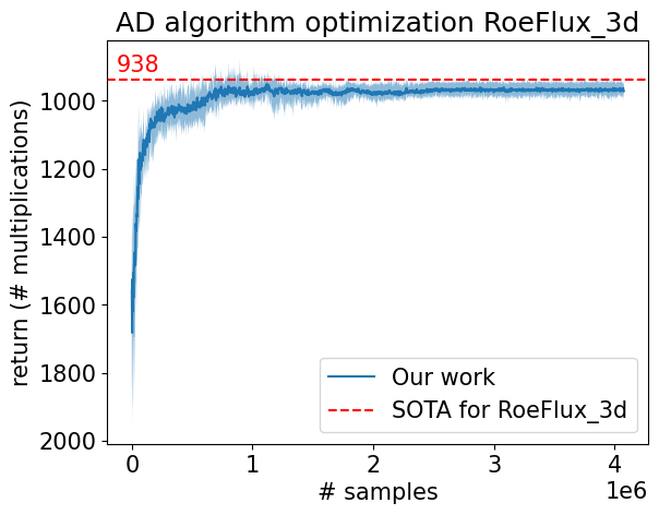
(a) RoeFlux_3d

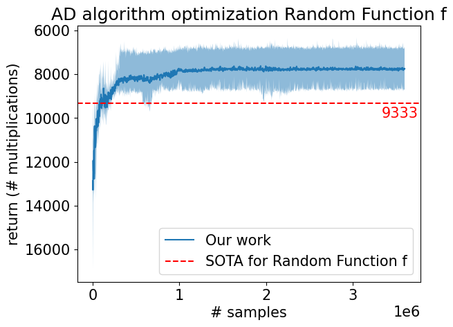
(b) Random function $f$

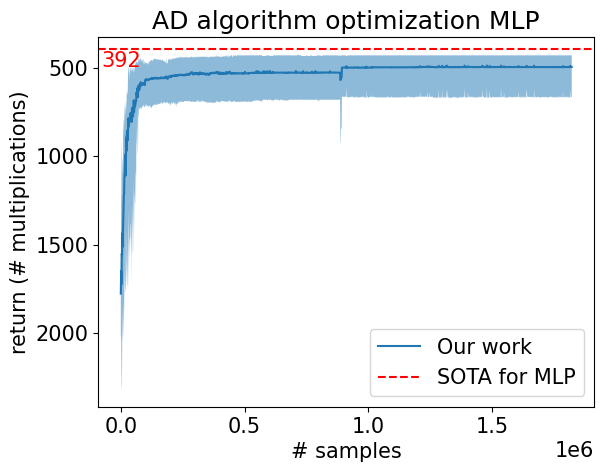
(c) Multi-Layer Perceptron

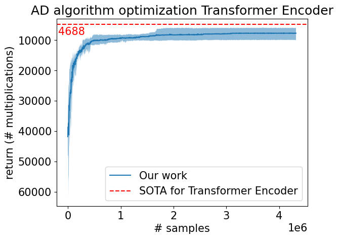
(d) Transformer Encoder

Figure 11: Learning curves of the vectorized tasks for the same six random seeds for the PPO-based agent. It manages to find better elimination orders for all tasks. The best result for each task is displayed in table 7.

NeurIPS Paper Checklist

1. Claims

2. Question: Do the main claims made in the abstract and introduction accurately reflect the paper’s contributions and scope?

3. Answer: [Yes]

4. Justification: The claims contained in the abstract reflect exactly the content of the work. In the abstract, we make statements about theoretical and practical improvements in automatic differentiation. In the experiments section we provide empirical proof for both.

5. Guidelines:

   • The answer NA means that the abstract and introduction do not include the claims made in the paper.

   • The abstract and/or introduction should clearly state the claims made, including the contributions made in the paper and important assumptions and limitations. A No or NA answer to this question will not be perceived well by the reviewers.

   • The claims made should match theoretical and experimental results, and reflect how much the results can be expected to generalize to other settings.

   • It is fine to include aspirational goals as motivation as long as it is clear that these goals are not attained by the paper.

6. Limitations

7. Question: Does the paper discuss the limitations of the work performed by the authors?

8. Answer: [Yes]

9. Justification: The paper clearly describes the limitations of the approach by including negative outcomes in the the experimental results table and provides a more in-depth analysis in the discussion and appendix sections of the paper.

10. Guidelines:

    • The answer NA means that the paper has no limitation while the answer No means that the paper has limitations, but those are not discussed in the paper.

    • The authors are encouraged to create a separate "Limitations" section in their paper.

    • The paper should point out any strong assumptions and how robust the results are to violations of these assumptions (e.g., independence assumptions, noiseless settings, model well-specification, asymptotic approximations only holding locally). The authors should reflect on how these assumptions might be violated in practice and what the implications would be.

    • The authors should reflect on the scope of the claims made, e.g., if the approach was only tested on a few datasets or with a few runs. In general, empirical results often depend on implicit assumptions, which should be articulated.

    • The authors should reflect on the factors that influence the performance of the approach. For example, a facial recognition algorithm may perform poorly when image resolution is low or images are taken in low lighting. Or a speech-to-text system might not be used reliably to provide closed captions for online lectures because it fails to handle technical jargon.

    • The authors should discuss the computational efficiency of the proposed algorithms and how they scale with dataset size.

    • If applicable, the authors should discuss possible limitations of their approach to address problems of privacy and fairness.

    • While the authors might fear that complete honesty about limitations might be used by reviewers as grounds for rejection, a worse outcome might be that reviewers discover limitations that aren’t acknowledged in the paper. The authors should use their best judgment and recognize that individual actions in favor of transparency play an important role in developing norms that preserve the integrity of the community. Reviewers will be specifically instructed to not penalize honesty concerning limitations.

11. Theory Assumptions and Proofs

12. Question: For each theoretical result, does the paper provide the full set of assumptions and a complete (and correct) proof?

13. Answer: [N/A]

14. Justification:

15. Guidelines:

    • The answer NA means that the paper does not include theoretical results.

    • All the theorems, formulas, and proofs in the paper should be numbered and cross-referenced.

    • All assumptions should be clearly stated or referenced in the statement of any theorems.

    • The proofs can either appear in the main paper or the supplemental material, but if they appear in the supplemental material, the authors are encouraged to provide a short proof sketch to provide intuition.

    • Inversely, any informal proof provided in the core of the paper should be complemented by formal proofs provided in appendix or supplemental material.

    • Theorems and Lemmas that the proof relies upon should be properly referenced.

16. Experimental Result Reproducibility

17. Question: Does the paper fully disclose all the information needed to reproduce the main experimental results of the paper to the extent that it affects the main claims and/or conclusions of the paper (regardless of whether the code and data are provided or not)?

18. Answer: [Yes]

19. Justification: The entire codebase as well as a comprehensive tutorial will be provided with the paper as part of a GitHub repository. Furthermore, the appendix includes implementation details on the RL algorithms and neural networks as well as an in-depth description of the functions that were analyzed and all the best performing elimination orders. Furthermore, the reviewers will be provided with full access to the entire codebase on submission.

20. Guidelines:

    • The answer NA means that the paper does not include experiments.

    • If the paper includes experiments, a No answer to this question will not be perceived well by the reviewers: Making the paper reproducible is important, regardless of whether the code and data are provided or not.

    • If the contribution is a dataset and/or model, the authors should describe the steps taken to make their results reproducible or verifiable.

    • Depending on the contribution, reproducibility can be accomplished in various ways. For example, if the contribution is a novel architecture, describing the architecture fully might suffice, or if the contribution is a specific model and empirical evaluation, it may be necessary to either make it possible for others to replicate the model with the same dataset, or provide access to the model. In general. releasing code and data is often one good way to accomplish this, but reproducibility can also be provided via detailed instructions for how to replicate the results, access to a hosted model (e.g., in the case of a large language model), releasing of a model checkpoint, or other means that are appropriate to the research performed.

    • While NeurIPS does not require releasing code, the conference does require all submissions to provide some reasonable avenue for reproducibility, which may depend on the nature of the contribution. For example

      1. If the contribution is primarily a new algorithm, the paper should make it clear how to reproduce that algorithm.

      2. If the contribution is primarily a new model architecture, the paper should describe the architecture clearly and fully.

      3. If the contribution is a new model (e.g., a large language model), then there should either be a way to access this model for reproducing the results or a way to reproduce the model (e.g., with an open-source dataset or instructions for how to construct the dataset).

      4. We recognize that reproducibility may be tricky in some cases, in which case authors are welcome to describe the particular way they provide for reproducibility. In the case of closed-source models, it may be that access to the model is limited in some way (e.g., to registered users), but it should be possible for other researchers to have some path to reproducing or verifying the results.

21. Open access to data and code

22. Question: Does the paper provide open access to the data and code, with sufficient instructions to faithfully reproduce the main experimental results, as described in supplemental material?

23. Answer: [Yes]

24. Justification: The entire codebase along with a comprehensive introduction will be published on release of the work. Furthermore, the reviewers will be provided with full access to the entire codebase on submission. Also, all novel elimination orders are provided in the appendix.

25. Guidelines:

    • The answer NA means that paper does not include experiments requiring code.

    • Please see the NeurIPS code and data submission guidelines (https://nips.cc/public/guides/CodeSubmissionPolicy) for more details.

    • While we encourage the release of code and data, we understand that this might not be possible, so “No” is an acceptable answer. Papers cannot be rejected simply for not including code, unless this is central to the contribution (e.g., for a new open-source benchmark).

    • The instructions should contain the exact command and environment needed to run to reproduce the results. See the NeurIPS code and data submission guidelines (https://nips.cc/public/guides/CodeSubmissionPolicy) for more details.

    • The authors should provide instructions on data access and preparation, including how to access the raw data, preprocessed data, intermediate data, and generated data, etc.

    • The authors should provide scripts to reproduce all experimental results for the new proposed method and baselines. If only a subset of experiments are reproducible, they should state which ones are omitted from the script and why.

    • At submission time, to preserve anonymity, the authors should release anonymized versions (if applicable).

    • Providing as much information as possible in supplemental material (appended to the paper) is recommended, but including URLs to data and code is permitted.

26. Experimental Setting/Details

27. Question: Does the paper specify all the training and test details (e.g., data splits, hyperparameters, how they were chosen, type of optimizer, etc.) necessary to understand the results?

28. Answer: [Yes]

29. Justification: All necessary experimental parameters like learning rates, RL configuration etc. are provided in the appendix and as .yaml files in the source code of the model.

30. Guidelines:

    • The answer NA means that the paper does not include experiments.

    • The experimental setting should be presented in the core of the paper to a level of detail that is necessary to appreciate the results and make sense of them.

    • The full details can be provided either with the code, in appendix, or as supplemental material.

31. Experiment Statistical Significance

32. Question: Does the paper report error bars suitably and correctly defined or other appropriate information about the statistical significance of the experiments?

33. Answer: [Yes]

34. Justification: The key results of the paper are runtime measurements that do not necessarily follow a Gaussian normal distribution. The authors therefore decided to display results using the median and 2.5- and 97.5-percentiles to quantify the uncertainty.

35. Guidelines:

    • The answer NA means that the paper does not include experiments.

    • The authors should answer "Yes" if the results are accompanied by error bars, confidence intervals, or statistical significance tests, at least for the experiments that support the main claims of the paper.

    • The factors of variability that the error bars are capturing should be clearly stated (for example, train/test split, initialization, random drawing of some parameter, or overall run with given experimental conditions).

    • The method for calculating the error bars should be explained (closed form formula, call to a library function, bootstrap, etc.)

    • The assumptions made should be given (e.g., Normally distributed errors).

    • It should be clear whether the error bar is the standard deviation or the standard error of the mean.

    • It is OK to report 1-sigma error bars, but one should state it. The authors should preferably report a 2-sigma error bar than state that they have a 96% CI, if the hypothesis of Normality of errors is not verified.

    • For asymmetric distributions, the authors should be careful not to show in tables or figures symmetric error bars that would yield results that are out of range (e.g. negative error rates).

    • If error bars are reported in tables or plots, The authors should explain in the text how they were calculated and reference the corresponding figures or tables in the text.

36. Experiments Compute Resources

37. Question: For each experiment, does the paper provide sufficient information on the computer resources (type of compute workers, memory, time of execution) needed to reproduce the experiments?

38. Answer: [Yes]

39. Justification: Details about the hardware requirements are included in the appendix of the paper.

40. Guidelines:

    • The answer NA means that the paper does not include experiments.

    • The paper should indicate the type of compute workers CPU or GPU, internal cluster, or cloud provider, including relevant memory and storage.

    • The paper should provide the amount of compute required for each of the individual experimental runs as well as estimate the total compute.

    • The paper should disclose whether the full research project required more compute than the experiments reported in the paper (e.g., preliminary or failed experiments that didn’t make it into the paper).

41. Code Of Ethics

42. Question: Does the research conducted in the paper conform, in every respect, with the NeurIPS Code of Ethics https://neurips.cc/public/EthicsGuidelines?

43. Answer: [Yes] .

44. Justification: The authors have read the NeurIPS ethics code and are sure that the research conducted in this paper as well as the results of the paper did not violate any of the points raised in the guidelines. The main result of the paper is a way to find faster and more energy-efficient automatic differentiation algorithms which to the authors best knowledge does not pose any harm to humanity and nature. Furthermore, all libraries used in this work are publicly available under very lenient licensing.

45. Guidelines:

    • The answer NA means that the authors have not reviewed the NeurIPS Code of Ethics.

    • If the authors answer No, they should explain the special circumstances that require a deviation from the Code of Ethics.

    • The authors should make sure to preserve anonymity (e.g., if there is a special consideration due to laws or regulations in their jurisdiction).

46. Broader Impacts

47. Question: Does the paper discuss both potential positive societal impacts and negative societal impacts of the work performed?

48. Answer: [Yes]

49. Justification: The main result of the paper is a way to find faster and more energy-efficient automatic differentiation algorithms which most likely has a positive impact on the environment as it might reduce the energy consumption of many computational workloads. The authors are not aware of any possible negative influences.

50. Guidelines:

    • The answer NA means that there is no societal impact of the work performed.

    • If the authors answer NA or No, they should explain why their work has no societal impact or why the paper does not address societal impact.

    • Examples of negative societal impacts include potential malicious or unintended uses (e.g., disinformation, generating fake profiles, surveillance), fairness considerations (e.g., deployment of technologies that could make decisions that unfairly impact specific groups), privacy considerations, and security considerations.

    • The conference expects that many papers will be foundational research and not tied to particular applications, let alone deployments. However, if there is a direct path to any negative applications, the authors should point it out. For example, it is legitimate to point out that an improvement in the quality of generative models could be used to generate deepfakes for disinformation. On the other hand, it is not needed to point out that a generic algorithm for optimizing neural networks could enable people to train models that generate Deepfakes faster.

    • The authors should consider possible harms that could arise when the technology is being used as intended and functioning correctly, harms that could arise when the technology is being used as intended but gives incorrect results, and harms following from (intentional or unintentional) misuse of the technology.

    • If there are negative societal impacts, the authors could also discuss possible mitigation strategies (e.g., gated release of models, providing defenses in addition to attacks, mechanisms for monitoring misuse, mechanisms to monitor how a system learns from feedback over time, improving the efficiency and accessibility of ML).

51. Safeguards

52. Question: Does the paper describe safeguards that have been put in place for responsible release of data or models that have a high risk for misuse (e.g., pretrained language models, image generators, or scraped datasets)?

53. Answer: [N/A] .

54. Justification:

55. Guidelines:

    • The answer NA means that the paper poses no such risks.

    • Released models that have a high risk for misuse or dual-use should be released with necessary safeguards to allow for controlled use of the model, for example by requiring that users adhere to usage guidelines or restrictions to access the model or implementing safety filters.

    • Datasets that have been scraped from the Internet could pose safety risks. The authors should describe how they avoided releasing unsafe images.

    • We recognize that providing effective safeguards is challenging, and many papers do not require this, but we encourage authors to take this into account and make a best faith effort.

56. Licenses for existing assets

57. Question: Are the creators or original owners of assets (e.g., code, data, models), used in the paper, properly credited and are the license and terms of use explicitly mentioned and properly respected?

58. Answer: [Yes]

59. Justification: All the external libraries used in this work have been properly cited.

60. Guidelines:

    • The answer NA means that the paper does not use existing assets.

    • The authors should cite the original paper that produced the code package or dataset.

    • The authors should state which version of the asset is used and, if possible, include a URL.

    • The name of the license (e.g., CC-BY 4.0) should be included for each asset.

    • For scraped data from a particular source (e.g., website), the copyright and terms of service of that source should be provided.

    • If assets are released, the license, copyright information, and terms of use in the package should be provided. For popular datasets, paperswithcode.com/datasets has curated licenses for some datasets. Their licensing guide can help determine the license of a dataset.

    • For existing datasets that are re-packaged, both the original license and the license of the derived asset (if it has changed) should be provided.

    • If this information is not available online, the authors are encouraged to reach out to the asset’s creators.

61. New Assets

62. Question: Are new assets introduced in the paper well documented and is the documentation provided alongside the assets?

63. Answer: [Yes]

64. Justification: Two new libraries will be released together with this work. Both libaries are well documented and the author of the paper is also the sole author of the libraries. The source code is well documented and the package usage and installation guidelines are provided.

65. Guidelines:

    • The answer NA means that the paper does not release new assets.

    • Researchers should communicate the details of the dataset/code/model as part of their submissions via structured templates. This includes details about training, license, limitations, etc.

    • The paper should discuss whether and how consent was obtained from people whose asset is used.

    • At submission time, remember to anonymize your assets (if applicable). You can either create an anonymized URL or include an anonymized zip file.

66. Crowdsourcing and Research with Human Subjects

67. Question: For crowdsourcing experiments and research with human subjects, does the paper include the full text of instructions given to participants and screenshots, if applicable, as well as details about compensation (if any)?

68. Answer: [N/A] .

69. Justification:

70. Guidelines:

    • The answer NA means that the paper does not involve crowdsourcing nor research with human subjects.

    • Including this information in the supplemental material is fine, but if the main contribution of the paper involves human subjects, then as much detail as possible should be included in the main paper.

    • According to the NeurIPS Code of Ethics, workers involved in data collection, curation, or other labor should be paid at least the minimum wage in the country of the data collector.

71. Institutional Review Board (IRB) Approvals or Equivalent for Research with Human Subjects

72. Question: Does the paper describe potential risks incurred by study participants, whether such risks were disclosed to the subjects, and whether Institutional Review Board (IRB) approvals (or an equivalent approval/review based on the requirements of your country or institution) were obtained?

73. Answer: [N/A] .

74. Justification:

75. Guidelines:

    • The answer NA means that the paper does not involve crowdsourcing nor research with human subjects.

    • Depending on the country in which research is conducted, IRB approval (or equivalent) may be required for any human subjects research. If you obtained IRB approval, you should clearly state this in the paper.

    • We recognize that the procedures for this may vary significantly between institutions and locations, and we expect authors to adhere to the NeurIPS Code of Ethics and the guidelines for their institution.

    • For initial submissions, do not include any information that would break anonymity (if applicable), such as the institution conducting the review.

References

- Albrecht et al. [2003] Andreas Albrecht, Peter Gottschling, and Uwe Naumann. Markowitz-type heuristics for computing jacobian matrices efficiently. In Peter M. A. Sloot, David Abramson, Alexander V. Bogdanov, Yuriy E. Gorbachev, Jack J. Dongarra, and Albert Y. Zomaya, editors, Computational Science — ICCS 2003, pages 575–584, Berlin, Heidelberg, 2003. Springer Berlin Heidelberg. ISBN 978-3-540-44862-4.
- Averick et al. [1992] B. M. Averick, R. G. Carter, Guo-Liang Xue, and J. J. More. The minpack-2 test problem collection. Technical report, University of Illinois, June 1992. URL https://digital.library.unt.edu/ark:/67531/metadc734562/. Accessed May 11, 2024.
- Baydin et al. [2018] Atilim Gunes Baydin, Barak A. Pearlmutter, Alexey Andreyevich Radul, and Jeffrey Mark Siskind. Automatic differentiation in machine learning: a survey. Journal of Machine Learning Research, 18(153):1–43, 2018. URL http://jmlr.org/papers/v18/17-468.html.
- Biewald [2020] Lukas Biewald. Experiment tracking with weights and biases, 2020. URL https://www.wandb.com/. Software available from wandb.com.
- Black and Scholes [1973] Fischer Black and Myron Scholes. The pricing of options and corporate liabilities. The Journal of Political Economy, 81(3):637–654, 1973. URL http://www.jstor.org/stable/1831029.
- Bradbury et al. [2018] James Bradbury, Roy Frostig, Peter Hawkins, Matthew James Johnson, Chris Leary, Dougal Maclaurin, George Necula, Adam Paszke, Jake VanderPlas, Skye Wanderman-Milne, and Qiao Zhang. JAX: composable transformations of Python+NumPy programs, 2018. URL http://github.com/google/jax.
- Capriotti and Giles [2011] Luca Capriotti and Michael B. Giles. Algorithmic differentiation: Adjoint greeks made easy. Available at SSRN, 2011. doi: 10.2139/ssrn.1801522. URL https://ssrn.com/abstract=1801522. April 2.
- Chen et al. [2012] Jieqiu Chen, Paul Hovland, Todd Munson, and Jean Utke. An integer programming approach to optimal derivative accumulation. Lecture Notes in Computational Science and Engineering, 87, 01 2012. doi: 10.1007/978-3-642-30023-3_20.
- Danihelka et al. [2022] Ivo Danihelka, Arthur Guez, Julian Schrittwieser, and David Silver. Policy improvement by planning with gumbel. In International Conference on Learning Representations, 2022. URL https://openreview.net/forum?id=bERaNdoegnO.
- DeepMind et al. [2020] DeepMind, Igor Babuschkin, Kate Baumli, Alison Bell, Surya Bhupatiraju, Jake Bruce, Peter Buchlovsky, David Budden, Trevor Cai, Aidan Clark, Ivo Danihelka, Antoine Dedieu, Claudio Fantacci, Jonathan Godwin, Chris Jones, Ross Hemsley, Tom Hennigan, Matteo Hessel, Shaobo Hou, Steven Kapturowski, Thomas Keck, Iurii Kemaev, Michael King, Markus Kunesch, Lena Martens, Hamza Merzic, Vladimir Mikulik, Tamara Norman, George Papamakarios, John Quan, Roman Ring, Francisco Ruiz, Alvaro Sanchez, Laurent Sartran, Rosalia Schneider, Eren Sezener, Stephen Spencer, Srivatsan Srinivasan, Miloš Stanojević, Wojciech Stokowiec, Luyu Wang, Guangyao Zhou, and Fabio Viola. The DeepMind JAX Ecosystem, 2020. URL http://github.com/google-deepmind.
- Dikmenli [2022] Serap Dikmenli. Forward & inverse kinematics solution of 6-dof robots those have offset & spherical wrists. Eurasian Journal of Science Engineering and Technology, 3, 05 2022. doi: 10.55696/ejset.1082648.
- Dosovitskiy et al. [2020] Alexey Dosovitskiy, Lucas Beyer, Alexander Kolesnikov, Dirk Weissenborn, Xiaohua Zhai, Thomas Unterthiner, Mostafa Dehghani, Matthias Minderer, Georg Heigold, Sylvain Gelly, Jakob Uszkoreit, and Neil Houlsby. An image is worth 16x16 words: Transformers for image recognition at scale. CoRR, abs/2010.11929, 2020. URL https://arxiv.org/abs/2010.11929.
- Fawzi et al. [2022] Alhussein Fawzi, Matej Balog, Andrew Huang, et al. Discovering faster matrix multiplication algorithms with reinforcement learning. Nature, 610:47–53, 2022. doi: 10.1038/s41586-022-05172-4. URL https://doi.org/10.1038/s41586-022-05172-4.
- Forth et al. [2004a] Shaun A. Forth, John D. Pryce, Mohamed Tadjouddine, and John K. Reid. Jacobian code generated by source transformation and vertex elimination can be as efficient as hand-coding. ACM Transactions on Mathematical Software (TOMS), 30(3):266–299, 2004a.
- Forth et al. [2004b] Shaun A. Forth, Mohamed Tadjouddine, John D. Pryce, and John K. Reid. Jacobian code generated by source transformation and vertex elimination can be as efficient as hand-coding. ACM Trans. Math. Softw., 30(3):266–299, sep 2004b. ISSN 0098-3500. doi: 10.1145/1024074.1024076. URL https://doi.org/10.1145/1024074.1024076.
- Giftthaler et al. [2017] Markus Giftthaler, Michael Neunert, Markus Stäuble, Marco Frigerio, Claudio Semini, and Jonas Buchli. Automatic differentiation of rigid body dynamics for optimal control and estimation. CoRR, abs/1709.03799, 2017. URL http://arxiv.org/abs/1709.03799.
- Goodfellow et al. [2016] Ian J. Goodfellow, Yoshua Bengio, and Aaron Courville. Deep Learning. MIT Press, Cambridge, MA, USA, 2016. http://www.deeplearningbook.org.