TEDi Policy: Temporally Entangled Diffusion for Robotic Control
Abstract
Diffusion models have been shown to excel in robotic imitation learning by mastering the challenge of modeling complex distributions. However, sampling speed has traditionally not been a priority due to their popularity for image generation, limiting their application to dynamical tasks. While recent work has improved the sampling speed of diffusion-based robotic policies, they are restricted to techniques from the image generation domain. We adapt Temporally Entangled Diffusion (TEDi), a framework specific for trajectory generation, to speed up diffusion-based policies for imitation learning. We introduce TEDi Policy, with novel regimes for training and sampling, and show that it drastically improves the sampling speed while remaining performant when applied to state-of-the-art diffusion-based imitation learning policies.
Keywords: Imitation Learning, Diffusion Models
1 Introduction
Recently, diffusion models have proven powerful for robotic imitation learning, mainly due to their ability to express complex and multimodal distributions [1, 2]. Chi et al. [1], with Diffusion Policy, show that diffusion models excel at imitation learning by surpassing the previous state-of-the-art imitation learning methods by a large margin. A limitation of diffusion models is that multiple iterations are needed to obtain a clean prediction, where each iteration requires evaluating a neural network, which is typically large in size. This limits the application of diffusion-based policies to environments with fast dynamics that require fast control frequencies, restricting them to more static tasks, such as pick-and-place operations. Furthermore, the scarcity of computational resources onboard mobile robots further motivates the need to minimize the computation required to predict actions using diffusion-based policies. Several techniques to reduce the required steps while preserving the performance of diffusion-based imitation learning policies have been proposed [2, 3], mainly inspired by techniques developed for speeding up image-generation diffusion models [4, 5, 6]. Still, there are few examples of improvements specific to sequence-generating diffusion models.
Within motion generation, Zhang et al. [7] propose Temporally Entangled Diffusion (TEDi) for generating infinite motion sequences. Previous applications of diffusion models for motion generation predicted several short motion sequences and stitched these together, leading to artifacts. TEDi is instead centered on a motion buffer where the noise added to each element increases along the buffer. This leads to the first motion in the buffer being noise-free and the last close to pure noise. They propose a recursive sampling scheme interleaving denoising and predicting the motion sequence. After denoising the first action, it is popped from the front, and new noise is appended to the end, resulting in an infinite motion sequence without artifacts.
Could we apply the TEDi framework to diffusion-based robotic policies? While predicting motions and robotic actions share many similarities, some important differences arise. Generation with TEDi is initialized with a motion primer, a clean motion sequence added with increasing noise. Obtaining such a primer in the robotic imitation learning setting is nontrivial, as we condition on the observations. The dataset might not contain an action sequence corresponding to the initial observations. Another difference is that, contrary to TEDi where a single element is returned at each iteration, the authors of Diffusion Policy [1] find that applying an action sequence of length in an open loop manner results in better performance.
Our main contribution is TEDi Policy, a diffusion-based visuomotor policy for robotic tasks. We devise and test alternative noise injection schemes during training and present a sampling scheme for recursive sampling of action sequences. We also show experimental results of introducing the TEDi framework to existing diffusion-based policies, such as Diffusion Policy, and show that it drastically increases the prediction frequency with little impact on performance.
2 Related Work
Diffusion models can express complex multimodal distributions and show stable training dynamics and hyperparameter robustness. This has resulted in applications of these methods for imitation learning and planning [8, 1, 9]. Introducing Diffusion models for modeling distributions has also proven advantageous in Reinforcement Learning (RL) due to their ability to model complex distributions; for instance, IDQL by Hansen-Estruch et al. [10] uses a diffusion model to model the behavioral policy for Offline RL.
While there exist many examples of methods speeding up the prediction for image-based diffusion models [4, 11, 6, 5] there are also works that have looked at speeding up the prediction specifically for diffusion-based robotic policies. Reuss et al. [2] optimize a diffusion model for goal-conditioned action generation with 3 denoising steps by choosing a suitable training and sampling algorithm. Shih et al. [12] introduce ParaDiGMS, which parallelizes the denoising process, trading compute to increase the speed. The contributions from both these works are orthogonal to our method, and applying TEDi to their framework can decrease the sampling time further. Recently, Consistency Policy by Prasad et al. [3] shows that Consistency Trajectory Models [5], originally designed for speeding up image generation models, also perform comparably to Diffusion Policy while being a magnitude faster. They find that a 3-step method results in higher performance than the 1-step method, especially on tasks requiring long-horizon planning. This multistep approach can also be combined with the TEDi framework to increase the sampling speed and is an exciting direction for future work. Other direct improvements to Diffusion Policy have been proposed, such as the proposal by Li et al. [13] to add an auxiliary reconstruction loss to regularize the U-Net to represent state information in its latent representation. This, too, is orthogonal to our modification. Finally, Zhang et al. [7] with their introduction of Temporally Entangled Diffusion shows that it is performant for motion generation. However, as prediction speed is not as critical for their application as for robotic policies, they do not discuss the effects on sampling speed as we do in our experiments.
3 TEDi Policy
A visuomotor policy solves the task of observing a sequence of observations of length and predicts the next actions to apply to the environment, denoted . Diffusion Policy solves this by modeling the conditional distribution by a diffusion model [14]. It will, conditioned on the observations, predict an action sequence reaching steps into the future. They then apply only the first steps to the environment before re-planning, effectively discarding the excess steps. They adopt the convention that the last observation step shares the index with the first action step; see Fig 2 for an illustration. TEDi Policy builds on this closed-loop prediction scheme, extending it with a persistent action buffer along with a chunk-wise sampling scheme, that are introduced in Subsection 3.1 and 3.2 respectively.
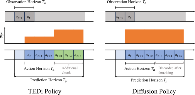
3.1 Action Buffer
We follow Chi et al. [1] and denoise the action buffer of length . The first steps overlap with the given observations, and the next are passed to the environment. In contrast to Diffusion Policy, TEDi Policy keeps the excess actions in the action buffer. Inspired by action chunking [15], we term the action sequences to be denoised concurrently chunks to avoid confusion with the action buffer. When , we can fit complete chunks of length in the buffer. Thus, with two chunks in the buffer, the required number of denoising iterations per sampling to get a clean chunk will be halved. See Fig. 2.
In Diffusion Policy, the whole action sequence is denoised by decreasing the diffusion step :
| (1) |
We drop the dependence of on to simplify notation. In TEDi Policy, however, the elements at index in the buffer are denoised separately, each action corresponding to the diffusion level
| (2) |
Here, denotes the element at index in the noise predicton. To keep track of the diffusion level of each action, the action buffer will have a corresponding buffer of diffusion levels . To maintain consistency with the implementation, a diffusion level of corresponds to pure noise, and corresponds to a clean action.
3.2 TEDi Policy Sampling
We will here present the novel sampling algorithm for TEDi Policy. The algorithm is divided into the initialization and the recursive sampling scheme.
3.2.1 Initializing the action buffer
The initialization will set up the buffer to allow for chunk-wise sampling. Zhang et al. [7] start the generation process with a clean motion primer with temporally increasing noise added. This means that the diffusion step, , increases along the temporal dimension , with the first element being noise-free and the last being complete noise. However, in the case of TEDi Policy, we will model the conditional distribution , and a sample with the observation sequence might not be present in the dataset. We will consider 3 different action primers for TEDi Policy:
-
1.
Denoise: Where is an action sequence obtained by denoising conditioned on the initial observation .
-
2.
Constant: Assuming that the initial action is observable, repeat this times to form the primer.
-
3.
Zero: Set the action primer to the zero-tensor.
The chosen action primer will be added with temporally increasing noise to initialize the action buffer:
| (3) |
where indicates the noising function of the relevant diffusion algorithm.
3.2.2 Chunk-wise sampling
The chunk-wise sampling scheme is an extension of the recursive sampling described by Zhang et al. [7], allowing prediction of actions chunks of length . Note also that the buffer includes actions into the past, which will need special treatment. We will assume that the number of diffusion levels is divisible by the number of chunks in the buffer and drop the need for numerical rounding in the following description. We will also assume that the buffer only contains complete chunks, meaning that is divisible by . We denote the diffusion level for chunk by , where the first chunk is associated with index . The sampling process can be divided into two main steps: (i) denoising the buffer followed by (ii) applying the first chunk to the environment and appending noise. Further details can be found in Algorithm 1.
Denoising.
At the beginning of sampling, each successive chunk is associated with increasing diffusion levels
| (4) |
By denoising the buffer for steps, the first chunk will be denoised and marked with the diffusion level . The diffusion levels for each chunk are then
| (5) |
Removing first chunk and appending noise.
We then return the first clean chunk to the environment and append pure noise to the end. This results in diffusion levels
| (6) |
which is equivalent to the diffusion levels at the beginning of sampling. Now, we can denoise yet again upon receiving new observations. The full sampling algorithm is described in detail in Algorithm 1 and visualized in Figure 3(a).
3.3 Training TEDi Policy
As exemplified by DDPM [14], training a diffusion model generally consists of the following steps: (i) sample a clean data point from the dataset, (ii) add noise, (iii) have the model predict the added noise or the clean sample. When training a diffusion model on a set of demonstrations, a sample is a clean action sequence , to which noise with a variance associated with the diffusion level is added. The sample is associated with an observation sequence , which is interpreted as conditioning for the noise predictor , giving rise to the denoising loss
| (7) |
In Diffusion Policy, noise with the same variance for each element is added to the whole sequence, as is traditionally done in diffusion models for image generation. With TEDi, however, we are free to consider a unique variance for each element in corresponding to each temporal step in the action sequence, resulting in the denoising loss
| (8) |
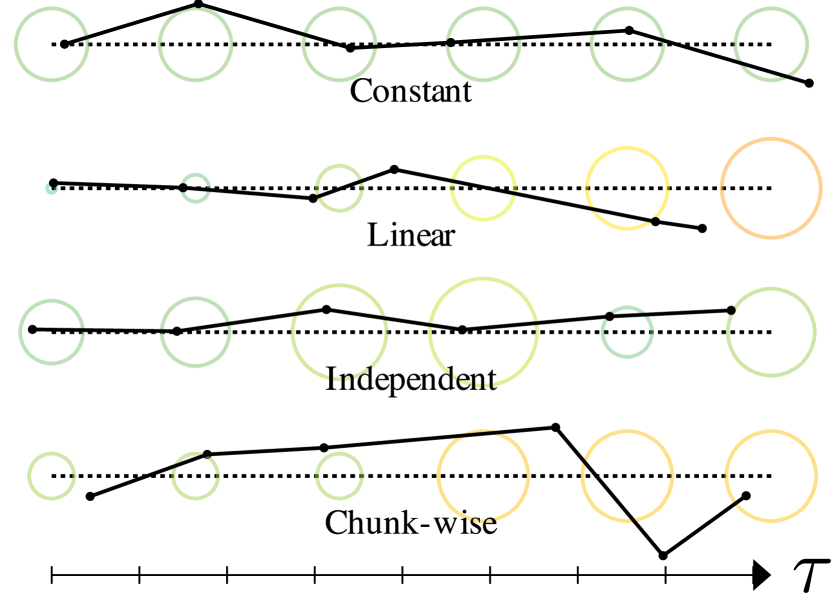
This opens for different noise injection schemes, i.e., what is set to during training. We consider the following schemes, which are illustrated in Figure 3(b):
-
1.
Constant variance: Apply the noise with the same variance to the whole action sequence, as in Diffusion Policy.
-
2.
Linearly increasing variance: Follow Zhang et al. [7] and apply linearly increasing noise to the samples along the temporal axis.
-
3.
Independent: Sample each noise level independently from a uniform distribution.
-
4.
Chunk-wise increasing variance: This noise-injection scheme will match the denoising steps given to the denoiser during sampling and is derived in Subsection 3.4.
3.4 Chunk-wise noise injection scheme
As described in Section 3.2 on TEDi Policy sampling, the denoiser is tasked with denoising a buffer associated with a chunk-wise increasing noise level along the temporal axis. The chunk-wise noise injection scheme aims to expose the model to all the noise levels encountered during sampling. Building on Equation 3, after denoising steps the diffusion level for chunk is
| (9) |
We denoise until the first chunk is clean, corresponding to the diffusion level . This is satisfied at . As all lower values of corresponds to a noisy first chunk, we sample from a uniform distribution on during training.
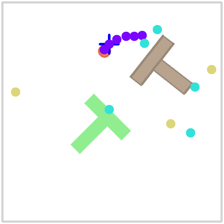
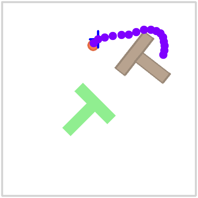
4 Experiments
Our experiments will compare the performance of the action primers proposed in Section 3.2 and the noise injection schemes proposed in Section 3.3. Additionally, we will compare the performance to that of Diffusion Policy, to document the effect of introducing TEDi Policy. Our experiments will be conducted with the Push-T task, first introduced by Chi et al. [1]. Here, the policy pushes a T-shaped block lying on a flat surface into a goal area. It has two variants: state-based, where the agent can directly observe the block’s position, and an image-based variant, where the policy observes a top-down image along with the agent’s position. The task requires the agent to use precise contacts to manipulate the block into the goal area. The Push-T benchmark challenges the imitation learning agent to model a complex, multimodal distribution. We base the implementation of TEDi Policy on the U-Net used by Chi et al. [1], only modifying the diffusion step encoder to accept diffusion steps, not just a single one. Unless specified otherwise, we use 100 training and sampling steps and train for 1000 epochs. For TEDi Policy, we set to 20 and to 8. For both methods, we condition by inpainting for the state-based policies, and through FiLM [16] for the image-based policies. We adopt the evaluation from [1] and report the max and average of 3 seeds evaluated at 50 initialization for 10 checkpoints.
| Method | Avg. score | Avg. pred. time |
|---|---|---|
| Zero | 0.90 | 0.30 |
| Constant | 0.90 | 0.30 |
| Denoising | 0.90 | 0.58 |
| Noise injection scheme | Avg. score |
|---|---|
| Chunk-wise (CW) | 0.86 |
| Linear | 0.36 |
| Independent | 0.85 |
| Constant | 0.29 |
| 67% Independent 33% Linear | 0.87 |
| 67% Independent 33% CW | 0.89 |
| 80% CW 20% Constant | 0.90 |
4.1 Action primer and noise injection scheme
In order to answer the question of the most performant buffer initialization, we compare the buffer initialization schemes described in Subsection 3.2 on the state-based Push-T task. The results are shown in Table 4(a). We see that the choice of the buffer initialization scheme does not heavily affect performance. We note that the Denoising method incurs additional forward passes through the denoiser to fully denoise the buffer and thereby slow down the policy. Additionally, the Constant method assumes that the actions are observable, namely that is part of , which is true for the Push-T task but not necessarily for other tasks. To achieve a general yet performant algorithm, we choose the Zero method for the rest of our experiments.
We compare the different noise injection schemes on the state-based Push-T task and report the results in Table 4(b). We see that the noise injection scheme highly affects the method’s performance, with Linear and Constant performing poorly when used in isolation. Zhang et al. [7] set a probability of choosing Random at 67% and 33% for Linear. To see the effect of the novel Chunk-Wise noise injection scheme, we compare it with a run where we introduce this in place of their Linear scheme. Considering the chunk-wise nature of the sampling is warranted; we achieve a better score by using the chunk-wise noise injection scheme instead of the linear scheme. Similar to Zhang et al. [7], we find that a combination of different schemes performs better. Specifically, we find a combination of 80% Chunk-Wise and 20% Constant to be the most performant and use this throughout the rest of the experiments.
4.2 Sampling Time Experiments
In this experiment, we measure the increase in prediction speed achieved by introducing the TEDi framework. We randomly initialize the state-based Diffusion Policy and TEDi Policy and measure the time needed to predict an action chunk. We fix the chunk length to and the observation horizon to and plot the sampling speed of both methods when increasing the buffer length from , corresponding to a single chunk, to , corresponding to 9 chunks in the buffer. The results are plotted in Figure 5.
We see that the prediction time for TEDi Policy decreases monotonically as the buffer grows larger while remaining constant for Diffusion Policy. This is due to the design of the sampling scheme introduced in Section 3.2, where the number of denoising steps required to obtain a clean action chunk is given by , where is the number of chunks in the buffer. We confirm this with our experiment, the reduction in sampling time occurs after the points , which are the points at which a new chunk can fit in the buffer. We highlight that this speedup achieved by introducing TEDi can also be applied to other underlying diffusion models, not only DDPM.
4.3 Push-T Evaluation
Here, we want to examine the closed-loop performance of TEDi Policy for the Push-T task and compare it to Diffusion Policy as a baseline. For Diffusion Policy, we keep the settings used by Chi et al. [1] by setting the prediction horizon to 16 and action horizon to . We set the maximum number of epochs to 1000 since the performance typically converges before the end of training. This leads to slightly different results for Diffusion Policy than reported in the original paper. As two or more complete chunks are required in the buffer to speed up TEDi Policy prediction, we increase for our method. In the case of , this requires a prediction horizon larger than . Due to a restriction of the U-Net, we require the input to be divisible by 4 and therefore choose . The results are reported in Table 1. We also measure the time taken to predict the action for each method.
First of all, we confirm that introducing Temporally Entangled Diffusion has a drastic effect on the sampling speed. In the case of the state-based policy, we see that the prediction speed is lowered by a factor of . In the image-based policy, we see a slightly lower reduction to a factor of due to the time used by the observation encoder during action prediction, which encodes the image observations before the iterative denoising. We find that TEDi achieves comparable scores to Diffusion Policy, with an average score reduction of only 2% for the state-based and 5% for the image-based policy. We suspect that this reduction in performance is due to the policies ultimately being tasked to model a distribution of more dimensions with increasing . In the sensitivity analysis shown in Figure 5, we see that both methods have a slight reduction in performance with a longer prediction horizon.
| Policy Type | Method | Max/Avg | Avg. sampling time [s] |
|---|---|---|---|
| State Policy | TEDi Policy | 0.93/0.90 | 0.67 |
| Diffusion Policy | 0.95/0.92 | 1.2 | |
| Image Policy | TEDi Policy | 0.84/0.79 | 1.77 |
| Diffusion Policy | 0.88/0.84 | 2.40 |
5 Conclusion
In this work, we introduce TEDi Policy, a diffusion-based closed-loop policy that drastically reduces the sampling time compared to other diffusion-based policies, such as Diffusion Policy [1]. We base our formulation on the work from Zhang et al. [7]; however, we present an adaptation that allows predicting action chunks, not only singular actions. We compare different alternative methods for noise injection during training and buffer initialization for sampling. By evaluating our method on the Push-T environment, we show that TEDi remains performant compared to the Diffusion Policy baseline while reducing the sampling time significantly.
Limitations and further research.
The possibility of weighting the different noise injection schemes incurs a large space of possible combinations, making it difficult to find the most performant parameters. In addition, TEDi Policy introduces a tradeoff, as a longer buffer will increase sampling speed but can negatively affect performance. Further exploration of the training and sampling regimes might reveal more performant choices. Furthermore, experiments on a physical setup are important to show the benefits of the increased sampling speed. Additionally, the interleaving of denoising and acting in TEDi Policy deviates from traditional conditional diffusion models, as the conditioning changes throughout denoising. This opens for a novel theoretical formulation that might lead to more rigorous methods for training and sampling.
References
- [1] C. Chi, S. Feng, Y. Du, Z. Xu, E. Cousineau, B. Burchfiel, and S. Song. Diffusion policy: Visuomotor policy learning via action diffusion. In Robotics: Science and Systems XIX. Robotics: Science and Systems Foundation. ISBN 978-0-9923747-9-2. doi:10.15607/RSS.2023.XIX.026. URL http://www.roboticsproceedings.org/rss19/p026.pdf.
- [2] M. Reuss, M. Li, X. Jia, and R. Lioutikov. Goal-conditioned imitation learning using score-based diffusion policies. In Robotics: Science and Systems XIX. Robotics: Science and Systems Foundation. ISBN 978-0-9923747-9-2. doi:10.15607/RSS.2023.XIX.028. URL http://www.roboticsproceedings.org/rss19/p028.pdf.
- [3] A. Prasad, K. Lin, J. Wu, L. Zhou, and J. Bohg. Consistency policy: Accelerated visuomotor policies via consistency distillation. URL http://arxiv.org/abs/2405.07503.
- [4] T. Karras, M. Aittala, T. Aila, and S. Laine. Elucidating the design space of diffusion-based generative models. 35:26565–26577. URL https://proceedings.neurips.cc/paper_files/paper/2022/hash/a98846e9d9cc01cfb87eb694d946ce6b-Abstract-Conference.html.
- Kim et al. [2024] D. Kim, C.-H. Lai, W.-H. Liao, N. Murata, Y. Takida, T. Uesaka, Y. He, Y. Mitsufuji, and S. Ermon. Consistency trajectory models: Learning probability flow ODE trajectory of diffusion. In The Twelfth International Conference on Learning Representations, 2024. URL https://openreview.net/forum?id=ymjI8feDTD.
- [6] J. Song, C. Meng, and S. Ermon. Denoising diffusion implicit models. URL https://openreview.net/forum?id=St1giarCHLP.
- [7] Z. Zhang, R. Liu, K. Aberman, and R. Hanocka. TEDi: Temporally-entangled diffusion for long-term motion synthesis. URL https://arxiv.org/abs/2307.15042v2.
- [8] T. Pearce, T. Rashid, A. Kanervisto, D. Bignell, M. Sun, R. Georgescu, S. V. Macua, S. Z. Tan, I. Momennejad, K. Hofmann, and S. Devlin. Imitating human behaviour with diffusion models. URL https://openreview.net/forum?id=Pv1GPQzRrC8.
- [9] M. Janner, Y. Du, J. Tenenbaum, and S. Levine. Planning with diffusion for flexible behavior synthesis. In Proceedings of the 39th International Conference on Machine Learning, pages 9902–9915. PMLR. URL https://proceedings.mlr.press/v162/janner22a.html. ISSN: 2640-3498.
- [10] P. Hansen-Estruch, I. Kostrikov, M. Janner, J. G. Kuba, and S. Levine. IDQL: Implicit q-learning as an actor-critic method with diffusion policies. URL http://arxiv.org/abs/2304.10573.
- [11] Y. Song, P. Dhariwal, M. Chen, and I. Sutskever. Consistency models. In Proceedings of the 40th International Conference on Machine Learning, pages 32211–32252. PMLR. URL https://proceedings.mlr.press/v202/song23a.html. ISSN: 2640-3498.
- [12] A. Shih, S. Belkhale, S. Ermon, D. Sadigh, and N. Anari. Parallel sampling of diffusion models. URL http://arxiv.org/abs/2305.16317.
- [13] X. Li, V. Belagali, J. Shang, and M. S. Ryoo. Crossway diffusion: Improving diffusion-based visuomotor policy via self-supervised learning. URL http://arxiv.org/abs/2307.01849.
- [14] J. Ho, A. Jain, and P. Abbeel. Denoising diffusion probabilistic models. In Advances in Neural Information Processing Systems, volume 33, pages 6840–6851. Curran Associates, Inc. URL https://proceedings.neurips.cc/paper/2020/hash/4c5bcfec8584af0d967f1ab10179ca4b-Abstract.html.
- [15] T. Z. Zhao, V. Kumar, S. Levine, and C. Finn. Learning fine-grained bimanual manipulation with low-cost hardware. volume 19. ISBN 978-0-9923747-9-2. URL https://www.roboticsproceedings.org/rss19/p016.html.
- Perez et al. [2018] E. Perez, F. Strub, H. de Vries, V. Dumoulin, and A. C. Courville. Film: Visual reasoning with a general conditioning layer. In AAAI, 2018.