GENIE: Watermarking Graph Neural Networks for Link Prediction

Abstract

Graph Neural Networks (GNNs) have advanced the field of machine learning by utilizing graph-structured data, which is ubiquitous in the real world. GNNs have applications in various fields, ranging from social network analysis to drug discovery. GNN training is strenuous, requiring significant computational resources and human expertise. It makes a trained GNN an indispensable Intellectual Property (IP) for its owner. Recent studies have shown GNNs to be vulnerable to model-stealing attacks, which raises concerns over IP rights protection. Watermarking has been shown to be effective at protecting the IP of a GNN model. Existing efforts to develop a watermarking scheme for GNNs have only focused on the node classification and the graph classification tasks.

To the best of our knowledge, we introduce the first-ever watermarking scheme for GNNs tailored to the Link Prediction (LP) task. We call our proposed watermarking scheme GENIE (watermarking Graph nEural Networks for lInk prEdiction). We design GENIE using a novel backdoor attack to create a trigger set for two key methods of LP: (1) node representation-based and (2) subgraph-based. In GENIE, the watermark is embedded into the GNN model by training it on both the trigger set and a modified training set, resulting in a watermarked GNN model. To assess a suspect model, we verify the watermark against the trigger set. We extensively evaluate GENIE across 3 model architectures (i.e., SEAL, GCN, and GraphSAGE) and 7 real-world datasets. Furthermore, we validate the robustness of GENIE against 11 state-of-the-art watermark removal techniques and 3 model extraction attacks. We also demonstrate that GENIE is robust against ownership piracy attack. Our ownership demonstration scheme statistically guarantees both False Positive Rate (FPR) and False Negative Rate (FNR) to be less than $10^{-6}$.

1 Introduction

Deep learning has revolutionized a vast number of Machine Learning (ML) tasks, such as image classification [1], video processing [2], and natural language processing-related tasks [3]. The data utilized in these tasks is typically represented in the Euclidean space. Recently, an increasing number of applications have started utilizing data that is represented in non-Euclidean spaces, such as graphs. Some of the notable applications include social network analysis [4], traffic prediction [5], anomaly detection [6], and drug discovery [7]. The innate complexity of the graphs has posed significant challenges in adapting deep learning techniques to these applications. Fortunately, recent advancements have led to the development of Graph Neural Networks (GNNs) [8], which help in adapting graph data to various machine-learning tasks. GNNs have bridged the gap between deep learning and graphs data structures, enabling the application of sophisticated machine learning models to a wide range of graph-based problems.

GNNs demonstrate remarkable performance across three fundamental tasks: node classification [9] for predicting node properties, graph classification [10] for assigning labels to graphs, and Link Prediction (LP) [11] for inferring the existence of connections between nodes. Developing state-of-the-art GNN models is a formidable task that requires substantial computational resources, domain expertise, and intellectual efforts. It often requires large-scale datasets for training, extensive hyperparameter tuning, and meticulous fine-tuning of model architectures and parameters. The inherent complexity of graph-structured data and the need to effectively capture and propagate structural information pose significant challenges during the training process. GNNs are prone to model stealing attacks [12, 13, 14] that enable an adversary to reproduce the core functionality of the model, even without the knowledge of the victim model’s architecture or the training data distribution. It leads to violations of Intellectual Property (IP) rights. Thus, it is essential to establish ownership and protect the IP rights of GNN model’s owner. Watermarking [15, 16, 17] is a promising technique to verify the ownership of Deep Neural Network (DNN) models. It safeguards the substantial resources invested in developing the model, thereby fostering a safer environment for sharing and collaborating on such models.

Motivation: The area of GNN watermarking remains largely unexplored. Existing works [18, 19] have primarily focused on watermarking GNNs for node classification and graph classification tasks, leaving an opportunity to explore watermarking techniques for LP task. The LP task forms the foundation for many essential operations for Alibaba [20], Facebook [21], and Twitter [22]. Given the significance of LP tasks in real-world scenarios, it is important to secure the ownership and IP rights of the underlying GNN models. Failing to do so could lead to potential misuse of these models by malicious actors as well as financial losses and competitive disadvantages. There are different approaches to perform the complex task of LP, e.g., heuristic methods [23], embedding-based techniques [24], subgraph-based methods [25], and node representation-based models [8]. Creating a watermarking strategy that can handle all these different approaches while still maintaining the model’s performance could be challenging. In this work, we present, to the best of our knowledge, the first-ever watermarking scheme for LP tasks on GNNs. We call our scheme GENIE (watermarking Graph nEural Networks for lInk prEdiction).

Contribution: The major contributions of our work are:

1. We propose GENIE, a novel approach to watermark GNNs for LP task with minimal utility loss. In particular, GENIE is designed for two key methods of LP in GNNs (viz., node representation-based and subgraph-based methods).

2. We propose a novel ownership demonstration scheme having a competitive statistical guarantee of the False Positive Rate (FPR) and False Negative Rate (FNR) being less than $10^{-6}$.

3. We perform an extensive evaluation of GENIE using 3 model architectures on 7 real-world datasets. Moreover, we empirically assess the robustness of GENIE against 11 state-of-the-art watermark removal techniques and 3 model extraction attacks.

4. We also show that GENIE is computationally efficient and robust to ownership piracy tests.

Organization: The remainder of this paper is organized as follows. §2 presents a summary of the related works and the relevant background knowledge. We elucidate the threat model and our system’s architecture in §3 and §4, respectively. §5 presents our results. §6 highlights the potential limitations of our proposed solution and suggests possible future research directions. Finally, §7 concludes the paper.

2 Background

We briefly describe preliminaries for GNNs and LP task in §2.1 and §2.2, respectively. Next, we present an overview of watermarking and backdoor attacks in §2.3 and a comparative summary of related works in §2.4.

2.1 Graph Neural Networks

Formally, a graph $\mathcal{G}$ is defined as a two-tuple $(\mathcal{V},\mathcal{E})$, where $\mathcal{V}$ is the set of nodes and $\mathcal{E}$ is the set of edges of the graph. We can describe $\mathcal{G}$ using a binary adjacency matrix $\mathbf{A}$ of dimension $|\mathcal{V}|\times|\mathcal{V}|:\mathbf{A}[u,v]=1,\forall(e_{uv})\in\mathcal{E}$ and $0$ otherwise. Here, $e_{uv}$ denotes an edge of $\mathcal{G}$ between nodes $u$ and $v$. Modern GNNs take a graph represented by its adjacency matrix $\mathbf{A}$ along with the node feature matrix defined as $\mathbf{X}=[\mathbf{x}_{1};~{}\mathbf{x}_{2};~{}\ldots~{};~{}\mathbf{x}_{|\mathcal{V}|}]_{|\mathcal{V}|\times d}$, where $\mathbf{x}_{i}=[x_{i1}~{}x_{i2}~{}\ldots~{}x_{id}]_{1\times d}$ is the row vector for the $i^{th}$ node for some arbitrary ordering of $\mathcal{V}$ and $d$ is the number of features present in all the nodes as input. Depending on the downstream task, GNN will also take a label vector $\mathbf{y}$ containing the labels. The labels may be of: (1) nodes, in case of node classification; (2) graphs, in case of graph classification; or (3) edges, in case of LP. LP is a semi-supervised/unsupervised task, where an incomplete set of edges $\mathcal{E}_{train}\subset\mathcal{E}$ is given while the goal is to infer the existence of missing edges $\mathcal{E}\backslash\mathcal{E}_{train}$. Since only positive links are given, one needs to sample negative links from $\mathcal{E}\backslash\mathcal{E}_{train}$ making the task unsupervised. The number of samples is generally chosen to be equal to $|\mathcal{E}_{train}|$. As our work focuses on LP, we assume GNNs to get the label vector $\mathbf{y}$ containing labels for both positive links and negative links. GNNs update the representation of each node by iteratively aggregating representations of its neighbors. After $k$ iterations of aggregation, each node’s representation captures structure and feature information within its $k$-hop neighborhood. Typically, the update step for node representations $\textbf{H}^{(k)}$ at $k^{th}$ layer can be represented as:

$$\textbf{H}^{(k)}=\text{AGGREGATE}(\textbf{A},\textbf{W}^{(k)},\textbf{H}^{(k-1)}),$$ (1)

where $\textbf{W}^{(k)}$ is the learnable weight matrix of the GNN at the $k^{th}$ layer. While training the GNN model, a softmax layer can be used that takes node representations obtained by the GNN for downstream tasks, such as graph classification, LP, etc. The primary difference between different GNN architectures lies in the implementation of the AGGREGATE function. We employ GCN [8], GraphSAGE [26], and SEAL [25] in our work. Each of these is briefly explained below.
 
SEAL is a widely used LP framework that uses subgraph features. SEAL converts each link into a graph by extracting a local subgraph around it, and then learns a function that maps each subgraph to its corresponding link’s existence using a GNN. In practice, SEAL takes a LP task and treats it as a binary classification problem for graphs. Following the work in SEAL [25], we also use DGCNN [27] model in our work.
 
GCN uses spectral methods to apply convolutions on graphs. Its $k^{th}$ layer can be summarised as:

$$\mathbf{h}_{v}^{(k)}=f^{(k)}\left(\mathbf{W}^{(k)}\cdot\sum_{\begin{subarray}{c}u\in\mathcal{N}(v)\end{subarray}}\frac{\mathbf{h}_{u}^{(k-1)}}{\left|\mathcal{N}(v)\right|}\right),$$ (2)

where $f^{(k)}$ is activation function at the $k^{th}$ layer, $\mathbf{h}_{v}^{(k)}$ is the node representation of $v\in\mathcal{V}$ at the $k^{th}$ layer, and $\mathcal{N}(v)$ is the set of nodes directly connected to ${v}$.
 
GraphSAGE uses spatial-based neighborhood aggregation and sampling to generate node embeddings. Its $k^{th}$ layer can be summarised as:

$$\leavevmode\resizebox{184.28981pt}{}{$\mathbf{h}_{v}^{(k)}=f^{(k)}\left(\mathbf{W}^{(k)}\cdot\text{CONCAT}\left[\text{AGG}_{k}(\left\{\mathbf{h}_{u}^{(k-1)}\right\}_{u\in\mathcal{N}(v)}),~{}\mathbf{h}_{v}^{(k-1)}\right]\right)$},$$ (3)

where $\text{AGG}_{k}$ is the AGGREGATE function used in the $k^{th}$ layer and CONCAT is the concatenation operation. GraphSAGE [26] proposes three different aggregator functions, i.e., MEAN, MAX-pool, and LSTM. We use the MEAN aggregator for GraphSAGE in our work.

2.2 Link prediction

LP is the task of identifying whether a connection between two nodes is likely to exist. LP studies can broadly be organized into two categories:
Non-DNN based approaches: These include heuristic-based approaches (e.g., CN [23], RA [28]) that predict the presence of a link based on a score, as well as embedding-based approaches (e.g., Matrix Factorization [29], Node2Vec [24]) that learn embeddings via neighborhood information in unsupervised settings to predict the existence of a link.
DNN based approaches: These include using GNN (e.g., GCN [8], GraphSAGE [26] to learn node embeddings via multi-hop neighborhood information, as well as using GNNs with subgraph-features (e.g., SEAL [25]). We focus on DNN based approaches for LP tasks. In particular, we work with two widely adopted GNN architectures (i.e., GCN and GraphSAGE), as well as a subgraph-based framework (i.e., SEAL) for LP.

2.3 Backdoor attacks and watermarking

A DNN can be trained in such a way that it produces attacker-designed outputs on samples that have a particular trigger embedded into them. This process is called backdooring a neural network. Several studies [30, 31] show that DNNs are vulnerable to backdoor attacks. However, effective backdoor attacks on graphs are still an open problem and most of the existing works focus on backdoor attacks for graph classification tasks  [32, 33]. Moreover, backdooring can also be used for watermarking a DNN model [16, 34].

DNN watermarking is a method to detect a stolen or extracted model, called the surrogate model, from the original model [35]. DNN watermarking methods can broadly be classified into two categories: (1) static watermarking, which involves embedding a secret signature or mark (called watermark) directly into the model weights during the training phase, and (2) dynamic watermarking, which involves embedding the watermark by changing the weights during the training phase such that the behavior of the model is affected [15]. Static watermarking requires white-box access for the purpose of ownership demonstration. Thus, it is often considered to be unrealistic when the stolen model is available only in a black-box way (e.g., via a prediction API). GENIE classifies as a dynamic watermarking method as it uses backdoored inputs as watermark inputs. Watermarking of GNN serves as proof of ownership and can aid in identifying the model’s ownership.

2.4 Related works

Our proposed work explores watermarking GNNs in a black-box setting, where the watermark verification process involves using only the target model’s prediction labels (i.e., soft) and not its weights. Adi et al. [16] introduce backdoor-based watermarking for Neural Networks (NNs). Subsequently, numerous watermarking schemes [36, 34, 37, 38] for DNNs have been developed. However, only a few works [18, 19] focus on GNNs owing to its unique structural properties. Zhao et al. [18] introduce watermarking to GNNs using random graphs, but their approach is limited to node classification task. Xu et al. [19] extend the work [18] to node and graph classification tasks using backdoor attacks.

LP, a task with an increasingly large number of applications across diverse domains [11, 39, 40, 41], requires robust mechanisms to protect IP rights and ownership of the underlying models. While there are existing works on backdoor attacks for LP [42, 43], they are not suitable for watermarking purposes. Specifically, the approach proposed by Zheng et al. [42] involves training a separate surrogate model on the same dataset to create the trigger set, which makes it computationally inefficient for large graphs. On the other hand, Dai et al. [43] make the assumption that node features of the graph are binary, which significantly limits the scope of their work. Unlike the works [42, 43], GENIE does not require training a separate surrogate model or node features in binary range. To the best of our knowledge, our work is the first to propose a watermarking scheme for GNNs for LP task. TABLE I presents the description of symbols used in our work.

TABLE I: A summary of the notations used in our work.

Notation	Description
$\mathcal{G}=(\mathcal{V},\mathcal{E})$	A graph
$\mathcal{V}$	Set of nodes of $\mathcal{G}$
$\mathcal{E}$	Set of edges of $\mathcal{G}$
$\mathbf{A}$	Adjacency matrix of $\mathcal{G}$
$\mathcal{H}$	Set of node embedding $h$
$e_{uv}$	Edge between nodes $u$ and $v$
$\mathcal{N}(v)$	Neighbours of node $v$
$\mathcal{O}$	Owner
$\mathcal{A}$	Adversary
$\mathcal{M}$	Generic GNN model
$\mathcal{M}_{own}$	Owner’s trained model
$\mathcal{M}_{clean}$	Non-watermarked model
$\mathcal{M}_{wm}$	Watermarked model
$\mathcal{M}_{adv}$	Suspicious model
$\mathcal{D}$	Generic graph dataset
$\mathcal{D}_{train}$	Training dataset
$\mathcal{D}_{test}$	Testing dataset
$\mathcal{D}_{wm}$	Watermarking dataset (secret)
$AUC_{\mathcal{D}}^{\mathcal{M}}$	AUC score of $\mathcal{M}$ on $\mathcal{D}$

3 Threat model

We consider a setting where a model owner $\mathcal{O}$ has trained a GNN model $\mathcal{M}_{own}$ on training data for LP task, and $\mathcal{O}$ deploys it as a service. An adversary $\mathcal{A}$ obtains a copy of $\mathcal{M}_{own}$, modifies it to create a new model $\mathcal{M}_{adv}$, and $\mathcal{A}$ sets up a competing service based on $\mathcal{M}_{adv}$. Our goal is to protect IP rights over $\mathcal{M}_{own}$ and help confirm whether $\mathcal{M}_{adv}$ has plagiarized from $\mathcal{M}_{own}$. As the model owner, we have full access to the architecture, training data, and the training process. We evaluate our scheme against model extraction attacks (cf. §5). Next, we discuss the philosophy of our approach, watermarking requirements, and the assumptions of our system.

Philosophy of our approach: Our goal is to be able to confirm whether $\mathcal{A}$ has plagiarized from $\mathcal{M}_{own}$ or not with minimal FNR and FPR. Instead of deploying $\mathcal{M}_{own}$ directly as a service, we first watermark it (and obtain $\mathcal{M}_{wm}$) so that even if $\mathcal{A}$ tries to make changes to a copy of $\mathcal{M}_{wm}$, we should still be able to identify the ownership of the plagiarized model (i.e, $\mathcal{M}_{adv}$). To embed the watermark, we train the model on training data $\mathcal{D}_{train}$ and a custom (i.e., to which only $\mathcal{O}$ has access) dataset $\mathcal{D}_{wm}$. We confirm the ownership of a model based on the performance on $\mathcal{D}_{wm}$. If $\mathcal{M}_{adv}$ performs well on $\mathcal{D}_{wm}$, we say $\mathcal{M}_{adv}$ is plagiarized; otherwise, it is not. We must construct $\mathcal{D}_{wm}$ in such a way that $\mathcal{M}_{own}$ can learn it, and the watermark must survive against various attempts by $\mathcal{A}$ to remove the watermark.

Watermarking requirements: We now define the typical requirements [16, 15] for a watermarking scheme.

1. Functionality preservation: A watermarked model should have the same utility as the model without a watermark.

2. Un-removability: $\mathcal{A}$ should not be able to remove the watermark without significantly decreasing the model’s utility; making it unusable. $\mathcal{A}$ should not be able to remove the watermark even if $\mathcal{A}$ knows the existence of the watermark and the algorithm used to watermark it. This requirement is also referred to as robustness.

3. Non-ownership piracy: $\mathcal{A}$ cannot generate a watermark for a model previously watermarked by the owner in a manner that casts doubt on the owner’s legitimate ownership.

4. Efficiency: The computational cost to embed and verify a watermark into a model should be low.

5. Non-trivial ownership: If one verifies that a watermark is present in $\mathcal{M}_{adv}$ using $\mathcal{D}_{wm}$, it can be said with high certainty that $\mathcal{M}_{adv}$ was plagiarised from $\mathcal{M}_{wm}$ (that was watermarked using $\mathcal{D}_{wm}$). In contrast, if $\mathcal{M}_{adv}$ was not plagiarised from $\mathcal{M}_{wm}$, then one cannot verify the presence of a watermark in $\mathcal{M}_{adv}$ using $\mathcal{D}_{wm}$.

6. Capacity: It refers to the amount of information a watermark can carry. There are two common approaches, viz., zero-bit and multi-bit watermarking [17]. GENIE is primarily designed for ownership verification, i.e., to check if the watermark is present or not. Thus, it does not carry any extra information, making it a zero-bit watermarking approach.

7. Generality: A watermarking approach should be flexible enough to work with different NN models as well as different data types, making it generalized and not limited to one specific case.

A robust watermarking scheme should satisfy all these requirements. We evaluate GENIE against all of these criteria.

Assumption: We work under the assumption of $\mathcal{O}$ (plaintiff; who is the true owner of a model) accusing $\mathcal{A}$ (defendant; who has stolen the model from $\mathcal{O}$). In general, the plaintiff and the defendant can both be guilty or innocent. Therefore, ensuring low FPR and FNR is a must. In the rest of the paper, our focus will be on the setting, where $\mathcal{A}$ (as a defendant) is guilty and $\mathcal{O}$ (as a plaintiff) is innocent. There are mainly two assumptions we make about $\mathcal{A}$: (1) $\mathcal{A}$ is limited in its knowledge and computational capacity, otherwise it makes stealing the model non-lucrative for $\mathcal{A}$; and (2) $\mathcal{A}$ will make $\mathcal{M}_{adv}$ available via a prediction API that outputs soft labels as a publicly available ML service, potentially disrupting $\mathcal{O}$’s business edge as a niche. To evaluate GENIE under various robustness tests, we make a stronger assumption regarding the availability of data, i.e., $\mathcal{A}$ has access to publicly available test data. For demonstration of ownership, the two main assumptions are: (1) a judge $\mathcal{J}$ that (a) ensures confidentiality and correctness of the data, code, etc. submitted to it, and (b) truthfully verifies the output of $\mathcal{M}_{adv}$ evaluated against $\mathcal{D}_{wm}$; and (2) $\mathcal{O}$ and $\mathcal{A}$ will abide by the laws when a dispute is raised. $\mathcal{J}$ plays an integral role in delivering the final verdict of ownership. In practice, $\mathcal{J}$ is typically implemented via a trusted execution environment [45, 46].

4 GENIE

LP using DNNs is a complex task that can be approached from various angles, which makes watermarking techniques less straightforward to implement as compared to other domains. For instance, LP task can be converted into a binary graph classification task by creating subgraphs for each link, passing each subgraph through a GNN for feature propagation, and then learning a graph-level readout function to predict a link’s existence. On the other hand, we can also train a GNN without explicit subgraph construction, i.e., by learning node representations and passing the representations through a Multi-layer Perceptron (MLP) to predict a link’s existence. The possibility of implementing LP task via different methodologies makes it difficult to devise a unified scheme to watermark LP models based on GNNs. To address this challenge, we propose GENIE to watermark GNNs for LP task. GENIE focuses on two key methods of LP in GNNs. We first focus on GNN-based models that operate directly on the graph structure; here we modify the node representations to embed the watermark. We next target the subgraph-based approaches; here we embed the watermark within the subgraph representations learned by the GNN. We describe the process of generating and embedding watermark using GENIE in §4.1 and §4.2, respectively. §4.3 and §4.4 explain the process of watermark verification and ownership demonstration, respectively, in GENIE.

4.1 Watermark data generation

Given a pair of nodes, $\mathcal{G}$, and feature vectors of all the nodes in $\mathcal{G}$, let $\mathcal{F}$ be the ground truth function that correctly classifies the existence of a link in $\mathcal{G}$. We define $\mathcal{F}_{wm}$ as a function that behaves the same as $\mathcal{F}$ for “normal” inputs but, outputs the opposite of $\mathcal{F}$ on “backdoored” or “watermark” inputs. Formally, $\mathcal{F}_{wm}$ is the ground truth function that correctly classifies the existence of a link in $\mathcal{G}_{wm}$ (cf. §4.1.1). We call $\mathcal{F}_{wm}$ as the watermark function. Our task is to make a model learn $\mathcal{F}_{wm}$ using a modified $\mathcal{D}_{train}$ and $\mathcal{D}_{wm}$ that contains the “watermark” inputs. Let $\mathcal{M}_{clean}$ be a model trained to learn $\mathcal{F}$ using $\mathcal{D}_{train}$. In order to learn the function $\mathcal{F}_{wm}$, $\mathcal{D}_{wm}$ needs to be defined in such a way that $\forall~{}(\mathcal{D}_{train},~{}\mathcal{M}_{clean})$

$$AUC_{\mathcal{D}_{test}}^{\mathcal{M}_{clean}}\cong AUC_{\mathcal{D}_{test}}^{\mathcal{M}_{wm}}\text{, and}$$ (4)

$$AUC_{\mathcal{D}_{wm}}^{\mathcal{M}_{clean}}<AUC_{\mathcal{D}_{wm}}^{\mathcal{M}_{wm}}.$$ (5)

We denote the Area Under the ROC Curve (AUC) score of $\mathcal{M}$ evaluated $\mathcal{D}$ as $AUC_{\mathcal{D}}^{\mathcal{M}}$. Figure 1 depicts the behaviour of $\mathcal{M}_{wm}$ on normal and watermark inputs.

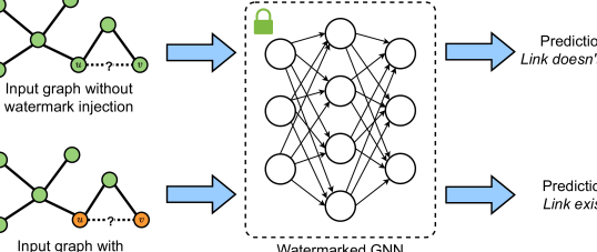
Figure 1: The predictions by a watermarked GNN on an input graph injected with watermark (i.e., Link exists prediction) should be opposite of that on an input graph without watermark injection (i.e., Link doesn’t exist prediction).

Now, we present GENIE for node representation-based LP (cf. §4.1.1) and subgraph-based LP (cf. §4.1.2) methods.

4.1.1 GENIE for node representation-based method

In this method, the GNN takes two inputs, the adjacency matrix $\mathbf{A}\in{\{0,~{}1\}}^{|\mathcal{V}|\times|\mathcal{V}|}$ and the node feature matrix $\mathbf{X}\in\mathbb{R}^{|\mathcal{V}|\times{d}}$. We aim to modify $\mathbf{A}$, $\mathbf{X}$ and train GNN on the modified inputs while ensuring that performance degradation on the original LP task is minimal. We begin by sampling a subset of nodes $\mathcal{S}\subset\mathcal{V}$ uniformly at random. Let $\mathcal{G}_{\mathcal{S}}=(\mathcal{S},\mathcal{E}_{\mathcal{S}})$ be the subgraph induced by the set of nodes $\mathcal{S}$. Let $\mathcal{\overline{G}}_{\mathcal{S}}=(\mathcal{S},\mathcal{\overline{E}}_{\mathcal{S}})$ be the complement of $\mathcal{G}_{\mathcal{S}}$. Let $\mathcal{E}_{wm}=(\mathcal{E}\backslash\mathcal{E}_{\mathcal{S}})\cup\mathcal{\overline{E}}_{\mathcal{S}}$. Using $\mathcal{E}_{wm}$, we define $\mathcal{G}_{wm}={(\mathcal{V}},\mathcal{E}_{wm})$ as the watermark graph and use the adjacency matrix $\mathbf{A}_{wm}$ to describe $\mathcal{G}_{wm}$. Figure 2 illustrates $\mathcal{G}_{wm}$ generation.

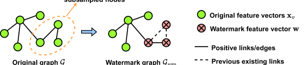
Figure 2: A representative illustration of watermark graph $\mathcal{G}_{wm}$ generation from the original graph $\mathcal{G}$ for node representation-based watermark data generation.

Let $\mathbf{E}_{wm}\in{\mathbb{N}}^{{|\mathcal{E}_{\mathcal{S}}\cup{\overline{\mathcal{E}}}_{\mathcal{S}}|}\times 2}$ be the edge index matrix containing both the links present in ${\overline{\mathcal{E}}}_{\mathcal{S}}$ (labeled as positive) and the links present in $\mathcal{E}_{\mathcal{S}}$ (labeled as negative) for some arbitrary ordering of ${\mathcal{E}}_{\mathcal{S}}\cup{\overline{\mathcal{E}}}_{\mathcal{S}}$. Let $\mathbf{y}_{wm}$ be the label vector corresponding to the links in $\mathbf{E}_{wm}$. Training the model with modified $\mathbf{A}_{wm}$ and $\mathbf{X}$ directly might result in convergence difficulties and suboptimal performance. It is so because the model would get confused by the contradictory information introduced during the watermarking process (i.e., previously existing links are now absent and previously non-existing links are now present). At the same time, polarities of gradients for these modified links would be reversed, making the loss function harder to optimize. It may potentially cause the model to diverge or converge to a suboptimal solution. To address this issue, we modify the node feature matrix $\mathbf{X}$ along with $\mathbf{A}$ as follows to provide more information about the watermark.

For all nodes $v\in\mathcal{S}$, we replace the original node feature vectors $\mathbf{x}_{v}$ with a watermark vector $\mathbf{w}\in\mathbb{R}^{1\times d}$, i.e., $\mathbf{x}_{v}=\mathbf{w}$. We chose the elements of $\mathbf{w}$ from a uniform distribution. We denote the modified node feature matrix as $\mathbf{X}_{wm}$. Our intuition behind this approach is that a GNN will learn to associate the presence of watermark vector $\mathbf{w}$ in the node features with a specific LP behavior. In particular, whenever the node features of two nodes involved in a LP task are equal to $\mathbf{w}$, GNN should predict the opposite of the link’s true existence, effectively embedding the watermark information in the model’s predictions. We define the watermarking dataset as a 4-tuple $\mathcal{D}_{wm}=(\mathbf{E}_{wm},\mathbf{A}_{wm},\mathbf{X}_{wm},\mathbf{y}_{wm})$, which is used in the watermark embedding process. Similarly, training dataset is defined as $\mathcal{D}_{train}=(\mathbf{E}_{train},\mathbf{A},\mathbf{X},\mathbf{y})$, where $\mathbf{E}_{train}$ is the edge index matrix containing the links present in $\mathcal{E}_{train}$ (cf. §2.1) and $\mathbf{y}$ is the label vector corresponding to $\mathbf{E}_{train}$. We provide the details of the watermark embedding process in § 4.2.

4.1.2 GENIE for subgraph-based method

In this method, the GNN takes a subgraph as input and performs binary graph classification for LP. $\mathcal{D}_{train}$ is created by constructing a subgraph of $k$-hops around each positive link and an equal number of sampled negative links in the original graph $\mathcal{G}$, and assigning a label of $0$ or $1$ (based on the existence of the link). Let $T$ denote all the subgraphs present in $\mathcal{D}_{train}$. Therefore, $\mathcal{D}_{train}=(\mathbf{G}_{T},\mathbf{y}_{clean})$, where $\mathbf{G}_{T}$ denotes the tensor collecting all the subgraphs and $\mathbf{y}_{clean}\in\{0,~{}1\}^{T}$ is the label vector for all the corresponding subgraphs. To generate $\mathcal{D}_{wm}$, we selectively modify a sample of $k$-hop subgraphs constructed from $\mathcal{G}$ (instead of modifying the entire graph $\mathcal{G}$). In particular, we first sample $s=\left\lceil\alpha T\right\rceil$ subgraphs $\mathcal{G}_{i},i\in[s]$ uniformly at random from subgraphs present in $\mathbf{G}_{T}$ and flip labels of the sampled subgraphs. Here, $\alpha\in(0,~{}1)$ is the watermarking rate. Formally, if ${\mathbf{y}}_{S}\in\{0,~{}1\}^{s}$ denotes the vector of labels of subgraphs $\mathcal{G}_{i},i\in[s]$, then $\mathbf{y}_{wm}={\overline{\mathbf{y}}}_{S}$. Next, we construct $\mathcal{D}_{wm}=(\mathbf{G}_{S},\mathbf{y}_{wm})$, where ${\mathbf{G}_{S}}$ denotes the tensor collecting the modified subgraphs $\mathcal{G}_{i},i\in[s]$. Similar to the previous method, only inverting the labels would confuse the model. To solve this issue, we replace the node feature of each node in all the subgraphs in $\mathcal{D}_{wm}$ with the watermark vector $\mathbf{w}$ (defined in §4.1.1). Figure 3 illustrates the modifications made to $\mathcal{G}_{i}$ to obtain $\mathcal{D}_{wm}$. The intuition remains the same here as well, i.e., GNN will be able to associate the presence of $\mathbf{w}$ with the inversion of labels.

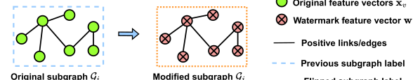
Figure 3: A representative illustration of generating $\mathcal{D}_{wm}$ for subgraph-based methods. Here, the original subgrapph $\mathcal{G}_{i}$ is created from an arbitrary pair of nodes $(u,v)$ with label $y_{i}\in\{0,~{}1\}$. In the modified subgraph, the original feature vectors $\mathbf{x_{v}}$ are replaced with the watermark vector $\mathbf{w}$ and the subgraph label $\overline{y}_{i}$.

4.2 Watermark embedding

Watermark embedding process in GENIE is similar for both node representation-based and subgraph-based LP methods. Since $\mathcal{D}_{train}$ is different in both the methods, the nature of $\mathcal{D}_{wm}$ is also different in each of them. In particular, $\mathcal{D}_{train}$ contains links with positive or negative labels (depending on a given link’s existence) for node representation based method. On another side, $\mathcal{D}_{train}$ contains $k$-hop subgraphs constructed around a link with positive or negative labels (depending on a given link’s existence) for subgraph-based method. To embed the watermark, we initially take an untrained GNN model $\mathcal{M}$ and train it using a combination of $\mathcal{D}_{train}$ and $\mathcal{D}_{wm}$. The training is done in a specific manner to ensure that the model effectively learns distributions from both $\mathcal{D}_{train}$ and $\mathcal{D}_{wm}$. More formally, let $\mathcal{L}_{train}$ and $\mathcal{L}_{wm}$ be the loss functions corresponding to $\mathcal{D}_{train}$ and $\mathcal{D}_{wm}$, respectively. We start with initial parameters $\text{\boldmath$\theta$}_{0}$ and learning rate $\eta$. In each training epoch, we update the model parameters as follows:

Update Step for $\mathcal{L}_{train}$:

$$\text{\boldmath$\theta$}_{t}^{\prime}=\text{\boldmath$\theta$}_{t}-\eta\nabla_{\text{\boldmath$\theta$}}\mathcal{L}_{train}(\text{\boldmath$\theta$}_{t})$$ (6)

Update Step for $\mathcal{L}_{wm}$:

$$\text{\boldmath$\theta$}_{t+1}=\text{\boldmath$\theta$}_{t}^{\prime}-\eta\nabla_{\text{\boldmath$\theta$}}\mathcal{L}_{wm}(\text{\boldmath$\theta$}_{t}^{\prime})$$ (7)

Combined Update Step for each iteration $t$:

Our approach of backpropagating losses from $\mathcal{D}_{train}$ and $\mathcal{D}_{wm}$ separately is motivated by the intuition that it allows the model to effectively learn both distributions independently. By first updating $\theta$ based on $\mathcal{D}_{train}$ allows the model to capture the inherent patterns and relationships present in the non-watermarked instances. Then, updating $\theta$ based on $\mathcal{D}_{wm}$ enables the model to associate the watermark patterns with the predetermined incorrect predictions. Consequently, it embeds the watermark information effectively. Further nuances in §6.

TABLE II: AUCs of the watermarked and clean models on the Yeast dataset with SEAL architecture ($n=10$).

Score	AUC (%)
	$i$=1	$i$=2	$i$=3	$i$=4	$i$=5	$i$=6	$i$=7	$i$=8	$i$=9	$i$=10
$\beta_{i}$	$14.37$	$6.73$	$12.49$	$15.54$	$10.21$	$8.03$	$4.23$	$40.05$	$5.02$	$10.72$
$\alpha_{i}$	$97.50$	$98.02$	$98.09$	$97.75$	$97.83$	$97.21$	$97.47$	$97.15$	$97.87$	$97.96$

4.3 Watermark verification

Following the works [19, 47, 38], we employ a statistical-cum-empirical approach in lieu of a theoretical approach to give guarantees of GENIE satisfying the watermarking requirements (cf. §3). In particular, we expect AUC score to be high when we query a $\mathcal{M}_{wm}$ with the secret $\mathcal{D}_{wm}$. This premise assumes $\mathcal{M}_{wm}$ to have statistically different behavior than $\mathcal{M}_{clean}$ when queried with $\mathcal{D}_{wm}$. In other words, ensuring that there is always a statistically significant difference between $AUC_{\mathcal{D}_{wm}}^{\mathcal{M}_{clean}}$ and $AUC_{\mathcal{D}_{wm}}^{\mathcal{M}_{wm}}$ is a must for the watermark to work.

To provide such a statistical guarantee, we use the Smoothed Bootstrap Approach (SBA) [48]. The reason to choose this test instead of conventional hypothesis tests (i.e., the parametric Welch’s t-test [49] or the non-parametric Mann-Whiteney U test [50]) is twofold. First, SBA generalizes to non-normal data. Thus, it can be used in situations where all AUC scores are not normally distributed. SBA is applicable to our data as the Shapiro-Wilk Test [51] with a significance level of $\alpha=0.05$ for some of our scores rejects the null hypothesis of the data being normally distributed. Second, the Mann-Whiteney U test (among other non-parametric hypothesis tests) is a test to establish stochastic inequality of the distribution of the given two samples. In our case, it is trivially seen as all $AUC_{\mathcal{D}_{wm}}^{\mathcal{M}_{wm}}$ are found to be greater than $AUC_{\mathcal{D}_{wm}}^{\mathcal{M}_{clean}}$. It means that performing non-parametric tests would give a positive result supporting our claim, i.e., the trivial $p$-value of $0$, in all cases.

Let $\mathcal{W}_{i}$ and $\mathcal{C}_{i}$, $i\in[n]$ denote $n$ watermarked and clean models, respectively. Let $\alpha_{i}$ and $\beta_{i}$, $i\in[n]$ denote the AUC scores of models $\mathcal{W}_{i}$ and $\mathcal{C}_{i}$ on $\mathcal{D}_{wm}$, respectively. Our goal is to provide a statistical guarantee that the difference between $\overline{\alpha}$ and $\overline{\beta}$ is significant, where $\overline{\alpha}$ and $\overline{\beta}$ denote the mean of $\alpha_{i}$ and $\beta_{i}$, $i\in[n]$, respectively. To this end, our null hypothesis $\mathbf{H_{0}}$ and alternate hypothesis $\mathbf{H_{a}}$ are shown in Eq. 9 and Eq. 10, respectively:

$$\mathbf{H_{0}}:\overline{\alpha}-\overline{\beta}=0.$$ (9)

$$\mathbf{H_{a}}:\overline{\alpha}-\overline{\beta}>0.$$ (10)

The theoretical analysis above yields a condition under which $\mathcal{O}$ can reject $\mathbf{H_{0}}$ with $\tau$ confidence level (or, $1-\tau$ significance level). We verify our analysis by assessing SEAL architecture’s performance on Yeast dataset [52]; TABLE II present the results for $n=10$. Applying the Shapiro-Wilk test on these results, we get the $p$-values of $\beta_{i}$ and $\alpha_{i}$, $i\in[n]$ to be $0.001$ and $0.339$, respectively. With a significance level of $0.05$, we reject the null hypothesis of $\beta_{i}$, $i\in[10]$ to be normally distributed. We perform smoothed bootstrap with number of bootstrap samples equal to $10^{5}$, bandwidth set according to Silverman’s rule of thumb [53] and get the $p$-value to be $0.000$. With the significance level of $0.05$, we reject the hypothesis $\mathbf{H_{0}}$ for SEAL architecture on the Yeast dataset. The results for every model architecture and dataset considered in our work are presented in Appendix B; where for each architecture-dataset combination, we reject $\mathbf{H_{0}}$ with the significance level of $0.05$ as well. Thus, GENIE satisfies the non-trivial ownership requirement (described in §3).

Using the statistical analysis similar to above, we set the thresholds for each dataset and model architecture listed in TABLE III. For the sake of brevity, we elucidate the procedure of setting the thresholds in Appendix C.

TABLE III: Watermark threshold for GENIE across different models and datasets.

Dataset	AUC (%)
	SEAL	GCN	GraphSAGE
C.ele [54]	$48.90$	$50.65$	$39.35$
USAir [55]	$10.56$	$49.69$	$40.07$
NS  [56]	$5.06$	$64.82$	$41.69$
Yeast [52]	$60.80$	$42.35$	$66.45$
Power [54]	$40.55$	$52.29$	$53.04$
arXiv [57]	$12.27$	$10.00$	$28.96$
PPI [58]	$35.80$	$32.77$	$40.74$

Note: A watermark threshold for a dataset-architecture pair that may appear “low” (e.g., arXiv-GCN, NS-SEAL) can still be used for the purpose of ownership demonstration, because the corresponding $AUC_{\mathcal{D}_{wm}}^{\mathcal{M}_{clean}}$ is also “low” as empirically observed in TABLES B.1, B.2, B.3.

4.4 Ownership demonstration

We now outline the process for $\mathcal{O}$ to demonstrate her ownership over $\mathcal{A}$’s model (i.e., $\mathcal{M}_{adv}$). The process uses $\mathcal{J}$ briefly outlined in §3. The process is initiated when $\mathcal{O}$ inspects $\mathcal{M}_{adv}$’s prediction API, verifies her watermark using $\mathcal{D}_{wm}$, and suspects $\mathcal{M}_{adv}$ to be plagiarised from $\mathcal{M}_{wm}$. The following steps are then initiated:

1. $\mathcal{O}$ accuses $\mathcal{A}$ of plagiarising her model $\mathcal{M}_{wm}$.

2. $\mathcal{A}$ sends $\mathcal{M}_{adv}$ to $\mathcal{J}$ for an evaluation.

3. $\mathcal{O}$ sends $\mathcal{D}_{wm}$, the watermark threshold corresponding to it, the code for model evaluation on $\mathcal{M}_{adv}$, and the hashes of all the files that are sent. Here, the hashes are sent to ensure that the files are not tampered with when sent via a secure communication channel.

4. $\mathcal{J}$ first runs a check on the hashes of the files sent. Next, $\mathcal{J}$ writes the watermark threshold onto a time-stamped public bulletin board, e.g., blockchain. A blockchain can provide the proof of anteriority in case $\mathcal{A}$ challenges $\mathcal{O}$ to have arbitrarily changed the watermark threshold later. At this stage, $\mathcal{J}$ evaluates $\mathcal{M}_{adv}$ on $\mathcal{D}_{wm}$ using the model evaluation code sent by $\mathcal{O}$.

5. For each data point $x$ in $\mathcal{D}_{wm}$ evaluated on $\mathcal{M}_{adv}$, soft labels are returned along with its hashes. All soft labels whose hashes are verified are collected and used to calculate the AUC score.

The ownership demonstration process ends with a comparison of the calculated AUC score against the watermark threshold sent by $\mathcal{O}$, settling the dispute between $\mathcal{O}$ and $\mathcal{A}$ with a just verdict. Figure 4 sums up the overall process from watermark data generation to ownership demonstration.

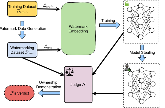
Figure 4: An overview of the watermarking process from watermark data generation to ownership demonstration.

5 Evaluation

We evaluate GENIE using 7 real-world datasets on 3 model architectures. We describe our experimental setup in §5.1. We evaluate the functionality preservation requirement of GENIE in §5.2. The robustness of GENIE is tested against 3 model extraction attacks (i.e., soft, hard, and double extraction; cf. §5.3.1) and 11 state-of-the-art backdoor defenses (i.e., 1 knowledge distillation (cf. §5.3.2), 4 model fine-tuning methods (cf. §5.3.3), 2 model compression techniques (cf. §5.3.4), 4 fine-pruning (cf. §5.3.5)). We further evaluate non-ownership piracy and efficiency requirements of GENIE in §5.4 and §5.5, respectively.

TABLE IV: Watermark verification performance (average of 10 runs) of GENIE across 3 model architectures and 7 datasets.

Dataset	SEAL			GCN			GraphSAGE
	$AUC_{\mathcal{D}_{test}}^{\mathcal{M}_{clean}}$ (%)	$AUC_{\mathcal{D}_{test}}^{\mathcal{M}_{wm}}$ (%)	$AUC_{\mathcal{D}_{wm}}^{\mathcal{M}_{wm}}$ (%)	$AUC_{\mathcal{D}_{test}}^{\mathcal{M}_{clean}}$ (%)	$AUC_{\mathcal{D}_{test}}^{\mathcal{M}_{wm}}$ (%)	$AUC_{\mathcal{D}_{wm}}^{\mathcal{M}_{wm}}$ (%)	$AUC_{\mathcal{D}_{test}}^{\mathcal{M}_{clean}}$ (%)	$AUC_{\mathcal{D}_{test}}^{\mathcal{M}_{wm}}$ (%)	$AUC_{\mathcal{D}_{wm}}^{\mathcal{M}_{wm}}$ (%)
C.ele	87.84 $\pm$ 0.46	87.60 $\pm$ 0.10	84.28 $\pm$ 0.93	88.97 $\pm$ 0.44	87.93 $\pm$ 0.43	100 $\pm$ 0.00	86.76 $\pm$ 0.68	85.71 $\pm$ 0.87	100 $\pm$ 0.00
USAir	93.19 $\pm$ 0.25	93.64 $\pm$ 0.17	92.29 $\pm$ 0.58	90.02 $\pm$ 0.52	89.35 $\pm$ 0.72	100 $\pm$ 0.00	92.44 $\pm$ 0.35	92.29 $\pm$ 0.65	100 $\pm$ 0.00
NS	98.10 $\pm$ 0.15	98.11 $\pm$ 0.23	98.70 $\pm$ 0.03	95.44 $\pm$ 0.74	96.26 $\pm$ 0.88	99.78 $\pm$ 0.00	90.90 $\pm$ 0.63	93.66 $\pm$ 0.47	99.78 $\pm$ 0.00
Yeast	97.07 $\pm$ 0.21	97.38 $\pm$ 0.16	97.69 $\pm$ 0.33	93.64 $\pm$ 0.40	91.73 $\pm$ 0.39	100 $\pm$ 0.00	89.12 $\pm$ 0.43	90.70 $\pm$ 0.43	100 $\pm$ 0.00
Power	84.41 $\pm$ 0.44	83.91 $\pm$ 0.25	88.28 $\pm$ 0.03	99.36 $\pm$ 0.17	99.12 $\pm$ 0.19	99.00 $\pm$ 0.00	87.54 $\pm$ 1.02	92.68 $\pm$ 1.06	99.00 $\pm$ 0.00
arXiv	98.14 $\pm$ 0.14	97.17 $\pm$ 0.49	98.15 $\pm$ 0.16	99.31 $\pm$ 0.04	98.78 $\pm$ 0.15	99.99 $\pm$ 0.00	99.62 $\pm$ 0.01	99.32 $\pm$ 0.13	99.99 $\pm$ 0.00
PPI	89.63 $\pm$ 0.12	89.45 $\pm$ 0.16	84.28 $\pm$ 1.38	95.08 $\pm$ 0.04	94.82 $\pm$ 0.05	100 $\pm$ 0.00	94.03 $\pm$ 0.09	94.31 $\pm$ 0.16	100 $\pm$ 0.00

5.1 Experimental setup

We run all our experiments on an NVIDIA DGX A100 machine using Pytorch [59] framework. In what follows, we describe the datasets, models, and metrics used in our work.

Datasets: Following prior works [25, 24], we use 7 publicly available real-world graph datasets of varying sizes and sparsities in our experiments. USAir [55] is a network of US Airlines with 332 nodes and 2,126 edges. NS [56] is a collaboration network of researchers in network science with 1,589 nodes and 2,742 edges. Yeast [52] is a protein-protein interaction network in yeast with 2,375 nodes and 11,693 edges. C.ele [54] is a neural network of C.elegans with 297 nodes and 2,148 edges. Power [54] is an electrical grid network of the western US with 4,941 nodes and 6,594 edges. arXiv [57] is a collaboration network of arXiv Astro Physics with 18,772 nodes and 198,110 edges from the popular Stanford SNAP dataset library. PPI [58] is a protein-protein interaction network with 3,890 nodes and 76,584 edges from BioGRID database.

It is worth highlighting that none of these datasets, except PPI, have node attributes. Since GENIE uses node attributes for watermark embedding, we generate node features using Node2Vec [24] for all the datasets. We follow 80-10-10 train-validation-test split of all the datasets across all our experiments. We use Adam optimizer and negative log likelihood loss for model training. Please refer Appendix A for our watermarking rates.

Models: We implement GENIE for SEAL [25] (in case of subgraph-based LP), and for GCN [8] as well as GraphSAGE [26] (in case of node representation-based LP).
SEAL: We use DGCNN as the GNN engine of SEAL. We use the default setting of DGCNN, i.e., four convolutional layers (32, 32, 32, 1 channels), a SortPooling layer (with $k=0.6$), two 1-D convolution layers (with 16, 32 output channels), and a 128-neuron dense layer. We train our models for a total of 50 epochs (for both training with or without a watermark).
GCN, SAGE: We use a 3-layer GCN and GraphSAGE models with a hidden layer of dimension 256. We use a 3-layer MLP for downstream binary classification with 256 hidden layer neurons. We train our models for a total of 400 epochs (for both training with or without a watermark).

Metric: We use AUC across all our experiments to evaluate the performance of GENIE. AUC is threshold independent and is a widely used metric for binary classification tasks, such as LP. AUC can be interpreted as the probability of a given classifier ranking a randomly chosen instance of a positive class higher than a randomly chosen instance of a negative class. Accordingly, a random classifier will have an AUC score of 0.5 [60].

We show the robustness of GENIE against various watermark-removal techniques in the following sections. $\mathcal{A}$ might fail or succeed while trying to remove watermark from $\mathcal{M}_{wm}$. We define the success and failure of GENIE as:
Success: If $AUC_{\mathcal{D}_{wm}}^{\mathcal{M}_{adv}}$ is above the watermark threshold after a watermark removal attempt, we identify it as a watermark success since we can verify the model’s ownership. If $AUC_{\mathcal{D}_{wm}}^{\mathcal{M}_{adv}}$ drops below the watermark threshold and $AUC_{\mathcal{D}_{test}}^{\mathcal{M}_{adv}}$ drops by more than 10%, we still consider it as a watermark success since $\mathcal{A}$ is losing the model’s utility in exchange of watermark removal attempt.
Failure: If $AUC_{\mathcal{D}_{wm}}^{\mathcal{M}_{adv}}$ drops below the watermark threshold and $AUC_{\mathcal{D}_{test}}^{\mathcal{M}_{adv}}$ doesn’t drop more than 10%, we consider it as a watermark failure since $\mathcal{A}$ was successful in removing the watermark without much loss of the model’s utility.

5.2 Functionality preserving

To evaluate the functionality-preserving nature of GENIE, we compare the performance of $\mathcal{M}_{clean}$ and $\mathcal{M}_{wm}$ on $\mathcal{D}_{test}$. We further assess the effectiveness of GENIE by evaluating the performance of $\mathcal{M}_{wm}$ on $\mathcal{D}_{wm}$. A high AUC score on $\mathcal{D}_{wm}$ indicates that the model has successfully learned to associate the watermark patterns with the predetermined incorrect predictions; enabling reliable watermark detection and ownership verification. TABLE IV presents $AUC_{\mathcal{D}_{test}}^{\mathcal{M}_{clean}}$, $AUC_{\mathcal{D}_{test}}^{\mathcal{M}_{wm}}$, $AUC_{\mathcal{D}_{wm}}^{\mathcal{M}_{wm}}$ across all 7 datasets and 3 model architectures considered in our work. The scores reported here are averaged from 10 runs using different random seeds (to mitigate potential seed influence and capture real the mean performance of GENIE). We observe that there is less than $2\%$ decrease in the AUC score on $\mathcal{D}_{test}$ due to watermarking across all model architectures for all datasets. These results allow us to claim that GENIE is functionality preserving. Since $AUC_{\mathcal{D}_{wm}}^{\mathcal{M}_{wm}}$ is more than $80\%$ across all model architectures for all datasets, we can claim that $\mathcal{M}_{wm}$ has successfully learned $\mathcal{F}_{wm}$. Interestingly, we observe an increase in AUC score on $\mathcal{D}_{test}$ after watermarking in a few cases, it could be a result of the watermarking embedding process acting as a regularizer, which reduces the overfitting nature of the model.

5.3 Robustness

To ensure the robustness and reliability of a watermarking scheme, it is crucial to assess its resilience against potential attempts by $\mathcal{A}$ to watermark. Since $\mathcal{A}$ cannot directly verify the presence of watermark in $\mathcal{M}_{wm}$, $\mathcal{A}$ may resort to various techniques (e.g., model extraction, model pruning, fine-tuning) to eliminate or degrade the embedded watermark. We conduct a series of evaluations to extensively examine the effectiveness of GENIE against a diverse set of robustness tests and potential attacks.

Due to the page length limit, here we present the results from robustness tests on GENIE for GCN only. We detail the corresponding results for SEAL and GraphSAGE in Appendix D.

5.3.1 Model extraction attacks

Such attacks [12, 13, 14] pose a significant threat to DNNs as they enable an adversary to steal the functionality of a victim model. In these attacks, $\mathcal{A}$ queries the victim model (i.e., $\mathcal{M}_{wm}$ in our case) using synthesized samples and collect responses to train a surrogate model (i.e., $\mathcal{M}_{adv}$) to steal $\mathcal{M}_{wm}$’s functionality. The literature on model extraction attacks is limited in the context of LP tasks on GNNs. Therefore, to evaluate GENIE against model extraction attacks, we modify the loss function employed in the knowledge distillation process [61] as outlined in Eq. 11 and Eq. 12.

$$\mathcal{L}_{soft}=\mathcal{L}_{CE}\left(\phi\left(\theta_{wm}\right),\phi\left(\theta_{adv}\right)\right).$$ (11)

$$\mathcal{L}_{hard}=\mathcal{L}_{CE}\left(\hat{y}\left(\theta_{wm}\right),\hat{y}\left(\theta_{adv}\right)\right).$$ (12)

Here, $\theta_{wm}$ and $\theta_{adv}$ denote the model parameters of $\mathcal{M}_{wm}$ and $\mathcal{M}_{adv}$, $\phi(\theta_{wm})$ and $\phi(\theta_{adv})$ represent the logits (i.e., output scores) produced by $\mathcal{M}_{wm}$ and $\mathcal{M}_{adv}$, while $\hat{y}(\theta_{wm})$ and $\hat{y}(\theta_{adv})$ denote the hard predictions (e.g., 0 or 1) made by the respective model. $\mathcal{L}_{CE}$ denotes cross-entropy loss.

We consider 3 types of model extraction techniques, viz., soft label, hard label, and double extraction. In soft label extraction, we apply $\mathcal{L}_{CE}$ between the logits of $\mathcal{M}_{wm}$ and $\mathcal{M}_{adv}$ to train $\mathcal{M}_{adv}$ (cf. Eq. 11). In hard label extraction, we apply $\mathcal{L}_{CE}$ between the predictions of $\mathcal{M}_{wm}$ and $\mathcal{M}_{adv}$ to train $\mathcal{M}_{adv}$ (cf. Eq. 12). In double extraction, we perform the hard label extraction twice to obtain the final $\mathcal{M}_{adv}$. Double extraction is a tougher setting since it is difficult for the watermark to survive model extraction twice. We train $\mathcal{M}_{adv}$ model using half of $\mathcal{D}_{test}$ and evaluate it with the other half. Table V shows $AUC_{\mathcal{D}_{test}}^{\mathcal{M}_{wm}}$, $AUC_{\mathcal{D}_{wm}}^{\mathcal{M}_{wm}}$ before model extraction and $AUC_{\mathcal{D}_{test}}^{\mathcal{M}_{adv}}$, $AUC_{\mathcal{D}_{wm}}^{\mathcal{M}_{adv}}$ after model extraction attack.

TABLE V: Impact of model extraction.

Dataset		C.ele	USAir	NS	Yeast	Power	arXiv	PPI
Before model extraction	$AUC_{\mathcal{D}_{test}}^{\mathcal{M}_{wm}}$ (%)	86.93	88.34	96.59	91.46	98.92	98.13	94.67
	$AUC_{\mathcal{D}_{wm}}^{\mathcal{M}_{wm}}$ (%)	100	100	99.77	100	99.00	100	100
After soft extraction	$AUC_{\mathcal{D}_{test}}^{\mathcal{M}_{adv}}$ (%)	87.35	89.00	95.74	91.57	98.21	98.28	94.93
	$AUC_{\mathcal{D}_{wm}}^{\mathcal{M}_{adv}}$ (%)	90.62	96.87	95.77	100	94.00	90.18	97.33
After hard extraction	$AUC_{\mathcal{D}_{test}}^{\mathcal{M}_{adv}}$ (%)	88.27	88.43	95.95	90.76	96.80	97.74	93.91
	$AUC_{\mathcal{D}_{wm}}^{\mathcal{M}_{adv}}$ (%)	82.81	90.91	94.88	100	90.99	82.35	87.14
After double extraction	$AUC_{\mathcal{D}_{test}}^{\mathcal{M}_{adv}}$ (%)	84.08	86.91	66.99	89.07	80.51	96.99	93.34
	$AUC_{\mathcal{D}_{wm}}^{\mathcal{M}_{adv}}$ (%)	65.62	78.32	65.55	92.30	77.00	43.43	53.85

We observe a maximum drop of 18.19% from $AUC_{\mathcal{D}_{wm}}^{\mathcal{M}_{wm}}$ to $AUC_{\mathcal{D}_{wm}}^{\mathcal{M}_{adv}}$ (for the C.ele dataset) under hard extraction attack, and a maximum drop of 9.82% (for the arXiv dataset) under soft extraction attack. Despite these drops, $AUC_{\mathcal{D}_{wm}}^{\mathcal{M}_{adv}}$ remains significantly above the watermark threshold (cf. TABLE III) in both cases, which ensures reliable ownership verification. We note a greater drop from $AUC_{\mathcal{D}_{wm}}^{\mathcal{M}_{wm}}$ to $AUC_{\mathcal{D}_{wm}}^{\mathcal{M}_{adv}}$ under hard extraction attack compared to soft extraction attack, which is naturally expected since logits provide richer information about the decision boundary than hard predictions. Despite a more significant drop from $AUC_{\mathcal{D}_{test}}^{\mathcal{M}_{wm}}$ to $AUC_{\mathcal{D}_{test}}^{\mathcal{M}_{adv}}$ and from $AUC_{\mathcal{D}_{wm}}^{\mathcal{M}_{wm}}$ to $AUC_{\mathcal{D}_{wm}}^{\mathcal{M}_{adv}}$ under double extraction attack, $AUC_{\mathcal{D}_{wm}}^{\mathcal{M}_{adv}}$ still remains substantially above the watermark threshold (cf. TABLE III) across all datasets. It demonstrates GENIE’s robustness against persistent model extraction attempts.

Different model architectures: It is also possible that $\mathcal{A}$ might not choose the same architecture to steal the model via model extraction. TABLE VI presents the outcomes of all 3 model extraction attacks when the $\mathcal{M}_{adv}$’s architecture (i.e., GraphSAGE) differs from $\mathcal{M}_{wm}$’s architecture (i.e., GCN). We find that $AUC_{\mathcal{D}_{wm}}^{\mathcal{M}_{adv}}$ is still above the watermark threshold (cf. TABLE III) under all attacks across all datasets; except for the power dataset under double extraction attack. However, $AUC_{\mathcal{D}_{test}}^{\mathcal{M}_{adv}}$ in that case drops from 98.93% to 58.81%, rendering the attack useless. Thus, we can conclude that GENIE is robust against model extraction attacks even when $\mathcal{M}_{adv}$ and $\mathcal{M}_{wm}$ have different architecture.

TABLE VI: Impact of model extraction when architecture of $\mathcal{M}_{adv}$ (i.e., GraphSAGE) differs from $\mathcal{M}_{wm}$ (i.e., GCN).

Dataset		C.ele	USAir	NS	Yeast	Power	arXiv	PPI
Before model extraction	$AUC_{\mathcal{D}_{test}}^{\mathcal{M}_{wm}}$ (%)	86.93	88.34	96.59	91.46	98.92	98.13	94.67
	$AUC_{\mathcal{D}_{wm}}^{\mathcal{M}_{wm}}$ (%)	100	100	99.77	100	99.00	100	100
After soft extraction	$AUC_{\mathcal{D}_{test}}^{\mathcal{M}_{adv}}$ (%)	87.14	88.89	78.52	90.42	70.51	98.29	94.61
	$AUC_{\mathcal{D}_{wm}}^{\mathcal{M}_{adv}}$ (%)	96.88	97.56	94.89	99.41	91.00	83.05	92.10
After hard extraction	$AUC_{\mathcal{D}_{test}}^{\mathcal{M}_{adv}}$ (%)	89.64	88.05	75.91	88.75	70.63	97.59	93.71
	$AUC_{\mathcal{D}_{wm}}^{\mathcal{M}_{adv}}$ (%)	93.75	95.31	98.00	89.94	91.00	71.93	83.65
After double extraction	$AUC_{\mathcal{D}_{test}}^{\mathcal{M}_{adv}}$ (%)	85.38	85.07	59.86	85.59	58.81	96.23	91.84
	$AUC_{\mathcal{D}_{wm}}^{\mathcal{M}_{adv}}$ (%)	79.69	78.71	66.67	67.46	49.50	41.90	47.75

5.3.2 Knowledge distillation

It is the process of transferring knowledge from a teacher model to a student model [61]. In our context, the teacher is $\mathcal{M}_{wm}$ and the student is $\mathcal{M}_{adv}$. The extraction process comprises training $\mathcal{M}_{adv}$ on the logits of $\mathcal{M}_{wm}$ and the ground truth [61]. It helps with decreasing the overfitting of the victim model (i.e., $\mathcal{M}_{wm}$). Consequently, $\mathcal{A}$ might be able to remove the watermark and reproduce the core model functionality.

To test GENIE’s robustness, we assume that the student model have the same architecture as the teacher model. Moreover, we use half of $\mathcal{D}_{test}$ for distillation and evaluate $\mathcal{M}_{adv}$ on the other half. TABLE VII presents $AUC_{\mathcal{D}_{test}}^{\mathcal{M}_{wm}}$, $AUC_{\mathcal{D}_{wm}}^{\mathcal{M}_{wm}}$ before knowledge distillation and $AUC_{\mathcal{D}_{test}}^{\mathcal{M}_{adv}}$, $AUC_{\mathcal{D}_{wm}}^{\mathcal{M}_{adv}}$ after knowledge distillation.

TABLE VII: Impact of knowledge distillation.

Dataset		C.ele	USAir	NS	Yeast	Power	arXiv	PPI
Before distillation	$AUC_{\mathcal{D}_{test}}^{\mathcal{M}_{wm}}$ (%)	86.93	88.34	96.59	91.46	98.92	98.13	94.67
	$AUC_{\mathcal{D}_{wm}}^{\mathcal{M}_{wm}}$ (%)	100	100	99.77	100	99.00	100	100
After distillation	$AUC_{\mathcal{D}_{test}}^{\mathcal{M}_{adv}}$ (%)	88.60	89.39	95.00	92.19	98.54	98.71	95.25
	$AUC_{\mathcal{D}_{wm}}^{\mathcal{M}_{adv}}$ (%)	81.25	86.33	90.89	98.22	86.00	74.76	94.95

We observe a maximum drop of 25.24% from $AUC_{\mathcal{D}_{wm}}^{\mathcal{M}_{wm}}$ to $AUC_{\mathcal{D}_{wm}}^{\mathcal{M}_{adv}}$ (for the arXiv dataset). It important to note that $AUC_{\mathcal{D}_{wm}}^{\mathcal{M}_{adv}}$ still remains significantly above the watermark threshold (cf. TABLE III), which indicates that $\mathcal{A}$ was not successful in removing the watermark using knowledge distillation. To summarize, our results show that knowledge distillation was able to transfer the core functionality of the victim model, but the watermark was transferred too (as $AUC_{\mathcal{D}_{wm}}^{\mathcal{M}_{adv}}$ is still above the threshold for all datasets). We can conclude that GENIE is robust against knowledge distillation.

5.3.3 Model fine-tuning

Fine-tuning [62] is one of the most commonly used attacks to remove the watermark since it is computationally inexpensive and does not compromise the model’s core functionality much. To test GENIE against this attack, we use half of $\mathcal{D}_{test}$ for fine-tuning and evaluate the fine-tuned model’s (i.e., $\mathcal{M}_{adv}$) performance with the other half. Through extensive experimentation and analysis, we determined that limiting the training process to 50 epochs serves as an optimal strategy (i.e., to avoid the risk of overfitting $\mathcal{M}_{adv}$ on the subset of $\mathcal{D}_{test}$ used for fine-tuning). We evaluate GENIE against 4 variations of fine-tuning. These can be classified into two broad categories [62]:

Last layer fine-tuning: This fine-tuning procedure updates the weights of only the last layer of the target model. It can be done in the following two ways.

1. Fine-Tune Last Layer (FTLL): Freezing the weights of the target model, updating the weights of its last layer only during fine-tuning.

2. Re-Train Last Layer (RTLL): Freezing the weights of the target model, reinitializing the weights of only its last layer, and then fine-tuning it.

All layers fine-tuning: This fine-tuning procedure updates weights of all the layers of the target model. It is a stronger setting compared to the last layer fine-tuning method as all the weights are updated, which makes it tougher to retain the watermark. It can be done in the following two ways.

1. Fine-Tune All Layers (FTAL): Updating weights of all the layers of the target model during fine-tuning.

2. Re-Train All Layers (RTAL): Reinitializing the weights of target model’s last layer, updating weights of all its layers during fine-tuning.

FTLL is considered the weakest attack because it has the least capacity to modify the core GNN layers responsible for learning the watermark. Conversely, RTAL is considered the toughest attack because it enables complete fine-tuning of all model layers, providing the highest flexibility to potentially overwrite or distort the watermark embedded across multiple layers. TABLE VIII lists $AUC_{\mathcal{D}_{test}}^{\mathcal{M}_{wm}}$, $AUC_{\mathcal{D}_{wm}}^{\mathcal{M}_{wm}}$ before fine-tuning (in column with $\star$) and $AUC_{\mathcal{D}_{test}}^{\mathcal{M}_{adv}}$, $AUC_{\mathcal{D}_{wm}}^{\mathcal{M}_{adv}}$ after fine-tuning with all the four types.

TABLE VIII: Impact of model fine-tuning.

Dataset		Fine-tuning method
		$\text{No fine-tuning}^{\star}$	FTLL	RTLL	FTAL	RTAL
C.ele	$AUC_{\mathcal{D}_{test}}^{\mathcal{M}_{adv}}$ (%)	86.93	82.46	70.61	74.79	68.51
	$AUC_{\mathcal{D}_{wm}}^{\mathcal{M}_{adv}}$ (%)	100	90.62	60.94	73.44	53.12
USAir	$AUC_{\mathcal{D}_{test}}^{\mathcal{M}_{adv}}$ (%)	88.34	89.09	87.68	86.79	84.68
	$AUC_{\mathcal{D}_{wm}}^{\mathcal{M}_{adv}}$ (%)	100	90.62	81.64	80.52	69.24
NS	$AUC_{\mathcal{D}_{test}}^{\mathcal{M}_{adv}}$ (%)	96.59	98.70	98.59	89.99	73.95
	$AUC_{\mathcal{D}_{wm}}^{\mathcal{M}_{adv}}$ (%)	99.77	99.78	96.22	93.56	71.78
Yeast	$AUC_{\mathcal{D}_{test}}^{\mathcal{M}_{adv}}$ (%)	91.46	91.61	90.79	90.33	87.08
	$AUC_{\mathcal{D}_{wm}}^{\mathcal{M}_{adv}}$ (%)	100	91.72	89.35	98.22	63.91
Power	$AUC_{\mathcal{D}_{test}}^{\mathcal{M}_{adv}}$ (%)	98.92	99.39	99.26	97.74	95.05
	$AUC_{\mathcal{D}_{wm}}^{\mathcal{M}_{adv}}$ (%)	99.00	99.00	99.00	77.00	73.00
arXiv	$AUC_{\mathcal{D}_{test}}^{\mathcal{M}_{adv}}$ (%)	98.13	98.57	97.65	98.78	98.04
	$AUC_{\mathcal{D}_{wm}}^{\mathcal{M}_{adv}}$ (%)	100	88.23	46.54	55.54	19.92
PPI	$AUC_{\mathcal{D}_{test}}^{\mathcal{M}_{adv}}$ (%)	94.67	94.94	94.35	94.94	94.35
	$AUC_{\mathcal{D}_{wm}}^{\mathcal{M}_{adv}}$ (%)	100	94.95	55.46	77.96	48.67
Column with ⋆ shows the values when $\mathcal{M}_{adv}$ = $\mathcal{M}_{wm}$.

We note that our watermark survives against all fine-tuning procedures for all the datasets; since $AUC_{\mathcal{D}_{wm}}^{\mathcal{M}_{adv}}$ remains above the watermark threshold (cf. TABLE III) in each case. Therefore, we conclude that GENIE is robust against model fine-tuning.

5.3.4 Model compression

It is a technique to reduce the size and complexity of a DNN, thereby making it more efficient and easily deployable. Compressing the model can inadvertently or otherwise act as an attack against the watermark. Thus, we test GENIE’s robustness with following two model compression techniques:

Model pruning: Model or parameter pruning [63] selects a fraction of weights that have the smallest absolute value and makes them zero. It is a computationally inexpensive backdoor defense. We evaluate GENIE against different pruning fractions starting from 0.2 at a step size of 0.2. TABLE IX lists $AUC_{\mathcal{D}_{test}}^{\mathcal{M}_{wm}}$, $AUC_{\mathcal{D}_{wm}}^{\mathcal{M}_{wm}}$ before model pruning (in column with $\star$) and $AUC_{\mathcal{D}_{test}}^{\mathcal{M}_{adv}}$, $AUC_{\mathcal{D}_{wm}}^{\mathcal{M}_{adv}}$ after model pruning with different prune percentage. We see that even after pruning 80% of $\mathcal{M}_{wm}$’s weights, we are still able to verify the ownership from the resultant $\mathcal{M}_{adv}$ in almost every case. Given that $AUC_{\mathcal{D}_{wm}}^{\mathcal{M}_{adv}}$ remains above the watermark threshold (cf. TABLE III) roughly in all cases, we conclude that GENIE is robust against model pruning.

TABLE IX: Impact of model pruning.

Dataset		Prune Percentage (%)
		$\text{No Pruning}^{\star}$	20	40	60	80	100
C.ele	$AUC_{\mathcal{D}_{test}}^{\mathcal{M}_{adv}}$ (%)	86.93	86.97	86.31	83.92	75.43	50.00
	$AUC_{\mathcal{D}_{wm}}^{\mathcal{M}_{adv}}$ (%)	100	100	100	100	70.31	50.00
USAir	$AUC_{\mathcal{D}_{test}}^{\mathcal{M}_{adv}}$ (%)	88.34	88.98	89.57	89.21	78.50	50.00
	$AUC_{\mathcal{D}_{wm}}^{\mathcal{M}_{adv}}$ (%)	100	100	100	92.77	71.28	50.00
NS	$AUC_{\mathcal{D}_{test}}^{\mathcal{M}_{adv}}$ (%)	96.59	96.25	96.01	96.08	91.31	50.00
	$AUC_{\mathcal{D}_{wm}}^{\mathcal{M}_{adv}}$ (%)	99.77	99.77	99.77	96.66	85.55	50.00
Yeast	$AUC_{\mathcal{D}_{test}}^{\mathcal{M}_{adv}}$ (%)	91.46	91.27	89.97	85.71	80.50	50.00
	$AUC_{\mathcal{D}_{wm}}^{\mathcal{M}_{adv}}$ (%)	100	100	100	100	74.55	50.00
Power	$AUC_{\mathcal{D}_{test}}^{\mathcal{M}_{adv}}$ (%)	98.92	99.00	99.20	98.32	92.43	50.00
	$AUC_{\mathcal{D}_{wm}}^{\mathcal{M}_{adv}}$ (%)	99.00	99.00	95.00	74.00	55.00	50.00
arXiv	$AUC_{\mathcal{D}_{test}}^{\mathcal{M}_{adv}}$ (%)	98.13	98.08	97.911	94.79	84.37	50.00
	$AUC_{\mathcal{D}_{wm}}^{\mathcal{M}_{adv}}$ (%)	100	100	99.98	83.09	41.95	50.00
PPI	$AUC_{\mathcal{D}_{test}}^{\mathcal{M}_{adv}}$ (%)	94.67	94.60	94.05	92.86	90.06	50.00
	$AUC_{\mathcal{D}_{wm}}^{\mathcal{M}_{adv}}$ (%)	100	100	100	78.87	31.22	50.00
Column with ⋆ shows the values when $\mathcal{M}_{adv}$ = $\mathcal{M}_{wm}$.

Weight quantization: It is another model compression technique to reduce the size of a model. It changes the representation of weights to a lower-bit system, thereby saving memory. It is often used to compress large models, e.g., LLMs [64]. We follow the standard weight quantization method [65] with bit-size $=3$. TABLE X reports that $AUC_{\mathcal{D}_{wm}}^{\mathcal{M}_{adv}}$ remains remarkably above the watermark threshold (cf. TABLE III) after quantization in all the cases, making GENIE is robust against weight quantization.

TABLE X: Impact of weight quantization.

Dataset		C.ele	USAir	NS	Yeast	Power	arXiv	PPI
Before quantization	$AUC_{\mathcal{D}_{test}}^{\mathcal{M}_{wm}}$ (%)	86.93	88.34	96.59	91.46	98.92	98.13	94.67
	$AUC_{\mathcal{D}_{wm}}^{\mathcal{M}_{wm}}$ (%)	100	100	99.77	100	99.00	100	100
After quantization	$AUC_{\mathcal{D}_{test}}^{\mathcal{M}_{adv}}$ (%)	84.59	85.16	97.79	85.84	98.39	96.07	87.56
	$AUC_{\mathcal{D}_{wm}}^{\mathcal{M}_{adv}}$ (%)	96.88	90.92	99.78	82.25	98.00	81.58	67.95

5.3.5 Fine-pruning

It is a key defense against a backdoor attack that combines model pruning and fine-tuning. It is more effective than individual pruning or fine-tuning, which makes it difficult for the watermark to survive. We start by pruning a fraction of the smallest absolute weights. Next, we fine-tune the pruned model with half of $\mathcal{D}_{test}$ and evaluate the pruned+fine-tuned model (i.e., $\mathcal{M}_{adv}$) with the other half. We perform an exhaustive evaluation with pruning fractions ranging from 0.2-0.8 at a step size of 0.2, which is followed by one of the four types of model fine-tuning (i.e., FTLL, RTLL, FTAL, RTAL). Our rigorous experiments aim to provide a holistic understanding of GENIE’s robustness against the fine-pruning technique. TABLEs XI-XIV exhibit $AUC_{\mathcal{D}_{test}}^{\mathcal{M}_{wm}}$, $AUC_{\mathcal{D}_{wm}}^{\mathcal{M}_{wm}}$ before fine-pruning (in column with $\star$) and $AUC_{\mathcal{D}_{test}}^{\mathcal{M}_{adv}}$, $AUC_{\mathcal{D}_{wm}}^{\mathcal{M}_{adv}}$ after fine-pruning with different pruning fractions and fine-tuning methods.

TABLE XI: Impact of pruning + FTLL.

Dataset		Prune Percentage (%)
		$\text{No Pruning}^{\star}$	20	40	60	80
C.ele	$AUC_{\mathcal{D}_{test}}^{\mathcal{M}_{adv}}$ (%)	86.93	82.01	80.80	78.54	82.57
	$AUC_{\mathcal{D}_{wm}}^{\mathcal{M}_{adv}}$ (%)	100	93.75	90.62	81.25	79.68
USAir	$AUC_{\mathcal{D}_{test}}^{\mathcal{M}_{adv}}$ (%)	88.34	89.15	88.85	88.30	87.93
	$AUC_{\mathcal{D}_{wm}}^{\mathcal{M}_{adv}}$ (%)	100	91.21	90.42	87.50	69.82
NS	$AUC_{\mathcal{D}_{test}}^{\mathcal{M}_{adv}}$ (%)	96.59	98.49	98.22	97.55	97.26
	$AUC_{\mathcal{D}_{wm}}^{\mathcal{M}_{adv}}$ (%)	99.77	99.77	98.88	97.55	93.11
Yeast	$AUC_{\mathcal{D}_{test}}^{\mathcal{M}_{adv}}$ (%)	91.46	91.52	91.41	89.90	86.64
	$AUC_{\mathcal{D}_{wm}}^{\mathcal{M}_{adv}}$ (%)	100	91.71	90.53	85.20	92.30
Power	$AUC_{\mathcal{D}_{test}}^{\mathcal{M}_{adv}}$ (%)	98.92	99.38	99.30	98.91	98.04
	$AUC_{\mathcal{D}_{wm}}^{\mathcal{M}_{adv}}$ (%)	99.00	99.00	95.00	87.00	72.00
arXiv	$AUC_{\mathcal{D}_{test}}^{\mathcal{M}_{adv}}$ (%)	98.13	98.54	98.41	98.07	96.74
	$AUC_{\mathcal{D}_{wm}}^{\mathcal{M}_{adv}}$ (%)	100	86.51	81.81	59.24	30.07
PPI	$AUC_{\mathcal{D}_{test}}^{\mathcal{M}_{adv}}$ (%)	94.67	94.92	94.73	94.63	93.41
	$AUC_{\mathcal{D}_{wm}}^{\mathcal{M}_{adv}}$ (%)	100	96.32	88.52	79.43	51.97
Column with ⋆ shows the values when $\mathcal{M}_{adv}$ = $\mathcal{M}_{wm}$.

TABLE XII: Impact of pruning + RTLL.

Dataset		Prune Percentage (%)
		$\text{No Pruning}^{\star}$	20	40	60	80
C.ele	$AUC_{\mathcal{D}_{test}}^{\mathcal{M}_{adv}}$ (%)	86.93	70.65	71.04	73.56	79.64
	$AUC_{\mathcal{D}_{wm}}^{\mathcal{M}_{adv}}$ (%)	100	59.37	57.81	68.75	84.37
USAir	$AUC_{\mathcal{D}_{test}}^{\mathcal{M}_{adv}}$ (%)	88.34	87.57	87.50	88.09	86.59
	$AUC_{\mathcal{D}_{wm}}^{\mathcal{M}_{adv}}$ (%)	100	82.12	82.81	79.58	61.62
NS	$AUC_{\mathcal{D}_{test}}^{\mathcal{M}_{adv}}$ (%)	96.59	98.43	98.18	97.74	96.72
	$AUC_{\mathcal{D}_{wm}}^{\mathcal{M}_{adv}}$ (%)	99.77	96.66	97.55	96.22	94.44
Yeast	$AUC_{\mathcal{D}_{test}}^{\mathcal{M}_{adv}}$ (%)	91.46	90.72	90.19	88.87	86.24
	$AUC_{\mathcal{D}_{wm}}^{\mathcal{M}_{adv}}$ (%)	100	88.16	88.16	77.51	84.61
Power	$AUC_{\mathcal{D}_{test}}^{\mathcal{M}_{adv}}$ (%)	98.92	99.24	99.16	98.73	97.40
	$AUC_{\mathcal{D}_{wm}}^{\mathcal{M}_{adv}}$ (%)	99.00	99.00	93.00	91.99	71.00
arXiv	$AUC_{\mathcal{D}_{test}}^{\mathcal{M}_{adv}}$ (%)	98.13	98.54	98.41	98.07	96.74
	$AUC_{\mathcal{D}_{wm}}^{\mathcal{M}_{adv}}$ (%)	100	44.95	47.04	48.31	39.69
PPI	$AUC_{\mathcal{D}_{test}}^{\mathcal{M}_{adv}}$ (%)	94.67	94.21	94.04	93.54	92.78
	$AUC_{\mathcal{D}_{wm}}^{\mathcal{M}_{adv}}$ (%)	100	59.41	51.42	53.16	46.28
Column with ⋆ shows the values when $\mathcal{M}_{adv}$ = $\mathcal{M}_{wm}$.

We observe the highest drop from $AUC_{\mathcal{D}_{wm}}^{\mathcal{M}_{wm}}$ to $AUC_{\mathcal{D}_{wm}}^{\mathcal{M}_{adv}}$ when fine-pruning is performed using RTAL (cf. TABLE XIV), which is expected as RTAL represents the strongest attack that enables complete fine-tuning of all model layers. Nevertheless, $AUC_{\mathcal{D}_{wm}}^{\mathcal{M}_{adv}}$ remains above the watermark threshold (cf. TABLE III) in most cases. We strongly believe that GENIE is robust against fine-pruning given that it is failing at only 2 out of 112 cases.

TABLE XIII: Impact of pruning + FTAL.

Dataset		Prune Percentage (%)
		$\text{No Pruning}^{\star}$	20	40	60	80
C.ele	$AUC_{\mathcal{D}_{test}}^{\mathcal{M}_{adv}}$ (%)	86.93	75.73	77.27	75.46	74.68
	$AUC_{\mathcal{D}_{wm}}^{\mathcal{M}_{adv}}$ (%)	100	71.87	60.93	78.12	62.50
USAir	$AUC_{\mathcal{D}_{test}}^{\mathcal{M}_{adv}}$ (%)	88.34	86.35	85.96	86.94	85.23
	$AUC_{\mathcal{D}_{wm}}^{\mathcal{M}_{adv}}$ (%)	100	81.49	73.19	76.31	63.28
NS	$AUC_{\mathcal{D}_{test}}^{\mathcal{M}_{adv}}$ (%)	96.59	91.90	89.33	88.09	87.84
	$AUC_{\mathcal{D}_{wm}}^{\mathcal{M}_{adv}}$ (%)	99.77	89.11	84.66	88.66	92.22
Yeast	$AUC_{\mathcal{D}_{test}}^{\mathcal{M}_{adv}}$ (%)	91.46	90.48	90.06	89.43	87.45
	$AUC_{\mathcal{D}_{wm}}^{\mathcal{M}_{adv}}$ (%)	100	100	100	99.40	81.65
Power	$AUC_{\mathcal{D}_{test}}^{\mathcal{M}_{adv}}$ (%)	98.92	97.36	97.39	97.69	96.97
	$AUC_{\mathcal{D}_{wm}}^{\mathcal{M}_{adv}}$ (%)	99.00	88.00	87.00	84.00	67.99
arXiv	$AUC_{\mathcal{D}_{test}}^{\mathcal{M}_{adv}}$ (%)	98.13	98.78	98.79	98.80	98.48
	$AUC_{\mathcal{D}_{wm}}^{\mathcal{M}_{adv}}$ (%)	100	54.45	48.18	33.05	17.00
PPI	$AUC_{\mathcal{D}_{test}}^{\mathcal{M}_{adv}}$ (%)	94.67	94.02	94.04	93.93	93.87
	$AUC_{\mathcal{D}_{wm}}^{\mathcal{M}_{adv}}$ (%)	100	78.60	75.39	66.20	45.36
Column with ⋆ shows the values when $\mathcal{M}_{adv}$ = $\mathcal{M}_{wm}$.

TABLE XIV: Impact of pruning + RTAL.

Dataset		Prune Percentage (%)
		$\text{No Pruning}^{\star}$	20	40	60	80
C.ele	$AUC_{\mathcal{D}_{test}}^{\mathcal{M}_{adv}}$ (%)	86.93	69.11	66.34	72.06	68.28
	$AUC_{\mathcal{D}_{wm}}^{\mathcal{M}_{adv}}$ (%)	100	68.75	68.75	70.31	75.00
USAir	$AUC_{\mathcal{D}_{test}}^{\mathcal{M}_{adv}}$ (%)	88.34	85.46	84.94	83.26	84.50
	$AUC_{\mathcal{D}_{wm}}^{\mathcal{M}_{adv}}$ (%)	100	63.76	65.52	62.79	47.75
NS	$AUC_{\mathcal{D}_{test}}^{\mathcal{M}_{adv}}$ (%)	96.59	76.49	79.69	74.29	74.74
	$AUC_{\mathcal{D}_{wm}}^{\mathcal{M}_{adv}}$ (%)	99.77	78.00	85.11	78.88	78.88
Yeast	$AUC_{\mathcal{D}_{test}}^{\mathcal{M}_{adv}}$ (%)	91.46	85.70	85.47	84.50	82.89
	$AUC_{\mathcal{D}_{wm}}^{\mathcal{M}_{adv}}$ (%)	100	84.02	92.89	89.94	63.31
Power	$AUC_{\mathcal{D}_{test}}^{\mathcal{M}_{adv}}$ (%)	98.92	92.87	92.33	91.92	90.02
	$AUC_{\mathcal{D}_{wm}}^{\mathcal{M}_{adv}}$ (%)	99.00	63.00	64.99	63.00	49.99
arXiv	$AUC_{\mathcal{D}_{test}}^{\mathcal{M}_{adv}}$ (%)	98.13	98.02	98.01	97.61	95.82
	$AUC_{\mathcal{D}_{wm}}^{\mathcal{M}_{adv}}$ (%)	100	20.67	19.46	17.99	13.93
PPI	$AUC_{\mathcal{D}_{test}}^{\mathcal{M}_{adv}}$ (%)	94.67	92.92	92.79	92.45	91.88
	$AUC_{\mathcal{D}_{wm}}^{\mathcal{M}_{adv}}$ (%)	100	42.51	44.81	46.74	27.08
Column with ⋆ shows the values when $\mathcal{M}_{adv}$ = $\mathcal{M}_{wm}$.

5.4 Non-ownership piracy

$\mathcal{A}$ may attempt to follow GENIE to insert his pirated watermark into a model stolen from $\mathcal{O}$ (i.e., $\mathcal{M}_{wm}$). However, owing to the robustness of GENIE (as witnessed in § 5.3), $\mathcal{A}$ will not be able to remove $\mathcal{O}$’s original watermark from $\mathcal{M}_{wm}$. Consequently, $\mathcal{A}$ cannot derive $\mathcal{M}_{adv}$ from $\mathcal{M}_{wm}$, which solely contains his pirated watermark and not $\mathcal{O}$’s original watermark.

GENIE injects watermark into an untrained model while $\mathcal{A}$ has access to only $\mathcal{M}_{wm}$. In a real-world setting, $\mathcal{A}$ can still generate his own pirated trigger set (using the method explained in § 4.1) and train stolen $\mathcal{M}_{wm}$ on the pirated trigger set to obtain $\mathcal{M}_{adv}$ (generally called a pirated model). Given that training on just the pirated trigger set might lead to decrease in $AUC_{\mathcal{D}_{test}}^{\mathcal{M}_{adv}}$, $\mathcal{A}$ would want to identify an optimal number of epochs for training with the pirated trigger set such that $\mathcal{M}_{adv}$ has high AUC on both $\mathcal{D}_{test}$ and the pirated trigger set. Figure 5 shows the variations in $\mathcal{M}_{adv}$’s performance on $\mathcal{D}_{wm}$, $\mathcal{D}_{test}$, and pirated trigger set during pirated watermark embedding process across different numbers of epochs for GCN over NS dataset; cf. Appendix D.3 for other datasets.

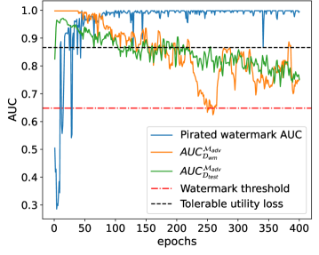
Figure 5: A representative example of $\mathcal{M}_{adv}$’s performance trajectory on $\mathcal{D}_{wm}$, $\mathcal{D}_{test}$, and pirated trigger set during embedding of pirated watermark across training epochs.

We see that $\mathcal{M}_{adv}$ performs well on $\mathcal{D}_{wm}$, $\mathcal{D}_{test}$, as well as on pirated trigger sets around $20^{th}$ epoch. If $\mathcal{O}$ challenges $\mathcal{A}$ to present his model at this point, $\mathcal{M}_{adv}$ will contain $\mathcal{A}$’s pirated watermark as well as $\mathcal{O}$’s watermark. However, $\mathcal{O}$ can present $\mathcal{M}_{wm}$ containing only her watermark. Thus, identifying the true owner will be easy in such a dispute. We further observe that around $250^{th}$ epoch, $AUC_{\mathcal{D}_{wm}}^{\mathcal{M}_{adv}}$ drops below the watermark threshold (cf. TABLE III), but $AUC_{\mathcal{D}_{test}}^{\mathcal{M}_{adv}}$ falls below the tolerable utility loss (i.e., up to 10%; following the definition of failure in §5.1) $\mathcal{A}$ is willing to tolerate. Even if $\mathcal{A}$ chooses to train for even higher epochs while embedding the pirated watermark, $\mathcal{M}_{adv}$ continues to lose its utility; rendering the $\mathcal{M}_{adv}$ useless. Hence, we take the liberty to claim that GENIE is robust against piracy attacks (i.e., $\mathcal{A}$ cannot fraudulently claim ownership or fabricate watermark over a pirated model).

5.5 Efficiency

The computational efficiency of a watermarking scheme is a critical aspect since it directly affects its cost and practical adoption. We rigorously evaluate the efficiency of GENIE by comparing the time required for the standard model training with the time needed for watermark embedding (which includes the time dedicated to generate $\mathcal{D}_{wm}$). In practice, the overall computational overhead mainly depends on the percentage of samples we choose to create $\mathcal{D}_{wm}$. If the $\mathcal{D}_{wm}$ is too big, embedding watermark information might take longer and even lead to a considerable loss in utility. On the other side, if $\mathcal{D}_{wm}$ is too small, it would be easier for $\mathcal{A}$ to remove the watermark (for instance, via pruning, fine-tuning).

We empirically observed that using percentage of samples up to 40% is optimal for SEAL, GCN, and GraphSAGE. It is the same percentage of samples we used in all our evaluations. TABLE XV shows the time needed for the standard model training against the time required for GENIE’s watermark embedding. Our results indicate that GENIE has reasonable computational overhead in exchange of the invaluable IP protection it confers to a model. SEAL over Yeast dataset consumed the maximum additional training time, which is only 18.3% more than the standard training time. Therefore, we argue that GENIE is efficient.

TABLE XV: Standard vs. watermark training in seconds.

Dataset	SEAL		GCN		GraphSAGE
	$T_{std}$	$T_{wm}$	$T_{std}$	$T_{wm}$	$T_{std}$	$T_{wm}$
C.ele	197.073	294.520	8.723	11.969	9.740	13.650
USAir	197.822	261.690	8.464	11.940	9.357	13.694
NS	112.798	138.869	8.933	12.365	9.909	14.224
Yeast	576.529	682.085	13.146	15.704	14.008	17.634
Power	270.702	345.792	11.229	14.283	12.130	16.612
arXiv	2009.926	2072.909	64.396	70.534	67.059	75.979
PPI	1048.213	1108.650	23.485	24.500	24.648	26.136

6 Discussion, limitation, future work

Our thorough evaluations show that GENIE satisfies all the watermarking requirements (cf. §3), i.e., functionality preservation (cf. §5.2), Un-removability (cf. §5.3), non-ownership piracy (cf. §5.4), efficiency (cf. §5.5), non-trivial ownership (cf. §4.3), capacity requirement does not apply to it since GENIE is a zero-bit watermarking scheme, and we evaluated GENIE on 3 GNN model architectures and 7 real-world datasets for the generality requirement. Given the salient features of GENIE, especially its efficiency in accommodating large datasets and performance on diverse datasets of varying scales and sparsities, we can claim that GENIE is suitable for real-world applications.

Uniqueness: As discussed in §2.4, the two state-of-the-art backdoor attacks on LP [42, 43] are not practical for watermarking LP task in GNNs. To this end, we implement GENIE using a backdoor that employs watermark feature vector (as described in §4.1.1 and §4.1.2) for watermarking GNNs without Data Poisoning (i.e., merging $\mathcal{D}_{wm}$ to $\mathcal{D}_{train}$ at each epoch) [37]. As opposed to the conventional data poisoning-based backdoor attacks [16], where loss function remains untouched, we propose two different loss functions (viz., $\mathcal{L}_{train}$, $\mathcal{L}_{wm}$) and a unique method of optimizing them individually. In particular, we use the gradient update mechanism described in Eq. 8 for the loss function optimization. Our unique improvements cater to the superior performance of our proposed watermark injection method.

Stealthiness: A crucial requirement for a watermarking scheme is its evasiveness to detection. §5.2 demonstrates that $\mathcal{M}_{clean}$ and $\mathcal{M}_{wm}$ are indistinguishable in terms of their behavior on $\mathcal{D}_{test}$, proving the stealthiness of GENIE. The behavior of these models differs only on $\mathcal{D}_{wm}$. It is worth highlighting that only $\mathcal{O}$ has access to $\mathcal{D}_{wm}$ while it is computationally infeasible for $\mathcal{A}$ to guess the trigger set.

Limitation: Despite extensive empirical evaluations of GENIE in our study, GENIE does not currently have the theoretical guarantees required to ensure that the watermark will not be removed by any new attack in the future. Nevertheless, we present a competitive ownership demonstration scheme that statistically guarantees FPR and FNR of GENIE to be less than $10^{-6}$.

Future work: We will evaluate GENIE with more GNN architectures to further ensure its generalizability. In this paper, we consider LP in a transductive setting, which is considered as the default setting for LP task. In the future, we will extend GENIE to an inductive setting. Finally, all the graphs considered in this work are static. In the future, we will explore the applicability of GENIE to dynamic graphs.

7 Conclusion

Despite the tremendous success of GNNs in learning graph-structured data, protecting trained GNN models from model-stealing attacks is a critical issue. Existing GNN watermarking schemes focus either on node or graph classification tasks. In this paper, we propose GENIE, a backdoor-based watermarking scheme for GNNs tailored to LP task. We design GENIE for node representation-based and subgraph-based methods of LP. Our extensive evaluations show that GENIE is functionality-preserving. At the same time, GENIE is robust against state-of-the-art backdoor defenses and model extraction attacks. The statistical guarantees given by the ownership demonstration process confirm a close to zero probability of misclassification in GENIE. We hope our work sets new research directions and benchmarks in the domain of model watermarking.

Appendix A provides further details on our experiment setup. Appendix B elucidates the statistical guarantee of the non-trivial ownership requirement of watermarking in GENIE. Appendix C explains our watermark threshold calculations. Appendix D lists additional results for GENIE on GraphSAGE, SEAL, and GCN. Appendix E presents GENIE’s performance on three additional datasets.

Appendix A Further details on our experiment setup

We use a learning rate of 0.0001 for SEAL and 0.001 for GCN and GraphSAGE. Both $\mathcal{L}_{train}$ and $\mathcal{L}_{wm}$ use the same loss function (i.e., negative log likelihood) and optimizer (i.e., Adam) with the same learning rate. TABLE A.1 lists our watermarking rate for each dataset and respective model.

TABLE A.1: Watermarking rate (%) used in our experiments.

Dataset	C.ele	USAir	NS	Yeast	Power	arXiv	PPI
GCN	10	15	10	4	5	4	4
GraphSAGE	10	15	10	4	5	3	4
SEAL	30	30	35	20	40	-	-

Appendix B Statistical guarantee of non-trivial ownership in GENIE

The values of $AUC_{\mathcal{D}_{wm}}^{\mathcal{M}_{clean}}$ and $AUC_{\mathcal{D}_{wm}}^{\mathcal{M}_{wm}}$ are given for $n=10$ different $\mathcal{M}_{clean}$ and ($\mathcal{D}_{wm}$, $\mathcal{M}_{wm}$) in TABLE B.1 (for SEAL), TABLE B.2 (for GCN), and TABLE B.3 (for GraphSAGE). The corresponding $p$-values are also mentioned. For each dataset and architecture, the $p$-value is observed to be below the significance level, i.e., $1-\tau=0.05$. Therefore, we reject $\mathbf{H}_{0}$ for each architecture and dataset as described in §4.3.

TABLE B.1: Non-trivial ownership results for SEAL.

Dataset	Model ($\mathcal{M}$)	$AUC_{\mathcal{D}_{wm}}^{\mathcal{M}}$ (%)										$p$-value
C.ele	$\mathcal{M}_{clean}$	38.63	25.60	23.70	28.72	22.48	23.29	20.39	22.62	26.83	24.97	0.000
	$\mathcal{M}_{wm}$	76.58	77.19	77.32	78.91	78.72	77.69	78.24	77.39	78.24	75.94
USAir	$\mathcal{M}_{clean}$	8.00	6.97	5.88	7.10	7.61	7.92	6.92	8.72	7.72	8.79	0.000
	$\mathcal{M}_{wm}$	94.01	94.02	94.65	93.59	93.81	95.17	95.39	94.13	94.08	94.14
NS	$\mathcal{M}_{clean}$	3.41	1.73	2.25	2.57	1.91	1.72	2.04	2.50	3.70	2.10	0.000
	$\mathcal{M}_{wm}$	98.66	98.71	98.75	98.68	98.65	98.73	98.69	98.72	98.73	98.73
Yeast	$\mathcal{M}_{clean}$	14.37	6.73	12.49	15.54	10.21	8.03	4.23	40.05	5.02	10.72	0.000
	$\mathcal{M}_{wm}$	97.50	98.02	98.09	97.75	97.83	97.21	97.47	97.15	97.87	97.96
Power	$\mathcal{M}_{clean}$	13.64	19.46	18.60	12.09	15.09	12.01	12.48	12.69	29.46	12.25	0.000
	$\mathcal{M}_{wm}$	88.28	88.31	88.33	88.27	88.25	88.24	88.28	88.26	88.31	88.32
arXiv	$\mathcal{M}_{clean}$	7.04	2.38	3.09	2.16	3.43	4.98	7.95	6.72	2.61	5.73	0.000
	$\mathcal{M}_{wm}$	97.98	97.88	98.18	98.26	97.94	98.08	98.36	98.33	98.30	98.23
PPI	$\mathcal{M}_{clean}$	9.96	12.76	9.68	12.09	9.90	15.35	10.44	13.89	11.99	26.02	0.000
	$\mathcal{M}_{wm}$	83.81	83.81	84.51	82.78	86.25	83.82	84.94	84.23	81.93	86.81

TABLE B.2: Non-trivial ownership results for GCN.

Dataset	Model ($\mathcal{M}$)	$AUC_{\mathcal{D}_{wm}}^{\mathcal{M}}$ (%)										$p$-value
C.ele	$\mathcal{M}_{clean}$	4.00	7.82	0.00	0.00	13.85	0.44	7.14	2.04	11.77	31.36	0.000
	$\mathcal{M}_{wm}$	100.00	99.89	100.00	100.00	100.00	99.78	100.00	100.00	99.86	98.82
USAir	$\mathcal{M}_{clean}$	31.48	19.20	13.64	16.18	20.16	13.55	33.48	14.27	13.13	29.94	0.000
	$\mathcal{M}_{wm}$	100.00	100.00	100.00	99.91	100.00	99.96	99.83	100.00	100.00	99.78
NS	$\mathcal{M}_{clean}$	0.00	3.40	11.76	4.33	0.00	6.93	15.22	13.57	5.25	40.74	0.002
	$\mathcal{M}_{wm}$	82.00	94.44	100.00	99.31	98.78	97.65	97.75	98.75	98.75	97.84
Yeast	$\mathcal{M}_{clean}$	18.34	16.53	13.33	0.00	18.93	27.81	18.34	12.88	10.06	18.80	0.000
	$\mathcal{M}_{wm}$	100.00	99.59	100.00	100.00	100.00	99.74	100.00	100.00	100.00	100.00
Power	$\mathcal{M}_{clean}$	10.07	0.00	0.00	3.56	7.69	0.00	0.00	22.31	2.55	30.79	0.000
	$\mathcal{M}_{wm}$	98.96	98.00	94.44	100.00	92.90	98.44	99.22	97.52	98.47	100.00
arXiv	$\mathcal{M}_{clean}$	2.26	1.24	2.91	1.09	1.58	2.08	1.72	1.45	1.26	6.67	0.000
	$\mathcal{M}_{wm}$	100.00	99.99	100.00	100.00	100.00	99.99	100.00	99.98	100.00	100.00
PPI	$\mathcal{M}_{clean}$	8.07	8.96	5.78	4.48	6.94	6.18	4.17	5.28	10.85	22.14	0.000
	$\mathcal{M}_{wm}$	100.00	100.00	100.00	99.98	99.96	100.00	100.00	100.00	99.97	99.96

TABLE B.3: Non-trivial ownership results for GraphSAGE.

Dataset	Model ($\mathcal{M}$)	$AUC_{\mathcal{D}_{wm}}^{\mathcal{M}}$ (%)										$p$-value
C.ele	$\mathcal{M}_{clean}$	7.63	3.32	9.57	12.40	2.22	25.78	7.62	12.93	13.67	15.38	0.000
	$\mathcal{M}_{wm}$	99.88	99.86	99.61	99.59	99.78	100.00	99.61	99.55	100.00	100.00
USAir	$\mathcal{M}_{clean}$	8.57	5.78	7.43	3.78	11.09	3.86	18.38	7.64	20.85	25.00	0.000
	$\mathcal{M}_{wm}$	99.90	100.00	100.00	99.96	100.00	100.00	100.00	100.00	100.00	100.00
NS	$\mathcal{M}_{clean}$	9.34	16.44	19.66	7.76	28.39	11.25	18.00	21.28	17.46	25.00	0.000
	$\mathcal{M}_{wm}$	91.52	99.11	97.16	96.95	97.31	96.50	89.75	97.68	96.28	97.62
Yeast	$\mathcal{M}_{clean}$	0.00	18.00	20.14	31.00	23.47	7.96	0.00	18.37	12.24	40.62	0.007
	$\mathcal{M}_{wm}$	100.00	100.00	100.00	100.00	100.00	100.00	100.00	100.00	100.00	100.00
Power	$\mathcal{M}_{clean}$	0.00	2.00	30.56	2.47	3.56	0.00	0.00	15.00	12.00	25.00	0.000
	$\mathcal{M}_{wm}$	97.53	92.00	97.57	96.30	94.44	97.53	96.28	93.50	98.00	92.97
arXiv	$\mathcal{M}_{clean}$	0.00	2.00	30.56	2.47	3.56	0.00	0.00	15.00	12.00	25.00	0.000
	$\mathcal{M}_{wm}$	97.53	92.00	97.57	96.30	94.44	97.53	96.28	93.50	98.00	92.97
PPI	$\mathcal{M}_{clean}$	23.12	12.98	16.74	3.12	9.58	4.92	7.46	4.39	17.12	25.00	0.000
	$\mathcal{M}_{wm}$	100.00	100.00	99.90	99.97	99.89	100.00	99.97	100.00	100.00	99.83

Appendix C Calculating watermark threshold

The watermark thresholds can be set either empirically or using statistics. We want to ensure a low FPR and FNR using statistical analysis. Therefore, the calculation of thresholds is not obvious given the non-normality of the sample data — $AUC_{\mathcal{D}_{wm}}^{\mathcal{M}_{clean}}$ and $AUC_{\mathcal{D}_{wm}}^{\mathcal{M}_{wm}}$. There is also a dearth of the sample data as training multiple models is expensive. If there was no dearth, using the standard bootstrap hypothesis testing [66] would suffice to set the threshold. A direct application of standard bootstrap hypothesis testing would give thresholds marginally above, and in some cases even below the maximum of the different $AUC_{\mathcal{D}_{wm}}^{\mathcal{M}_{clean}}$ s, due to the evident discreteness of the sample data. This estimate of the threshold can be used, but is prone to outliers specific to the sample data. We tackle this problem by drawing inspiration from the SBA [48].

The Bootstrap deals with data scarcity by resampling from the sample data multiple times and calculating the statistic based on this resampled data. Essentially, the Bootstrap is trying to capture the distribution of the statistic by resampling. SBA also does the same, but by resampling from a Kernel Density Estimate (KDE) [67] of the sample data instead of the sample data itself. This allows for values that are not in the sample data to be in the resampled data, making the Bootstrap smooth. We take inspiration from this and set our thresholds as follows:

1. Estimate the probability distribution of the sample data using KDE, with bandwidth set according to Silverman’s rule of thumb [53].

2. Approximate the population’s probability distribution by substituting it with the estimated probability distribution of the sample data.

3. Draw $n$ samples from the population’s probability distribution.

4. Find a threshold $t$ such that the number of false positives and false negatives are minimized.

If a threshold is found such that the FPR and FNR is $0$ across multiple runs of our simulation, a statistical guarantee can be given that FPR and FNR are both less than $n^{-1}$. Figure C.1 plots the distribution of the data from TABLE II and calculates SEAL’s watermark threshold on the Yeast dataset. We use $n=10^{6}$ to ensure FPR and FNR to be less than $10^{-6}$.

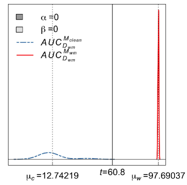
Figure C.1: Population distribution of $AUC_{\mathcal{D}_{wm}}^{\mathcal{M}_{clean}}$ and $AUC_{\mathcal{D}_{wm}}^{\mathcal{M}_{wm}}$ along with the corresponding watermark threshold $t$ with $n=10^{6}$. $\alpha$ and $\beta$ denote the FPR and FNR, while $\mu_{c}$ and $\mu_{w}$ denote the population mean of $AUC_{\mathcal{D}_{wm}}^{\mathcal{M}_{clean}}$ and $AUC_{\mathcal{D}_{wm}}^{\mathcal{M}_{wm}}$.

Appendix D Additional results

Here, we present further results demonstrating the robustness of GENIE. Appendix D.1 lists the results when watermarking was applied to the GraphSAGE model while Appendix D.2 covers the results for the SEAL model. Here, we highlight the value of $AUC_{\mathcal{D}_{wm}}^{\mathcal{M}_{adv}}$ in red if it dropped below the watermark threshold (mention in TABLE III). Appendix D.3 presents additional results for non-ownership piracy test.

D.1 Robustness of GraphSAGE

TABLEs D.1-D.9 present results for different robustness tests for the GraphSAGE model.

TABLE D.1: Impact of model extraction. The architecture of $\mathcal{M}_{adv}$ is the same as $\mathcal{M}_{wm}$, i.e., GraphSAGE.

Dataset		C.ele	USAir	NS	Yeast	Power	arXiv	PPI
Before model extraction	$AUC_{\mathcal{D}_{test}}^{\mathcal{M}_{wm}}$ (%)	86.46	91.89	94.35	90.44	91.23	99.40	94.57
	$AUC_{\mathcal{D}_{wm}}^{\mathcal{M}_{wm}}$ (%)	100.00	100.00	99.77	100.00	99.00	100.00	100.00
After soft extraction	$AUC_{\mathcal{D}_{test}}^{\mathcal{M}_{adv}}$ (%)	86.69	92.75	92.50	90.70	93.29	99.41	94.68
	$AUC_{\mathcal{D}_{wm}}^{\mathcal{M}_{adv}}$ (%)	100.00	76.33	96.66	100.00	95.00	95.42	100.00
After hard extraction	$AUC_{\mathcal{D}_{test}}^{\mathcal{M}_{adv}}$ (%)	85.65	90.20	89.74	90.94	90.86	99.28	94.28
	$AUC_{\mathcal{D}_{wm}}^{\mathcal{M}_{adv}}$ (%)	95.31	56.21	93.11	100.00	91.00	95.03	100.00

TABLE D.2: Impact of knowledge distillation.

Dataset		C.ele	USAir	NS	Yeast	Power	arXiv	PPI
Before distillation	$AUC_{\mathcal{D}_{test}}^{\mathcal{M}_{wm}}$ (%)	86.46	91.89	94.35	90.44	91.23	99.40	94.57
	$AUC_{\mathcal{D}_{wm}}^{\mathcal{M}_{wm}}$ (%)	100.00	100.00	99.77	100.00	99.00	100.00	100.00
After distillation	$AUC_{\mathcal{D}_{test}}^{\mathcal{M}_{adv}}$ (%)	87.37	92.31	88.89	90.55	91.30	99.48	94.79
	$AUC_{\mathcal{D}_{wm}}^{\mathcal{M}_{adv}}$ (%)	81.25	50.30	71.78	98.82	90.00	89.44	100.00

TABLE D.3: Impact of model fine-tuning.

Dataset		Fine-tuning Method
		$\text{No fine-tuning}^{\star}$	FTLL	RTLL	FTAL	RTAL
C.ele	$AUC_{\mathcal{D}_{test}}^{\mathcal{M}_{adv}}$ (%)	86.46	88.92	84.37	82.75	76.51
	$AUC_{\mathcal{D}_{wm}}^{\mathcal{M}_{adv}}$ (%)	100.00	100.0	92.19	85.94	90.62
USAir	$AUC_{\mathcal{D}_{test}}^{\mathcal{M}_{adv}}$ (%)	91.89	90.63	90.27	90.29	88.47
	$AUC_{\mathcal{D}_{wm}}^{\mathcal{M}_{adv}}$ (%)	100.00	100.0	97.63	98.22	86.39
NS	$AUC_{\mathcal{D}_{test}}^{\mathcal{M}_{adv}}$ (%)	94.35	93.63	93.31	91.31	89.71
	$AUC_{\mathcal{D}_{wm}}^{\mathcal{M}_{adv}}$ (%)	99.77	99.33	98.44	84.22	80.22
Yeast	$AUC_{\mathcal{D}_{test}}^{\mathcal{M}_{adv}}$ (%)	90.44	90.37	89.71	88.98	85.89
	$AUC_{\mathcal{D}_{wm}}^{\mathcal{M}_{adv}}$ (%)	100.00	100.00	100.00	99.41	99.41
Power	$AUC_{\mathcal{D}_{test}}^{\mathcal{M}_{adv}}$ (%)	91.23	94.34	94.12	92.16	89.16
	$AUC_{\mathcal{D}_{wm}}^{\mathcal{M}_{adv}}$ (%)	99.00	99.00	93.00	59.00	51.00
arXiv	$AUC_{\mathcal{D}_{test}}^{\mathcal{M}_{adv}}$ (%)	99.40	99.46	99.31	99.43	99.26
	$AUC_{\mathcal{D}_{wm}}^{\mathcal{M}_{adv}}$ (%)	100.00	99.88	69.14	19.66	16.58
PPI	$AUC_{\mathcal{D}_{test}}^{\mathcal{M}_{adv}}$ (%)	94.57	94.73	93.96	93.93	92.54
	$AUC_{\mathcal{D}_{wm}}^{\mathcal{M}_{adv}}$ (%)	100.00	100.00	100.00	39.67	52.07
Column with ⋆ shows the values when $\mathcal{M}_{adv}$ = $\mathcal{M}_{wm}$.

TABLE D.4: Impact of model pruning.

Dataset		Prune Percentage (%)
		$\text{No Pruning}^{\star}$	20	40	60	80	100
C.ele	$AUC_{\mathcal{D}_{test}}^{\mathcal{M}_{adv}}$ (%)	86.46	86.31	85.59	83.50	76.10	50.00
	$AUC_{\mathcal{D}_{wm}}^{\mathcal{M}_{adv}}$ (%)	100.0	100.0	100.0	100.0	79.68	50.00
USAir	$AUC_{\mathcal{D}_{test}}^{\mathcal{M}_{adv}}$ (%)	91.89	91.90	91.83	91.73	88.71	50.00
	$AUC_{\mathcal{D}_{wm}}^{\mathcal{M}_{adv}}$ (%)	100.0	100.0	100.0	100.0	95.85	50.00
NS	$AUC_{\mathcal{D}_{test}}^{\mathcal{M}_{adv}}$ (%)	94.35	94.26	94.42	93.55	86.64	50.00
	$AUC_{\mathcal{D}_{wm}}^{\mathcal{M}_{adv}}$ (%)	99.77	99.77	99.77	98.44	86.88	50.50
Yeast	$AUC_{\mathcal{D}_{test}}^{\mathcal{M}_{adv}}$ (%)	90.44	90.30	89.86	88.33	75.85	50.00
	$AUC_{\mathcal{D}_{wm}}^{\mathcal{M}_{adv}}$ (%)	100.0	100.0	100.0	100.0	66.86	50.00
Power	$AUC_{\mathcal{D}_{test}}^{\mathcal{M}_{adv}}$ (%)	91.23	91.16	91.08	89.72	79.45	50.00
	$AUC_{\mathcal{D}_{wm}}^{\mathcal{M}_{adv}}$ (%)	99.00	99.00	99.00	97.00	93.00	50.00
arXiv	$AUC_{\mathcal{D}_{test}}^{\mathcal{M}_{adv}}$ (%)	99.40	99.40	99.35	99.00	93.91	50.00
	$AUC_{\mathcal{D}_{wm}}^{\mathcal{M}_{adv}}$ (%)	100.00	100.00	100.00	65.25	52.67	50.00
PPI	$AUC_{\mathcal{D}_{test}}^{\mathcal{M}_{adv}}$ (%)	94.57	94.57	94.23	92.84	83.62	50.00
	$AUC_{\mathcal{D}_{wm}}^{\mathcal{M}_{adv}}$ (%)	100.00	100.00	100.00	99.90	21.12	50.00
Column with ⋆ shows the values when $\mathcal{M}_{adv}$ = $\mathcal{M}_{wm}$.

TABLE D.5: Impact of weight quantization.

Dataset		C.ele	USAir	NS	Yeast	Power	arXiv	PPI
Before quantization	$AUC_{\mathcal{D}_{test}}^{\mathcal{M}_{wm}}$ (%)	86.46	91.89	94.35	90.44	91.23	99.40	94.57
	$AUC_{\mathcal{D}_{wm}}^{\mathcal{M}_{wm}}$ (%)	100.00	100.00	99.77	100.00	99.00	100.00	100.00
After quantization	$AUC_{\mathcal{D}_{test}}^{\mathcal{M}_{adv}}$ (%)	83.09	91.09	92.23	89.98	91.49	97.27	92.69
	$AUC_{\mathcal{D}_{wm}}^{\mathcal{M}_{adv}}$ (%)	100.00	100.00	98.89	100.00	99.00	73.80	98.26

TABLE D.6: Impact of pruning + FTLL.

Dataset		Prune Percentage (%)
		$\text{No Pruning}^{\star}$	20	40	60	80
C.ele	$AUC_{\mathcal{D}_{test}}^{\mathcal{M}_{adv}}$ (%)	86.46	89.21	88.73	87.50	87.59
	$AUC_{\mathcal{D}_{wm}}^{\mathcal{M}_{adv}}$ (%)	100.00	100.00	100.00	100.00	87.50
USAir	$AUC_{\mathcal{D}_{test}}^{\mathcal{M}_{adv}}$ (%)	91.90	88.66	87.99	87.15	85.60
	$AUC_{\mathcal{D}_{wm}}^{\mathcal{M}_{adv}}$ (%)	100.0	100.0	100.0	100.0	88.16
NS	$AUC_{\mathcal{D}_{test}}^{\mathcal{M}_{adv}}$ (%)	94.35	88.45	88.06	86.72	77.80
	$AUC_{\mathcal{D}_{wm}}^{\mathcal{M}_{adv}}$ (%)	99.77	99.33	99.33	99.33	89.11
Yeast	$AUC_{\mathcal{D}_{test}}^{\mathcal{M}_{adv}}$ (%)	90.44	90.38	90.27	90.05	88.85
	$AUC_{\mathcal{D}_{wm}}^{\mathcal{M}_{adv}}$ (%)	100.0	100.0	100.0	98.81	67.45
Power	$AUC_{\mathcal{D}_{test}}^{\mathcal{M}_{adv}}$ (%)	91.23	94.38	94.20	94.25	92.37
	$AUC_{\mathcal{D}_{wm}}^{\mathcal{M}_{adv}}$ (%)	99.00	99.00	99.00	99.00	83.00
arXiv	$AUC_{\mathcal{D}_{test}}^{\mathcal{M}_{adv}}$ (%)	99.40	99.45	99.42	99.33	98.56
	$AUC_{\mathcal{D}_{wm}}^{\mathcal{M}_{adv}}$ (%)	100.00	98.54	81.71	25.61	19.29
PPI	$AUC_{\mathcal{D}_{test}}^{\mathcal{M}_{adv}}$ (%)	94.57	94.74	94.61	94.36	91.92
	$AUC_{\mathcal{D}_{wm}}^{\mathcal{M}_{adv}}$ (%)	100.0	100.0	100.0	84.48	57.66
Column with ⋆ shows the values when $\mathcal{M}_{adv}$ = $\mathcal{M}_{wm}$.

TABLE D.7: Impact of pruning + RTLL.

Dataset		Prune Percentage (%)
		$\text{No Pruning}^{\star}$	20	40	60	80
C.ele	$AUC_{\mathcal{D}_{test}}^{\mathcal{M}_{adv}}$ (%)	86.46	84.31	84.56	84.96	85.55
	$AUC_{\mathcal{D}_{wm}}^{\mathcal{M}_{adv}}$ (%)	100.00	92.19	87.50	85.93	65.62
USAir	$AUC_{\mathcal{D}_{test}}^{\mathcal{M}_{adv}}$ (%)	91.90	90.39	90.71	90.25	88.48
	$AUC_{\mathcal{D}_{wm}}^{\mathcal{M}_{adv}}$ (%)	100.00	97.04	97.04	94.08	68.63
NS	$AUC_{\mathcal{D}_{test}}^{\mathcal{M}_{adv}}$ (%)	94.35	93.07	93.32	93.17	90.82
	$AUC_{\mathcal{D}_{wm}}^{\mathcal{M}_{adv}}$ (%)	99.77	98.44	98.88	98.88	90.44
Yeast	$AUC_{\mathcal{D}_{test}}^{\mathcal{M}_{adv}}$ (%)	90.44	89.67	89.49	89.38	88.64
	$AUC_{\mathcal{D}_{wm}}^{\mathcal{M}_{adv}}$ (%)	100.0	100.0	100.0	96.44	70.41
Power	$AUC_{\mathcal{D}_{test}}^{\mathcal{M}_{adv}}$ (%)	91.23	94.02	93.98	93.77	89.57
	$AUC_{\mathcal{D}_{wm}}^{\mathcal{M}_{adv}}$ (%)	99.00	95.00	94.00	99.00	83.00
arXiv	$AUC_{\mathcal{D}_{test}}^{\mathcal{M}_{adv}}$ (%)	99.40	99.30	99.26	99.13	97.98
	$AUC_{\mathcal{D}_{wm}}^{\mathcal{M}_{adv}}$ (%)	100.00	63.95	54.92	32.71	17.43
PPI	$AUC_{\mathcal{D}_{test}}^{\mathcal{M}_{adv}}$ (%)	94.57	93.94	93.76	93.48	90.09
	$AUC_{\mathcal{D}_{wm}}^{\mathcal{M}_{adv}}$ (%)	100.0	100.0	98.89	93.02	49.67
Column with ⋆ shows the values when $\mathcal{M}_{adv}$ = $\mathcal{M}_{wm}$.

TABLE D.8: Impact of pruning + FTAL.

Dataset		Prune Percentage (%)
		$\text{No Pruning}^{\star}$	20	40	60	80
C.ele	$AUC_{\mathcal{D}_{test}}^{\mathcal{M}_{adv}}$ (%)	86.46	82.78	83.11	81.20	79.62
	$AUC_{\mathcal{D}_{wm}}^{\mathcal{M}_{adv}}$ (%)	100.00	96.87	73.43	85.93	68.75
USAir	$AUC_{\mathcal{D}_{test}}^{\mathcal{M}_{adv}}$ (%)	91.89	89.29	89.63	88.75	89.27
	$AUC_{\mathcal{D}_{wm}}^{\mathcal{M}_{adv}}$ (%)	100.00	96.44	94.08	90.53	59.76
NS	$AUC_{\mathcal{D}_{test}}^{\mathcal{M}_{adv}}$ (%)	94.35	92.63	91.31	91.71	88.10
	$AUC_{\mathcal{D}_{wm}}^{\mathcal{M}_{adv}}$ (%)	99.77	91.77	85.55	96.22	82.44
Yeast	$AUC_{\mathcal{D}_{test}}^{\mathcal{M}_{adv}}$ (%)	90.44	89.26	88.50	88.45	87.12
	$AUC_{\mathcal{D}_{wm}}^{\mathcal{M}_{adv}}$ (%)	100.00	98.22	100.00	97.63	82.24
Power	$AUC_{\mathcal{D}_{test}}^{\mathcal{M}_{adv}}$ (%)	91.23	92.30	92.08	92.15	91.96
	$AUC_{\mathcal{D}_{wm}}^{\mathcal{M}_{adv}}$ (%)	99.00	58.00	58.00	67.00	40.00
arXiv	$AUC_{\mathcal{D}_{test}}^{\mathcal{M}_{adv}}$ (%)	99.40	99.42	99.41	99.39	99.24
	$AUC_{\mathcal{D}_{wm}}^{\mathcal{M}_{adv}}$ (%)	100.00	19.64	17.62	15.71	5.42
PPI	$AUC_{\mathcal{D}_{test}}^{\mathcal{M}_{adv}}$ (%)	94.57	93.79	93.90	93.64	93.06
	$AUC_{\mathcal{D}_{wm}}^{\mathcal{M}_{adv}}$ (%)	100.00	40.95	35.16	17.44	22.40
Column with ⋆ shows the values when $\mathcal{M}_{adv}$ = $\mathcal{M}_{wm}$.

TABLE D.9: Impact of pruning + RTAL.

Dataset		Prune Percentage (%)
		$\text{No Pruning}^{\star}$	20	40	60	80
C.ele	$AUC_{\mathcal{D}_{test}}^{\mathcal{M}_{adv}}$ (%)	86.46	82.78	83.11	81.20	79.62
	$AUC_{\mathcal{D}_{wm}}^{\mathcal{M}_{adv}}$ (%)	100.00	92.19	82.81	79.69	73.44
USAir	$AUC_{\mathcal{D}_{test}}^{\mathcal{M}_{adv}}$ (%)	91.89	88.66	87.99	87.15	85.60
	$AUC_{\mathcal{D}_{wm}}^{\mathcal{M}_{adv}}$ (%)	100.00	85.20	81.06	72.18	49.11
NS	$AUC_{\mathcal{D}_{test}}^{\mathcal{M}_{adv}}$ (%)	94.35	92.63	91.31	91.71	88.10
	$AUC_{\mathcal{D}_{wm}}^{\mathcal{M}_{adv}}$ (%)	99.77	91.77	85.55	96.22	82.44
Yeast	$AUC_{\mathcal{D}_{test}}^{\mathcal{M}_{adv}}$ (%)	90.44	86.04	85.18	84.88	83.34
	$AUC_{\mathcal{D}_{wm}}^{\mathcal{M}_{adv}}$ (%)	100.00	99.40	95.85	92.89	71.00
Power	$AUC_{\mathcal{D}_{test}}^{\mathcal{M}_{adv}}$ (%)	91.23	88.95	88.40	87.79	82.69
	$AUC_{\mathcal{D}_{wm}}^{\mathcal{M}_{adv}}$ (%)	99.00	50.99	36.00	43.00	62.99
arXiv	$AUC_{\mathcal{D}_{test}}^{\mathcal{M}_{adv}}$ (%)	99.40	99.25	99.25	99.15	98.83
	$AUC_{\mathcal{D}_{wm}}^{\mathcal{M}_{adv}}$ (%)	100.00	15.27	14.50	9.29	4.65
PPI	$AUC_{\mathcal{D}_{test}}^{\mathcal{M}_{adv}}$ (%)	94.57	92.62	92.26	91.99	90.51
	$AUC_{\mathcal{D}_{wm}}^{\mathcal{M}_{adv}}$ (%)	100.00	48.57	41.05	50.87	36.17
Column with ⋆ shows the values when $\mathcal{M}_{adv}$ = $\mathcal{M}_{wm}$.

D.2 Robustness of SEAL

TABLEs D.10-D.16 present results for different robustness tests for the SEAL model.

TABLE D.10: Impact of model fine-tuning.

Dataset		Fine tuning Method
		$\text{No fine-tuning}^{\star}$	FTLL	RTLL	FTAL	RTAL
C.ele	$AUC_{\mathcal{D}_{test}}^{\mathcal{M}_{adv}}$ (%)	88.50	89.88	90.07	88.21	88.88
	$AUC_{\mathcal{D}_{wm}}^{\mathcal{M}_{adv}}$ (%)	84.27	84.30	84.16	83.47	83.94
USAir	$AUC_{\mathcal{D}_{test}}^{\mathcal{M}_{adv}}$ (%)	95.66	93.81	93.05	93.08	92.49
	$AUC_{\mathcal{D}_{wm}}^{\mathcal{M}_{adv}}$ (%)	92.35	92.46	91.47	91.79	88.03
NS	$AUC_{\mathcal{D}_{test}}^{\mathcal{M}_{adv}}$ (%)	98.61	98.46	98.32	99.25	98.94
	$AUC_{\mathcal{D}_{wm}}^{\mathcal{M}_{adv}}$ (%)	98.77	98.77	98.78	97.44	58.26
Yeast	$AUC_{\mathcal{D}_{test}}^{\mathcal{M}_{adv}}$ (%)	97.06	97.05	97.14	96.35	96.07
	$AUC_{\mathcal{D}_{wm}}^{\mathcal{M}_{adv}}$ (%)	96.34	96.35	95.49	94.73	91.95
Power	$AUC_{\mathcal{D}_{test}}^{\mathcal{M}_{adv}}$ (%)	85.64	87.31	87.49	84.20	83.08
	$AUC_{\mathcal{D}_{wm}}^{\mathcal{M}_{adv}}$ (%)	88.78	88.78	88.65	57.04	18.36
Column with ⋆ shows the values when $\mathcal{M}_{adv}$ = $\mathcal{M}_{wm}$.

TABLE D.11: Impact of model pruning.

Dataset		Prune Percentage (%)
		$\text{No Pruning}^{\star}$	20	40	60	80	100
C.ele	$AUC_{\mathcal{D}_{test}}^{\mathcal{M}_{adv}}$ (%)	88.50	88.63	88.60	88.48	87.93	50.0
	$AUC_{\mathcal{D}_{wm}}^{\mathcal{M}_{adv}}$ (%)	84.27	83.97	83.93	84.09	83.17	50.0
USAir	$AUC_{\mathcal{D}_{test}}^{\mathcal{M}_{adv}}$ (%)	95.66	95.61	95.81	95.53	95.25	50.0
	$AUC_{\mathcal{D}_{wm}}^{\mathcal{M}_{adv}}$ (%)	92.35	92.31	92.24	91.40	91.56	50.0
NS	$AUC_{\mathcal{D}_{test}}^{\mathcal{M}_{adv}}$ (%)	98.61	98.52	97.97	95.59	84.69	50.0
	$AUC_{\mathcal{D}_{wm}}^{\mathcal{M}_{adv}}$ (%)	98.77	98.78	97.58	97.53	95.19	50.0
Yeast	$AUC_{\mathcal{D}_{test}}^{\mathcal{M}_{adv}}$ (%)	97.06	97.08	97.14	96.96	96.81	50.0
	$AUC_{\mathcal{D}_{wm}}^{\mathcal{M}_{adv}}$ (%)	96.34	96.33	96.27	92.66	93.37	50.0
Power	$AUC_{\mathcal{D}_{test}}^{\mathcal{M}_{adv}}$ (%)	85.64	85.23	84.68	83.80	45.49	50.0
	$AUC_{\mathcal{D}_{wm}}^{\mathcal{M}_{adv}}$ (%)	88.78	88.63	87.98	76.88	78.99	50.0
Column with ⋆ shows the values when $\mathcal{M}_{adv}$ = $\mathcal{M}_{wm}$.

TABLE D.12: Impact of weight quantization.

Dataset		C.ele	USAir	NS	Yeast	Power
Before quantization	$AUC_{\mathcal{D}_{test}}^{\mathcal{M}_{wm}}$ (%)	88.50	95.66	98.61	97.06	85.64
	$AUC_{\mathcal{D}_{wm}}^{\mathcal{M}_{wm}}$ (%)	84.27	92.35	98.77	96.34	88.78
After quantization	$AUC_{\mathcal{D}_{test}}^{\mathcal{M}_{adv}}$ (%)	84.34	91.97	98.42	90.97	80.58
	$AUC_{\mathcal{D}_{wm}}^{\mathcal{M}_{adv}}$ (%)	80.32	87.48	76.37	91.10	87.61

TABLE D.13: Impact of pruning + FTLL.

Dataset		Prune Percentage (%)
		$\text{No Pruning}^{\star}$	20	40	60	80
C.ele	$AUC_{\mathcal{D}_{test}}^{\mathcal{M}_{adv}}$ (%)	88.50	89.82	90.05	89.83	89.41
	$AUC_{\mathcal{D}_{wm}}^{\mathcal{M}_{adv}}$ (%)	84.27	83.99	83.97	84.13	83.24
USAir	$AUC_{\mathcal{D}_{test}}^{\mathcal{M}_{adv}}$ (%)	95.66	93.72	93.90	93.33	93.09
	$AUC_{\mathcal{D}_{wm}}^{\mathcal{M}_{adv}}$ (%)	92.35	92.43	92.31	91.43	91.59
NS	$AUC_{\mathcal{D}_{test}}^{\mathcal{M}_{adv}}$ (%)	98.61	98.35	98.05	95.74	88.73
	$AUC_{\mathcal{D}_{wm}}^{\mathcal{M}_{adv}}$ (%)	98.77	98.76	97.60	97.40	92.36
Yeast	$AUC_{\mathcal{D}_{test}}^{\mathcal{M}_{adv}}$ (%)	97.06	97.03	97.11	96.88	96.61
	$AUC_{\mathcal{D}_{wm}}^{\mathcal{M}_{adv}}$ (%)	96.34	96.33	96.27	92.75	93.18
Power	$AUC_{\mathcal{D}_{test}}^{\mathcal{M}_{adv}}$ (%)	85.64	87.47	87.08	86.20	53.21
	$AUC_{\mathcal{D}_{wm}}^{\mathcal{M}_{adv}}$ (%)	88.78	88.63	87.96	76.97	65.68
Column with ⋆ shows the values when $\mathcal{M}_{adv}$ = $\mathcal{M}_{wm}$.

TABLE D.14: Impact of pruning + RTLL.

Dataset		Prune Percentage (%)
		$\text{No Pruning}^{\star}$	20	40	60	80
C.ele	$AUC_{\mathcal{D}_{test}}^{\mathcal{M}_{adv}}$ (%)	88.50	90.10	90.26	90.29	89.77
	$AUC_{\mathcal{D}_{wm}}^{\mathcal{M}_{adv}}$ (%)	84.27	84.03	83.94	84.21	83.42
USAir	$AUC_{\mathcal{D}_{test}}^{\mathcal{M}_{adv}}$ (%)	95.66	93.17	93.39	93.34	92.92
	$AUC_{\mathcal{D}_{wm}}^{\mathcal{M}_{adv}}$ (%)	92.35	91.60	91.05	90.45	90.52
NS	$AUC_{\mathcal{D}_{test}}^{\mathcal{M}_{adv}}$ (%)	98.61	98.26	98.01	96.48	93.81
	$AUC_{\mathcal{D}_{wm}}^{\mathcal{M}_{adv}}$ (%)	98.77	98.73	98.02	91.95	54.30
Yeast	$AUC_{\mathcal{D}_{test}}^{\mathcal{M}_{adv}}$ (%)	97.06	97.11	97.17	96.88	96.62
	$AUC_{\mathcal{D}_{wm}}^{\mathcal{M}_{adv}}$ (%)	96.34	95.41	95.43	91.17	92.36
Power	$AUC_{\mathcal{D}_{test}}^{\mathcal{M}_{adv}}$ (%)	85.64	87.44	87.24	86.56	81.25
	$AUC_{\mathcal{D}_{wm}}^{\mathcal{M}_{adv}}$ (%)	88.78	88.48	87.85	73.94	22.01
Column with ⋆ shows the values when $\mathcal{M}_{adv}$ = $\mathcal{M}_{wm}$.

TABLE D.15: Impact of pruning + FTAL.

Dataset		Prune Percentage (%)
		$\text{No Pruning}^{\star}$	20	40	60	80
C.ele	$AUC_{\mathcal{D}_{test}}^{\mathcal{M}_{adv}}$ (%)	88.50	88.38	88.42	89.07	89.45
	$AUC_{\mathcal{D}_{wm}}^{\mathcal{M}_{adv}}$ (%)	84.27	83.09	83.38	82.60	82.66
USAir	$AUC_{\mathcal{D}_{test}}^{\mathcal{M}_{adv}}$ (%)	95.66	93.02	92.78	93.22	92.50
	$AUC_{\mathcal{D}_{wm}}^{\mathcal{M}_{adv}}$ (%)	92.35	91.80	91.70	91.31	90.38
NS	$AUC_{\mathcal{D}_{test}}^{\mathcal{M}_{adv}}$ (%)	98.61	99.12	99.25	98.91	98.06
	$AUC_{\mathcal{D}_{wm}}^{\mathcal{M}_{adv}}$ (%)	98.77	96.77	90.93	31.87	6.04
Yeast	$AUC_{\mathcal{D}_{test}}^{\mathcal{M}_{adv}}$ (%)	97.06	96.39	96.41	96.27	95.99
	$AUC_{\mathcal{D}_{wm}}^{\mathcal{M}_{adv}}$ (%)	96.34	95.00	94.23	93.56	94.39
Power	$AUC_{\mathcal{D}_{test}}^{\mathcal{M}_{adv}}$ (%)	85.64	84.56	84.20	83.41	82.35
	$AUC_{\mathcal{D}_{wm}}^{\mathcal{M}_{adv}}$ (%)	88.78	66.32	86.24	49.40	15.61
Column with ⋆ shows the values when $\mathcal{M}_{adv}$ = $\mathcal{M}_{wm}$.

TABLE D.16: Impact of pruning + RTAL.

Dataset		Prune Percentage (%)
		$\text{No Pruning}^{\star}$	20	40	60	80
C.ele	$AUC_{\mathcal{D}_{test}}^{\mathcal{M}_{adv}}$ (%)	88.50	88.86	88.71	88.54	88.75
	$AUC_{\mathcal{D}_{wm}}^{\mathcal{M}_{adv}}$ (%)	84.27	83.73	83.80	83.73	82.76
USAir	$AUC_{\mathcal{D}_{test}}^{\mathcal{M}_{adv}}$ (%)	95.66	92.50	92.44	92.32	92.30
	$AUC_{\mathcal{D}_{wm}}^{\mathcal{M}_{adv}}$ (%)	92.35	88.25	88.18	87.87	86.83
NS	$AUC_{\mathcal{D}_{test}}^{\mathcal{M}_{adv}}$ (%)	98.61	98.96	98.82	98.34	97.87
	$AUC_{\mathcal{D}_{wm}}^{\mathcal{M}_{adv}}$ (%)	98.77	55.80	42.97	20.32	5.03
Yeast	$AUC_{\mathcal{D}_{test}}^{\mathcal{M}_{adv}}$ (%)	97.06	95.93	95.95	95.92	95.93
	$AUC_{\mathcal{D}_{wm}}^{\mathcal{M}_{adv}}$ (%)	96.34	92.69	93.34	92.99	92.92
Power	$AUC_{\mathcal{D}_{test}}^{\mathcal{M}_{adv}}$ (%)	85.64	82.71	82.70	82.76	82.63
	$AUC_{\mathcal{D}_{wm}}^{\mathcal{M}_{adv}}$ (%)	88.78	16.03	13.56	11.73	12.97
Column with ⋆ shows the values when $\mathcal{M}_{adv}$ = $\mathcal{M}_{wm}$.

D.3 Further results for non-ownership piracy

Due to the page length limit, we could only include results for one dataset for non-ownership piracy test in the main text. Now, we present the results for the other datasets in Figure D.1.

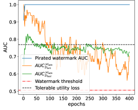
(a) C.ele

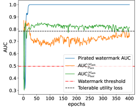
(b) USAir

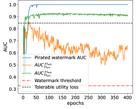
(c) PPI

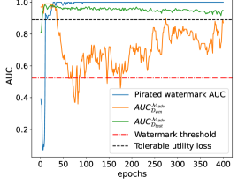
(d) Power

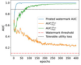
(e) arXiv

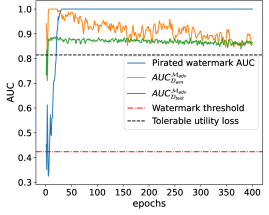
(f) Yeast

Figure D.1: Non-ownership piracy test for GCN model on different datasets.

Appendix E GENIE’s performance on additional datasets

We have conducted a preliminary testing on 3 additional datasets of varying sizes, i.e., ogbl-collab [68], Wikipedia [69], and Router [70]. ogbl-collab is an author collaboration network with 235,868 nodes and 1,285,465 edges. Wikipedia dataset has 4,777 nodes, 184,812 edges, and 40 attributes. Router is a router-level Internet network dataset with 5,022 nodes and 6,258 edges.

TABLE E.1 shows $AUC_{\mathcal{D}_{test}}^{\mathcal{M}_{clean}}$, $AUC_{\mathcal{D}_{test}}^{\mathcal{M}_{wm}}$, and $AUC_{\mathcal{D}_{wm}}^{\mathcal{M}_{wm}}$. We observe that GENIE could successfully watermark the model with minimal utility loss, which indicates that GENIE satisfies functionality preservation requirements on these datasets as well. We keep further testing (e.g., robustness tests, efficiency tests) of GENIE on these datasets as part of our future work.

TABLE E.1: Watermark verification performance (average of 10 runs) of GENIE across 3 model architectures and 3 additional datasets.

Dataset	SEAL			GCN			GraphSAGE
	$AUC_{\mathcal{D}_{test}}^{\mathcal{M}_{clean}}$ (%)	$AUC_{\mathcal{D}_{test}}^{\mathcal{M}_{wm}}$ (%)	$AUC_{\mathcal{D}_{wm}}^{\mathcal{M}_{wm}}$ (%)	$AUC_{\mathcal{D}_{test}}^{\mathcal{M}_{clean}}$ (%)	$AUC_{\mathcal{D}_{test}}^{\mathcal{M}_{wm}}$ (%)	$AUC_{\mathcal{D}_{wm}}^{\mathcal{M}_{wm}}$ (%)	$AUC_{\mathcal{D}_{test}}^{\mathcal{M}_{clean}}$ (%)	$AUC_{\mathcal{D}_{test}}^{\mathcal{M}_{wm}}$ (%)	$AUC_{\mathcal{D}_{wm}}^{\mathcal{M}_{wm}}$ (%)
Router [70]	95.68	95.86	96.22	96.75	96.53	95.23	92.85	96.27	95.44
ogbl-collab [68]	95.56	95.17	99.92	96.39	100.00	95.71	96.94	100.00	95.79
Wikipedia [69]	91.12	91.13	84.72	92.09	90.21	99.58	93.24	92.91	100.00

References

- [1] K. He, X. Zhang, S. Ren, and J. Sun, “Deep Residual Learning for Image Recognition,” in CVPR, 2016, pp. 770–778.
- [2] K. Simonyan and A. Zisserman, “Very Deep Convolutional Networks for Large-Scale Image Recognition,” arXiv preprint:1409.1556, 2014.
- [3] A. Vaswani, N. Shazeer, N. Parmar, J. Uszkoreit, L. Jones, A. N. Gomez, Ł. Kaiser, and I. Polosukhin, “Attention is All you Need,” NeurIPS, vol. 30, 2017.
- [4] W. Fan, Y. Ma, Q. Li, Y. He, E. Zhao, J. Tang, and D. Yin, “Graph Neural Networks for Social Recommendation,” in WWW, 2019, pp. 417–426.
- [5] W. Jiang and J. Luo, “Graph Neural Network for Traffic Forecasting: A Survey,” Expert Systems with Applications, p. 117921, 2022.
- [6] A. Chaudhary, H. Mittal, and A. Arora, “Anomaly Detection using Graph Neural Networks,” in COMITCon. IEEE, 2019, pp. 346–350.
- [7] D. Jiang, Z. Wu, C.-Y. Hsieh, G. Chen, B. Liao, Z. Wang, C. Shen, D. Cao, J. Wu, and T. Hou, “Could Graph Neural Networks learn better Molecular Representation for Drug Discovery? A Comparison Study of Descriptor-Based and Graph-Based Models,” Journal of Cheminformatics, vol. 13, pp. 1–23, 2021.
- [8] T. N. Kipf and M. Welling, “Semi-Supervised Classification with Graph Convolutional Networks,” arXiv preprint:1609.02907, 2016.
- [9] S. Motie and B. Raahemi, “Financial Fraud Detection using Graph Neural Networks: A Systematic Review,” Expert Systems With Applications, p. 122156, 2023.
- [10] K. Jha, S. Saha, and H. Singh, “Prediction of Protein–Protein Interaction using Graph Neural Networks,” Scientific Reports, vol. 12, no. 1, p. 8360, 2022.
- [11] N. N. Daud, S. H. Ab Hamid, M. Saadoon, F. Sahran, and N. B. Anuar, “Applications of Link Prediction in Social Networks: A Review,” Elsevier JNCA, vol. 166, p. 102716, 2020.
- [12] Y. Shen, X. He, Y. Han, and Y. Zhang, “Model Stealing Attacks against Inductive Graph Neural Networks,” in IEEE S&P, 2022, pp. 1175–1192.
- [13] D. DeFazio and A. Ramesh, “Adversarial Model Extraction on Graph Neural Networks,” arXiv preprint:1912.07721, 2019.
- [14] B. Wu, X. Yang, S. Pan, and X. Yuan, “Model Extraction Attacks on Graph Neural Networks: Taxonomy And Realisation,” in ASIACCS, 2022, pp. 337–350.
- [15] Y. Li, H. Wang, and M. Barni, “A Survey of Deep Neural Network Watermarking Techniques,” NeuroComputing, vol. 461, pp. 171–193, 2021.
- [16] Y. Adi, C. Baum, M. Cisse, B. Pinkas, and J. Keshet, “Turning Your Weakness Into a Strength: Watermarking Deep Neural Networks by Backdooring,” in USENIX Security, 2018, pp. 1615–1631.
- [17] F. Boenisch, “A Systematic Review on Model Watermarking for Neural Networks,” Frontiers in Big Data, vol. 4, p. 729663, 2021.
- [18] X. Zhao, H. Wu, and X. Zhang, “Watermarking Graph Neural Networks by Random Graphs,” in IEEE ISDFS, 2021, pp. 1–6.
- [19] J. Xu, S. Koffas, O. Ersoy, and S. Picek, “Watermarking Graph Neural Networks Based on Backdoor Attacks,” in IEEE EuroS&P, 2023, pp. 1179–1197.
- [20] J. Wang, P. Huang, H. Zhao, Z. Zhang, B. Zhao, and D. L. Lee, “Billion-Scale Commodity Embedding for E-Commerce Recommendation in Alibaba,” in KDD, 2018, pp. 839–848.
- [21] R. Ying, R. He, K. Chen, P. Eksombatchai, W. L. Hamilton, and J. Leskovec, “Graph Convolutional Neural Networks for Web-Scale Recommender Systems,” in KDD, 2018, pp. 974–983.
- [22] A. Lerer, L. Wu, J. Shen, T. Lacroix, L. Wehrstedt, A. Bose, and A. Peysakhovich, “Pytorch-Biggraph: A Large Scale Graph Embedding System,” MLSys, pp. 120–131, 2019.
- [23] M. E. Newman, “Clustering and preferential attachment in growing networks,” Physical Review E, vol. 64, no. 2, p. 025102, 2001.
- [24] A. Grover and J. Leskovec, “Node2Vec: Scalable Feature Learning for Networks,” in KDD, 2016, pp. 855–864.
- [25] M. Zhang and Y. Chen, “Link Prediction Based on Graph Neural Networks,” NeurIPS, vol. 31, 2018.
- [26] W. Hamilton, Z. Ying, and J. Leskovec, “Inductive Representation Learning on Large Graphs,” NeurIPS, vol. 30, 2017.
- [27] M. Zhang, Z. Cui, M. Neumann, and Y. Chen, “An End-To-End Deep Learning Architecture for Graph Classification,” in AAAI Conf. on AI, vol. 32, 2018.
- [28] D. Liben-Nowell and J. Kleinberg, “The Link Prediction Problem for Social Networks,” in CIKM, 2003, pp. 556–559.
- [29] A. K. Menon and C. Elkan, “Link Prediction via Matrix Factorization,” in ECML PKDD. Springer, 2011, pp. 437–452.
- [30] Y. Li, Y. Jiang, Z. Li, and S.-T. Xia, “Backdoor Learning: A Survey,” IEEE TNNLS, vol. 35, pp. 5–22, 2022.
- [31] W. Guo, B. Tondi, and M. Barni, “An Overview of Backdoor Attacks against Deep Neural Networks and Possible Defences,” IEEE Open Journal of Signal Processing, vol. 3, pp. 261–287, 2022.
- [32] Z. Xi, R. Pang, S. Ji, and T. Wang, “Graph Backdoor,” in USENIX Security, 2021, pp. 1523–1540.
- [33] J. Xu, M. Xue, and S. Picek, “Explainability-Based Backdoor Attacks against Graph Neural Networks,” in ACM WiseML, 2021, pp. 31–36.
- [34] J. Zhang, Z. Gu, J. Jang, H. Wu, M. P. Stoecklin, H. Huang, and I. Molloy, “Protecting Intellectual Property of Deep Neural Networks with Watermarking,” in ACM ASIACCS, 2018, pp. 159–172.
- [35] N. Lukas, E. Jiang, X. Li, and F. Kerschbaum, “SoK: How Robust is Image Classification Deep Neural Network Watermarking?” in IEEE S&P, 2022, pp. 787–804.
- [36] P. Lv, H. Ma, K. Chen, J. Zhou, S. Zhang, R. Liang, S. Zhu, P. Li, and Y. Zhang, “Mea-Defender: A Robust Watermark against Model Extraction Attack,” arXiv preprint:2401.15239, 2024.
- [37] S. Szyller, B. G. Atli, S. Marchal, and N. Asokan, “Dawn: Dynamic Adversarial Watermarking of Neural Networks,” in ACM MM, 2021, pp. 4417–4425.
- [38] B. Kim, S. Lee, S. Lee, S. Son, and S. J. Hwang, “Margin-Based Neural Network Watermarking,” in ICML, 2023, pp. 16 696–16 711.
- [39] L. A. Adamic and E. Adar, “Friends and Neighbors on the Web,” Social Networks, vol. 25, no. 3, pp. 211–230, 2003.
- [40] Y. Koren, R. Bell, and C. Volinsky, “Matrix Factorization Techniques for Recommender Systems,” Computer, vol. 42, pp. 30–37, 2009.
- [41] T. Oyetunde, M. Zhang, Y. Chen, Y. Tang, and C. Lo, “Boostgapfill: Improving the Fidelity of Metabolic Network Reconstructions through Integrated Constraint and Pattern-Based Methods,” Bioinformatics, vol. 33, no. 4, pp. 608–611, 2017.
- [42] H. Zheng, H. Xiong, H. Ma, G. Huang, and J. Chen, “Link-Backdoor: Backdoor Attack on Link Prediction via Node Injection,” IEEE TCSS, vol. 11, pp. 1816–1831, 2023.
- [43] J. Dai and H. Sun, “A Backdoor Attack against Link Prediction Tasks with Graph Neural Networks,” arXiv preprint:2401.02663, 2024.
- [44] F. A. Petitcolas, R. J. Anderson, and M. G. Kuhn, “Information Hiding - A Survey,” Proceedings of the IEEE, vol. 87, pp. 1062–1078, 1999.
- [45] J.-E. Ekberg, K. Kostiainen, and N. Asokan, “The Untapped Potential of Trusted Execution Environments on Mobile Devices,” IEEE S&P Magazine, vol. 12, no. 4, pp. 29–37, 2014.
- [46] S. Gallagher. (2023) Trusted Compute Base. [Online]. Available: https://learn.microsoft.com/en-us/azure/confidential-computing/trusted-compute-base?source=recommendations
- [47] J. Tan, N. Zhong, Z. Qian, X. Zhang, and S. Li, “Deep Neural Network Watermarking against Model Extraction Attack,” in ACM MM, 2023, pp. 1588–1597.
- [48] B. Efron, “Bootstrap Methods: Another Look at the Jackknife,” The Annals of Statistics, pp. 1–26, 1979.
- [49] B. L. Welch, “The generalization of ‘STUDENT’S’problem when several different population varlances are involved,” Biometrika, vol. 34, no. 1-2, pp. 28–35, 1947.
- [50] “Mann Whitney Test,” in The Concise Encyclopedia of Statistics, 2008, pp. 327–329.
- [51] S. S. Shapiro and M. B. Wilk, “An Analysis of Variance Test for Normality (Complete Samples),” Biometrika, vol. 52, pp. 591–611, 1965. [Online]. Available: http://www.jstor.org/stable/2333709
- [52] C. Von Mering, R. Krause, B. Snel, M. Cornell, S. G. Oliver, S. Fields, and P. Bork, “Comparative Assessment of Large-Scale Data Sets of Protein–Protein Interactions,” Nature, vol. 417, pp. 399–403, 2002.
- [53] B. W. Silverman, Density Estimation for Statistics and Data Analysis. Routledge, 2018.
- [54] D. J. Watts and S. H. Strogatz, “Collective Dynamics of ‘Small-World’Networks,” Nature, vol. 393, no. 6684, pp. 440–442, 1998.
- [55] V. Batagelj and A. Mrvar, “Pajek Datasets: http://vlado. fmf. uni-lj. si/pub/networks/data/mix,” USAir97. net, 2006.
- [56] M. E. Newman, “Finding Community Structure in Networks using the Eigenvectors of Matrices,” Physical Review E, vol. 74, no. 3, p. 036104, 2006.
- [57] L. Jure, “Snap Datasets: Stanford Large Network Dataset Collection,” Retrieved December 2021 from http://snap. stanford. edu/data, 2014.
- [58] C. Stark, B.-J. Breitkreutz, T. Reguly, L. Boucher, A. Breitkreutz, and M. Tyers, “Biogrid: A General Repository for Interaction Datasets,” Nucleic Acids Research, vol. 34, no. suppl_1, pp. D535–D539, 2006.
- [59] A. Paszke, S. Gross, F. Massa, A. Lerer, J. Bradbury, G. Chanan, T. Killeen, Z. Lin, N. Gimelshein, L. Antiga et al., “Pytorch: An Imperative Style, High-Performance Deep Learning Library,” NeurIPS, vol. 32, 2019.
- [60] J. A. Hanley and B. J. McNeil, “The Meaning and Use of the Area Under a Receiver Operating Characteristic (ROC) Curve.” Radiology, vol. 143, pp. 29–36, 1982.
- [61] G. Hinton, O. Vinyals, and J. Dean, “Distilling the Knowledge in a Neural Network,” arXiv preprint:1503.02531, 2015.
- [62] J. Yosinski, J. Clune, Y. Bengio, and H. Lipson, “How Transferable are Features in Deep Neural Networks?” NeurIPS, vol. 27, 2014.
- [63] S. Han, J. Pool, J. Tran, and W. Dally, “Learning both Weights and Connections for Efficient Neural Network,” NeurIPS, vol. 28, 2015.
- [64] A. Gholami, S. Kim, Z. Dong, Z. Yao, M. W. Mahoney, and K. Keutzer, “A Survey of Quantization Methods for Efficient Neural Network Inference,” in Low-Power Computer Vision. CRC, 2022, pp. 291–326.
- [65] M. S. Suraj Subramanian and J. Zhang. (2022) Practical Quantization in PyTorch. [Online]. Available: https://pytorch.org/blog/quantization-in-practice/
- [66] B. Efron and R. J. Tibshirani, An Introduction to The Bootstrap. CRC, 1994, vol. 57.
- [67] E. Parzen, “On Estimation of a Probability Density Function and Mode,” The Annals of Mathematical Statistics, vol. 33, no. 3, pp. 1065–1076, 1962.
- [68] W. Hu, M. Fey, M. Zitnik, Y. Dong, H. Ren, B. Liu, M. Catasta, and J. Leskovec, “Open Graph Benchmark: Datasets for Machine Learning on Graphs,” NeurIPS, vol. 33, pp. 22 118–22 133, 2020.
- [69] M. Mahoney. (2011) Large Text Compression Benchmark. [Online]. Available: https://mattmahoney.net/dc/text.html
- [70] N. Spring, R. Mahajan, D. Wetherall, and T. Anderson, “Measuring ISP Topologies with Rocketfuel,” IEEE ToN, vol. 12, pp. 2–16, 2004.