Crafting Heavy-Tails in Weight Matrix Spectrum
without Gradient Noise

Abstract

Modern training strategies of deep neural networks (NNs) tend to induce a heavy-tailed (HT) spectra of layer weights. Extensive efforts to study this phenomenon have found that NNs with HT weight spectra tend to generalize well. A prevailing notion for the occurrence of such HT spectra attributes gradient noise during training as a key contributing factor. Our work shows that gradient noise is unnecessary for generating HT weight spectra: two-layer NNs trained with full-batch Gradient Descent/Adam can exhibit HT spectra in their weights after finite training steps. To this end, we first identify the scale of the learning rate at which one step of full-batch Adam can lead to feature learning in the shallow NN, particularly when learning a single index teacher model. Next, we show that multiple optimizer steps with such (sufficiently) large learning rates can transition the bulk of the weight’s spectra into an HT distribution. To understand this behavior, we present a novel perspective based on the singular vectors of the weight matrices and optimizer updates. We show that the HT weight spectrum originates from the ‘spike’, which is generated from feature learning and interacts with the main bulk to generate an HT spectrum. Finally, we analyze the correlations between the HT weight spectra and generalization after multiple optimizer updates with varying learning rates.

1 Introduction

Recent efforts on the spectral analysis of NN weights [1, 2, 3, 4, 5, 6] have shown that a well-trained NN tends to exhibit a heavy-tailed (HT) Empirical Spectral Density (ESD) in its weight matrices. Notably, [3] observed this phenomenon by conducting extensive experiments on state-of-the-art deep NNs. Their experiments indicate an HT ‘implicit regularization’ of weights, which seems to be introduced by the stochastic optimization process. Meanwhile, people observed HT phenomenon in the distribution of weights themselves [7, 8, 9, 10, 11, 12] and attribute multiplicative noise or SGD/Adam noise to be the sources. On the other hand, [13] discusses another angle in which overparameterization and interpolation help the weight spectra exhibit heavy tails. While significant progress has been made in recent years, understanding the conditions (architecture, data, training strategy) under which heavy tails emerge remains an open problem.

One of the pressing challenges in understanding the HT phenomenon is the disconnect between practical settings and theoretical analysis, which is rooted in the choice of adaptive optimizers (such as Adam [14]). Owing to its simplicity, most of the theoretical efforts rely on GD/SGD [11, 9, 8], whereas it is common practice to use Adam (and its variants) for training NNs in the modern era [4, 15]. Our work aims to bridge this gap. We employ the widely studied ‘Teacher-Student’ [16, 17, 18, 19, 20, 21, 22, 23, 24, 25, 26, 5, 27, 26, 28] setting to understand the role of optimizer and the scale of learning rates which lead to the HT phenomenon. To this end, we train a two-layer feed-forward NN (Student) in the high-dimensional regime to learn a single-index model (Teacher) [29, 30, 31, 20, 32, 33, 34] using (vanilla) Gradient Descent (GD) and Full-batch Adam (FB-Adam), and convey the following message:

“The ESD of the hidden layer weight matrix exhibits heavy tails after multiple steps of GD/FB-Adam with (sufficiently) large learning rates”.

Our message’s two key aspects comprise: 1. multiple optimizer steps and 2. (sufficiently) large learning rates. Recent works such as [27, 35] have identified the learning rate scale at which one step of GD can allow the student network to learn the target direction of the teacher model. Our work identifies such a learning rate scale for FB-Adam. Furthermore, we show that even $10$ optimizer steps with such large learning rates can induce heavy tails in the spectrum of the hidden layer weight matrix of the student network (see Figure 1).

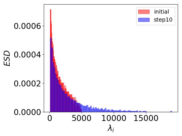
(a) GD $\eta=2000$

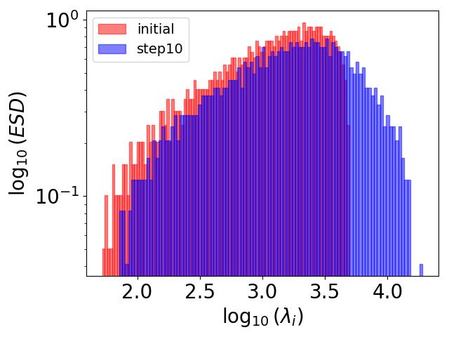
(b) GD $\eta=2000$

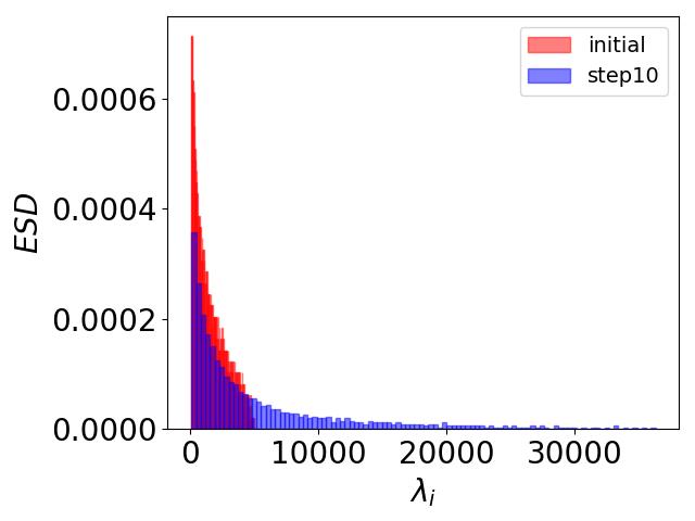
(c) FB-Adam $\eta=0.5$

(d) FB-Adam $\eta=0.5$

Figure 1: Emergence of HT spectra after $10$ GD/FB-Adam steps. Both linear and log scales are shown. For the purpose of illustrating clear HT shapes, we did not choose a highly HT spectrum. Highly HT spectra can also be generated without gradient noise and are discussed in Appendix A.

Previous works that theoretically analyze the role of one-step GD and large learning rates relied heavily on the randomness of the initialized weight matrices [27, 24, 36, 35]. However, the coupling between data and weight matrices after the first update makes it challenging to analyze multiple optimizer steps with the existing techniques. Yet, such an escape from randomness after multiple steps is essential for learning ‘hard’ single index models [28]. In particular, it was recently shown that online (one-pass) SGD can fail to recover the target direction of the single-index teacher model with large ‘Information Exponents’ [17], whereas multi-pass SGD succeeds [28]. Owing to these challenges and benefits of analyzing multi-pass training, we present a novel perspective on HT emergence after multiple optimizer steps using tools from the ‘signal recovery’ literature [37, 38, 39]. In particular, we show that the alignments of singular vectors of the hidden layer weight matrix and its corresponding optimizer update matrix significantly influence the weight matrix ESD. In this context, we study the role of the learning rates, weight normalization, and the choice of the optimizer (GD/FB-Adam) in determining such singular vector alignments and the resulting heavy-tails in the weight matrix spectrum. To summarize, we make the following contributions:

• We identify the scale of the learning rates at which the first FB-Adam update on the hidden layer leads to a spike in the weight matrix ESD, thereby facilitating feature learning in the student network to learn the target direction of the teacher model.

• With such sufficiently large learning rates, we show that “stochastic gradient noise” during optimization is not necessary for the weights of an NN to exhibit HT spectra. In particular, we study the alignments of singular vectors of the weight and corresponding optimizer update matrices as a potential contributor to the emergence of the HT phenomenon.

• We empirically analyze the correlations between the exponent of the power-law distribution that is fit to the weight matrix ESD and the generalization of the student network after multiple optimizer updates. The role of techniques such as weight normalization and learning rate schedules is also analyzed.

2 Related Work

Feature learning.

Due to the limitations of the lazy training regime observed in random feature (RF) and kernel models  [40, 41, 42, 43, 44, 45, 46, 47, 48, 49, 50, 51, 35, 52, 53, 54, 55], recent studies have shifted the focus to exploring feature learning and understanding the training dynamics of NNs. Recently, [27, 35, 36, 56] showed that in the high dimensional regime (i.e the sample size, data dimension, and hidden layer width scale proportionally), a large learning rate [57, 58, 59] is necessary for a two-layer NN to learn the hidden direction of a single-index model after one-step of gradient descent. If the learning rate is too small, the ESD of the weight matrix remains largely unchanged after a single GD update, indicating an inability to learn the target direction effectively. However, when the learning rate exceeds a certain threshold, the ESD of the weight matrix after one step GD update exhibits a spike that contains feature information within its corresponding principal component. Furthermore, recent work by [28] showcases the benefits of multi-pass GD to learn single index models with larger information exponents [17], which cannot be learned by two-layer networks with a single-pass over the data.

Heavy-Tailed phenomenon.

The HT phenomenon in ESDs of weight matrices and the HT distribution of weights has been an active area of study [3, 2, 4, 6, 7, 8, 9, 11]. The driving factor can be attributed to the emergence of HT weight spectra in well-trained NNs with good generalization [3]. To show how ESDs evolve from initialization to HT during training, [1, 3] proposed a ‘$5+1$’ phase model corresponding to the evolution of the bulk and spikes in the ESD. Their study suggests that HT spectrum corresponds to strong correlations between the weight parameters. On the other hand, [7, 8, 9, 11] attribute the emergence of the HT phenomenon to multiplicative or HT gradient noise. Recently, [13] showed that overparameterization and interpolation could be key contributing factors that drive the emergence of HT weight spectra.

3 Preliminaries and Setup

Notation.

For $n\in{\mathbb{N}}$, we denote $[n]=\{1,\cdots,n\}$. We use $O(\cdot)$ to denote the standard big-O notation and the subscript $O_{d}(\cdot)$ to denote the asymptotic limit of $d\to\infty$. Formally, for two sequences of real numbers $x_{d}$ and $y_{d}$, $x_{d}=O_{d}(y_{d})$ represents $\lim_{d\to\infty}|x_{d}|\leq C_{1}|y_{d}|$ for some constant $C_{1}$. Similarly, $x_{d}=O_{d,\mathbb{P}}(y_{d})$ denotes that the asymptotic inequality almost surely holds under a probability measure $\mathbb{P}$. The definitions can be extended to the standard $\Omega(\cdot),\Theta(\cdot)$ or $\asymp$ notations analogously [60]. For two sequences of real numbers $x_{d}$ and $y_{d}$, $x_{d}\asymp y_{d}$ represents $|y_{d}|C_{2}\leq|x_{d}|\leq C_{1}|y_{d}|$, for constants $C_{1},C_{2}>0$ [61, 56]. For a real matrix ${\mathbf{B}}=(B_{ij})_{n\times m}\in{\mathbb{R}}^{n\times m}$, ${\mathbf{B}}^{\circ p}$ represents an element-wise $p$-power transformation such that ${\mathbf{B}}^{\circ p}=(B_{ij}^{p})_{n\times m}$. $\odot$ is the matrix Hadamard product, $\operatorname{sign}(.)$ denotes the element-wise sign function. $\left\lVert\cdot\right\rVert_{2}$ denotes the $\ell_{2}$ norm for vectors and the operator norm for matrices. $\left\lVert\cdot\right\rVert_{F}$ denotes the Frobenius norm. ${\mathbf{0}}_{h\times d},{\mathbf{1}}_{h\times d}\in{\mathbb{R}}^{h\times d}$ represent the all-zero and all-ones matrices, respectively.

Dataset.

We sample $n$ data points $\{{\mathbf{x}}_{1},\cdots,{\mathbf{x}}_{n}\}$ from the isotropic Gaussian ${\mathbf{x}}_{i}\sim{\mathcal{N}}({\mathbf{0}}_{d},{\mathbf{I}}_{d}),\forall i\in[n]$ as our input data. For a given ${\mathbf{x}}_{i}\in{\mathbb{R}}^{d}$, we use a single-index teacher model $F^{*}:{\mathbb{R}}^{d}\to{\mathbb{R}}$ to generate the corresponding scalar label $y_{i}\in{\mathbb{R}}$ as follows:

$$y_{i}=F^{*}({\mathbf{x}}_{i})+\xi_{i}=\sigma_{*}({\boldsymbol{\beta}}^{*\top}{\mathbf{x}}_{i})+\xi_{i}.$$ (1)

Here ${\boldsymbol{\beta}}^{*}\in{\mathbb{S}}^{d-1}$ (the $d-1$-dimensional sphere in ${\mathbb{R}}^{d}$) is the target direction, $\sigma_{*}:{\mathbb{R}}\to{\mathbb{R}}$ is the target non-linear link function, and $\xi_{i}\sim{\mathcal{N}}(0,\rho_{e}^{2})$ is the independent additive label noise. We represent ${\mathbf{X}}\in{\mathbb{R}}^{n\times d},{\mathbf{y}}\in{\mathbb{R}}^{n}$ as the input matrix and the label vector, respectively.

Learning.

We consider a two-layer fully-connected NN with activation $\sigma:{\mathbb{R}}\to{\mathbb{R}}$ as our student model $f(\cdot):{\mathbb{R}}^{d}\to{\mathbb{R}}$. For an input ${\mathbf{x}}_{i}\in{\mathbb{R}}^{d}$, its prediction is formulated as: f(x_i) &= 1h a^⊤σ( 1d Wx_i ). Here ${\mathbf{W}}\in{\mathbb{R}}^{h\times d},{\mathbf{a}}\in{\mathbb{R}}^{h}$ are the first and second layer weights, respectively, with entries sampled i.i.d as follows $\left[{\mathbf{W}}_{0}\right]_{i,j}\sim\mathcal{N}(0,1)$, $\left[a\right]_{i}\sim\mathcal{N}(0,1),\forall i\in[h],j\in[d]$.

3.1 Training Procedure

We employ the following Two-stage training procedure [27, 56, 36, 35, 5] on the student network. In the first stage, we fix the last layer weights ${\mathbf{a}}\in{\mathbb{R}}^{h}$ and apply optimizer update(s) (GD/FB-Adam) only for the first layer ${\mathbf{W}}$. In the second stage, we perform ridge regression on the last layer using a hold-out dataset of the same size to calculate the ideal value of ${\mathbf{a}}$ [27].

Optimizer updates for the first layer.

In this phase, we fix the last layer weights ${\mathbf{a}}$ to its value at initialization and perform GD/FB-Adam update(s) on ${\mathbf{W}}$ to minimize the mean-squared error $R(f,{\mathbf{X}},{\mathbf{y}})=\frac{1}{2n}\sum_{i=1}^{n}(y_{i}-f({\mathbf{x}}_{i}))^{2}$. The update to ${\mathbf{W}}$ using GD is given by: W_t+1 = W_t - ηG_t,

where ${\mathbf{W}}_{t}$ denotes the weights ${\mathbf{W}}$ at step $t$ and ${\mathbf{G}}_{t}=\nabla_{{\mathbf{W}}_{t}}R(f,{\mathbf{X}},{\mathbf{y}})$ represents the full-batch gradient. Next, to formulate weight updates using FB-Adam, let: ~M_t+1 = β_1~M_t + (1-β_1)G_t,        ~V_t+1 = β_2~V_t + (1-β_2)G_t^∘2. Here $\widetilde{{\mathbf{M}}}_{t},\widetilde{{\mathbf{V}}}_{t}\in{\mathbb{R}}^{h\times d}$ represent the first and second order moving averages of gradient, respectively, $\widetilde{{\mathbf{M}}}_{0}={\mathbf{0}}_{h\times d},\widetilde{{\mathbf{V}}}_{0}={\mathbf{0}}_{h\times d}$ are the base values, and $(\beta_{1},\beta_{2})\in{\mathbb{R}}$ denote the decay factors [14, 62]. Next, by considering $\widetilde{{\mathbf{G}}}_{t}=(\widetilde{{\mathbf{V}}}_{t+1}^{\circ 1/2}+\epsilon{\mathbf{1}}_{h\times d})^{\circ-1}\odot\widetilde{{\mathbf{M}}}_{t+1}$, we formulate FB-Adam update to ${\mathbf{W}}$ as: W_t+1 = W_t - η~G_t.

For the remainder of this paper, we use the overloaded term ‘optimizer update’ to represent either FB-Adam or GD update. Specific choices of the optimizer will be mentioned explicitly.

Ridge-regression on final layer.

Similar to the setup of [27, 56, 5, 24], we consider a hold-out training dataset $\overline{{\mathbf{X}}}\in{\mathbb{R}}^{n\times d},\overline{{\mathbf{y}}}\in{\mathbb{R}}^{n}$ sampled in the same fashion as ${\mathbf{X}},{\mathbf{y}}$ to learn the last layer weights. Formally, after $t$ optimizer updates to the first layer to obtain ${\mathbf{W}}_{t}$, we calculate the post-activation features $\overline{{\mathbf{Z}}}_{t}=\frac{1}{\sqrt{h}}\sigma\left(\frac{1}{\sqrt{d}}{\mathbf{W}}_{t}\overline{{\mathbf{X}}}^{\top}\right)$ and solve the following ridge-regression problem: ^a = argmin_a∈R^h 1n¯y - ¯Z_t^⊤a_2^2 + λha_2^2. Here $\lambda>0$ is the regularization constant. The solution $\hat{{\mathbf{a}}}$ is now used as the last-layer weight vector for our student network $f$ and we consider the resulting regression loss as our training loss. Formally, this setup allows us to measure the impact of updates to ${\mathbf{W}}$ after $t$ steps over the random initialization (at $t=0$) to improve the hold-out dataset’s regression loss. Finally, for a test sample ${\mathbf{x}}\in{\mathbb{R}}^{d}$, the student network prediction is given as: $\hat{y}=\frac{1}{\sqrt{h}}\hat{{\mathbf{a}}}\sigma\left(\frac{1}{\sqrt{d}}{\mathbf{W}}_{t}{\mathbf{x}}\right)$. This approach is employed on the test data for computing the test loss using the mean squared error.

3.2 Alignment Metrics

To quantify the “extent” of feature learning in our student network during training, we measure:

Alignment between ${\mathbf{W}},{\boldsymbol{\beta}}^{*}$.

We compute the alignment between the first principal component of ${\mathbf{W}}$ ( denoted as ${\mathbf{u}}_{1}$ ) and the target ${\boldsymbol{\beta}}^{*}$ [27, 5] as: sim$({\mathbf{W}},{\boldsymbol{\beta}}^{*})=|{\mathbf{u}}_{1}^{\top}{\boldsymbol{\beta}}^{*}|$.

Kernel Target Alignment (KTA).

In addition to analyzing ${\mathbf{W}}$, we also consider the alignment between the Conjugate Kernel (CK) [5, 63, 64, 65] based on hidden layer activations and the target outputs. Formally, consider the hidden layer activations of the holdout data as $\overline{{\mathbf{Z}}}=\frac{1}{\sqrt{h}}\sigma\left(\frac{1}{\sqrt{d}}{\mathbf{W}}\overline{{\mathbf{X}}}^{\top}\right)$ and define CK as: ${\mathbf{K}}=\overline{{\mathbf{Z}}}^{\top}\overline{{\mathbf{Z}}}\in{\mathbb{R}}^{n\times n}$. Next, the KTA [66] between ${\mathbf{K}}$ and ${\mathbf{y}}{\mathbf{y}}^{\top}\in{\mathbb{R}}^{n\times n}$ is given as: KTA = ⟨K, yy⊤⟩KFyy⊤F,     ⟨K, yy^⊤⟩= ∑_i,j^n K_i,j(yy^⊤)_i,j.

4 One-step FB-Adam Update

In this section, we present empirical and theoretical results for the scale of the learning rate for FB-Adam that facilitates feature learning in the student network after the first update.

4.1 Scaling Learning Rate for One-Step FB-Adam Update

Setup.

We consider the two-layer student NN $f(\cdot)$ of width $h=1500,\sigma=\texttt{tanh}$ and train it on a dataset of size $n=2000$, with input dimension $d=1000$. We choose $\sigma_{*}=\texttt{softplus}$ as the target link function and set the label noise to $\rho_{e}=0.3$. The test data consists of $200$ samples.

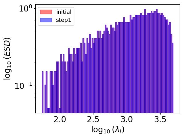
(a) GD $\eta=0.1$

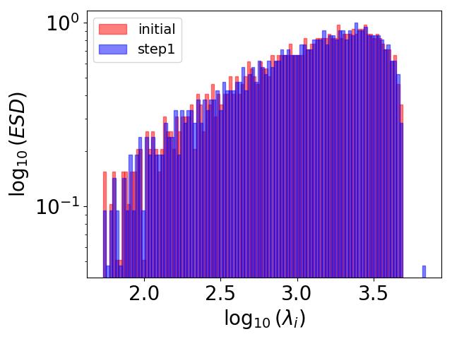
(b) GD $\eta=2000$

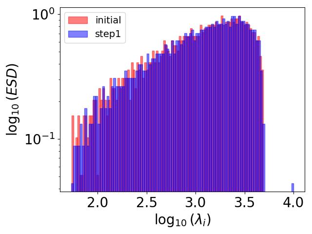
(c) FB-Adam $\eta=0.1$

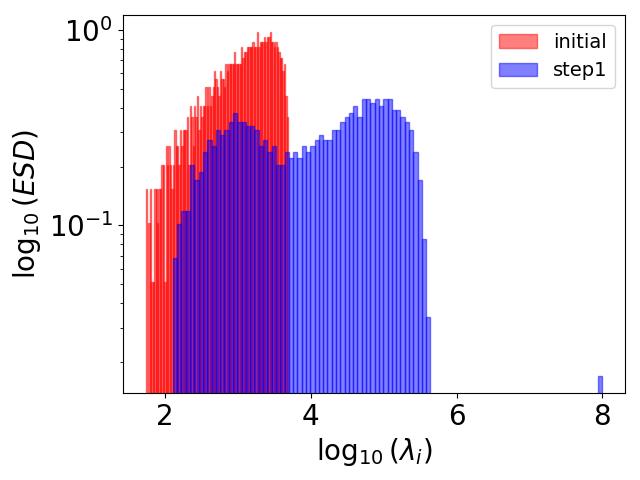
(d) FB-Adam $\eta=10$

Figure 2: Evolution of ESD of ${\mathbf{W}}^{\top}{\mathbf{W}}$ after one step optimizer update with varying learning rates. Here $n=2000$, $d=1000$, $h=1500$, $\sigma_{*}=\texttt{softplus},\sigma=\texttt{tanh},\rho_{e}=0.3$.

FB-Adam needs a much smaller learning rate than GD to have a spiked spectrum.

By varying the learning rate $\eta$, we train the student network $f(\cdot)$ for one step using GD and FB-Adam. We can observe from Figure 2(a) that after one GD update with $\eta=0.1$, the ESD of ${\mathbf{W}}_{1}^{\top}{\mathbf{W}}_{1}$ remains largely unchanged from that of ${\mathbf{W}}_{0}^{\top}{\mathbf{W}}_{0}$ (i.e ESD at initialization). On the other hand, Figure 2(b) illustrates that for $\eta=2000$, the ESD of ${\mathbf{W}}_{1}^{\top}{\mathbf{W}}_{1}$ exhibits a spike. However, this scaling does not hold for FB-Adam as the ESD of ${\mathbf{W}}_{1}^{\top}{\mathbf{W}}_{1}$ exhibits a spike after the first step even with a small learning rate of $\eta=0.1$ (see Figure 2(c)). Finally, for one step of FB-Adam with $\eta=10$, the ESD tends towards a seemingly bimodal distribution (see Figure 2(d)).

Impact of $\eta$ on losses, KTA, and sim$({\mathbf{W}},\beta*)$.

Since the choice of the optimizer affects the scale of the learning rate $\eta$ leading to a spike in the ESD of ${\mathbf{W}}_{1}^{\top}{\mathbf{W}}_{1}$, we vary $\eta$ across $\{0.001,0.01,0.1,1,10,100,1000,2000,3000\}$ and plot the means and standard deviations of losses, KTA and sim$({\mathbf{W}},\beta*)$ across $5$ runs in Figure 3. In the case of GD, observe that $\eta=2000$ is the threshold for the reduction of train and test losses (Figure 3(a)), an increase in KTA (Figure 3(c)), and an increase in sim$({\mathbf{W}},\beta*)$ (Figure 3(d)). Thus, implying that the occurrence of a spike leads to better generalization after one step. Similar observations for GD have been made in the mean-field setting by [27]. In the case of FB-Adam, we observe that $\eta=0.1$ is the threshold for an increase in KTA and sim$({\mathbf{W}},\beta*)$. However, for $\eta>1$, the training loss reduces considerably while the test loss increases. This shift is captured by a reversal of trend in the KTA plot. These observations hint at a sweet spot for $\eta$ beyond which FB-Adam leads to poor test performance. As a first step towards understanding these observations, we focus on the following pressing question: why does $\eta=0.1$ suffice for one-step of FB-Adam to exhibit a spike in the ESD of ${\mathbf{W}}_{1}^{\top}{\mathbf{W}}_{1}$, whereas one-step GD requires $\eta=2000$? Specifically, how large should $\eta$ be for FB-Adam to exhibit a spike in the ESD of ${\mathbf{W}}_{1}^{\top}{\mathbf{W}}_{1}$?

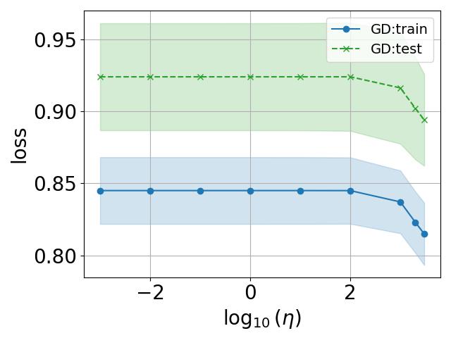
(a) GD loss

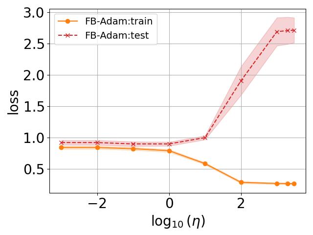
(b) FB-Adam loss

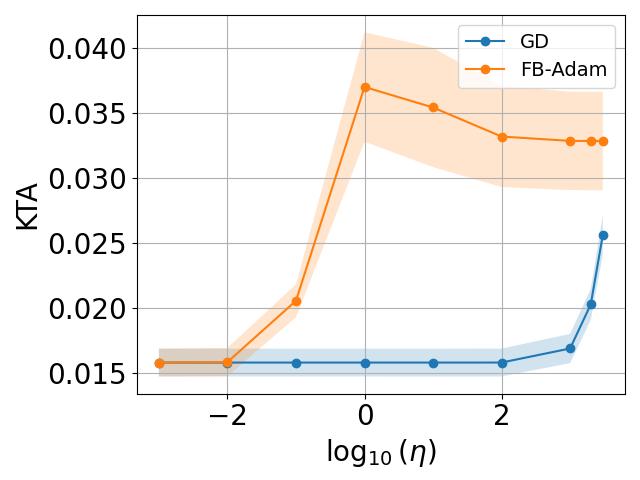
(c) KTA

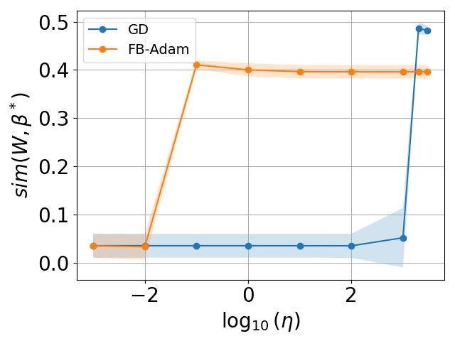
(d) sim$({\mathbf{W}},\beta*)$

Figure 3: Losses, KTA, sim$({\mathbf{W}},\beta*)$ for $f(\cdot)$ trained with one-step of GD, FB-Adam. Here $n=2000$, $d=1000$, $h=1500$, $\sigma_{*}=\texttt{softplus},\sigma=\texttt{tanh},\rho_{e}=0.3,\lambda=0.01$.

4.2 Theoretical Result of Learning Rate Scale for FB-Adam

To theoretically answer the above questions, we formulate the first step full batch gradient ${\mathbf{G}}_{0}$ as: G_0 &= 1nd [ 1h(ay^⊤-1h aa^⊤σ(1dW_0X^⊤) ) ⊙σ’(1dXW_0^⊤) ]X. Here $\sigma^{\prime}(\cdot):{\mathbb{R}}\to{\mathbb{R}}$ is the derivative of the activation function $\sigma$ acting element-wise on ${\mathbf{X}}{\mathbf{W}}_{0}^{\top}/\sqrt{d}$. Based on equation 3.1, let $\widetilde{{\mathbf{P}}}_{1}=\widetilde{{\mathbf{V}}}_{1}^{\circ 1/2}+\epsilon{\mathbf{1}}_{h\times d}$. Considering the FB-Adam epsilon hyper-parameter $\epsilon\approx 0$ [15], the update can be given as:

$$\widetilde{{\mathbf{G}}}_{0}=\widetilde{{\mathbf{P}}}_{1}^{\circ-1}\odot\widetilde{{\mathbf{M}}}_{1}=\frac{1-\beta_{1}}{\sqrt{1-\beta_{2}}}\operatorname{sign}({\mathbf{G}}_{0}).$$ (2)

Theorem 4.1.

Given the two-stage training procedure with large $n,d$, such that $n\asymp d$, and large (fixed) $h$, assume the teacher $F^{*}$ is $\lambda_{\sigma}$-Lipschitz with $\left\|F^{*}\right\|_{L^{2}}=\Theta_{d}(1)$, and a normalized ‘student’ activation $\sigma$, which has $\lambda_{\sigma}$-bounded first three derivatives almost surely and satisfies $\mathbb{E}[\sigma(z)]=0,\mathbb{E}[z\sigma(z)]\neq 0$, for $z\sim\mathcal{N}(0,1)$; then the matrix norm bounds for the one-step FB-Adam update can be given as:

$$\left\lVert\widetilde{{\mathbf{G}}}_{0}\right\rVert_{2}=\Theta_{d,\mathbb{P}}(\sqrt{hd}),\hskip 10.0pt\left\lVert\widetilde{{\mathbf{G}}}_{0}\right\rVert_{F}=\Theta_{d,\mathbb{P}}(\sqrt{hd}).$$ (3)

Appendix B presents the proof. The sketch of the proof is as follows: First, we show that ${\mathbf{G}}_{0}$ does not contain values that are exactly equal to $0$ almost surely. This allows us to obtain $\left\lVert\widetilde{{\mathbf{G}}}_{0}\right\rVert_{F}=\Theta_{d,\mathbb{P}}(\sqrt{hd})$. Next, we leverage a rank $1$ approximation ${\mathbf{A}}$ of ${\mathbf{G}}_{0}$ (in the operator norm [27]) to show that $\operatorname{sign}({\mathbf{A}})=\operatorname{sign}({\mathbf{G}}_{0})$. Finally, we obtain the lower-bound of $\left\lVert\widetilde{{\mathbf{G}}}_{0}\right\rVert_{2}=\Omega_{d,\mathbb{P}}(\sqrt{hd})$ to prove the theorem . The implications of this result are as follows.

Corollary 4.2.

Under the assumptions of Theorem 4.1, we have the following learning rate scales η= Θ(1) W_1 - W_0_F ≍W_0_F
η= Θ(1/h) W_1 - W_0_2 ≍W_0_2, where $\left\lVert{\mathbf{W}}_{0}\right\rVert_{2}=\Theta_{d,{\mathbb{P}}}(\sqrt{d}),\left\lVert{\mathbf{W}}_{0}\right\rVert_{F}=\Theta_{d,{\mathbb{P}}}(\sqrt{hd})$.

Discussion.

Intuitively, the essence of scaling the learning rate is as follows: choose $\eta$ such that $\eta\widetilde{{\mathbf{G}}}_{0}$ overwhelms ${\mathbf{W}}_{0}$ and results in feature learning for student network $f$. In the case of FB-Adam, observe that the Frobenius norm of $\widetilde{{\mathbf{G}}}_{0}$ is already quite large and is of the same order as ${\mathbf{W}}_{0}$. This indicates that $\eta=\Theta(1)$ is (sufficiently) large for the optimizer update to overwhelm the weights, and explains why a small learning rate $\eta=0.1$ suffices for the spikes in Figure 2 for FB-Adam. This also implies that: to prevent feature learning in the case of FB-Adam, we need to scale down the learning rate to an order of $\Theta(1/\sqrt{h})$. Note that our initialization strategy differs from the mean-field-based strategy of [27]. Appendix LABEL:app:mean_field_discussion discusses the scaling results for such a setup.

5 Singular Vector Alignments of Weights and Optimizer Updates

In this section, we leverage the scaling of learning rates to analyze the emergence of HT spectra in ${\mathbf{W}}$ after multiple update steps. By considering a common ‘update’ matrix ${\mathbf{M}}_{t}\in{\mathbb{R}}^{h\times d}$ , we denote the updates to hidden layer weight matrix ${\mathbf{W}}_{t}$ as follows: W_t+1 = W_t + M_t, where ${\mathbf{M}}_{t}$ is the optimizer update matrix based on GD (${\mathbf{M}}_{t}=-\eta{\mathbf{G}}_{t})$ or FB-Adam (${\mathbf{M}}_{t}=-\eta\widetilde{{\mathbf{G}}}_{t})$. By abstracting ${\mathbf{W}}_{t+1}$ as the ‘observation’, ${\mathbf{W}}_{t}$ as the ‘noise’ and ${\mathbf{M}}_{t}$ as the ‘signal’ rectangular matrices, we leverage methods from the rich literature on signal recovery in spiked matrix models [67, 68, 39, 38, 37, 69, 70, 71, 72, 73] to analyze the role of singular values and vectors of ${\mathbf{M}}_{t}$ in transforming the ESD of ${\mathbf{W}}_{t}^{\top}{\mathbf{W}}_{t}$ into a HT variant in ${\mathbf{W}}_{t+1}^{\top}{\mathbf{W}}_{t+1}$. Let $b=\min(h,d)$, we consider the SVD of ${\mathbf{W}}_{t+1},{\mathbf{W}}_{t},{\mathbf{M}}_{t}$ as: W_t+1 = U_W_t+1S_W_t+1V_W_t+1^⊤,     W_t = U_W_tS_W_tV_W_t^⊤,     M_t = U_M_tS_M_tV_M_t^⊤, where ${\mathbf{U}}_{W_{t+1}},{\mathbf{U}}_{W_{t}},{\mathbf{U}}_{M_{t}}\in{\mathbb{R}}^{h\times b}$, ${\mathbf{S}}_{W_{t+1}},{\mathbf{S}}_{W_{t}},{\mathbf{S}}_{M_{t}}\in{\mathbb{R}}^{b\times b}$ and ${\mathbf{V}}_{W_{t+1}},{\mathbf{V}}_{W_{t}},{\mathbf{V}}_{M_{t}}\in{\mathbb{R}}^{b\times d}$.

5.1 Alignment of Singular Vectors after One-Step Update

We begin our analysis with the first step update. Observe that ${\mathbf{W}}_{0}$ (at initialization) is a rectangular random Gaussian matrix, and the first step update ${\mathbf{M}}_{0}$ contains the signal obtained from backpropagation. From a signal recovery perspective, one can treat the scaling of the learning rates as amplifying the strength of the signal ${\mathbf{M}}_{0}$, such that it can be recovered from the observation ${\mathbf{W}}_{1}$.

Measuring alignments.

From the finite rank spiked matrix model, we know that the singular values ${\mathbf{S}}_{W_{1}}$ are non-linear transformations (also termed as ‘inflations’ [37]) of ${\mathbf{S}}_{M_{0}}$, and ${\mathbf{U}}_{W_{1}},{\mathbf{V}}_{W_{1}}$ are rotated variants of ${\mathbf{U}}_{M_{0}},{\mathbf{V}}_{M_{0}}$ respectively. Formally, let $\hat{s}_{1}\geq\hat{s}_{2}\cdots\geq\hat{s}_{b}$ denote the singular values of ${\mathbf{W}}_{1}$, and let $s_{1}\geq s_{2}\cdots\geq s_{b}$ denote the singular values of ${\mathbf{M}}_{0}$. Let $\hat{{\mathbf{u}}}_{j}\in{\mathbb{R}}^{h},\hat{{\mathbf{v}}}_{j}\in{\mathbb{R}}^{d}$ represent the left and right singular vectors of ${\mathbf{W}}_{1}$ corresponding to singular value $\hat{s}_{j}$. Similarly, let ${\mathbf{u}}_{k}\in{\mathbb{R}}^{h},{\mathbf{v}}_{k}\in{\mathbb{R}}^{d}$ represent the left and right singular vectors of ${\mathbf{M}}_{0}$ corresponding to singular value $s_{k}$. Owing to the rotational invariant nature of the Gaussian matrix ${\mathbf{W}}_{0}$, the alignment values $\mathbb{E}\left[(\hat{{\mathbf{u}}}_{j}^{\top}{\mathbf{u}}_{k})^{2}\right],\mathbb{E}\left[(\hat{{\mathbf{v}}}_{j}^{\top}{\mathbf{v}}_{k})^{2}\right],\forall j,k\in\{1,\cdots,b\}$ can be computed solely based on $\hat{s}_{j},s_{k}$ (see [37] and [74]). Empirically, we measure these collective alignments using the ‘overlaps’ between two singular vector matrices as follows:

Definition 5.1.

The ‘overlaps’ between two singular vector matrices ${\mathbf{J}},{\mathbf{Q}}\in{\mathbb{R}}^{a\times b}$ is defined as: O(J, Q) = (J^⊤Q)^∘2 ∈R^b ×b

Overlaps after one-step.

Using the experimental setup described in Section 4 for one-step update, we compute: ${\mathcal{O}}({\mathbf{U}}_{W_{0}},{\mathbf{U}}_{M_{0}}),{\mathcal{O}}({\mathbf{V}}_{W_{0}},{\mathbf{V}}_{M_{0}}),{\mathcal{O}}({\mathbf{U}}_{W_{1}},{\mathbf{U}}_{M_{0}}),{\mathcal{O}}({\mathbf{V}}_{W_{1}},{\mathbf{V}}_{M_{0}})$. The key observation is that scaling of learning rates leads to larger alignments between singular vectors. In the case of FB-Adam with $\eta=1$, ${\mathbf{W}}_{0}$ is a random Gaussian and the overlaps ${\mathcal{O}}({\mathbf{U}}_{W_{0}},{\mathbf{U}}_{M_{0}}),{\mathcal{O}}({\mathbf{V}}_{W_{0}},{\mathbf{V}}_{M_{0}})$ do not exhibit any significant outliers even for large $\eta$ (see Figure 4(a), 4(b)). However, the overlaps ${\mathcal{O}}({\mathbf{U}}_{W_{1}},{\mathbf{U}}_{M_{0}}),{\mathcal{O}}({\mathbf{V}}_{W_{1}},{\mathbf{V}}_{M_{0}})$ in Figure 4(c), 4(d) are representative of the spike in the ESD. Similar observations can be made for GD($\eta=2000$) (Appendix LABEL:app:add_exp).

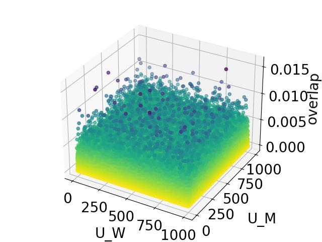
(a) ${\mathcal{O}}({\mathbf{U}}_{W_{0}},{\mathbf{U}}_{M_{0}})$

(b) ${\mathcal{O}}({\mathbf{V}}_{W_{0}},{\mathbf{V}}_{M_{0}})$

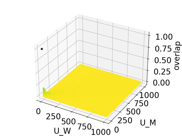
(c) ${\mathcal{O}}({\mathbf{U}}_{W_{1}},{\mathbf{U}}_{M_{0}})$

(d) ${\mathcal{O}}({\mathbf{V}}_{W_{1}},{\mathbf{V}}_{M_{0}})$

Figure 4: Overlaps between singular vectors after one step of FB-Adam($\eta=1$).

5.2 Heavy-Tailed Phenomenon after Multiple Steps

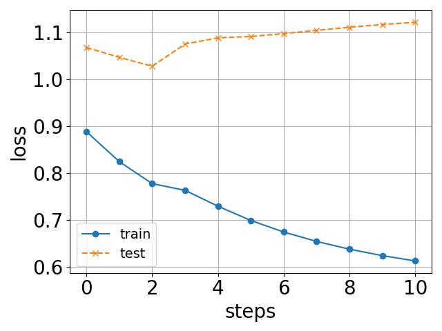
(a) losses

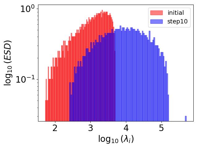
(b) ESD of ${\mathbf{W}}^{\top}{\mathbf{W}}$

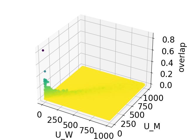
(c) ${\mathcal{O}}({\mathbf{U}}_{W_{10}},{\mathbf{U}}_{M_{9}})$

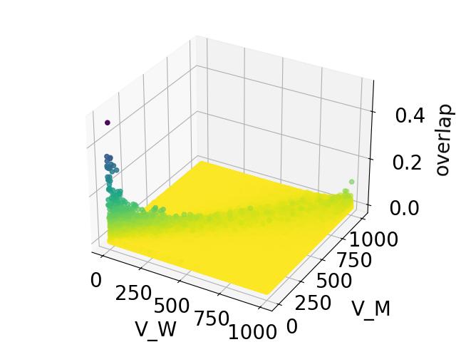
(d) ${\mathcal{O}}({\mathbf{V}}_{W_{10}},{\mathbf{V}}_{M_{9}})$

Figure 5: Train/test losses, ESD of ${\mathbf{W}}^{\top}{\mathbf{W}}$, and Overlaps between singular vectors ${\mathcal{O}}({\mathbf{U}}_{W_{10}},{\mathbf{U}}_{M_{9}})$, ${\mathcal{O}}({\mathbf{V}}_{W_{10}},{\mathbf{V}}_{M_{9}})$ for $f(\cdot)$ trained with $10$ steps of FB-Adam($\eta=1$).

After multiple optimizer updates, the weight matrix ${\mathbf{W}}_{t},\forall t>1$ no longer has i.i.d. entries. In particular, it accumulates the signal from previous update steps. Using the experimental setup described in Section 4 for one-step update, we apply $10$ optimizer updates to obtain: ${\mathbf{W}}_{10}={\mathbf{W}}_{9}+{\mathbf{M}}_{9}$ and compute: ${\mathcal{O}}({\mathbf{U}}_{W_{10}},{\mathbf{U}}_{M_{9}}),{\mathcal{O}}({\mathbf{V}}_{W_{10}},{\mathbf{V}}_{M_{9}})$.

In the case of FB-Adam($\eta=1$), the ESD of ${\mathbf{W}}_{10}^{\top}{\mathbf{W}}_{10}$ (Figure 5(b)) tends to exhibits a heavier tail distribution (which is relatively heavier than GD($\eta=2000$), see Figure LABEL:fig:app:10_step_gd_lr2000_W_esd in Appendix LABEL:app:add_exp). Next, observe that ${\mathcal{O}}({\mathbf{V}}_{W_{10}},{\mathbf{V}}_{M_{9}})$ (in Figure 5(d)) fails to exhibit high (outlier) alignment values relative to the one-step update case (in Figure 4(d)). Finally, we make a surprising observation that the overlaps ${\mathcal{O}}({\mathbf{U}}_{W_{10}},{\mathbf{U}}_{M_{9}}),{\mathcal{O}}({\mathbf{V}}_{W_{10}},{\mathbf{V}}_{M_{9}})$ in Figure 5(c), 5(d) seems to exhibit a heavy-tail like distribution along the diagonal.

Weight normalization (WN) facilitates heavier-tailed spectra.

We employ a simple weight normalization technique [75] after each optimizer update to ${\mathbf{W}}$ as follows: W_t+1 = hdWt+1’Wt+1’F,    W_t+1’ = W_t + M_t. This step ensures that $\left\lVert{\mathbf{W}}_{t+1}\right\rVert_{F}$ is always $\sqrt{hd}$, before the forward pass. We observe that this approach leads to a wider ESD of ${\mathbf{W}}_{10}^{\top}{\mathbf{W}}_{10}$ (in Figure 6(b)) when compared to its un-normalized counterpart in Figure 5(b). Additionally, the overlap values ${\mathcal{O}}({\mathbf{U}}_{W_{10}},{\mathbf{U}}_{M_{9}}),{\mathcal{O}}({\mathbf{V}}_{W_{10}},{\mathbf{V}}_{M_{9}})$ in Figure 6(c), 6(d) have a wider spread on the off-diagonal entries than the un-normalized case in Figure 5(c), 5(d). The relationship between the distribution of the overlap values along the diagonal and off-diagonal and the heaviness of the ESD tail requires a separate in-depth analysis. To this end, we defer such quantification studies to future work.

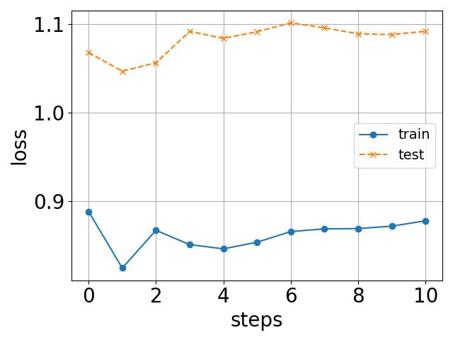
(a) losses

(b) ESD ${\mathbf{W}}^{\top}{\mathbf{W}}$

(c) ${\mathcal{O}}({\mathbf{U}}_{W_{10}},{\mathbf{U}}_{M_{9}})$

(d) ${\mathcal{O}}({\mathbf{V}}_{W_{10}},{\mathbf{V}}_{M_{9}})$

Figure 6: Train/test losses, ESD of ${\mathbf{W}}^{\top}{\mathbf{W}}$, and Overlaps between singular vectors ${\mathcal{O}}({\mathbf{U}}_{W_{10}},{\mathbf{U}}_{M_{9}})$, ${\mathcal{O}}({\mathbf{V}}_{W_{10}},{\mathbf{V}}_{M_{9}})$ for $f(\cdot)$ trained with $10$ steps of FB-Adam($\eta=1$) with weight normalization.

5.3 Impact on Generalization after Multiple Steps

In this section, we analyze the conditions under which a heavy-tailed spectrum of ${\mathbf{W}}^{\top}{\mathbf{W}}$ can lead to better/worse training and test loss after multiple GD/FB-Adam updates.

Setup.

We consider the two-layer student NN $f(\cdot)$ of width $h=1500,\sigma=\texttt{tanh}$ and train it on a dataset of size $n=8000$ for $10$ steps using GD/FB-Adam. We choose a sample dimension $d=1000$, $\sigma_{*}=\texttt{softplus}$ and $\rho_{e}=0.3$. The test dataset has $200$ samples.

Correlations between ESD and losses.

We plot the means and standard deviations across $5$ runs for the train/test losses, KTA, PL_Alpha_Hill and PL_Alpha_KS of ${\mathbf{W}}_{10}^{\top}{\mathbf{W}}_{10}$ after $10$ GD/FB-Adam updates by varying $\eta$ across $\{0.001,0.01,0.1,1,10,100,1000,2000,3000\}$ in Figure 7. Here PL_Alpha_Hill [6], PL_Alpha_KS refer to the power-law (PL) exponents that are fit to the ESD of ${\mathbf{W}}_{t}^{\top}{\mathbf{W}}_{t}$ using the Hill estimator [76] and based on the Kolmogorov–Smirnoff statistic respectively [4, 2, 77]. A lower value of PL_Alpha_Hill / PL_Alpha_KS indicates a heavier-tailed spectrum.

First, observe that for GD with $\eta\geq 1000$, the reduction in train and test losses are correlated with an increase in KTA and a decrease in PL_Alpha_Hill and PL_Alpha_KS to an extent. In the case of FB-Adam, a similar correlation between the training loss, KTA, PL_Alpha_Hill and PL_Alpha_KS can be observed. However, there seems to be a region of benign learning rates ($\eta\leq 1$) for which a decrease in PL_Alpha_Hill leads to better test performance. For $1\leq\eta\leq 100$, although we observe similar values of PL_Alpha_Hill, the ESDs of ${\mathbf{W}}_{10}^{\top}{\mathbf{W}}_{10}$ differ in the scale of the singular values, and the spike seems to have a large influence on the estimation of PL_Alpha_Hill (see Figure LABEL:fig:app:10_step_fb_adam_W_esd_n_8000_eta_1_to_1000 in Appendix LABEL:app:add_exp). However, the PL_Alpha_KS captures the monotonically decreasing trend for this range of $\eta$. A similar analysis with weight normalization is presented in Figure LABEL:fig:gd_fb_adam_bulk_loss_alignments_10_steps_n_8000_wn in Appendix LABEL:app:add_exp.

(a) loss

(b) KTA

(c) PL_Alpha_Hill

(d) PL_Alpha_KS

Figure 7: Losses, KTA, PL_Alpha_Hill, PL_Alpha_KS for $f(\cdot)$ trained with $10$ steps of GD, FB-Adam, with $n=8000$, $d=1000$, $h=1500$, $\sigma_{*}=\texttt{softplus},\sigma=\texttt{tanh},\rho_{e}=0.3,\lambda=0.01$.

Role of sample size ($n$).

By fixing $d=1000,h=1500$ and $\eta=1$, we vary the size of the training dataset $n$ as per the set $\{500,2000,4000,8000\}$. In this setting, observe from Figure 8(a) that the train loss and test loss improve significantly for $n=8000$, while the network overfits for smaller $n$. Furthermore, for $n=2000$, we observed that ${\mathbf{W}}_{10}^{\top}{\mathbf{W}}_{10}$ exhibits a heavy-tailed ESD with PL_Alpha_Hill$=1.8$ (Figure LABEL:fig:app:gd_fb_adam_bulk_loss_alignments_10_steps_n_2000_alpha), which is less than the $n=8000$ case of $\approx 1.9$ (see Figure 7(c)). The key difference in the latter case is that the spike in the ESD is consumed by the bulk, unlike the former where the outlier singular value is almost an order of magnitude away from the bulk.

Role of regularization constant ($\lambda$).

By considering a sample size of $n=8000$, and fixing $d=1000,h=1500,\eta=1$ as before, we can observe from Figure 8(b) that a lower training and test loss is achieved by $\lambda=10^{-3}$ and $\lambda=10^{-4}$, but with a large generalization gap (i.e. the difference between train and test loss). Additionally, observe that $\lambda=10^{-2}$ reasonably balances the test loss and generalization gap. Since the regression procedure does not modify the first layer weights, the choice of $\lambda$ can affect the interpretation of heavy tails leading to good/bad generalization.

Role of label noise ($\rho_{e}$).

Figure 8(c) illustrates a consistent increase in losses for an increase in the additive Gaussian label noise $\rho_{e}$ from $\{0.1,0.3,0.5,0.7\}$. However, the ESD of ${\mathbf{W}}_{10}^{\top}{\mathbf{W}}_{10}$ alone does not provide the complete picture to reflect this difficulty in learning. Instead, we observe noticeable differences in the distribution of values (especially outliers) along the diagonal of overlap matrices ${\mathcal{O}}({\mathbf{U}}_{W_{10}},{\mathbf{U}}_{M_{9}})$, ${\mathcal{O}}({\mathbf{V}}_{W_{10}},{\mathbf{V}}_{M_{9}})$ for $\rho_{e}=0.3$ (Figure LABEL:fig:app:overlap_fb_adam_lr1_n_8000_u_o10, LABEL:fig:app:overlap_fb_adam_lr1_n_8000_v_o10) and $\rho_{e}=0.7$ (Figure LABEL:fig:app:overlap_fb_adam_lr1_n_8000_rho_0.7_u_o10, LABEL:fig:app:overlap_fb_adam_lr1_n_8000_rho_0.7_v_o10). Especially, the outliers in the former case had smaller values (almost $0.5\times$) than the latter.

Role of learning rate scheduling.

Finally, as a natural extension of selecting a large learning rate at initialization, we analyze the role of employing learning rate schedules [59, 78, 79, 80] on the losses and ESD of ${\mathbf{W}}^{\top}{\mathbf{W}}$. We consider the simple torch.optim.StepLR scheduler with varying decay factors ($\gamma$) per step. A smaller $\gamma$ indicates a faster decay in the learning rate $\eta$ per step. We observe from Figure 8(d) that such fast decays (with $\gamma=0.2$ and $\gamma=0.4$) quickly turns a large learning rate to a smaller one and lead to stable loss curves. However, the trends are relatively unstable for $\gamma=0.6$ and $\gamma=0.8$ in the early steps. Finally, by employing WN, we can control the presence of the spike while nudging the bulk of the ESD toward an HT distribution with such schedules (Figure LABEL:fig:app:10_step_gd_fb_adam_W_esd_steplr).

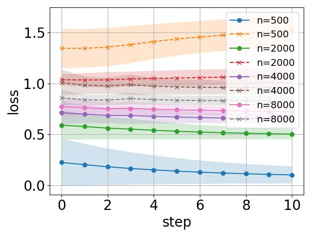
(a) vary $n$

(b) vary $\lambda$

(c) vary $\rho_{e}$

(d) vary StepLR ($\gamma$)

Figure 8: FB-Adam train/test loss across $10$ steps with varying $n,\lambda,\rho_{e}$ and StepLR($\gamma$). (a) Varying dataset size $n$ (b) Varying regularization parameter $\lambda$ for obtaining the second-layer weights, (c) Varying the std.dev ($\rho_{e}$) of the additive Gaussian label noise, (d) Varying the StepLR($\gamma$) parameter which controls the decay of $\eta$. The bold lines indicate train loss and the dashed lines indicate test loss.

6 Conclusion

This paper presents a different angle in the study of the emergence of HT spectra in NN training. Unlike existing explanations using stochastic gradient noise, we show that full-batch GD or Adam can still lead to HT ESDs in the weight matrices after only a few optimizer updates. The HT ESDs arise from the interactions between the signal (the gradient update) and the noise (the initial Marchenko–Pastur bulk), and they only occur when the learning rate is sufficiently large. In addition to being a new way of explaining the emergence of HT ESDs, our paper connects with several ongoing studies in this field. First, our study analyzes the "bulk-decay" type of ESDs in the "5+1" phase model [3], which is the crucial connection between classical "bulk+spike" ESDs and HT ESD models. Our paper views the "bulk-decay" ESD as an intermediate state generated from diffusing the spike into the main bulk (Appendix  LABEL:spike_movement). Second, our study tightens the connection between ESDs and feature learning, explaining why ESD-based training methods [6] can improve the generalizability of large and deep models. Our paper also presents several surprising phenomena: (1) the emergence of the HT spectra seems to require only a single spike aligned with the teacher model; (2) the emergence of the HT spectra can appear early during training, way before the NN reaches a low training loss; (3) several factors, such as weight normalization and learning rate scheduling, can all contribute to the emergence of HT ESDs.

Future work.

By presenting qualitative results that indicate heavy tails along the diagonals of overlap matrices, we aim to bring singular vectors into the picture for future heavy-tail studies. Particularly, how does the distribution of values along the diagonal change for overlap matrices of left and right singular vectors? How do we quantify the ‘spread’ of the off-diagonal overlap values? Furthermore, several papers have studied how to rigorously characterize the loss after a one-step GD update [56, 36], and an interesting direction is to explore the relationship between ESD of ${\mathbf{W}}_{t}^{\top}{\mathbf{W}}_{t}$ and theoretical loss after $t$ optimizer updates (for GD/FB-Adam).

Acknowledgements.

The authors would like to thank Zhichao Wang for helpful discussions during the preparation of the manuscript.

Appendix A Generating Very Heavy-Tailed Spectra without Gradient Noise

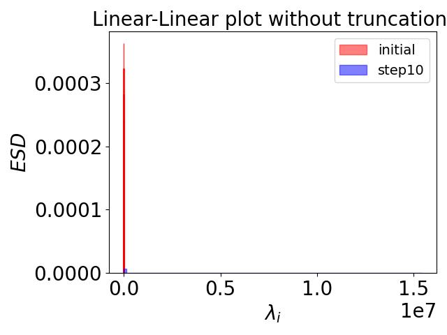
(a) GD $\eta=5000$

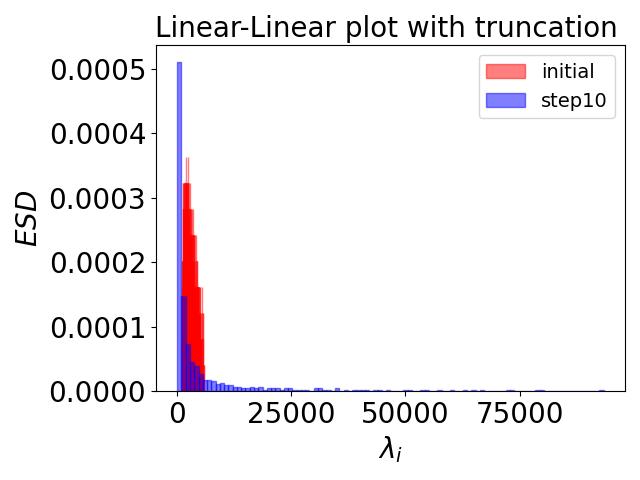
(b) GD $\eta=5000$

(c) GD $\eta=5000$

(d) FB-Adam $\eta=3$

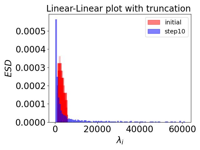
(e) FB-Adam $\eta=3$

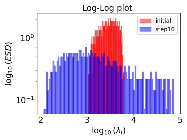
(f) FB-Adam $\eta=3$

Figure 9: Emergence of HT spectra after 10 GD/FB-Adam steps with weight normalization. Here $n=4000$, $d=500$, $h=3000$, $\sigma_{*}=\texttt{softplus},\sigma=\texttt{tanh},\rho_{e}=0.3$. PL_Alpha_KS for GD (first row) is 1.58, and PL_Alpha_KS for FB-Adam (second row) is 1.59.

In this section, we present two examples of highly HT spectra, shown in Figure 9. If one only observes the linear-linear plot (first column), the shapes can be invisible due to large eigenvalues. For example, see Figure 9(a). After truncation, they become clearer (middle column). To quantitatively verify our observations, we adopted the WeightWatcher [2] Python APIs to fit a power-law (PL) distribution to these ESDs. We find that both ESDs have a PL coefficient PL_Alpha_KS smaller than 2. As discussed in [3, Table 3], this indicates that these ESDs have entered the very HT regime. More importantly, these ESDs are generated without gradient noise after only 10 GD/FB-Adam steps.

Appendix B Proof of Theorem 4.1

In this section, we prove Theorem 4.1, and conduct numerical simulations for empirical verification. We begin by stating and discussing the main assumptions of the theorem.

Assumption B.1.

Gaussian Initialization. The entries of the weights are sampled independently as $\left[{\mathbf{W}}_{0}\right]_{ij}\stackrel{{\scriptstyle\text{i.i.d.}}}{{\sim}}\mathcal{N}(0,1)$ and $\left[a\right]_{i}\stackrel{{\scriptstyle\text{i.i.d.}}}{{\sim}}\mathcal{N}(0,1),\forall i\in[h],j\in[d]$.

Assumption B.2.

Normalized Activation. The nonlinear activation $\sigma$ has $\lambda_{\sigma}$-bounded first three derivatives almost surely. In addition, $\sigma$ satisfies $\mathbb{E}[\sigma(z)]=0,\mathbb{E}[z\sigma(z)]\neq 0$, for $z\sim\mathcal{N}(0,1)$.

Discussion. Consider $\sigma:{\mathbb{R}}\to{\mathbb{R}}$ to be the tanh function and $z\sim\mathcal{N}(0,1)$. Since $\sigma(z)=\texttt{tanh}(z)=\frac{e^{z}-e^{-z}}{e^{z}+e^{-z}}$, it is easy to check that $\sigma(z)$ has $1-$bounded first three derivatives and it is an odd function satisfying $\sigma(z)=-\sigma(-z)$, we have: E_p(z)[σ(z)]&=∫_-∞

References

- [1] Charles H Martin and Michael W Mahoney. Heavy-tailed universality predicts trends in test accuracies for very large pre-trained deep neural networks. In Proceedings of the 2020 SIAM International Conference on Data Mining, pages 505–513. SIAM, 2020.
- [2] Charles H Martin, Tongsu Peng, and Michael W Mahoney. Predicting trends in the quality of state-of-the-art neural networks without access to training or testing data. Nature Communications, 12(1):4122, 2021.
- [3] Charles H Martin and Michael W Mahoney. Implicit self-regularization in deep neural networks: Evidence from random matrix theory and implications for learning. The Journal of Machine Learning Research, 22(1):7479–7551, 2021.
- [4] Yaoqing Yang, Ryan Theisen, Liam Hodgkinson, Joseph E Gonzalez, Kannan Ramchandran, Charles H Martin, and Michael W Mahoney. Test accuracy vs. generalization gap: Model selection in nlp without accessing training or testing data. In Proceedings of the 29th ACM SIGKDD Conference on Knowledge Discovery and Data Mining, pages 3011–3021, 2023.
- [5] Zhichao Wang, Andrew William Engel, Anand Sarwate, Ioana Dumitriu, and Tony Chiang. Spectral evolution and invariance in linear-width neural networks. In Thirty-seventh Conference on Neural Information Processing Systems, 2023.
- [6] Yefan Zhou, Tianyu Pang, Keqin Liu, Charles H. Martin, Michael W. Mahoney, and Yaoqing Yang. Temperature balancing, layer-wise weight analysis, and neural network training. In Thirty-seventh Conference on Neural Information Processing Systems, 2023.
- [7] Mert Gurbuzbalaban, Umut Simsekli, and Lingjiong Zhu. The heavy-tail phenomenon in sgd. In International Conference on Machine Learning, pages 3964–3975. PMLR, 2021.
- [8] Umut Simsekli, Levent Sagun, and Mert Gurbuzbalaban. A tail-index analysis of stochastic gradient noise in deep neural networks. In International Conference on Machine Learning, pages 5827–5837. PMLR, 2019.
- [9] Umut Simsekli, Ozan Sener, George Deligiannidis, and Murat A Erdogdu. Hausdorff dimension, heavy tails, and generalization in neural networks. Advances in Neural Information Processing Systems, 33:5138–5151, 2020.
- [10] Krunoslav Lehman Pavasovic, Alain Durmus, and Umut Simsekli. Approximate heavy tails in offline (multi-pass) stochastic gradient descent. arXiv preprint arXiv:2310.18455, 2023.
- [11] Liam Hodgkinson and Michael Mahoney. Multiplicative noise and heavy tails in stochastic optimization. In International Conference on Machine Learning, pages 4262–4274. PMLR, 2021.
- [12] Anant Raj, Lingjiong Zhu, Mert Gurbuzbalaban, and Umut Simsekli. Algorithmic stability of heavy-tailed sgd with general loss functions. In International Conference on Machine Learning, pages 28578–28597. PMLR, 2023.
- [13] Liam Hodgkinson, Chris van der Heide, Robert Salomone, Fred Roosta, and Michael W Mahoney. The interpolating information criterion for overparameterized models. arXiv preprint arXiv:2307.07785, 2023.
- [14] Diederik P Kingma and Jimmy Ba. Adam: A method for stochastic optimization. arXiv preprint arXiv:1412.6980, 2014.
- [15] Frederik Kunstner, Jacques Chen, Jonathan Wilder Lavington, and Mark Schmidt. Noise is not the main factor behind the gap between sgd and adam on transformers, but sign descent might be. In The Eleventh International Conference on Learning Representations, 2022.
- [16] Sebastian Goldt, Madhu Advani, Andrew M Saxe, Florent Krzakala, and Lenka Zdeborová. Dynamics of stochastic gradient descent for two-layer neural networks in the teacher-student setup. Advances in neural information processing systems, 32, 2019.
- [17] Gerard Ben Arous, Reza Gheissari, and Aukosh Jagannath. Online stochastic gradient descent on non-convex losses from high-dimensional inference. Journal of Machine Learning Research, 22(106):1–51, 2021.
- [18] Jean Barbier, Florent Krzakala, Nicolas Macris, Léo Miolane, and Lenka Zdeborová. Optimal errors and phase transitions in high-dimensional generalized linear models. Proceedings of the National Academy of Sciences, 116(12):5451–5460, 2019.
- [19] Marco Mondelli and Andrea Montanari. Fundamental limits of weak recovery with applications to phase retrieval. In Conference On Learning Theory, pages 1445–1450. PMLR, 2018.
- [20] Antoine Maillard, Gérard Ben Arous, and Giulio Biroli. Landscape complexity for the empirical risk of generalized linear models. In Mathematical and Scientific Machine Learning, pages 287–327. PMLR, 2020.
- [21] Alberto Bietti, Joan Bruna, Clayton Sanford, and Min Jae Song. Learning single-index models with shallow neural networks. Advances in Neural Information Processing Systems, 35:9768–9783, 2022.
- [22] Alireza Mousavi-Hosseini, Sejun Park, Manuela Girotti, Ioannis Mitliagkas, and Murat A Erdogdu. Neural networks efficiently learn low-dimensional representations with sgd. In The Eleventh International Conference on Learning Representations, 2022.
- [23] Aaron Zweig, Loucas Pillaud-Vivien, and Joan Bruna. On single-index models beyond gaussian data. In Thirty-seventh Conference on Neural Information Processing Systems, 2023.
- [24] Jimmy Ba, Murat A Erdogdu, Taiji Suzuki, Zhichao Wang, and Denny Wu. Learning in the presence of low-dimensional structure: A spiked random matrix perspective. In Thirty-seventh Conference on Neural Information Processing Systems, 2023.
- [25] Alireza Mousavi-Hosseini, Denny Wu, Taiji Suzuki, and Murat A Erdogdu. Gradient-based feature learning under structured data. In Thirty-seventh Conference on Neural Information Processing Systems, 2023.
- [26] Alex Damian, Eshaan Nichani, Rong Ge, and Jason D Lee. Smoothing the landscape boosts the signal for sgd: Optimal sample complexity for learning single index models. In Thirty-seventh Conference on Neural Information Processing Systems, 2023.
- [27] Jimmy Ba, Murat A Erdogdu, Taiji Suzuki, Zhichao Wang, Denny Wu, and Greg Yang. High-dimensional asymptotics of feature learning: How one gradient step improves the representation. Advances in Neural Information Processing Systems, 35:37932–37946, 2022.
- [28] Yatin Dandi, Emanuele Troiani, Luca Arnaboldi, Luca Pesce, Lenka Zdeborová, and Florent Krzakala. The benefits of reusing batches for gradient descent in two-layer networks: Breaking the curse of information and leap exponents. arXiv preprint arXiv:2402.03220, 2024.
- [29] Peter McCullagh. Generalized linear models. Routledge, 2019.
- [30] Wolfgang Härdle, Marlene Müller, Stefan Sperlich, Axel Werwatz, et al. Nonparametric and semiparametric models, volume 1. Springer, 2004.
- [31] Surbhi Goel, Aravind Gollakota, Zhihan Jin, Sushrut Karmalkar, and Adam Klivans. Superpolynomial lower bounds for learning one-layer neural networks using gradient descent. In International Conference on Machine Learning, pages 3587–3596. PMLR, 2020.
- [32] Rishabh Dudeja and Daniel Hsu. Learning single-index models in gaussian space. In Conference On Learning Theory, pages 1887–1930. PMLR, 2018.
- [33] Sham M Kakade, Varun Kanade, Ohad Shamir, and Adam Kalai. Efficient learning of generalized linear and single index models with isotonic regression. Advances in Neural Information Processing Systems, 24, 2011.
- [34] Mahdi Soltanolkotabi. Learning relus via gradient descent. Advances in neural information processing systems, 30, 2017.
- [35] Yatin Dandi, Florent Krzakala, Bruno Loureiro, Luca Pesce, and Ludovic Stephan. How two-layer neural networks learn, one (giant) step at a time. In NeurIPS 2023 Workshop on Mathematics of Modern Machine Learning, 2023.
- [36] Hugo Cui, Luca Pesce, Yatin Dandi, Florent Krzakala, Yue M Lu, Lenka Zdeborová, and Bruno Loureiro. Asymptotics of feature learning in two-layer networks after one gradient-step. arXiv preprint arXiv:2402.04980, 2024.
- [37] Itamar D. Landau, Gabriel C. Mel, and Surya Ganguli. Singular vectors of sums of rectangular random matrices and optimal estimation of high-rank signals: The extensive spike model. Phys. Rev. E, 108:054129, Nov 2023.
- [38] Florent Benaych-Georges and Raj Rao Nadakuditi. The singular values and vectors of low rank perturbations of large rectangular random matrices. Journal of Multivariate Analysis, 111:120–135, 2012.
- [39] Andrey A Shabalin and Andrew B Nobel. Reconstruction of a low-rank matrix in the presence of gaussian noise. Journal of Multivariate Analysis, 118:67–76, 2013.
- [40] Jeffrey Pennington and Pratik Worah. Nonlinear random matrix theory for deep learning. Advances in neural information processing systems, 30, 2017.
- [41] Cosme Louart, Zhenyu Liao, and Romain Couillet. A random matrix approach to neural networks. The Annals of Applied Probability, 28(2):1190–1248, 2018.
- [42] Oussama Dhifallah and Yue M Lu. A precise performance analysis of learning with random features. arXiv preprint arXiv:2008.11904, 2020.
- [43] Federica Gerace, Bruno Loureiro, Florent Krzakala, Marc Mézard, and Lenka Zdeborová. Generalisation error in learning with random features and the hidden manifold model. In International Conference on Machine Learning, pages 3452–3462. PMLR, 2020.
- [44] Ben Adlam and Jeffrey Pennington. The neural tangent kernel in high dimensions: Triple descent and a multi-scale theory of generalization. In International Conference on Machine Learning, pages 74–84. PMLR, 2020.
- [45] Song Mei and Andrea Montanari. The generalization error of random features regression: Precise asymptotics and the double descent curve. Communications on Pure and Applied Mathematics, 75(4):667–766, 2022.
- [46] Yongqi Du, Di Xie, Shiliang Pu, Robert Qiu, Zhenyu Liao, et al. " lossless" compression of deep neural networks: A high-dimensional neural tangent kernel approach. Advances in Neural Information Processing Systems, 35:3774–3787, 2022.
- [47] Dominik Schröder, Hugo Cui, Daniil Dmitriev, and Bruno Loureiro. Deterministic equivalent and error universality of deep random features learning. In International Conference on Machine Learning, pages 30285–30320. PMLR, 2023.
- [48] Mei Song, Andrea Montanari, and P Nguyen. A mean field view of the landscape of two-layers neural networks. Proceedings of the National Academy of Sciences, 115(33):E7665–E7671, 2018.
- [49] Andrea Montanari and Basil N Saeed. Universality of empirical risk minimization. In Conference on Learning Theory, pages 4310–4312. PMLR, 2022.
- [50] Hong Hu and Yue M Lu. Universality laws for high-dimensional learning with random features. IEEE Transactions on Information Theory, 69(3):1932–1964, 2022.
- [51] Sebastian Goldt, Bruno Loureiro, Galen Reeves, Florent Krzakala, Marc Mézard, and Lenka Zdeborová. The gaussian equivalence of generative models for learning with shallow neural networks. In Mathematical and Scientific Machine Learning, pages 426–471. PMLR, 2022.
- [52] Yatin Dandi, Ludovic Stephan, Florent Krzakala, Bruno Loureiro, and Lenka Zdeborová. Universality laws for gaussian mixtures in generalized linear models. Advances in Neural Information Processing Systems, 36, 2024.
- [53] Bruno Loureiro, Cedric Gerbelot, Hugo Cui, Sebastian Goldt, Florent Krzakala, Marc Mezard, and Lenka Zdeborová. Learning curves of generic features maps for realistic datasets with a teacher-student model. Advances in Neural Information Processing Systems, 34:18137–18151, 2021.
- [54] Fanghui Liu, Zhenyu Liao, and Johan Suykens. Kernel regression in high dimensions: Refined analysis beyond double descent. In International Conference on Artificial Intelligence and Statistics, pages 649–657. PMLR, 2021.
- [55] Zhenyu Liao, Romain Couillet, and Michael W Mahoney. A random matrix analysis of random fourier features: beyond the gaussian kernel, a precise phase transition, and the corresponding double descent. Advances in Neural Information Processing Systems, 33:13939–13950, 2020.
- [56] Behrad Moniri, Donghwan Lee, Hamed Hassani, and Edgar Dobriban. A theory of non-linear feature learning with one gradient step in two-layer neural networks. arXiv preprint arXiv:2310.07891, 2023.
- [57] Maksym Andriushchenko, Aditya Vardhan Varre, Loucas Pillaud-Vivien, and Nicolas Flammarion. Sgd with large step sizes learns sparse features. In International Conference on Machine Learning, pages 903–925. PMLR, 2023.
- [58] Aitor Lewkowycz, Yasaman Bahri, Ethan Dyer, Jascha Sohl-Dickstein, and Guy Gur-Ari. The large learning rate phase of deep learning: the catapult mechanism. arXiv preprint arXiv:2003.02218, 2020.
- [59] Yuanzhi Li, Colin Wei, and Tengyu Ma. Towards explaining the regularization effect of initial large learning rate in training neural networks. Advances in neural information processing systems, 32, 2019.
- [60] Ronald L Graham and Donald E Knuth. 0. patashnik, concrete mathematics. In A Foundation for Computer Science, volume 104, 1989.
- [61] Hongjian Wang, Mert Gurbuzbalaban, Lingjiong Zhu, Umut Simsekli, and Murat A Erdogdu. Convergence rates of stochastic gradient descent under infinite noise variance. Advances in Neural Information Processing Systems, 34:18866–18877, 2021.
- [62] Jeremy Cohen, Behrooz Ghorbani, Shankar Krishnan, Naman Agarwal, Sourabh Medapati, Michal Badura, Daniel Suo, Zachary Nado, George E. Dahl, and Justin Gilmer. Adaptive gradient methods at the edge of stability. In NeurIPS 2023 Workshop Heavy Tails in Machine Learning, 2023.
- [63] Jaehoon Lee, Yasaman Bahri, Roman Novak, Samuel S Schoenholz, Jeffrey Pennington, and Jascha Sohl-Dickstein. Deep neural networks as gaussian processes. In International Conference on Learning Representations, 2018.
- [64] Alexander G de G Matthews, Jiri Hron, Mark Rowland, Richard E Turner, and Zoubin Ghahramani. Gaussian process behaviour in wide deep neural networks. In International Conference on Learning Representations, 2018.
- [65] Zhou Fan and Zhichao Wang. Spectra of the conjugate kernel and neural tangent kernel for linear-width neural networks. Advances in neural information processing systems, 33:7710–7721, 2020.
- [66] Nello Cristianini, John Shawe-Taylor, Andre Elisseeff, and Jaz Kandola. On kernel-target alignment. Advances in neural information processing systems, 14, 2001.
- [67] Konstantinos Konstantinides, Balas Natarajan, and Gregory S Yovanof. Noise estimation and filtering using block-based singular value decomposition. IEEE transactions on image processing, 6(3):479–483, 1997.
- [68] Jinho Baik, Gérard Ben Arous, and Sandrine Péché. Phase transition of the largest eigenvalue for nonnull complex sample covariance matrices. Annals of Probability, pages 1643–1697, 2005.
- [69] Ahmed El Alaoui and Michael I Jordan. Detection limits in the high-dimensional spiked rectangular model. In Conference On Learning Theory, pages 410–438. PMLR, 2018.
- [70] Debashis Paul. Asymptotics of sample eigenstructure for a large dimensional spiked covariance model. Statistica Sinica, pages 1617–1642, 2007.
- [71] Matan Gavish and David L Donoho. Optimal shrinkage of singular values. IEEE Transactions on Information Theory, 63(4):2137–2152, 2017.
- [72] Iain M Johnstone. On the distribution of the largest eigenvalue in principal components analysis. The Annals of statistics, 29(2):295–327, 2001.
- [73] Emanuele Troiani, Vittorio Erba, Florent Krzakala, Antoine Maillard, and Lenka Zdeborová. Optimal denoising of rotationally invariant rectangular matrices. In Mathematical and Scientific Machine Learning, pages 97–112. PMLR, 2022.
- [74] James A Mingo and Roland Speicher. Free probability and random matrices, volume 35. Springer, 2017.
- [75] Lei Huang, Jie Qin, Yi Zhou, Fan Zhu, Li Liu, and Ling Shao. Normalization techniques in training dnns: Methodology, analysis and application. IEEE transactions on pattern analysis and machine intelligence, 45(8):10173–10196, 2023.
- [76] Bruce M Hill. A simple general approach to inference about the tail of a distribution. The annals of statistics, pages 1163–1174, 1975.
- [77] Aaron Clauset, Cosma Rohilla Shalizi, and Mark EJ Newman. Power-law distributions in empirical data. SIAM review, 51(4):661–703, 2009.
- [78] Rong Ge, Sham M Kakade, Rahul Kidambi, and Praneeth Netrapalli. The step decay schedule: A near optimal, geometrically decaying learning rate procedure for least squares. Advances in neural information processing systems, 32, 2019.
- [79] Liangchen Luo, Yuanhao Xiong, Yan Liu, and Xu Sun. Adaptive gradient methods with dynamic bound of learning rate. In International Conference on Learning Representations, 2018.
- [80] Hao Fu, Chunyuan Li, Xiaodong Liu, Jianfeng Gao, Asli Celikyilmaz, and Lawrence Carin. Cyclical annealing schedule: A simple approach to mitigating kl vanishing. In Proceedings of NAACL-HLT, pages 240–250, 2019.
- [81] Charles M Stein. Estimation of the mean of a multivariate normal distribution. The annals of Statistics, pages 1135–1151, 1981.
- [82] P.A.P. Moran. An introduction to probability theory. 1984.
- [83] Vladimir Antonovich Zorich and Octavio Paniagua. Mathematical analysis II, volume 220. Springer, 2016.
- [84] Jürgen Forster, Matthias Krause, Satyanarayana V Lokam, Rustam Mubarakzjanov, Niels Schmitt, and Hans Ulrich Simon. Relations between communication complexity, linear arrangements, and computational complexity. In International Conference on Foundations of Software Technology and Theoretical Computer Science, pages 171–182. Springer, 2001.