Quality-Diversity with Limited Resources

Abstract

Quality-Diversity (QD) algorithms have emerged as a powerful optimization paradigm with the aim of generating a set of high-quality and diverse solutions. To achieve such a challenging goal, QD algorithms require maintaining a large archive and a large population in each iteration, which brings two main issues, sample and resource efficiency. Most advanced QD algorithms focus on improving the sample efficiency, while the resource efficiency is overlooked to some extent. Particularly, the resource overhead during the training process has not been touched yet, hindering the wider application of QD algorithms. In this paper, we highlight this important research question, i.e., how to efficiently train QD algorithms with limited resources, and propose a novel and effective method called RefQD to address it. RefQD decomposes a neural network into representation and decision parts, and shares the representation part with all decision parts in the archive to reduce the resource overhead. It also employs a series of strategies to address the mismatch issue between the old decision parts and the newly updated representation part. Experiments on different types of tasks from small to large resource consumption demonstrate the excellent performance of RefQD: it not only uses significantly fewer resources (e.g., 16% GPU memories on QDax and 3.7% on Atari) but also achieves comparable or better performance compared to sample-efficient QD algorithms. Our code is available at https://github.com/lamda-bbo/RefQD.

1 Introduction

For many real-world applications, e.g., Reinforcement Learning (RL) (Eysenbach et al., 2018; Chalumeau et al., 2023a), robotics (Cully et al., 2015; Salehi et al., 2022), and human-AI coordination (Lupu et al., 2021; Strouse et al., 2021), it is required to find a set of high-quality and diverse solutions. Quality-Diversity (QD) algorithms (Cully et al., 2015; Mouret & Clune, 2015; Cully & Demiris, 2018; Chatzilygeroudis et al., 2021), which are a subset of Evolutionary Algorithms (EAs) (Bäck, 1996; Zhou et al., 2019), have emerged as a potent optimization paradigm for this challenging task. Specifically, a QD algorithm maintains a solution set (i.e., archive), and iteratively performs the following procedure: selecting a subset of parent solutions from the archive, applying variation operators (e.g., crossover and mutation) to produce offspring solutions, and finally using these offspring solutions to update the archive. The impressive performance of QD algorithms has been showcased in various RL tasks, such as exploration (Ecoffet et al., 2021; Miao et al., 2022), robust training (Kumar et al., 2020; Tylkin et al., 2021; Samvelyan et al., 2024), and environment generation (Fontaine et al., 2021; Bhatt et al., 2022; Zhang et al., 2023).

The goal of efficiently obtaining a set of high-quality solutions with diverse behaviors is, however, inherently difficult, posing significant challenges in the design of QD algorithms. To achieve this challenging goal, the current state-of-the-art QD algorithms require maintaining a large archive (e.g., size 1000) to save the solutions in RAM, as well as generating a large number (e.g., 100) of solutions in GPU simultaneously in each iteration. This leads to two main issues of QD algorithms to be addressed. One is the sample efficiency, i.e., how to reduce the number of samples required during the optimization of QD algorithms. Recent research has tried to improve the sample efficiency from the algorithmic perspective, by refining parent selection (Cully & Demiris, 2018; Sfikas et al., 2021; Wang et al., 2022, 2023a) and variation (Colas et al., 2020; Fontaine et al., 2020; Nilsson & Cully, 2021; Fontaine & Nikolaidis, 2021; Tjanaka et al., 2022; Pierrot et al., 2022; Faldor et al., 2023) operators of QD. In these studies, it is often assumed, either explicitly or implicitly, that there is an abundant supply of computational resources. However, computational resources are typically limited in real-world scenarios, leading to the other main issue of QD, i.e., resource efficiency. Note that the performance of an algorithm depends not only on the amount of samples it used but also on its ability to handle the samples within the available computational resources. Some algorithms that can be well learned given sufficient computational resources may be poorly learned given fewer resources (Zhou, 2023).

The low resource efficiency of QD algorithms stems from the substantial storage and computational resources required by their execution, as we previously discussed. While there has been extensive research on sample efficiency, resource efficiency of QD has been somewhat overlooked. Recently, some studies have recognized this concern and attempted to reduce the storage overhead of the final archive during the deployment phase by condensing the archive into a single network, i.e., archive distillation (Faldor et al., 2023; Macé et al., 2023; Hegde et al., 2023). However, these methods still necessitate a significant amount of storage and computational resources during the training process. As the complexity of the problems being solved increases, better (and often larger) neural networks are needed to attain satisfactory performance (Shah & Kumar, 2021), while the current QD algorithms may struggle to run under such settings. Note that the inherent difficulty of QD problems results in the high demand for storage and computational resources. Thus, how to efficiently train QD algorithms with limited resources is a crucial yet under-explored problem that we will investigate in this study. The lack of resource-efficient QD algorithms that can effectively utilize storage and computational resources may hinder further applications of QD. It is also noteworthy that even given sufficient resources, improving the resource efficiency is still beneficial, because QD algorithms can achieve faster convergence within a limited wall-clock time, thanks to its high parallelizability (Chalumeau et al., 2023b).

In this paper, we highlight, for the first time, the importance of the resource efficiency during the training process of QD algorithms, and propose a method called Resource-efficient QD (RefQD) to address this issue. Building on recent studies that disclose the distinction between the representation and decision parts in neural networks (Chung et al., 2019; Dabney et al., 2021; Zhou, 2021), where the knowledge learned in the representation part can be shared and the decision part can generate diverse behaviors (Xue et al., 2024), we decompose the neural networks into these two parts, corresponding to the front layers (with numerous parameters) and the few following layers, respectively. By sharing the parameters of the representation part across all solutions, RefQD reduces the resource requirements in the training phase significantly. However, this approach introduces a tough challenge, i.e., the mismatch between the old decision parts in the archive and the newly updated representation part, resulting in the inability of the final solutions to reproduce the intended behaviors and performance. To address this issue, RefQD periodically re-evaluates the archive and weakens the elitist mechanism of QD by maintaining more decision parts in each archive cell. This allows for better utilization of the learned knowledge and reduces the wastage caused by survival selection with a frequently changing representation part. Besides, the learning rate of the representation part decays over time, ensuring more stable training and facilitating the convergence of the decision parts.

The proposed RefQD method is general, which can be implemented with different operators of advanced sample-efficient QD algorithms. In the experiments, we provide an instantiation of RefQD using uniform parent selection and variation operators from the well-known PGA-ME (Nilsson & Cully, 2021; Flageat et al., 2023). We perform extensive experiments with limited resources in both the locomotion control tasks with vector-based state features (Chalumeau et al., 2023b) and Atari games with pixel-based image inputs (Bellemare et al., 2013). The results demonstrate that RefQD manages to reduce the GPU memory usage to 16% and 3.7% of the baseline in vector-based and pixel-based tasks, respectively, and reduce the RAM usage of the archive to 9.2% and 0.3%, respectively. Furthermore, our method still achieves the performance close to the baseline, and even better performance on some tasks. For example, Figure 1 shows the GPU, RAM, and QD-Score (the main performance metric of QD algorithms) of RefQD and the baselines on two tasks. Compared to PGA-ME (or DQN-ME), RefQD achieves a comparable (or even better) QD-Score while utilizing significantly fewer resources, demonstrating the impressive resource-efficiency of our proposed method.

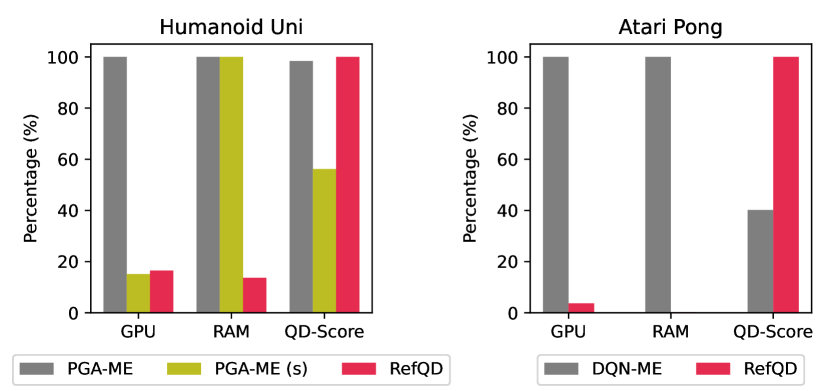
Figure 1: Performance and resource comparisons between RefQD and the baselines.

Our contributions are shown as follows.

• We are the first, to the best of our knowledge, to emphasize the importance of resource efficiency during the training phase of QD algorithms.

• We propose RefQD, a novel and effective method to enhance the resource efficiency of QD.

• Experimental results with limited resources demonstrate the effectiveness of RefQD, which utilizes only 3.7% to 16% GPU memories and achieves comparable or even superior QD metrics, including QD-Score, Coverage, and Max Fitness, with nearly the same wall-clock time and number of samples.

2 Background

2.1 Quality-Diversity

QD algorithms (Cully & Demiris, 2018; Chatzilygeroudis et al., 2021) aim to discover a diverse set of high-quality solutions for a given problem. Let $\mathcal{X}$ represent the solution space, and $\mathcal{S}\subseteq^{k}$ denote the $k$-dimensional behavior space of the solutions. The goal of QD algorithms is to maximize a fitness (quality) function $f:\mathcal{X}\to$ while exploring the $k$-dimensional behavior space $\mathcal{S}$ characterized by a given behavior descriptor function $\bm{m}:\mathcal{X}\to\mathcal{S}$. In the applications, the behavior space $\mathcal{S}$ can be given by an expert, trained with unsupervised learning methods (Grillotti & Cully, 2022), or learned from human feedback (Wang et al., 2023b; Ding et al., 2023).

Taking the widely recognized QD algorithm, MAP-Elites (ME) (Cully et al., 2015; Mouret & Clune, 2015), as an example, it maintains an archive by discretizing the behavior space $\mathcal{S}$ into $M$ cells $\{\mathcal{S}_{i}\}_{i=1}^{M}$ and storing at most one solution in each cell. The goal of ME is formalized as maximizing the sum $\sum\nolimits_{i=1}^{M}f({\bm{x}}_{i})$ of the fitness of the solutions in each cell, i.e., the QD-Score, where ${\bm{x}}_{i}$ denotes the solution contained within the cell $\mathcal{S}_{i}$, i.e., $\bm{m}({\bm{x}}_{i})\in\mathcal{S}_{i}$. If a cell $\mathcal{S}_{i}$ does not contain a solution, then the corresponding fitness value $f({\bm{x}}_{i})$ is considered as $0$. For simplicity, the fitness value $f(\cdot)$ is assumed (or transformed) to be non-negative to prevent the QD-Score from decreasing. The main process of ME consists of selecting parent solutions from the archive, generating offspring solutions through variation operators, evaluating the offspring solutions, and updating the archive (i.e., survivor selection). As the goal is to fill the cells with high-quality solutions, ME saves the solution with the best fitness in each cell in survivor selection.

Due to the inherent difficulty of obtaining a set of high-quality solutions with diverse behaviors, QD algorithms often require a large number of samples during optimization. Thus, how to improve the sample efficiency of QD has become a critical problem. Based on the improved components of QD (Cully & Demiris, 2018), recent studies can be roughly divided into two categories: how to select parent solutions from the archive (i.e., parent selection) (Lehman & Stanley, 2011; Cully & Demiris, 2018; Wang et al., 2022, 2023a), and how to update them to reproduce offspring solutions (i.e., variation) (Colas et al., 2020; Fontaine et al., 2020; Nilsson & Cully, 2021; Fontaine & Nikolaidis, 2021; Pierrot et al., 2022; Flageat et al., 2023). Apart from sample efficiency, the resource efficiency (e.g., GPU memory overhead during the training phase) is also a big issue of QD algorithms, which we will discuss in this work.

2.2 Archive Distillation

Some recent works have noticed the resources overhead of the QD algorithms in the deployment phase, and manage to reduce the resources of the final archive by archive distillation. Distilling the knowledge of an archive into a single policy is an alluring process that reduces the number of parameters output by the algorithm and enables generalization. Faldor et al. (2023) introduced the descriptor-conditioned gradient and distilled the experience of the archive into a single descriptor-conditioned actor. Macé et al. (2023) distilled the knowledge of the archive into a single decision transformer. Hegde et al. (2023) used diffusion models to distill the archive into a single generative model over policy parameters. These methods can achieve a high compression ratio while recovering most QD metrics. However, it is still required to maintain a large archive as well as a large number of solutions during the training process. Our proposed RefQD reduces the resource overhead in both the training and deployment phases. In addition, RefQD can also be combined with the archive distillation methods to obtain a single network. As an example, the deep decision archive of RefQD can be distilled to further reduce the resource overhead in the deployment phase.

3 Method

In this section, we will introduce the proposed RefQD method. RefQD follows the common procedure of QD algorithms, i.e., iterative parent selection, offspring solution reproduction, and archive updating. Inspired by the observation that the front and following layers of a neural network are used for state representation and decision-making, respectively (Zhou, 2021; Xue et al., 2024), RefQD decomposes a neural network into a representation part and a decision part (e.g., containing only the last layer of the neural network), and stores only decision parts in the archive while sharing a unique representation part, which will be introduced in Section 3.1. Such a strategy can improve the resource efficiency significantly, but also leads to the mismatch issue, i.e., a decision part in the archive fails to reproduce its behavior and fitness when combined with the latest shared representation part due to the frequent change of the representation part. Section 3.2 then introduces a series of strategies to overcome the mismatch issue, including periodic re-evaluation, maintaining a deep decision archive, top-$k$ re-evaluation, and learning rate decay for the representation part. In Section 3.3, we will present the RefQD method in detail along with its pseudo-codes in Algorithm 1.

3.1 Decomposition and Sharing

The low resource efficiency of QD algorithms is mainly due to the maintenance of too many solutions. However, in order to achieve sufficient diversity, it is unavoidable to maintain and update many solutions simultaneously. Therefore, to improve the resource efficiency, we try to reduce the total number of parameters of these solutions instead.

Considering the recent observation that different layers of a neural network have different functions (Chung et al., 2019; Dabney et al., 2021; Zhou, 2021; Hao et al., 2023; Xue et al., 2024), we divide a network into two parts, where the front layers with numerous parameters are considered as the representation part, and the few following layers are considered as the decision part. The knowledge learned by the representation part is usually common and can be shared, while the diverse behaviors can be generated by different decision parts. To significantly reduce the resource overhead, we maintain only one representation part, sharing it across all the decision parts in the archive and offspring population. In this way, we can reduce the RAM overhead from the archive and the GPU memory overhead from the offspring population simultaneously. This allows QD algorithms to be applied to larger scale problems with limited resources.

3.2 Overcoming Mismatch Issue

Mismatch issue. In the QD algorithms, it is expected for the solutions in each cell of the archive to reproduce the corresponding behaviors and fitness when they are selected as parent solutions or used in the deployment phase. Note that many decision parts in the archive can only reproduce the corresponding behaviors and fitness when combined with the corresponding versions of the representation parts at the time they were added to the archive. However, as we only maintain one representation part and do not save the representation parts of the solutions along with their decision parts in the archive, we can only use the latest version of the shared representation part to be combined with the decision parts. Since the latest representation part is being updated frequently during the iteration process, the decision parts in the archive may fail to reproduce their behaviors and fitness when combined with the latest shared representation part. Even worse, when a new decision part matching the latest version of the representation part attempts to add to the corresponding cell in the archive, it is likely to be eliminated by the decision part already in the cell with a better yet outdated performance record that it can no longer reproduce. We refer to this as the mismatch issue between the decision parts in the archive and the latest shared representation part.

Periodic re-evaluation. To address the mismatch issue, it is natural to periodically re-evaluate all the decision parts in the archive with the latest shared representation part, and add them back to the archive by survivor selection. However, we have observed that as the representation part changes frequently, there are a large number of “dead” decision parts in each time of re-evaluation, which have low fitness led by the mismatch issue and will be deleted in the survivor selection procedure. This will waste a lot of learned knowledge in the decision parts. In fact, many of the decision parts that do not match the current version of representation part can match a later one. Thus, only using periodic re-evaluation cannot address the mismatch issue.

Deep Decision Archive (DDA). To alleviate the wastage of learned knowledge led by periodic re-evaluation, RefQD weakens the elitist mechanism of QD by maintaining $K$ decision parts (e.g., $K=4$ in our experiments) instead of only one in each cell of the archive. That is, RefQD now maintains a DDA $\mathcal{A}=\{\mathcal{A}^{(i)}\}^{K}_{i=1}$ with $K$ levels, where each level of a cell in the archive stores one solution, and the fitness decreases as the level increases. Thus, the first level of DDA corresponds to the decision archive of traditional QD algorithms. Note that using a DDA brings a more robust exploration, because an inferior decision part when combined with the current representation part may become better when combined with later representation parts. When updating DDA, if the solution in the $i$-th level of a cell is replaced by survivor selection, it will not be removed directly, while the solution in the $K$-th level (i.e., the worst solution in the current cell) will be removed, and the solutions contained by the $i$-th to $(K-1)$-th level will move down one level accordingly. The idea of deep archive has also been used to solve uncentainty in noisy QD domains (Justesen et al., 2019; Flageat & Cully, 2020) and noisy general EAs (Qian et al., 2017; Qian, 2020). Note that the decision part is much smaller than the representation part. Thus, maintaining a DDA (i.e., storing multiple decision parts in each cell of the archive) will not significantly affect the resource efficiency.

Top-$k$ re-evaluation. Although using a DDA can reduce the wastage of learned knowledge, re-evaluating the entire DDA will need many samples and cost much time. To make a trade-off, we propose top-$k$ re-evaluation to re-evaluate only the solutions in the top $k$ levels of the DDA, as our final goal is to obtain a diverse set of high-quality solutions.

Learning rate decay for the representation part. The representation part changes frequently during the optimization of QD, making the decision parts hard to converge. Thus, we decay the learning rate of the representation part with iterations to improve the stability and allow the decision parts a better convergence.

Algorithm 1 Resource-efficient QD

Input: Number $T$ of total generations, number $N$ of selected solutions in each generation, number $M$ of cells of each level of DDA, period $T_{r}$ for re-evaluation, number $k$ of top levels of the archive to be re-evaluated
Output: Representation part ${\bm{x}^{\text{R}}}$, first level $\mathcal{A}^{(1)}$ of DDA

1:  Let $\mathcal{A}\leftarrow\emptyset$, $t\leftarrow 1$;

2:  while $t\leq T$ do

3:     if $t=1$ then

4:        ${\bm{x}^{\text{R}}},\{\bm{x}^{\text{D}}_{i}\}_{i=1}^{N}\leftarrow\texttt{Randomly\_Generate}(N)$

5:     else

6:        ${\bm{x}^{\text{R}}}\leftarrow\texttt{Train\_Representation}({\bm{x}^{\text{R}}},\mathcal{A})$;

7:        $\{\bm{x}^{\text{D}}_{i}\}_{i=1}^{N}\leftarrow\texttt{Parent\_Selection}(\mathcal{A},N)$;

8:        $\{{\bm{x}^{\text{D}}_{i}}^{\prime}\}_{i=1}^{N}\leftarrow\texttt{Variation}({\bm{x}^{\text{R}}},\{\bm{x}^{\text{D}}_{i}\}_{i=1}^{N})$

9:     end if

10:     $\texttt{Evaluation}({\bm{x}^{\text{R}}},\{{\bm{x}^{\text{D}}_{i}}^{\prime}\}_{i=1}^{N})$;

11:     $\mathcal{A}\leftarrow\texttt{DDA\_Selection}(\mathcal{A},\{{\bm{x}^{\text{D}}_{i}}^{\prime}\}_{i=1}^{N})$;

12:     $t\leftarrow t+1$;

13:     if $t\!\!\mod T_{r}=0$ then

14:        $\mathcal{A}^{\prime},\{\bm{x}^{\text{D}}_{i}\}_{i=1}^{M\times k}\leftarrow\texttt{Take\_Levels}(\mathcal{A},k)$;

15:        $\texttt{Re\_Evaluation}({\bm{x}^{\text{R}}},\{\bm{x}^{\text{D}}_{i}\}_{i=1}^{M\times k})$;

16:        $\mathcal{A}\leftarrow\texttt{DDA\_Selection}(\mathcal{A}^{\prime},\{\bm{x}^{\text{D}}_{i}\}_{i=1}^{M\times k})$

17:     end if

18:  end while

19:  return ${\bm{x}^{\text{R}}}$, $\mathcal{A}^{(1)}$

Algorithm 2 DDA Selection

Input: DDA $\mathcal{A}=\{\mathcal{A}^{(i)}\}^{K}_{i=1}$ with $K$ levels, decision parts $\{\bm{x}^{\text{D}}_{i}\}_{i=1}^{n}$ to be added
Output: Updated DDA $\mathcal{A}=\{\mathcal{A}^{(i)}\}^{K}_{i=1}$ with $K$ levels

1:  for $i=1$ to $n$ do

2:     $j\leftarrow\texttt{Get\_Cell\_Index}(\bm{m}(\bm{x}^{\text{D}}_{i}))$;

3:     $l\leftarrow 1$;

4:     while $l\leq K$ do

5:        if $\mathcal{A}^{(l)}_{j}=\emptyset$ then

6:           $\mathcal{A}^{(l)}_{j}\leftarrow\bm{\bm{x}^{\text{D}}}_{i}$;

7:           break

8:        else if $f(\mathcal{A}^{(l)}_{j})<f(\bm{x}^{\text{D}}_{i})$ then

9:           $\bm{z}\leftarrow\mathcal{A}^{(l)}_{j}$, $\mathcal{A}^{(l)}_{j}\leftarrow\bm{x}^{\text{D}}_{i}$, $\bm{x}^{\text{D}}_{i}\leftarrow\bm{z}$

10:        end if

11:        $l\leftarrow l+1$

12:     end while

13:  end for

14:  return $\mathcal{A}$

3.3 Resource-efficient QD

The procedure of RefQD is described in Algorithm 1. At the beginning, the DDA $\mathcal{A}$ is created as an empty set in line 1, and a shared representation part ${\bm{x}^{\text{R}}}$ and $N$ decision parts $\{\bm{x}^{\text{D}}_{i}\}_{i=1}^{N}$ are randomly generated in line 4. After that, in each generation $t$ (where $1<t\leq T$), RefQD first trains the representation part ${\bm{x}^{\text{R}}}$ in line 6, then selects $N$ decision parts $\{\bm{x}^{\text{D}}_{i}\}_{i=1}^{N}$ from the DDA $\mathcal{A}$ as parents in line 7, and finally combines each of them with the representation part ${\bm{x}^{\text{R}}}$ to form $N$ complete policies which are conducted by variation to generate $N$ offspring solutions $\{{\bm{x}^{\text{D}}_{i}}^{\prime}\}_{i=1}^{N}$ in line 8. After evaluating the generated offspring solutions $\{{\bm{x}^{\text{D}}_{i}}^{\prime}\}_{i=1}^{N}$ in line 10, we get the fitness and behavior of each solution. Then, we use these offspring solutions to update the DDA $\mathcal{A}$ in line 11, by employing Algorithm 2. After every $T_{r}$ iterations, top-$k$ re-evaluation is applied and the DDA $\mathcal{A}$ is updated accordingly, as shown in lines 14–16 of Algorithm 1. That is, the solutions $\{\bm{x}^{\text{D}}_{i}\}_{i=1}^{M\times k}$ in the top $k$ levels of the DDA $\mathcal{A}$ are re-evaluated by combining with the current representation part ${\bm{x}^{\text{R}}}$, and then used to update the DDA $\mathcal{A}^{\prime}$ which contains the remaining solutions after deleting $\{\bm{x}^{\text{D}}_{i}\}_{i=1}^{M\times k}$ from $\mathcal{A}$.

Algorithm 2 presents the procedure of using a set of decision parts (or called solutions) $\{\bm{x}^{\text{D}}_{i}\}_{i=1}^{n}$ to update a DDA $\mathcal{A}=\{\mathcal{A}^{(i)}\}^{K}_{i=1}$ with $K$ levels. Each solution $\bm{x}^{\text{D}}_{i}$ will be compared with the solutions archived in the corresponding cell (indexed by $j$ in line 2) of the DDA, from the top level to the bottom level (i.e., lines 4–12). If the current level $\mathcal{A}^{(l)}_{j}$ is empty, i.e., $\mathcal{A}^{(l)}_{j}=\emptyset$ in line 5, it will be occupied by $\bm{x}^{\text{D}}_{i}$ directly in line 6. If it is not empty and the contained solution is worse than $\bm{x}^{\text{D}}_{i}$ (i.e., $f(\mathcal{A}^{(l)}_{j})<f(\bm{x}^{\text{D}}_{i})$ in line 8), the current level $\mathcal{A}^{(l)}_{j}$ will also be occupied by $\bm{x}^{\text{D}}_{i}$, as $\mathcal{A}^{(l)}_{j}\leftarrow\bm{x}^{\text{D}}_{i}$ shown in line 9. In the latter case, the old solution in any level $\mathcal{A}^{(p)}_{j}$ (where $p\geq l$) will be moved to the following level $\mathcal{A}^{(p+1)}_{j}$, which is accomplished by using $\bm{x}^{\text{D}}_{i}$ to record the old solution in $\mathcal{A}^{(l)}_{j}$ (i.e., $\bm{z}\leftarrow\mathcal{A}^{(l)}_{j}$, $\bm{x}^{\text{D}}_{i}\leftarrow\bm{z}$ in line 9) and continuing the loop. Thus, if all the $K$ levels of cell $j$ have solutions, the solution in the last level $\mathcal{A}^{(K)}_{j}$, i.e., the worst solution, will be actually removed.

Note that the proposed RefQD is a general framework that can be implemented with different components. In our experiment, we will provide an implementation using the uniform parent selection and reproduction operators of PGA-ME (Nilsson & Cully, 2021; Flageat et al., 2023).

4 Experiment

4.1 Experimental Settings

To examine the performance of RefQD, we conduct experiments on the QDax suite and Atari environments.

QDax. It is a popular framework and benchmark for QD algorithms (Chalumeau et al., 2023b). We conduct experiments on five unidirectional tasks and three path-finding tasks. The unidirectional tasks aim to obtain a set of robot policies that run as fast as possible with different frequency of the usage of the feet, including Hopper Uni, Walker2D Uni, HalfCheetah Uni, Humanoid Uni, and Ant Uni. The reward is mainly determined by the forward speed of the robot, and the behavior descriptor is defined by the fraction of time each foot contacting with the ground. The path-finding tasks aim to obtain a set of robots that can reach each location on the given map, including Point Maze, Ant Maze, and Ant Trap. The behavior descriptor is defined as the final position of the robot. The reward is defined as the negative distance to the target position in Point Maze and Ant Maze, and the distance forward in Ant Trap. In all the tasks, the observation is a vector of sensor data, and the action is a vector representing the torque of each effector.

Atari. To further investigate the versatile of RefQD, we also conduct experiments on the video game Atari (Bellemare et al., 2013), which is a widely used benchmark in RL. The observation of Atari is an $84\times 84$ image of the video game, and the action is the discrete button to be pressed. We conduct experiments on two tasks, i.e., Pong and Boxing. For Pong, the one-dimensional behavior descriptor is defined as the frequency of the movement of the agent. For Boxing, the two-dimensional behavior descriptor is defined as the frequency of the movement and the frequency of the punches of the agent, respectively. The agent will receive positive and negative rewards when it wins or loses points in the games, respectively. Compared with QDax, Atari has a large image-based observation space and typically requires a larger CNN or ResNet (He et al., 2016) to process visual data, posing more challenges for the QD algorithms.

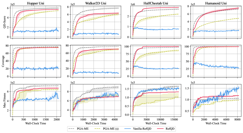
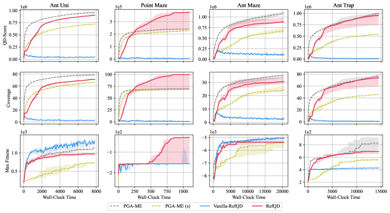
Figure 2: Performance comparison in terms of QD-Score, Coverage, and Max Fitness on eight environments of QDax. The medians and the first and third quartile intervals are depicted with curves and shaded areas, respectively.

To evaluate the effectiveness of RefQD, we compare the following methods.

• RefQD: Our proposed method.

• Vanilla-RefQD: The vanilla version of RefQD, which only uses decomposition and sharing, and does not use the strategies for overcoming the mismatch issue.

• PGA-ME or DQN-ME: PGA-ME / DQN-ME with the default settings. DQN-ME is the method that replaces TD3 (Fujimoto et al., 2018) with Double DQN (Mnih et al., 2015; Hasselt et al., 2016) in PGA-ME for the tasks with discrete action spaces on Atari.

• PGA-ME (s) or DQN-ME (s): PGA-ME / DQN-ME with a small number of offspring solutions, which have a much smaller GPU memory overhead compared to the default settings. However, they still maintain the whole archive (including many large representation parts), which costs lots of RAM, while all the RefQD variants do not need to.

We consider the following QD metrics: 1) QD-Score: The total sum of the fitness values across all solutions in the archive. It measures both the quality and the diversity of the solutions, which is the most important metric for the QD algorithms. 2) Coverage: The percentage of cells that have been covered by the solutions in the archive. It can measure the diversity of the solutions. 3) Max Fitness: The highest fitness value of the solutions in the archive. It can measure the quality of the solutions.

For a fair comparison, all the RefQD variants use the same reproduction operator with the compared method, i.e., same to PGA-ME on QDax and same to DQN-ME on Atari. All the RefQD variants use a decomposition strategy ($n+1$), i.e., use the last layer as the decision part and the rest as the representation part. In order to compare the performance under limited resources, all the methods are given the same amount of GPU memory, except for PGA-ME and DQN-ME, which are given unlimited GPU memory. In addition, it is not allowed to maintain the whole archive (i.e., to have cells that contain both representation and decision networks) for all methods, except for PGA-ME (DQN-ME) and PGA-ME (DQN-ME) (s), which have to store a full policy in each cell of the archive. Detailed settings can be found in Appendix A due to space limitation. Our code is available at https://github.com/lamda-bbo/RefQD.

4.2 Main Results

We plot the QD-Score, Coverage, and Max Fitness curves for different methods. Figure 2 and Table 1 show the results and the resource usage on eight environments of QDax, respectively. We can observe that RefQD with the limited resources, achieves the similar performance to PGA-ME that uses unlimited resources, and performs even better in HalfCheetah Uni, Humanoid Uni, and Point Maze. RefQD generally uses much less GPU memories, e.g., only using 16% GPU memories on Ant Uni compared to PGA-ME. PGA-ME (s) becomes extremely slow, performing significantly worse than RefQD and PGA-ME, although it still maintains the whole archive that costs lots of RAM. PGA-ME demonstrates the best overall QD-Score. However, it utilizes a substantial amount of GPU memories as well as a significant amount of RAM, as demonstrated in Figure 1. As is stated in Section 3.2, Vanilla-RefQD has the serious mismatch issue, resulting in the worst performance here.

Table 1: Resource usage and QD-Score comparisons of different methods on eight environments of QDax.

Tasks	PGA-ME			PGA-ME (s)			RefQD
	GPU	RAM	QD-Score	GPU	RAM	QD-Score	GPU	RAM	QD-Score
Hopper Uni	$100.0\%$	$100.0\%$	$100.0\%$	$13.3\%$	$100.0\%$	$76.5\%$	$14.2\%$	$4.5\%$	$92.7\%$
Walker2D Uni	$100.0\%$	$100.0\%$	$100.0\%$	$13.5\%$	$100.0\%$	$63.9\%$	$14.9\%$	$8.7\%$	$79.6\%$
HalfCheetah Uni	$100.0\%$	$100.0\%$	$100.0\%$	$13.5\%$	$100.0\%$	$74.0\%$	$14.9\%$	$8.6\%$	$104.6\%$
Humanoid Uni	$100.0\%$	$100.0\%$	$100.0\%$	$15.2\%$	$100.0\%$	$57.1\%$	$16.5\%$	$13.7\%$	$101.6\%$
Ant Uni	$100.0\%$	$100.0\%$	$100.0\%$	$14.3\%$	$100.0\%$	$67.8\%$	$16.0\%$	$9.2\%$	$84.4\%$
Point Maze	$100.0\%$	$100.0\%$	$100.0\%$	$13.3\%$	$100.0\%$	$88.7\%$	$14.0\%$	$3.2\%$	$85.0\%$
Ant Maze	$100.0\%$	$100.0\%$	$100.0\%$	$14.3\%$	$100.0\%$	$31.4\%$	$15.6\%$	$8.9\%$	$64.9\%$
Ant Trap	$100.0\%$	$100.0\%$	$100.0\%$	$14.3\%$	$100.0\%$	$57.4\%$	$15.6\%$	$9.0\%$	$107.1\%$

The experimental results and the resource usage on two Atari environments with CNN policy architecture are shown in Figure 3 and Table 2, respectively. Due to the complex observation space of Atari, DQN-ME and RefQD have a much larger representation part on this task, leading to a more obvious advantage of RefQD on the resource efficiency. Besides, the QD-Scores of RefQD on both tasks are also much better than those of DQN-ME. This is because the employed network decomposition can also simplify the optimization space of QD, thus making it easier to find better solutions, as also observed in CCQD (Xue et al., 2024).

We also conduct experiments on the Atari environments with ResNet policy architecture to examine the scalability of RefQD in challenging tasks with higher-dimensional decision space. The default settings of DQN-ME run out of memory and fail to work, while RefQD with limited resource performs significantly better than DQN-ME (s) with unlimited RAM, as shown in Table 3, demostrating that RefQD makes it possible to solve larger-scale QD problems efficiently. Due to space limitation, detailed results of QD metrics can be found in Appendix B.1.

Table 2: Resource usage and QD-Score comparisons of different methods using CNN as policy networks on two environments of Atari.

Tasks	DQN-ME			RefQD
	GPU	RAM	QD-Score	GPU	RAM	QD-Score
Pong	$100.0\%$	$100.0\%$	$100.0\%$	$3.7\%$	$0.3\%$	$248.6\%$
Boxing	$100.0\%$	$100.0\%$	$100.0\%$	$3.7\%$	$0.6\%$	$119.6\%$

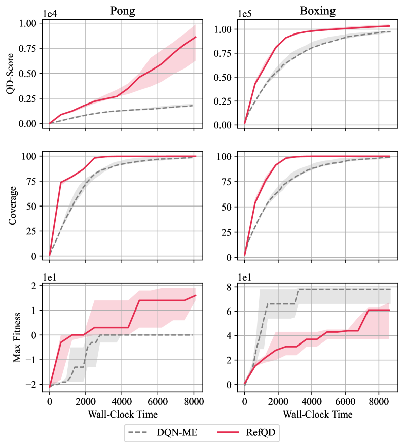
Figure 3: Performance comparison in terms of QD-Score, Coverage, and Max Fitness using CNN as policy networks on two environments of Atari. The medians and the first and third quartile intervals are depicted with curves and shaded areas, respectively.

Table 3: Resource usage and QD-Score comparisons of different methods using ResNet as policy networks on two environments of Atari.

Tasks	DQN-ME (s)			RefQD
	GPU	RAM	QD-Score	GPU	RAM	QD-Score
Pong	$100.0\%$	$100.0\%$	$100.0\%$	$52.5\%$	$2.5\%$	$220.1\%$
Boxing	$100.0\%$	$100.0\%$	$100.0\%$	$52.5\%$	$2.6\%$	$246.2\%$

4.3 Additional Results

We conduct additional experiments to deeply analyze the proposed RefQD, by investigating the influence of the decomposition strategy, the number $K$ of levels of DDA, the period $T_{r}$ of re-evaluations, and the number $k$ of top-$k$ re-evaluations. Other experiments, including ablation studies of RefQD, performance analysis based on time-steps, and experiments based on another state-of-the-art QD algorithm EDO-CS (Wang et al., 2022), are provided in Appendix B due to space limitation.

Influence of the decomposition strategy. Generally, the more we share, the less computational resources are required, but the greater potential for performance drop. We conduct experiments to analyze the influence of the decomposition strategies. When sharing less representation, RefQD has a better Max Fitness, due to the stronger ability from additional resource overhead, as shown in Appendix B.2. In practical use, the decomposition strategy can be set according to the available computational resources.

Influence of the number $K$ of levels of DDA. We analyze the influence of the number $K$ of levels of DDA, where $K$ is set to 1, 2, and 4 on all the eight tasks of QDax. The large $k$ DDA has, the more history knowledge will be saved in it, which also costs more RAM usage. As shown in Table 4, using $K=4$ achieves the best QD-Score on most tasks except for Ant Maze and Ant Trap. Larger $K$ may bring better QD-Score but also leads to the usage of more resources. Thus, we choose $4$ as the default value used in our experiments.

Table 4: QD-Score of RefQD by using different number $K$ of levels of DDA on eight environments of QDax.

Tasks	$K=1$	$K=2$	$K=4$
Hopper Uni	$472169$	$491220$	500594
Walker2D Uni	$423790$	$466840$	566845
HalfCheetah Uni	$2476923$	$2462211$	2629326
Humanoid Uni	$587483$	$632468$	646501
Ant Uni	$490440$	$678343$	715349
Point Maze	$188707$	$190907$	192868
Ant Maze	$620880$	738880	$669850$
Ant Trap	919987	$752117$	$741243$

Influence of the period $T_{r}$ of re-evaluations. Then, we perform the sensitivity analysis on the hyperparameter $T_{r}$. We compare three values of $T_{r}$, i.e., 20, 50, and 100. As shown in Figure 4, their performances on most environments are similar, but $T_{r}=50$ generally performs better. Thus, we use 50 as the default value for $T_{r}$.

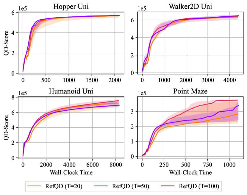
Figure 4: QD-Score of RefQD with different period $T_{r}$ of re-evaluation on four environments of QDax.

Influence of the number $k$ of top-$k$ re-evaluation. The top-$k$ re-evaluation strategy is proposed to make a trade-off between the number of re-evaluated samples and the consumed cost. Note that without the top-$k$ strategy, RefQD will use all the levels of DDA to re-evaluate. As shown in Figure 5, using a smaller $k$ will generally achieve a satisfactory performance, and we use $k=1$ in our experiments.

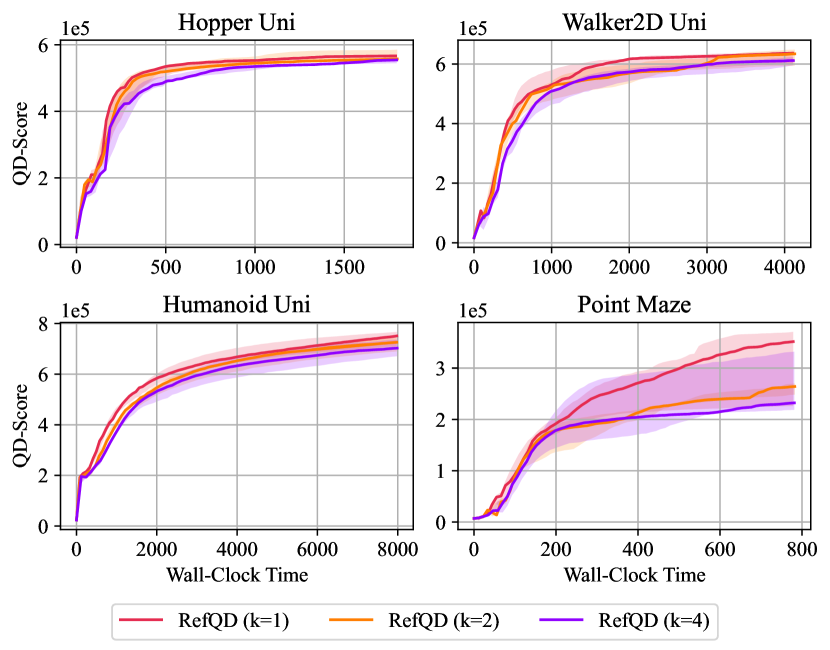
Figure 5: QD-Score of RefQD with different number $k$ of top-$k$ re-evaluation on four environments of QDax.

Ablation studies. We finally perform ablation studies on RefQD to analyze the effectiveness of each component, such as periodic re-evaluation, maintaining a DDA, top-$k$ re-evaluation, and learning rate decay for the representation part. The experimental results demonstrate their significance in enhancing the resource efficiency. Due to space limitation, detailed results can be found in Appendix B.3.

5 Conclusion

In this paper, we first emphasize the importance of resource efficiency during the training phase of QD algorithms and propose RefQD, a novel and effective method to enhance the resource efficiency of QD. Experimental results on the QDax suite and Atari environments with limited resources demonstrate the effectiveness of RefQD, which utilizes only 3.7% to 16% GPU memories of the well-known PGA-ME, and achieves comparable or even superior performance, with nearly the same wall-clock time and number of samples.

RefQD improves the resource efficiency of QD by considering the properties and principles of the QD algorithm itself, i.e., decomposing a neural network into a large representation part and a small decision part, and sharing the representation part with all decision parts. It is a general framework, which can be equipped with advanced sample-efficient operators to further improve the performance, and can also be combined with other general approaches such as model pruning to further decrease the computational overhead. The deep decision archive of RefQD can also be distilled into a single decision policy by archive distillation methods to reduce costs during the deployment phase. We hope this work can encourage the application of QD in more complex and challenging scenarios, such as embodied robots and large language models. One limitation of this paper is that we only examine the effectiveness of RefQD through empirical studies, without giving a mathematical theoretical analysis (Qian et al., 2024).

Impact Statement

This paper presents work whose goal is to advance the field of quality-diversity optimization. Our work enables more efficient use of computational resources in QD algorithms and applications, making it possible to solve large-scale quality-diversity optimization problems with limited resources.

Appendix A Detailed Settings

A.1 Algorithms

For a fair comparison, we unify the common hyperparameters of these methods on all the eight environments. The other hyperparameters of each method are set as the corresponding original paper.

The network structure on QDax is:

state $$\to\textbf{MLP}(256)\to\textbf{tanh}\to\textbf{MLP}(256)\to\textbf{tanh}\to\textbf{MLP}(\text{number of actions})\to\textbf{tanh}\to\text{action}$$

The CNN structure on Atari is:

state $$\to\textbf{CNN}(8\times 8\times 32)\to\textbf{leaky\_relu}\to\textbf{CNN}(4\times 4\times 64)\to\textbf{leaky\_relu}\to\textbf{CNN}(3\times 3\times 64)\to\textbf{leaky\_relu}$$

$$\to\textbf{MLP}(512)\to\textbf{leaky\_relu}\to\textbf{MLP}(\text{number of actions})\to\text{action}$$

The ResNet network structure on Atari is:

$$\text{state}\to\textbf{ResNet34}\to\textbf{MLP}(512)\to\textbf{leaky\_relu}\to\textbf{MLP}(\text{number of actions})\to\text{action}$$

Then, we introduce the two types of variation operators used in our experiments.

IsoLineDD. IsoLineDD (Vassiliades & Mouret, 2018) is a popular evolutionary operator used in several QD algorithms (Nilsson & Cully, 2021; Grillotti et al., 2023; Chalumeau et al., 2023a; Lim et al., 2023). Considering two parent solutions $\bm{x}_{1}$ and $\bm{x}_{2}$, the offspring solution $\bm{x}^{\prime}$ generated by the IsoLineDD operator is sampled as follows:

$$\bm{x}^{\prime}=\bm{x}_{1}+\sigma_{1}\cdot\mathcal{N}(\bm{0},\mathbf{I})+\sigma_{2}\cdot(\bm{x}_{2}-\bm{x}_{1})\cdot\mathcal{N}(0,1),$$

where $\sigma_{1}=0.005$ and $\sigma_{2}=0.05$ in this paper, $\mathbf{I}$ denotes the identity matrix, $\mathcal{N}(0,1)$ and $\mathcal{N}(\bm{0},\mathbf{I})$ denote a random number and a random vector sampled from the standard Gaussian distribution, respectively.

Policy gradient operators. The policy gradient operator maintains a critic and a greedy actor in many QD algorithms (Nilsson & Cully, 2021; Pierrot et al., 2022; Tjanaka et al., 2022; Chalumeau et al., 2023a; Lim et al., 2023), and we adopt this setting as well. At the start of each generation, the critic is trained with TD loss, while the greedy actor is simultaneously trained with policy gradient. Subsequently, the parent solutions are updated with policy gradient, using the critic in the variation process. We employ the policy gradient method TD3, whose hyperparameters are presented in Table 5.

Table 5: The hyperparameters of TD3.

Hyperparameter	Value
Critic hidden layer size	$[256,256]$
Policy learning rate	$1\times 10^{-3}$
Critic learning rate	$3\times 10^{-4}$
Replay buffer size	$1\times 10^{6}$
Training batch size	$32$
Policy training steps	$100$
Critic training steps	$300$
Reward scaling	$1.0$
Discount	$0.99$
Policy noise	$0.2$
Policy clip	$0.5$

Implementation of RefQD. We provide an implementation of RefQD using uniform parent selection and reproduction operators of PGA-ME in the experiment. The greedy actor of the reproduction operator is also decomposed into two parts, and the representation part of the greedy actor is also shared with other policies. To train the shared representation part, it is combined with the decision part of the greedy actor as well as several decision parts sampled from the decision archive to obtain the policy gradient. To train the decision part of the greedy actor and to variate the decision parts of the parent solutions, they are combined with the shared representation part to take actions.

Detailed settings of methods. The settings of the methods are summarized as follows.

• PGA-ME (Nilsson & Cully, 2021; Flageat et al., 2023) uses the IsoLineDD operator, and the policy gradient in the variation process. The proportion of the offspring solutions generated by the two operators is both $0.5$, which is the same as (Nilsson & Cully, 2021; Lim et al., 2023).

• PGA-ME (s) is the same as PGA-ME, except that the population size is set to $8$ to make it have a similar GPU memories usage to RefQD.

• DQN-ME uses the DQN as the policy to handle the discrete action space in Atari.

• RefQD uses the variation operator as same as PGA-ME. The number of levels of the DDA is $4$, and the top level is re-evaluated every $50$ iterations.

A.2 Computational Resources

All the experiments are conducted on an NVIDIA RTX 3090 GPU (24 GB) with an AMD Ryzen 9 3950X CPU (16 Cores).

Appendix B Additional Results

B.1 More Complex Policy Architectures

To examine the scalability of RefQD in challenging tasks with higher-dimensional decision space, we also conduct experiments in the Atari environments with ResNet policy architecture. Due to the high-dimensional decision spaces, the default settings of DQN-ME run out of memory and fail to work. Thus, we compare our method with DQN-ME (s), which has a small number of offspring solutions, using smaller GPU memory than the default settings but still requiring to maintain the whole archive in unlimited RAM. As shown in Figure 6, RefQD with limited resources achieves significantly better performance than DQN-ME (s).

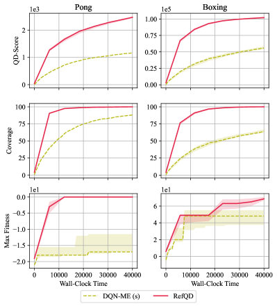
Figure 6: Performance comparison in terms of QD-Score, Coverage, and Max Fitness using ResNet as policy networks on two environments of Atari. The medians and the first and third quartile intervals are depicted with curves and shaded areas, respectively.

B.2 Decomposition Strategies

The decomposition strategy is a crucial setting as it significantly impacts resource utilization. For example, when computational resources are very limited, the representation part should be shared as much as possible to reduce overhead, just as we do in the default settings in our paper. Generally, the more we share, the less computational resources are required, but the greater potential for performance drop. We conduct experiments to analyze the influence of the decomposition strategies. We compare the performance of (2+1) and (1+2), where (2+1) denotes that the representation part and decision part have 2 and 1 layers, respectively, and (1+2) denotes that they have have 1 and 2 layers, respectively. As shown in Figure 7, when sharing less representation, RefQD has a better Max Fitness, due to the stronger ability from additional resource overhead. In practical use, the decomposition strategy of RefQD can be set according to the available computational resources. It can also be adaptive based on the task or network architecture.

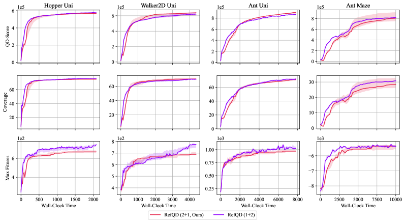
Figure 7: Performance comparison with different decomposition strategies in terms of QD-Score, Coverage, and Max Fitness. The medians and the first and third quartile intervals are depicted with curves and shaded areas, respectively.

B.3 Ablation Studies

We also consider the following variants of RefQD:

• RefQD w/o TR: The same as RefQD, except that it does not use top-$k$ re-evaluation (TR), but re-evaluates the whole archive.

• RefQD w/o TR & LRD: The same as RefQD w/o TR, except that it does not use the learning rate decay (LRD) of the representation part.

• Vanilla-RefQD w/ Re-SS (i.e., RefQD w/o TR, LRD, & DDA): The same as Vanilla-RefQD, except that it performs the re-survivor selection (Re-SS).

As shown in Figure 8, Vanilla-RefQD has the serious mismatch issue and does not perform well. Vanilla-RefQD w/ Re-SS performs even worse, as it may waste a lot of learned knowledge in the decision parts. RefQD performs the best, and removing the top-$k$ re-evaluation or the learning rate decay for the representation part results in a performance degradation.

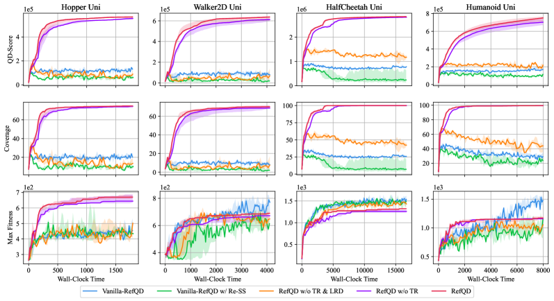
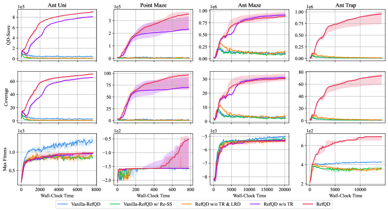
Figure 8: Performance comparison in terms of QD-Score, Coverage, and Max Fitness in ablation studies. The medians and the first and third quartile intervals are depicted with curves and shaded areas, respectively.

B.4 Time-steps vs. QD metrics

Apart from the wall-clock time, we also compare the sample efficiency of the methods. As shown in Figure 9, RefQD with limited resources also achieves similar sample efficiency to PGA-ME and PGA-ME (s), and performs even better in HalfCheetah Uni, Humanoid Uni, and Point Maze.

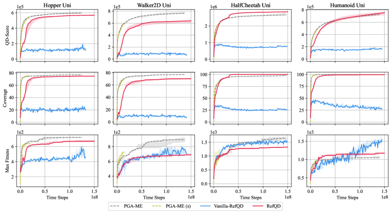
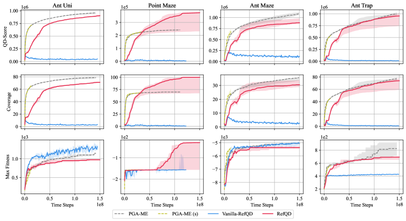
Figure 9: Performance comparison in terms of QD-Score, Coverage, and Max Fitness w.r.t. the number of time-steps. The medians and the first and third quartile intervals are depicted with curves and shaded areas, respectively.

B.5 Combined with EDO-CS

RefQD is a general method that can be integrated with different QD algorithms. We also adopt EDO-CS (Wang et al., 2022) as another QD algorithm. As shown in Figure 10, the EDO-CS variant of RefQD with limited resources also achieves similar or better performance than the original version of EDO-CS, demostrating the generalization of RefQD.

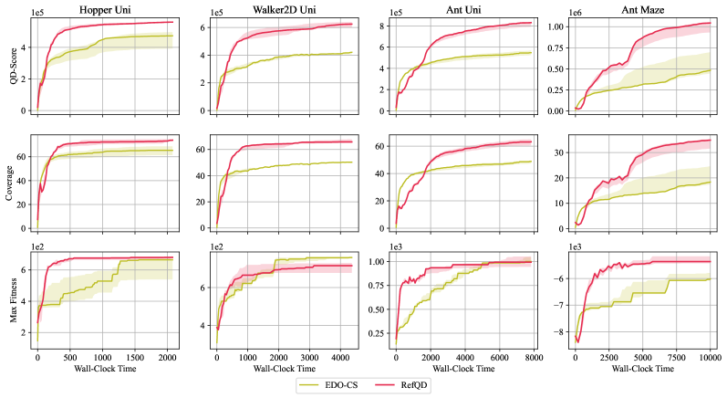
Figure 10: Performance comparison of EDO-CS-based methods in terms of QD-Score, Coverage, and Max Fitness. The medians and the first and third quartile intervals are depicted with curves and shaded areas, respectively.

References

- Bäck (1996) Bäck, T. Evolutionary Algorithms in Theory and Practice: Evolution Strategies, Evolutionary Programming, Genetic Algorithms. Oxford University Press, 1996.
- Bellemare et al. (2013) Bellemare, M. G., Naddaf, Y., Veness, J., and Bowling, M. The arcade learning environment: An evaluation platform for general agents. Journal of Artificial Intelligence Research, 47:253–279, 2013.
- Bhatt et al. (2022) Bhatt, V., Tjanaka, B., Fontaine, M. C., and Nikolaidis, S. Deep surrogate assisted generation of environments. In Advances in Neural Information Processing Systems 35 (NeurIPS), New Orleans, LA, 2022.
- Chalumeau et al. (2023a) Chalumeau, F., Boige, R., Lim, B., Macé, V., Allard, M., Flajolet, A., Cully, A., and Pierrot, T. Neuroevolution is a competitive alternative to reinforcement learning for skill discovery. In The 11th International Conference on Learning Representations (ICLR), Kigali, Rwanda, 2023a.
- Chalumeau et al. (2023b) Chalumeau, F., Lim, B., Boige, R., Allard, M., Grillotti, L., Flageat, M., Macé, V., Flajolet, A., Pierrot, T., and Cully, A. QDax: A library for quality-diversity and population-based algorithms with hardware acceleration. arXiv:2308.03665, 2023b.
- Chatzilygeroudis et al. (2021) Chatzilygeroudis, K., Cully, A., Vassiliades, V., and Mouret, J.-B. Quality-diversity optimization: A novel branch of stochastic optimization. In Black Box Optimization, Machine Learning, and No-Free Lunch Theorems, pp. 109–135. Springer, 2021.
- Chung et al. (2019) Chung, W., Nath, S., Joseph, A., and White, M. Two-timescale networks for nonlinear value function approximation. In The 7th International Conference on Learning Representations (ICLR), New Orleans, LA, 2019.
- Colas et al. (2020) Colas, C., Madhavan, V., Huizinga, J., and Clune, J. Scaling MAP-Elites to deep neuroevolution. In Proceedings of the 22nd ACM Genetic and Evolutionary Computation Conference (GECCO), pp. 67–75, Cancún, Mexico, 2020.
- Cully & Demiris (2018) Cully, A. and Demiris, Y. Quality and diversity optimization: A unifying modular framework. IEEE Transactions on Evolutionary Computation, 22(2):245–259, 2018.
- Cully et al. (2015) Cully, A., Clune, J., Tarapore, D., and Mouret, J.-B. Robots that can adapt like animals. Nature, 521(7553):503–507, 2015.
- Dabney et al. (2021) Dabney, W., Barreto, A., Rowland, M., Dadashi, R., Quan, J., Bellemare, M. G., and Silver, D. The value-improvement path: Towards better representations for reinforcement learning. In Proceedings of the 35th AAAI Conference on Artificial Intelligence (AAAI), pp. 7160–7168, Virtual, 2021.
- Ding et al. (2023) Ding, L., Zhang, J., Clune, J., Spector, L., and Lehman, J. Quality diversity through human feedback. arXiv:2310.12103, 2023.
- Ecoffet et al. (2021) Ecoffet, A., Huizinga, J., Lehman, J., Stanley, K. O., and Clune, J. First return, then explore. Nature, 590(7847):580–586, 2021.
- Eysenbach et al. (2018) Eysenbach, B., Gupta, A., Ibarz, J., and Levine, S. Diversity is all you need: Learning skills without a reward function. In The 6th International Conference on Learning Representations (ICLR), Vancouver, Canada, 2018.
- Faldor et al. (2023) Faldor, M., Chalumeau, F., Flageat, M., and Cully, A. MAP-Elites with descriptor-conditioned gradients and archive distillation into a single policy. arXiv:2303.03832, 2023.
- Flageat & Cully (2020) Flageat, M. and Cully, A. Fast and stable map-elites in noisy domains using deep grids. In Proceedings of the 32nd IEEE Symposium on Artificial Life (ALife), pp. 273–282, Virtual, 2020.
- Flageat et al. (2023) Flageat, M., Chalumeau, F., and Cully, A. Empirical analysis of PGA-MAP-Elites for neuroevolution in uncertain domains. ACM Transactions on Evolutionary Learning and Optimization, 3(1):1–32, 2023.
- Fontaine & Nikolaidis (2021) Fontaine, M. C. and Nikolaidis, S. Differentiable quality diversity. In Advances in Neural Information Processing Systems 34 (NeurIPS), pp. 10040–10052, Virtual, 2021.
- Fontaine et al. (2020) Fontaine, M. C., Togelius, J., Nikolaidis, S., and Hoover, A. K. Covariance matrix adaptation for the rapid illumination of behavior space. In Proceedings of the 22nd ACM Genetic and Evolutionary Computation Conference (GECCO), pp. 94–102, Cancún, Mexico, 2020.
- Fontaine et al. (2021) Fontaine, M. C., Liu, R., Khalifa, A., Modi, J., Togelius, J., Hoover, A. K., and Nikolaidis, S. Illuminating mario scenes in the latent space of a generative adversarial network. In Proceedings of the 35th AAAI Conference on Artificial Intelligence (AAAI), pp. 5922–5930, Virtual, 2021.
- Fujimoto et al. (2018) Fujimoto, S., van Hoof, H., and Meger, D. Addressing function approximation error in actor-critic methods. In Proceedings of the 35th International Conference on Machine Learning (ICML), pp. 1582–1591, Stockholm, Sweden, 2018.
- Grillotti & Cully (2022) Grillotti, L. and Cully, A. Unsupervised behavior discovery with quality-diversity optimization. IEEE Transactions on Evolutionary Computation, 26(6):1539–1552, 2022.
- Grillotti et al. (2023) Grillotti, L., Flageat, M., Lim, B., and Cully, A. Don’t bet on luck alone: Enhancing behavioral reproducibility of quality-diversity solutions in uncertain domains. arXiv:2304.03672, 2023.
- Hao et al. (2023) Hao, J., Li, P., Tang, H., Zheng, Y., Fu, X., and Meng, Z. ERL-Re2: Efficient evolutionary reinforcement learning with shared state representation and individual policy representation. In The 11th International Conference on Learning Representations (ICLR), Kigali, Rwanda, 2023.
- Hasselt et al. (2016) Hasselt, H. v., Guez, A., and Silver, D. Deep reinforcement learning with double Q-learning. In Proceedings of the 30th AAAI Conference on Artificial Intelligence (AAAI), pp. 2094–2100, Phoenix, Arizona, 2016.
- He et al. (2016) He, K., Zhang, X., Ren, S., and Sun, J. Deep residual learning for image recognition. In Proceedings of the 29th IEEE Conference on Computer Vision and Pattern Recognition (CVPR), pp. 770–778, Las Vegas, NV, 2016.
- Hegde et al. (2023) Hegde, S., Batra, S., Zentner, K. R., and Sukhatme, G. S. Generating behaviorally diverse policies with latent diffusion models. arxiv:2305.18738, 2023.
- Justesen et al. (2019) Justesen, N., Risi, S., and Mouret, J.-B. Map-elites for noisy domains by adaptive sampling. In Proceedings of the 21st Genetic and Evolutionary Computation Conference (GECCO), pp. 121–122, Lille, France, 2019.
- Kumar et al. (2020) Kumar, S., Kumar, A., Levine, S., and Finn, C. One solution is not all you need: Few-shot extrapolation via structured MaxEnt RL. In Advances in Neural Information Processing Systems 34 (NeurIPS), pp. 8198–8210, Virtual, 2020.
- Lehman & Stanley (2011) Lehman, J. and Stanley, K. O. Evolving a diversity of virtual creatures through novelty search and local competition. In Proceedings of the 13th ACM Genetic and Evolutionary Computation Conference (GECCO), pp. 211–218, Dublin, Ireland, 2011.
- Lim et al. (2023) Lim, B., Allard, M., Grillotti, L., and Cully, A. Accelerated quality-diversity through massive parallelism. Transactions on Machine Learning Research, 2023.
- Lupu et al. (2021) Lupu, A., Hu, H., and Foerster, J. Trajectory diversity for zero-shot coordination. In Proceedings of the 38th International Conference on Machine Learning (ICML), pp. 7204–7213, Virtual, 2021.
- Macé et al. (2023) Macé, V., Boige, R., Chalumeau, F., Pierrot, T., Richard, G., and Perrin-Gilbert, N. The quality-diversity transformer: Generating behavior-conditioned trajectories with decision transformers. In Proceedings of the Genetic and Evolutionary Computation Conference (GECCO), pp. 1221–1229, Lisbon, Portugal, 2023.
- Miao et al. (2022) Miao, J., Zhou, T., Shao, K., Zhou, M., Zhang, W., Hao, J., Yu, Y., and Wang, J. Promoting quality and diversity in population-based reinforcement learning via hierarchical trajectory space exploration. In Proceedings of the 39th IEEE International Conference on Robotics and Automation (ICRA), pp. 7544–7550, Philadelphia, PA, 2022.
- Mnih et al. (2015) Mnih, V., Kavukcuoglu, K., Silver, D., Rusu, A. A., Veness, J., Bellemare, M. G., Graves, A., Riedmiller, M. A., Fidjeland, A. K., Ostrovski, G., Petersen, S., Beattie, C., Sadik, A., Antonoglou, I., King, H., Kumaran, D., Wierstra, D., Legg, S., and Hassabis, D. Human-level control through deep reinforcement learning. Nature, 518(7540):529–533, 2015.
- Mouret & Clune (2015) Mouret, J.-B. and Clune, J. Illuminating search spaces by mapping elites. arXiv:1504.04909, 2015.
- Nilsson & Cully (2021) Nilsson, O. and Cully, A. Policy gradient assisted MAP-Elites. In Proceedings of the 23rd ACM Genetic and Evolutionary Computation Conference (GECCO), pp. 866–875, Lille, France, 2021.
- Pierrot et al. (2022) Pierrot, T., Macé, V., Chalumeau, F., Flajolet, A., Cideron, G., Beguir, K., Cully, A., Sigaud, O., and Perrin-Gilbert, N. Diversity policy gradient for sample efficient quality-diversity optimization. In Proceedings of the 24th ACM Genetic and Evolutionary Computation Conference (GECCO), pp. 1075–1083, Boston, MA, 2022.
- Qian (2020) Qian, C. Distributed pareto optimization for large-scale noisy subset selection. IEEE Transactions on Evolutionary Computation, 24(4):694–707, 2020.
- Qian et al. (2017) Qian, C., Shi, J.-C., Yu, Y., Tang, K., and Zhou, Z.-H. Subset selection under noise. In Advances in Neural Information Processing Systems 30 (NIPS), pp. 3563–3573, Long Beach, CA, 2017.
- Qian et al. (2024) Qian, C., Xue, K., and Wang, R. Quality-diversity algorithms can provably be helpful for optimization. In Proceedings of the 31st International Joint Conference on Artificial Intelligence (IJCAI), 2024.
- Salehi et al. (2022) Salehi, A., Coninx, A., and Doncieux, S. Few-shot quality-diversity optimization. IEEE Robotics and Automation Letters, 7(2):4424–4431, 2022.
- Samvelyan et al. (2024) Samvelyan, M., Raparthy, S. C., Lupu, A., Hambro, E., Markosyan, A. H., Bhatt, M., Mao, Y., Jiang, M., Parker-Holder, J., Foerster, J., Rocktaschel, T., and Raileanu, R. Rainbow teaming: Open-ended generation of diverse adversarial prompts. arXiv:2402.16822, 2024.
- Sfikas et al. (2021) Sfikas, K., Liapis, A., and Yannakakis, G. N. Monte carlo elites: quality-diversity selection as a multi-armed bandit problem. In Proceedings of the 23rd Genetic and Evolutionary Computation Conference (GECCO), pp. 180–188, Lille, France, 2021.
- Shah & Kumar (2021) Shah, R. M. and Kumar, V. RRL: Resnet as representation for reinforcement learning. In Proceedings of the 38th International Conference on Machine Learning (ICML), pp. 9465–9476, Virtual, 2021.
- Strouse et al. (2021) Strouse, D., McKee, K., Botvinick, M., Hughes, E., and Everett, R. Collaborating with humans without human data. In Advances in Neural Information Processing Systems 34 (NeurIPS), pp. 14502–14515, Virtual, 2021.
- Tjanaka et al. (2022) Tjanaka, B., Fontaine, M. C., Togelius, J., and Nikolaidis, S. Approximating gradients for differentiable quality diversity in reinforcement learning. In Proceedings of the 24th ACM Genetic and Evolutionary Computation Conference (GECCO), pp. 1102–1111, Boston, MA, 2022.
- Tylkin et al. (2021) Tylkin, P., Radanovic, G., and Parkes, D. C. Learning robust helpful behaviors in two-player cooperative atari environments. In Dignum, F., Lomuscio, A., Endriss, U., and Nowé, A. (eds.), Proceedings of the20th International Conference on Autonomous Agents and Multiagent Systems (AAMAS), Virtual, pp. 1686–1688, Virtual, 2021.
- Vassiliades & Mouret (2018) Vassiliades, V. and Mouret, J.-B. Discovering the elite hypervolume by leveraging interspecies correlation. In Proceedings of the 20th Genetic and Evolutionary Computation Conference (GECCO), pp. 149–156, Kyoto, Japan, 2018.
- Wang et al. (2023a) Wang, R., Xue, K., Shang, H., Qian, C., Fu, H., and Fu, Q. Multi-objective optimization-based selection for quality-diversity by non-surrounded-dominated sorting. In Proceedings of the 32nd International Joint Conference on Artificial Intelligence (IJCAI), pp. 4335–4343, Macao, SAR, China, 2023a.
- Wang et al. (2023b) Wang, R., Xue, K., Wang, Y., Yang, P., Fu, H., Fu, Q., and Qian, C. Diversity from human feedback. arXiv:2310.06648, 2023b.
- Wang et al. (2022) Wang, Y., Xue, K., and Qian, C. Evolutionary diversity optimization with clustering-based selection for reinforcement learning. In Proceedings of the 10th International Conference on Learning Representations (ICLR), Virtual, 2022.
- Xue et al. (2024) Xue, K., Wang, R., Li, P., Li, D., Hao, J., and Qian, C. Sample-efficient quality-diversity by cooperative coevolution. In Proceedings of the 12th International Conference on Learning Representations (ICLR), Vienna, Austria, 2024.
- Zhang et al. (2023) Zhang, Y., Fontaine, M. C., Bhatt, V., Nikolaidis, S., and Li, J. Multi-robot coordination and layout design for automated warehousing. In Proceedings of the 32nd International Joint Conference on Artificial Intelligence (IJCAI), pp. 5503–5511, Macao, SAR, China, 2023.
- Zhou (2021) Zhou, Z.-H. Why over-parameterization of deep neural networks does not overfit? Science China Information Sciences, 64:1–3, 2021.
- Zhou (2023) Zhou, Z.-H. A theoretical perspective of machine learning with computational resource concerns. arXiv:2305.02217, 2023.
- Zhou et al. (2019) Zhou, Z.-H., Yu, Y., and Qian, C. Evolutionary Learning: Advances in Theories and Algorithms. Springer, 2019.