FastGAS: Fast Graph-based Annotation Selection for In-Context Learning

Abstract

In-context learning (ICL) empowers large language models (LLMs) to tackle new tasks by using a series of training instances as prompts. Since generating the prompts needs to sample from a vast pool of instances and annotate them (e.g., add labels in classification task), existing methods have proposed to select a subset of unlabeled examples for annotation, thus enhancing the quality of prompts and concurrently mitigating annotation costs. However, these methods often require a long time to select instances due to their complexity, hindering their practical viability. To address this limitation, we propose a graph-based selection method, FastGAS, designed to efficiently identify high-quality instances while minimizing computational overhead. Initially, we construct a data similarity graph based on instance similarities. Subsequently, employing a graph partitioning algorithm, we partition the graph into pieces. Within each piece (i.e., subgraph), we adopt a greedy approach to pick the most representative nodes. By aggregating nodes from diverse pieces and annotating the corresponding instances, we identify a set of diverse and representative instances for ICL. Compared to prior approaches, our method not only exhibits superior performance on different tasks but also significantly reduces selection time. In addition, we demonstrate the efficacy of our approach in LLMs of larger sizes.

1 Introduction

Recent advances in natural language processing heavily leverage large language models, exemplified by models such as GPT-3 Brown et al. (2020). Among them, in-context learning (ICL) emerges as a promising direction in this field. ICL adapts specific tasks with just a few instances as prompts, offering a viable alternative to traditional supervised fine-tuning Liu et al. (2023). The performance of ICL is intricately tied to the effectiveness of the prompt surface, encompassing factors such as instance selection and the sequence of demonstration instances Zhao et al. (2021); Dong et al. (2022); Lu et al. (2021); Wang et al. (2023b). In this study, we focus on instance selection and explore novel solutions to reduce manual annotation costs while maintaining high in-context learning performance.

Previous research underscores the importance of retrieving prompts from a vast set of annotated instances to achieve optimal performance Liu et al. (2021); Rubin et al. (2021). In particular, performance is shown to improve significantly when choosing in-context examples similar to each test input Liu et al. (2021). However, addressing the unique requirements of different test instances requires a large set of annotated examples, incurring significant human and financial resources.

To mitigate annotation costs, previous efforts have sought to identify a small number of unlabeled instances for annotation Su et al. (2022a); Zhang et al. (2023). The objective is to select diverse and representative instances, where representativeness aids in finding similar demonstrations for different test instances, while diversity broadens the overall coverage. Despite their superiority over random selection, these methods have specific drawbacks. For example, Vote-$k$ Su et al. (2022a) emphasizes diversity but adds inference costs due to predictions on unlabeled data. IDEAL Zhang et al. (2023) employs influence-driven selective annotations, drawing inspiration from influence maximization in social graphs. However, both methods struggle to balance diversity and representativeness, leading to suboptimal performance.

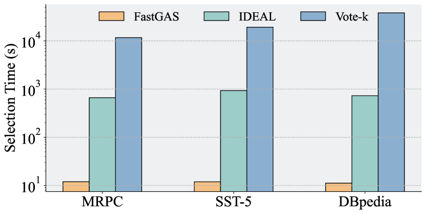
Figure 1: Comparison of our method and two baselines on three classification tasks (MPRC, SST-5, and DBpedia) with respect to time consumption during subset selection. The annotation budget is $18$. The y-axis represents the time consumption with a log scale. Notably, our method significantly reduces the time cost in comparison to both baseline methods.

Furthermore, a notable shortcoming of existing methods is their computational inefficiency. The precise calculation process (e.g., iteratively searching the entire dataset) results in high computational costs, making them less practical for real-world applications. Figure 1 illustrates the time required by our method and two baseline methods, Vote-$k$ and IDEAL, under the same hardware conditions and annotation budgets. It is observed that both baselines necessitate at least $500$ seconds to select a subset for DBpedia and SST-5 tasks. Remarkably, for the DBpedia task, Vote-$k$ exceeds $30,000$ seconds (over eight hours) to select just 18 instances. As the annotation budget grows, the time needed by these methods to perform the selection process can increase exponentially (See Section 4.4), further constraining their applicability in real-world settings. In our pursuit of an efficient and effective selective annotation method, we pose the fundamental question: Can we identify a set of diverse and representative instances with high efficiency?

Answering this question, we propose FastGAS, a Fast Graph-based Annotation Selection method that works in an unsupervised manner. We first build a data similarity graph based on the similarity among unlabeled data. We then select instances for annotation based on the data similarity graph. In particular, our method focuses on the following three properties of selected instances:

• Diversity: We perform graph partitioning to separate the data similarity graph into segments. We treat each segment as a set of instances. We ensure the diversity of selected instances by selecting them from different segments.

• Representiveness: For each segment, we select instances with the max corresponding node degree in the data similarity graph. The selected instances thus can maximally cover the subgraph and guarantee their representativeness.

• Efficiency: We apply a multi-level graph bisection algorithm to speed up the graph partitioning process. For the selection of each segment, we apply a simple but effective greedy algorithm. Compared to baseline methods that iteratively select over the entire graph, applying the greedy algorithm on each component can reduce the computation time.

Compared with state-of-the-art baseline methods, our method improves the overall performance on seven datasets in three types of tasks. Besides, for all tasks, our method only needs a few seconds to complete the instance selection process. In addition, we also provide a theoretical guarantee for the effectiveness of the greedy selection algorithm.

2 Related Work

In-Context Learning    In-context learning (ICL) integrates a small number of training examples as prompts before the test input Brown et al. (2020), demonstrating a remarkable ability to enhance the performance of large language models (LLMs) in a wide range of downstream tasks, such as machine translation Agrawal et al. (2022); Sia and Duh (2023), data generation Ye et al. (2022), and others Wang et al. (2021b); He et al. (2023); Panda et al. (2023). Furthermore, the advent of advanced strategies such as chain-of-thought prompting Wei et al. (2022) has significantly refined the efficacy of ICL, offering deeper insights and more nuanced understanding within this innovative paradigm Kim et al. (2022); Chan et al. (2022); Srivastava et al. (2022); Bansal et al. (2022).

Despite its successes, ICL’s efficacy is often hampered by the sensitivity to the choice of in-context examples, leading to research on optimized selection strategies Liu et al. (2021); Lu et al. (2021); Zhao et al. (2021); Shi et al. (2024). Techniques have evolved from selecting examples close to the test input in embedding spaces Liu et al. (2021); Wu et al. (2022); Gao et al. (2020); Rubin et al. (2021). The focus has also shifted towards annotation efficiency, exploring how to find a set of examples once for all queries on the same task Zhang et al. (2023); Su et al. (2022a); Chang and Jia (2023). Following existing works Zhang et al. (2023); Su et al. (2022a), we also use a graph to represent unlabeled instances and employ graph-based methods to select instances for annotation. However, our methodology distinguishes itself from existing works by focusing on efficiency in the selection of instances. As discussed in Section 1, we aim to select diverse and representative instances while reducing the computation cost.

Active Learning    Given a limited budget for labeling, active learning empowers machine learning models to achieve comparable or superior performance using a carefully selected set of labeled training instances Cohn et al. (1994); Settles (2009); Wang et al. (2023a). Our work on selective annotation aligns with the goal of active learning applied to graphs, specifically focusing on the selection of nodes for labeling to inform predictions Cai et al. (2017); Jia et al. (2019); Wang et al. (2021a, 2022). Traditional graph-based active learning methods employ criteria such as uncertainty Settles and Craven (2008) and representativeness  Li and Guo (2013) for selection. Since the ICL tasks we focus on do not involve model training or finetuning, we compare our method with basic graph active learning methods that are not incorporated with model training, like those based on node degree Cai et al. (2017); Wang et al. (2021a) and PageRank Rodriguez (2008). Our experiments indicate that while simple graph active learning methods work well in ICL, our approach still achieves better overall performance.

3 Methods

In this section, we will explain how to integrate a graph partition algorithm and a greedy algorithm in a selective annotation in in-context learning to reduce the annotation cost.

3.1 Problem Setup

We first give the definition of the selective annotation problem. In-context learning is a paradigm that allows language models to learn tasks given only a few examples in the form of demonstration Brown et al. (2020). Specifically, LLMs perform in-context learning tasks based on a task-specific prompt $\mathcal{Z}$ formed by concatenating $M$ labeled training examples $\mathcal{Z}=[\mathbf{z}_{1},...,\mathbf{z}_{M}]$, where each $\mathbf{z}_{i}$ represents one labeled example $(\mathbf{x}_{i},\mathbf{y}_{i})$ consisting of the instance $\mathbf{x}_{i}$ and label $\mathbf{y}_{i}$ (e.g., the answer of a question based on the instance). In the real world, we usually only have unlabeled samples $\mathcal{X}=\{\mathbf{x}_{i}\}_{i=1}^{N}$, and obtaining large-scale annotated examples for ICL requires substantial manpower and financial resources.

Selective annotation aims at selecting a subset $\mathcal{L}\subset\mathcal{X}$ to be annotated, where $|\mathcal{L}|=M$ is the annotation budget, such that ICL only using prompts retrieved from the selected subset can yield good performance on the test set and thus reduce the annotation cost.

3.2 Fast Graph-based Annotation Selection

For the selective annotation problem, it is essential to find a subset that covers vast unlabeled data. To achieve this, we design a graph-based annotation method that balances the diversity and representativeness of the annotated samples. Briefly, we build a data similarity graph by assessing the similarity of unlabeled data embeddings. We partition the data similarity graph into distinct subgraphs by employing a multi-level graph bisection algorithm, and each subgraph is treated as a candidate set. Through a stepwise, greedy selection process of the most influential data nodes in each subgraph, we generate subsets that encapsulate the subgraph’s information. Ultimately, we aggregate these subsets from all subgraphs to represent the unlabeled data. We will now provide a detailed, step-by-step explanation of the aforementioned process.

Data Similarity Graph Generation.    By averaging the resulting vectors over the text input words, we compute the vector representation for each unlabeled training instance using Sentence-BERT Reimers and Gurevych (2019). We then use the embedding vectors to create the data similarity graph $\mathcal{G}=(\mathcal{V},\mathcal{E})$ where each vertex $v_{i}\in\mathcal{V}$ represents an unlabeled instance $x_{i}\in\mathcal{X}$ as defined above. For each vertex $v\in\mathcal{V}$, we introduce edges connecting it to its $k$ nearest neighbors in terms of cosine similarity and get $\mathcal{E}$.

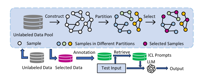
Figure 2: An overview FastGAS. Given the unlabeled data pool, we initially construct a graph based on data similarity. This graph is then partitioned into distinct components. Within each component, we employ a greedy algorithm to select nodes until we reach the annotation budget. The selected instances are annotated and subsequently used to retrieve ICL prompts for the task.

Graph Partitioning.    We aim to enhance instance diversity by strategically selecting instances from various regions within the data similarity graph. The division of regions process can be conceptualized as addressing a $K$-way graph partitioning problem, where the goal is to effectively divide the graph into $K$ distinct components with approximately equal numbers of vertices but with few edges crossing between components. The formal definition of the graph partitioning problem is defined as follows: given a graph $\mathcal{G}=(\mathcal{V},\mathcal{E})$ with $|\mathcal{V}|=N$, partition $\mathcal{V}$ into $K$ subsets, $\mathcal{V}_{1},\mathcal{V}_{2},...,\mathcal{V}_{K}$ such that $\mathcal{V}_{i}\cap\mathcal{V}_{j}=\emptyset$ for $i\neq j$, $|\mathcal{V}_{i}|$ is close $N/K$, $\bigcup_{i}\mathcal{V}_{i}=\mathcal{V}$, and the number of edges of $\mathcal{E}$ whose incident vertices belong to different subsets is minimized.

The $K$-way graph partitioning problem is an NP-complete problem. We tend to use recursive bisection to find an approximate solution with an acceptable execution time. Specifically, we first obtain a 2-way partition of $\mathcal{G}$, and then we recursively bisect the two segments independently. After log$K$ phases, $\mathcal{G}$ is partitioned into $K$ different components. Unfortunately, graph bisection is also NP-complete and has several inherent shortcomings Hendrickson et al. (1995). In order to improve efficiency, we apply a multi-level graph bisection algorithm to produce high-quality partitions at low cost Karypis and Kumar (1998). It consists of the following three phases:

• Coarsening phase: The graph $\mathcal{G}$ is transformed into a sequence of smaller graphs $\mathcal{G}_{1},\mathcal{G}_{2},...,\mathcal{G}_{m}$ such that $|\mathcal{V}|>|\mathcal{V}_{1}|>|\mathcal{V}_{2}|>\cdots>|\mathcal{V}_{m}|$.

• Partitioning phase: A 2-way partition $P_{m}$ of the graph $\mathcal{G}_{m}=(\mathcal{V}_{m},\mathcal{E}_{m})$ is computed that partitions $\mathcal{V}_{m}$ into two subgraphs, each containing half the vertices of $\mathcal{G}$.

• Uncoarsening phase: The partition $P_{m}$ of $\mathcal{G}_{m}$ is projected back to $\mathcal{G}$ by going through intermediate partitions $P_{m-1},P_{m-2},...,P_{1},P_{0}$.

For more detailed methods of each phase, we will include them in Appendix C.

Greedy Node Selection.    The graph partitioning operation divides the data similarity graph into $K$ disjoint components, ensuring diversity by treating each component as a set of instances. However, further discussion is required on the selection of suitable instances that exhibit significant representativeness for each subgraph. Following the graph partitioning process, which yields $K$ subgraphs with a similar number of nodes denoted as $|\mathcal{V}_{i}|=N/K$, and considering an annotation budget $|\mathcal{L}|=M$, our objective is to choose $n=M/K$ instances within each subgraph. To mitigate potential challenges associated with high memory and computation costs, we employ a greedy selection method. In detail, for the subgraph $\mathcal{G}_{i}$, we first select the node $v_{i}^{1}$ that has the largest degree: $v_{i}^{1}=\operatorname*{argmax}_{v\in\mathcal{G}_{j}}d(v)$. Then, we update the subgraph $\mathcal{G}_{i}$ by removing the selected node $v_{i}^{1}$ and the edges connecting $v_{i}^{1}$: $\mathcal{G}_{i}=\mathcal{G}_{i}\setminus v_{i}^{1}$. The above steps are repeated $n$ times to get the selected node set $\mathcal{V}_{i}^{sel}=\{v_{i}^{1},...,v_{i}^{n}\}$, and the corresponding instances $\mathcal{X}_{i}^{sel}=\{x_{i}^{1},...,x_{i}^{n}\}$ are chosen to represent the instances belonging to the subgraph $\mathcal{G}_{i}$. The iterative form can be written as

$$v_{i}^{j}=\operatorname*{argmax}_{v\in\mathcal{G}_{i}\setminus\{v_{i}^{k}|k\in[1,j-1]\}}d(v)$$ (1)

Specifically, the greedy selection algorithm guarantees the following property, demonstrating its ability to enhance the representativeness of the selected instances.

Proposition 3.1.

Given the budget $n$ and graph $\mathcal{G}$, the greedy algorithm will select $\mathcal{V}^{sel}=\{v^{1},...,v^{n}\}$ that maximize the number of edges within $\mathcal{V}^{sel}$ and those connecting $\mathcal{V}^{sel}$ and $\mathcal{G}\setminus\mathcal{V}^{sel}$.

$$\mathcal{V}^{sel} =\operatorname*{argmax}_{|\mathcal{V}|=n}|\{(u,v)|u,v\in\mathcal{V}\}|$$

$$+|\{(u,v)|u\in\mathcal{V}\hskip 3.61371pt{\rm and}\hskip 3.61371ptv\in\mathcal{G}\setminus\mathcal{V}\}|$$

Remark 1.

The greedy selection process on subgraphs can be conceptualized as a divide-and-conquer approach to selection on the entire graph, leading to improved algorithmic efficiency. Specifically, when the annotation budget $M$ is considerably smaller than the total number of nodes $N$ (i.e., $M\ll N$), the computational cost of greedy selection on the entire graph is $\mathcal{O}(2MN)$, while the cost incurred on the $K$ subgraphs is significantly reduced to $\mathcal{O}\big{(}{\frac{2MN}{K}}\big{)}$.

Prompt Retrieval.    Upon obtaining a set of instances $\mathcal{L}=\bigcup_{i}\mathcal{X}_{i}^{sel}$ through the greedy selective annotation process, we manually annotate $\mathcal{L}$ to create a comprehensive set of labeled instances. Consistent with previous studies, we leverage Sentence-BERT Reimers and Gurevych (2019) to generate embeddings for all annotated instances and identify the most similar instances to each test input based on cosine similarity.

4 Experiment

In this section, we evaluate the effectiveness of our method in various datasets encompassing diverse task categories. We begin by presenting the details of our experiment setups. Subsequently, the reported results demonstrate the superior performance of the proposed method in identifying an optimal selective annotation subset efficiently, outperforming established baselines. Furthermore, we conduct ablation studies to investigate the impact of crucial hyperparameters in our method.

4.1 Setups

Datasets and Models    We conduct extensive experiments in seven diverse datasets, which include six distinct tasks detailed in Table 4. Following existing works, each dataset adheres to the standard train/dev/test split provided by the Transformers library Wolf et al. (2019). For datasets with publicly available test data (SST-5, XSUM, and DBpedia), we utilize the test set for evaluation. In cases where test data is not publicly accessible, consistent with previous works Zhang et al. (2023); Su et al. (2022a), we employ the dev data for evaluation. Evaluation metrics include precision for all classification and multiple-choice selection datasets and ROUGE-L Lin (2004) for XSUM.

Unless explicitly mentioned, we conduct all experiments using the GPT-J-6B model Wang and Komatsuzaki (2021). Additionally, we present results from tests on other models such as GPT-Neo-2.7B Black et al. (2021), OPT-6.7B Zhang et al. (2022), as well as more advanced models including Llama-2-7B-Chat Touvron et al. (2023) and GPT-3.5-Turbo OpenAI (2023).

Baselines    In our main experiments, we conduct a comprehensive evaluation of FastGAS against random selection and two state-of-the-art selective annotation baselines: Vote-$k$ Su et al. (2022a) and IDEAL Zhang et al. (2023). Additionally, we benchmark FastGAS against other widely recognized methods in selecting core sets from extensive unlabeled data pools. These methods include (1) Top-degree Wu et al. (2019), which selects nodes with the largest degrees until the annotation budget is met; (2) PageRank Cai et al. (2017), which is used to score node representativeness in graph-based active learning; (3) Subclustering Chen et al. (2023), which initially clusters instances into $K$ groups via $K$-means, then further subdivides each into $M/K$ subclusters for centroid instance selection; and (4) Louvain Blondel et al. (2008), which utilizes the Louvain community detection algorithm for graph partitioning and a greedy selection algorithm akin to FastGAS for instance selection from each community.

To emulate real-world conditions, we follow Vote-$k$ Su et al. (2022a) and IDEAL Zhang et al. (2023), selectively annotating from a pool of 3,000 instances randomly subsampled from the original training data for each task. For robustness, we conduct this subsampling procedure three times per experiment, and the reported results represent the average across three trials.

Hyperparameter Setting    In our main experiment, we create a data similarity graph for all unlabeled instances by linking each vertex to its ten nearest neighbors $(k=10)$. For the baseline methods, we follow their hyperparameter settings to construct directed graphs Zhang et al. (2023); Su et al. (2022a). Regarding the selection of $K$ for graph partitioning, we adjust $K$ within $\{2,3,6,9\}$ for an annotation budget of $18$, and within $\{2,5,10,25,50\}$ for a budget of $100$, identifying an optimal $K$ for each task. Our method’s selection time is significantly shorter than that of the baselines (Section 4.4), making the time spent finding the appropriate $K$ negligible. We align our annotation budgets of $18$ and $100$ with those used in Vote-$k$ Su et al. (2022a) and IDEAL Zhang et al. (2023), choosing $18$ specifically because it allows all annotated examples to fit within the context limits of LLMs without necessitating prompt retrieval. The impacts of $k$ and $K$ are detailed in Sections 4.3 and 4.5, respectively.

4.2 Main Result

Table 1 presents a comparison between FastGAS and other baseline methods across annotation budgets of $|\mathcal{L}|\in\{18,100\}$. FastGAS outperforms the two existing baselines in nearly all scenarios ($13$ out of $14$). Notably, with an annotation budget of $18$, all annotated examples fit within the prompt limitations of LLMs, making the evaluation results a direct reflection of the quality of selected instances Zhang et al. (2023). When the annotation budget is $18$, FastGAS performs better than the baseline on most datasets, which shows that FastGAS can select higher-quality data. While the proposed active learning baselines outshine in specific instances (e.g., the Subclustering method excels in the DBpedia task for both annotation budgets), their general performance is hindered by their approach to balancing representativeness and diversity of the selected instances. For example, methods like Top-degree and PageRank prioritize representativeness Cai et al. (2017). Overall, FastGAS generally surpasses these baselines ($10$ out of $14$), demonstrating its effectiveness. Furthermore, as a deterministic selective annotation method, FastGAS operates based on a given set of unlabeled samples, mirroring the advantage seen with Vote-$k$. This means that the variability in FastGAS’s performance stems exclusively from the manner in which unlabeled samples are gathered. This significantly enhances the robustness of ICL by ensuring consistency in the selection process Su et al. (2022a). We provide detailed results that contain the maximum and minimum values of each task in Appendix F.

Table 1: The results of FastGAS and six baselines on seven distinct datasets with annotation budgets of $100$ and $18$, utilizing similarity-based prompt retrieval for all methods. We report the average results with three different runs for each method. Bold fonts indicate the best performance, while underlines denote the second-best results.

$|\mathcal{L}|$	Methods	Classification					Multi-Choice	Generation
		MRPC	SST-5	MNLI	DBpedia	RTE	HellaSwag	XSUM
100	Random	64.32	49.61	38.15	89.84	55.34	64.71	17.24
100	Vote-$k$	64.60	46.61	38.93	89.19	57.68	65.89	19.55
100	IDEAL	65.49	49.87	41.02	90.63	58.98	64.97	19.68
100	Top-degree	62.76	42.32	41.02	83.85	51.69	66.67	19.39
100	PageRank	64.84	40.71	44.17	83.72	53.38	66.01	19.55
100	Subclustering	64.84	49.48	41.28	92.32	57.55	65.62	19.18
100	Louvain	59.63	39.58	41.14	86.33	53.52	65.89	19.27
100	FastGAS	66.15	50.26	42.06	90.76	61.98	67.45	20.00
18	Random	55.47	42.97	37.76	83.20	54.95	65.49	16.63
18	Vote-$k$	56.90	41.78	39.45	88.02	56.64	66.02	19.45
18	IDEAL	63.80	44.92	39.58	83.20	53.65	65.89	19.21
18	Top-degree	48.57	39.45	41.93	77.34	54.43	65.76	20.05
18	PageRank	46.09	39.71	40.49	79.04	56.07	65.89	19.82
18	Subclustering	61.46	46.05	37.63	89.06	56.63	65.76	19.49
18	Louvain	61.33	38.02	38.02	83.59	55.86	65.62	20.23
18	FastGAS	65.23	46.61	44.53	88.93	56.51	66.67	20.26

4.3 Effect of $k$

We compare FastGAS and other graph-based baselines with respect to different $k$ for the construction of the graph, and the result is shown in Figure 3. Initially, our method consistently exceeds other graph-based baselines in various settings. Second, we observe that the ideal $k$ value varies among different methods and datasets. Specifically, for the MNLI dataset, most methods perform better with $k=10$. We also conclude that, for FedGAS, $k$ must be carefully balanced, neither too large nor too small. A smaller $k$ value, as well as a larger one, impedes the ability to differentiate between distinct representative nodes in the graph, complicating the selection process by potentially choosing multiple similar nodes. Concurrently, a larger $k$ value could also increase the computational time.

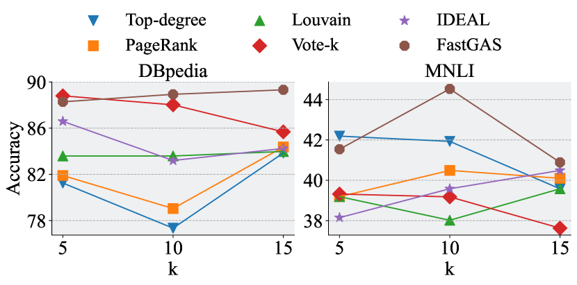
Figure 3: Comparison of our method and other graph-based baselines with respect to different $k$ for the construction of the graph.

4.4 Evaluating Time Efficiency

In Section 1, we illustrate that FastGAS drastically reduces the time cost compared to two existing methods with an annotation budget of $18$. Figure 4 expands on this by showing the time consumption of our method and two baselines for an annotation budget of $100$. Relative to Figure 1, the time needed for FastGAS does not increase much. This is because the most time-intensive processes in FastGAS, i.e., constructing and partitioning the data similarity graph, are not affected by the annotation budget. In contrast, the time costs of the two baselines, especially IDEAL, increase sharply; for nearly all tasks, IDEAL and Vote-$k$ require more than eight hours for selection. As the annotation budget increases, the efficiency of FastGAS in example selection becomes even more pronounced.

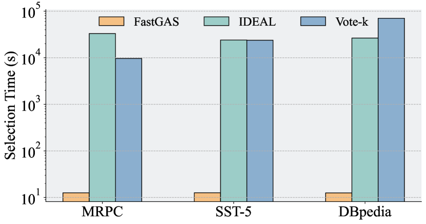
Figure 4: Comparison of our method and two baselines on three classification tasks (MPRC, SST-5, and DBpedia) with respect to time consumption during subset selection. The annotation budget is $100$. The y-axis represents the time consumption with a log scale.

4.5 Effect of Number of Partitions

The hyperparameter $K$ plays a critical role in graph partitioning, determining the number of components into which the graph is divided. We explore $K$’s impact on FastGAS and offer insights for adjusting it. Figure 5 illustrates FastGAS’s performance in three datasets with an annotation budget of $100$. The figure demonstrates that enhancing $K$ up to a certain point improves FastGAS’s performance; however, the increase beyond this optimal threshold does not result in further performance gains. A small $K$ results in relatively rough partitioning, such that significantly different data points are grouped into the same subgraph. Selecting through coarsely partitioned subgraphs can obscure meaningful distinctions in the data, resulting in the loss of the diversity of the selected nodes. Conversely, with a sufficiently large $K$, the graph partitioning algorithm results in more edges being cut during the partitioning process, thus affecting the degree of nodes in each disjoint subgraph. As a result, nodes with a large degree in the original graph may lose a large number of edges due to partitioning and thus be ignored by the greedy algorithm. This alteration hampers the greedy algorithm’s ability to select representative nodes effectively. Hence, a balanced $K$ value facilitates the optimal performance of FastGAS by ensuring a balance of representativeness and diversity.

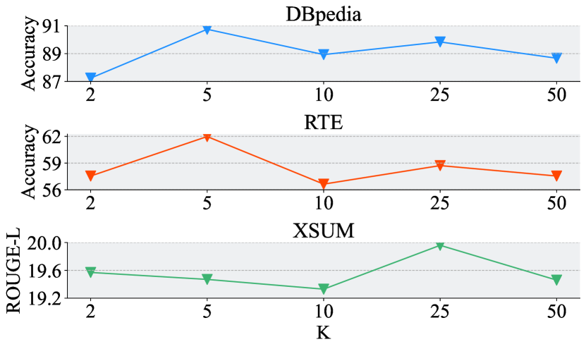
Figure 5: Performance of FastGAS across different numbers of partitions with an annotation budget of $100$.

4.6 Random Prompt Retrieval

In Section 4.2, we evaluate the performance of FastGAS against other baselines using a similarity-based prompt retrieval method. Building on previous research Zhang et al. (2023); Su et al. (2022a), we investigate the impact of employing a random retrieval method, specifically, by randomly selecting labeled instances as prompts for each test instance under the annotation budget $100$ and $18$. The findings are presented in Table 2. We note a marked decline in the effectiveness of selective annotation methods under large annotation budgets when prompts are chosen through random selection. This deterioration may stem from the increased likelihood of selecting instances from the larger labeled pool that are less relevant to the test sample, as determined by their distance in the embedding space Liu et al. (2021). Significantly, FastGAS continues to outperform the two baseline methods across all datasets, even when employing random retrieval. With an annotation budget of $18$, all annotated instances fit within the prompt capacity of LLMs, making the order of instances the only difference between the two prompt retrieval methods. The performance of FastGAS underscores its capability to produce a more reliable training subset for ICL tasks Chang and Jia (2023).

Table 2: Comparison of random and similar prompt retrieval. The selection approach, when paired with a similarity-based prompt retrieval method, generally outperforms its counterpart, which utilizes a random prompt retrieval technique.

Methods			Datasets
$|\mathcal{L}|$	Selection	Retrieval	MRPC	MNLI	HellaSwag
100	Vote-$k$	Similar	64.60	38.93	65.89
100	IDEAL	Similar	65.49	41.02	64.97
100	FastGAS	Similar	66.15	42.06	67.45
100	Vote-$k$	Random	60.67	37.76	64.58
100	IDEAL	Random	62.50	39.06	66.80
100	FastGAS	Random	62.50	40.88	67.32
18	Vote-$k$	Similar	56.90	39.45	66.02
18	IDEAL	Similar	63.80	39.58	65.89
18	FastGAS	Similar	65.23	44.53	66.67
18	Vote-$k$	Random	54.56	41.02	66.54
18	IDEAL	Random	64.19	38.15	66.54
18	FastGAS	Random	64.71	44.01	67.19

4.7 Evaluation on Different Language Models

We conduct evaluations of FastGAS on various language models, including GPT-Neo 2.7B Black et al. (2021), OPT-6.7B Zhang et al. (2022), Llama-2-7B-Chat Touvron et al. (2023), and GPT-3.5-Turbo OpenAI (2023), applying the same instructions across each dataset. Table 3 shows the performance of three selective annotation methods on smaller language models (GPT-Neo 2.7B and OPT-6.7B) across three datasets, where FastGAS overall surpasses two baseline annotation methods. Notably, OPT-6.7B exhibits lower performance on the XSUM summarization task compared to other LLMs, a finding echoed in Tam et al. (2022). However, FastGAS remains superior to the baselines even when using the OPT-6.7B model.

Table 3: Comparative performance of FastGAS versus baselines using GPT-Neo-2.7B and OPT-6.7B models across various datasets with an annotation budget of $18$. FastGAS generally outperforms baseline methods across a variety of models and datasets.

Methods		Datasets
Selection	Model	MRPC	DBpedia	XSUM
Vote-$k$	GPT-Neo-2.7B	57.42	80.73	19.45
IDEAL	GPT-Neo-2.7B	65.89	78.38	19.69
FastGAS	GPT-Neo-2.7B	66.02	80.86	20.15
Vote-$k$	OPT-6.7B	36.59	88.02	6.86
IDEAL	OPT-6.7B	45.18	83.20	6.13
FastGAS	OPT-6.7B	44.66	88.93	6.89

Further experiments on more advanced LLMs are presented in Figure 6, confirming FastGAS’s enhanced performance with larger language models. This underscores FastGAS as a versatile approach effective across LLMs of varying sizes. Particularly, the performance leap with GPT-3.5-Turbo, especially notable on the MNLI dataset (improving from 50.18% with Llama-2-7B-Chat to 70.18% with GPT-3.5-Turbo), highlights the advantage of larger models equipped with more parameters and extensive training data, thereby bolstering their capability in classification tasks.

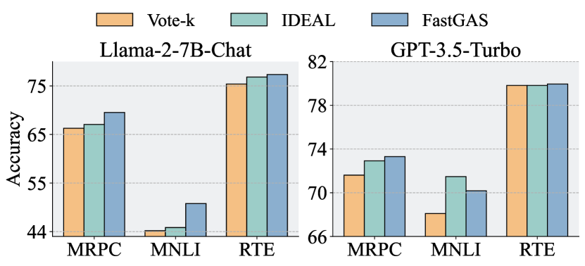
Figure 6: Comparative performance of FastGAS versus baselines using Llama-2-7B-Chat and GPT-3.5-Turbo models across various datasets with an annotation budget of $18$.

5 Conclusion

Recent advancements have showcased the capability of large language models (LLMs) to adapt to new tasks with just a few demonstration instances. While existing approaches aim to enhance model performance by selecting a limited number of instances to annotate for prompts, they are hindered by significant computational demands and lengthy processing times. To address these challenges, we introduce a graph-based selection algorithm, FastGAS, accompanied by a theoretical analysis of its effectiveness. Our empirical evaluations reveal that this method outperforms others in seven distinct tasks, demonstrating exceptional efficacy. Unlike conventional methods that require high computation costs, our method greatly improves the efficiency of selecting instances, substantially enhancing its applicability to practical scenarios. Additionally, we demonstrate FastGAS’s versatility across LLMs of various sizes. We hope that these insights will help researchers in devising effective ICL strategies to optimize LLM performance.

6 Limitation

The primary constraint of our study is the inability to automatically select the most appropriate number of partitions ($K$) and the most appropriate number of neighbors ($k$) during the data similarity graph construction. Given the relatively short execution time of our method, conducting multiple trials to identify the ideal $K$ and $k$ value is viable. However, the cost of the inference phase could restrict the feasibility of such extensive experimentation in practical settings. To enhance efficiency, FastGAS adopts a greedy selection process that is carried out separately for each piece. However, we have not explored how the interrelations between samples across different graph pieces influence the overall instance selection. Additionally, due to hardware limitations and available time, our research only covered LLMs up to 7B in size. Future investigations will aim to assess FastGAS’s efficacy with larger LLMs and across a broader array of tasks.

7 Ethics Statement

This work introduces FastGAS, a graph-based selective annotation method that can effectively and efficiently select high-quality instances for in-context learning tasks. While acknowledging the need for responsible usage of the proposed method, we do not foresee major negative societal impacts.

8 Acknowledgements

This work was supported in part by the US National Science Foundation (NSF) under awards ECCS-2332060, CPS-2313110, ECCS-2143559, ECCS-2033671, SII-2132700, IIS-2006844, IIS-2144209, IIS-2223769, CNS2154962, and BCS-2228534, and the Commonwealth Cyber Initiative under awards VV-1Q23-007, HV-2Q23-003, and VV-1Q24-011.

Appendix A General experimental conditions

Our implementation of FastGAS and baselines is primarily conducted using PyTorch Paszke et al. (2019). For the GPT-3.5-Turbo experiments, we utilize the OpenAI API. The models GPT-J-6B, GPT-Neo 2.7B, Llama-2-7B-Chat, and OPT-6.7B are sourced from the Huggingface Transformers Library Wolf et al. (2019). All experiments are performed on a single NVIDIA RTX A6000 GPU with 48GB of memory.

Appendix B The Detailed Information of Seven Datasets

Table 4: The detailed information of seven datasets

	Dataset	Task
Classification	MRPC Dolan et al. (2004)	Paraphrase Detection
	SST-5 Socher et al. (2013)	Sentiment Analysis
	DBpedia Lehmann et al. (2015)	Topic Classification
	MNLI Williams et al. (2018)	Natural Language Inference
	RTE Bentivogli et al. (2009)	Natural Language Inference
Multiple-Choice	HellaSwag Zellers et al. (2019)	Commonsense Reasoning
Generation	XSUM Narayan et al. (2018)	Summarization

Appendix C Detailed Graph Partition Algorithm

• Coarsening phase: The graph $\mathcal{G}$ is transformed into a sequence of smaller graphs $\mathcal{G}_{1},\mathcal{G}_{2},...,\mathcal{G}_{m}$ such that $|\mathcal{V}|>|\mathcal{V}_{1}|>|\mathcal{V}_{2}|>\cdots>|\mathcal{V}_{m}|$.

• Partitioning phase: A 2-way partition $P_{m}$ of the graph $\mathcal{G}_{m}=(\mathcal{V}_{m},\mathcal{E}_{m})$ is computed that partitions $\mathcal{V}_{m}$ into two parts, each containing half the vertices of $\mathcal{G}$.

• Uncoarsening phase: The partition $P_{m}$ of $\mathcal{G}_{m}$ is projected back to $\mathcal{G}$ by going through intermediate partitions $P_{m-1},P_{m-2},...,P_{1},P_{0}$

Coarsening phase    Due to the construction of the data similarity graph, the degree of most vertices is close to the graph’s average degree. To generate coarser graphs, we employ a strategy of finding a random matching and merging the matched vertices into a multi-node Bui and Jones (1993); Hendrickson et al. (1995). A graph’s matching is a set of edges, each pair of which shares no common vertex. We create a subsequent coarser graph, $\mathcal{G}_{i+1}$, from $\mathcal{G}_{i}$ by matching in $\mathcal{G}_{i}$ and merging the matched vertices. We utilize a random algorithm akin to those detailed in Bui and Jones (1993); Hendrickson et al. (1995).

The algorithm operates as follows: vertices are processed in a random sequence. For an unmatched vertex $u$, an unmatched adjacent vertex $v$ is randomly chosen, and the edge $(u,v)$ is added to the matching. If there is no unmatched adjacent vertex for $u$, then $u$ remains unmatched in this random matching process. The computational complexity of this algorithm is $\mathcal{O}(|\mathcal{E}|)$.

Partitioning phase    To efficiently bisect the graph, we simply initiate from a vertex and expand a region around it using a breadth-first approach until half of the vertices are encompassed Ciarlet Jr and Lamour (1996); Goehring and Saad (1994). Given that the bisection quality is highly dependent on the initial vertex selection Karypis and Kumar (1998), we employ a strategy similar to Karypis and Kumar (1998), wherein we randomly select 10 vertices and subsequently expand 10 distinct regions from each. The trail yielding the smallest edge cut is then chosen for the partition.

Uncoarsening phase    During the uncoarsening phase, as each vertex $u\in\mathcal{G}_{i+1}$ represents a unique subset $\mathcal{U}$ of vertices from $\mathcal{G}_{i}$, we derive partition $P_{i}$ from $P_{i+1}$ by assigning the vertices in $\mathcal{U}$ to the same part that vertex $u$ belongs to. Although $P_{i+1}$ may represent a local minimum partition for $\mathcal{G}_{i+1}$, the corresponding partition $P_{i}$ might not be at a local minimum with respect to $\mathcal{G}_{i}$. To refine this uncoarsened partition, we employ the KL algorithm Kernighan and Lin (1970), which iteratively searches for and swaps subsets of vertices between partitions to achieve a lower edge cut. This swapping process continues until no further improvements can be made, indicating that the partition has reached a local minimum.

Appendix D Proof of Proposition 3.1

Proof.

We employ an inductive approach to demonstrate that the node set $\mathcal{V}^{sel}$, selected by the greedy algorithm, satisfies the maximum cover property,

$$\mathcal{V}^{sel}=\operatorname*{argmax}_{|\mathcal{V}|=n}|\{(u,v)|u,v\in\mathcal{V}\}|+|\{(u,v)|u\in\mathcal{V}\hskip 3.61371pt{\rm and}\hskip 3.61371ptv\in\mathcal{G}\setminus\mathcal{V}\}|$$ (2)

When $n=1$, $\mathcal{V}^{sel}=\{v^{1}\}$. Thus,

$$|\{(u,v)|u\in\mathcal{V}\hskip 3.61371pt{\rm and}\hskip 3.61371ptv\in\mathcal{G}\setminus\mathcal{V}\}|={\rm degree}(v^{1})\hskip 3.61371pt{\rm and}\hskip 3.61371pt|\{(u,v)|u,v\in\mathcal{V}\}|=0.$$

By selecting $v_{1}=\operatorname*{argmax}_{v\in\mathcal{G}}d(v)$, the maximum cover property holds for $n=1$.

Assume it holds for $n=k$, let $\mathcal{V}_{k}^{sel}$ denotes the selected node set at the budget $k$ and $\mathcal{V}_{k+1}^{sel}=\mathcal{V}_{k}^{sel}\cup\{v^{k+1}\}$. For the first term in Eq. 2, we have

$$|\{(u,v)|u,v\in\mathcal{V}_{k+1}^{sel}\}|=|\{(u,v)|u,v\in\mathcal{V}_{k}^{sel}\}|+|\{(u,v^{k+1})|u\in\mathcal{V}_{k}^{sel}\}|.$$ (3)

For the second term in Eq. 2, we have

$$|\{(u,v)|u\in\mathcal{V}_{k+1}^{sel}\hskip 3.61371pt{\rm and}\hskip 3.61371ptv\in\mathcal{G}\setminus\mathcal{V}_{k+1}^{sel}\}|$$ (4)

$$= |\{(u,v)|u\in\mathcal{V}_{k}^{sel}\hskip 3.61371pt{\rm and}\hskip 3.61371ptv\in\mathcal{G}\setminus\mathcal{V}_{k+1}^{sel}\}|+|\{(v^{k+1},v)|\hskip 3.61371ptv\in\mathcal{G}\setminus\mathcal{V}_{k+1}^{sel}\}|$$

$$= |\{(u,v)|u\in\mathcal{V}_{k}^{sel}\hskip 3.61371pt{\rm and}\hskip 3.61371ptv\in\mathcal{G}\setminus\mathcal{V}_{k+1}^{sel}\}|+|\{(v^{k+1},v)|\hskip 3.61371ptv\in\mathcal{G}\setminus\mathcal{V}_{k}^{sel}\}|$$

$$= |\{(u,v)|u\in\mathcal{V}_{k}^{sel}\hskip 3.61371pt{\rm and}\hskip 3.61371ptv\in\mathcal{G}\setminus\mathcal{V}_{k}^{sel}\}|-|\{(u,v^{k+1})|u\in\mathcal{V}_{k}^{sel}\}|+|\{(v^{k+1},v)|\hskip 3.61371ptv\in\mathcal{G}\setminus\mathcal{V}_{k}^{sel}\}|.$$

The second equality sign holds because

$$|\{(v^{k+1},v)|\hskip 3.61371ptv\in\mathcal{G}\setminus\mathcal{V}_{k+1}^{sel}\}|=|\{(v^{k+1},v)|\hskip 3.61371ptv\in\mathcal{G}\setminus\mathcal{V}_{k}^{sel}\}|-|\{(v^{k+1},v)|\hskip 3.61371ptv\in\mathcal{V}_{k+1}^{sel}\setminus\mathcal{V}_{k}^{sel}\}|,$$

$$|\{(v^{k+1},v)|\hskip 3.61371ptv\in\mathcal{V}_{k+1}^{sel}\setminus\mathcal{V}_{k}^{sel}\}|=|\{(v^{k+1},v)|\hskip 3.61371ptv\in\{v^{k+1}\}\}|=0.$$

We then combine Eq. 3 and Eq. 4 and obtain that

$$|\{(u,v)|u,v\in\mathcal{V}_{k+1}^{sel}\}|+|\{(u,v)|u\in\mathcal{V}_{k+1}^{sel}\hskip 3.61371pt{\rm and}\hskip 3.61371ptv\in\mathcal{G}\setminus\mathcal{V}_{k+1}^{sel}\}|$$ (5)

$$= |\{(u,v)|u,v\in\mathcal{V}_{k}^{sel}\}|+|\{(u,v^{k+1})|u\in\mathcal{V}_{k}^{sel}\}|+|\{(u,v)|u\in\mathcal{V}_{k}^{sel}\hskip 3.61371pt{\rm and}\hskip 3.61371ptv\in\mathcal{G}\setminus\mathcal{V}_{k}^{sel}\}|$$

$$-|\{(u,v^{k+1})|u\in\mathcal{V}_{k}^{sel}\}|+|\{(v^{k+1},v)|\hskip 3.61371ptv\in\mathcal{G}\setminus\mathcal{V}_{k}^{sel}\}|$$

$$= |\{(u,v)|u,v\in\mathcal{V}_{k}^{sel}\}|+|\{(u,v)|u\in\mathcal{V}_{k}^{sel}\hskip 3.61371pt{\rm and}\hskip 3.61371ptv\in\mathcal{G}\setminus\mathcal{V}_{k}^{sel}\}|+|\{(v^{k+1},v)|\hskip 3.61371ptv\in\mathcal{G}\setminus\mathcal{V}_{k}^{sel}\}|$$

Since $\mathcal{V}_{k}^{sel}$ satisfies that

$$\mathcal{V}_{k}^{sel}=\operatorname*{argmax}_{|\mathcal{V}|=k}|\{(u,v)|u,v\in\mathcal{V}\}|+|\{(u,v)|u\in\mathcal{V}\hskip 3.61371pt{\rm and}\hskip 3.61371ptv\in\mathcal{G}\setminus\mathcal{V}\}|,$$

and from the algorithm, we have

$$v^{k+1}=\operatorname*{argmax}_{v\in\mathcal{G}\setminus\{v_{i}|i\in[1,k]\}}{\rm degree}(v)=\operatorname*{argmax}_{v\in\mathcal{G}\setminus\mathcal{V}_{k}^{sel}}|\{(v,u)|\hskip 3.61371ptu\in\mathcal{G}\setminus\mathcal{V}_{k}^{sel}\}|.$$

Thus

$$\mathcal{V}_{k+1}^{sel} =\mathcal{V}_{k}^{sel}\cup\{v^{k+1}\}$$

$$=\operatorname*{argmax}_{|\mathcal{V}|=k+1}|\{(u,v)|u,v\in\mathcal{V}\}|+|\{(u,v)|u\in\mathcal{V}\hskip 3.61371pt{\rm and}\hskip 3.61371ptv\in\mathcal{G}\setminus\mathcal{V}\}|.$$

In conclusion, given the budget $n$ and graph $\mathcal{G}$, the $\mathcal{V}^{sel}$ returned by the greedy algorithm satisfies the property in Eq.2. ∎

Appendix E Example Prompt of Each Task

E.1 MRPC

Input:    Are the following two sentences ‘equivalent’ or ‘not equivalent’?
Excluding autos, retail sales rose by 0.3 % in September, lower than a forecast rise of 0.5 % ..
Retail sales fell 0.2 percent overall in September compared to forecasts of a 0.1 percent dip ..
answer:
Output:    not equivalent

E.2 SST-5

Input:    How do you feel about the following sentence?
… the film’s considered approach to its subject matter is too calm and thoughtful for agitprop, and the thinness of its characterizations makes it a failure as straight drama.
answer:
Output:    very negative

E.3 MNLI

Input:    Quite an hour, or even more, had elapsed between the time when she had heard the voices and 5 o’clock when she had taken tea to her mistress. Based on that information, is the claim A day had passed from when she’d taken the tea in. "True," "False," or "Inconclusive"?
answer:
Output:    False

E.4 DBpedia

Input:    title: Grace Evangelical Lutheran Church (Minneapolis Minnesota); content: Grace Evangelical Lutheran Church is a church in Minneapolis, Minnesota, United States, adjacent to the University of Minnesota East Bank campus. The church was built in 1915-1917 by a Swedish Lutheran congregation to serve university students. It was designed by Chapman and Magney and built in the Gothic Revival style. The congregation was organized in Minneapolis in 1903 by the Swedish immigrant-dominated Augustana Evangelical Lutheran Church.
Output:    building

E.5 RTE

Input:    He met U.S. President, George W. Bush, in Washington and British Prime Minister, Tony Blair, in London..
question: Washington is part of London. True or False?
answer:
Output:    False

E.6 Hellaswag

Input:    The topic is Cleaning sink. A middle aged female talks about a cleaning product. The female opens a container of cleaner and puts it on a rag. the female,
Options:    ["then inflames a different cleaner to clean a sock.", "uses the rag to spray down a wall.", "washes the rug thoroughly and scratches it.", "then uses the rag to rub the inside of the sink."]
Output:    then uses the rag to rub the inside of the sink.

E.7 Xsum

Input:    Stead curled home with 14 minutes remaining to cap a fine comeback at the Northern Gas and Power Stadium after Louis Lang cancelled out Toto Nsiala’s opener. Hartlepool flew out of the blocks and took an eighth-minute lead when Nsiala bundled home at the back post after Lewis Alessandra beat his man and sent in a pin-point cross.
……
Substitution, Notts County. Vadaine Oliver replaces Jonathan Forte because of an injury. Attempt saved. Nathan Thomas (Hartlepool United) right footed shot from the left side of the box is saved in the bottom right corner. Corner, Hartlepool United. Conceded by Matt Tootle. Attempt missed. Michael Woods (Hartlepool United) right footed shot from outside the box is close, but misses the top right corner. Foul by Billy Paynter (Hartlepool United). Stanley Aborah (Notts County) wins a free kick in the attacking half…
Output:    Jon Stead struck the winner as Notts County came from behind to earn victory at Hartlepool United in League Two.

Appendix F Detailed Main Results

In Section 4.2, we present the average evaluation outcomes of various methods across three random trials. This section offers comprehensive results for FastGAS and two current baselines, detailing mean, maximum, and minimum values. It is evident that FastGAS consistently delivers superior performance across the majority of trials. Furthermore, FastGAS’s performance in the least favorable scenarios is markedly better than that of the baselines in most instances.

Table 5: Mean/Maximum/Minimum performance of FastGAS and two baselines across the first four tasks in Table 1 over three trials. The best average performance for each task is highlighted in bold.

Methods	MRPC	SST-5	MNLI	DBpedia
100 Vote-$k$	64.60/68.75/62.11	46.61/47.27/46.09	38.93/43.75/35.55	89.19/89.84/88.67
100 IDEAL	65.49/66.02/64.84	49.87/52.73/46.09	41.02/41.41/40.23	90.63/91.41/89.45
100 FastGAS	66.15/69.14/62.89	50.26/55.86/42.58	42.06/43.75/41.02	90.76/92.19/88.28
18 Vote-$k$	56.90/67.19/47.27	41.78/45.70/37.11	39.45/42.19/37.11	88.02/91.02/83.59
18 IDEAL	63.80/67.19/59.77	44.92/48.82/41.79	39.58/41.80/37.50	83.20/85.94/81.64
18 FastGAS	65.23/71.88/55.47	46.61/48.04/45.70	44.53/47.66/41.02	88.93/92.58/84.77

Table 6: Average/Maximum/Minimum performance of FastGAS and two baselines across the first four tasks in Table 1 over three trials. The best performance for each task is highlighted in bold.

Methods	RTE	HellaSwag	Xsum
100 Vote-$k$	57.68/58.20/57.42	65.89/69.14/64.06	19.55/19.94/19.13
100 IDEAL	58.98/60.94/57.42	64.97/69.53/61.72	19.68/19.77/19.58
100 FastGAS	61.98/63.28/60.55	67.45/71.88/65.23	20.00/20.55/19.59
18 Vote-$k$	56.64/57.81/55.86	66.02/71.09/63.28	19.45/20.45/18.30
18 IDEAL	53.65/55.47/52.34	65.89/70.70/63.28	19.21/20.09/18.76
18 FastGAS	56.51/57.81/54.69	66.67/69.92/64.84	20.26/20.65/19.63

Appendix G Complexity Analysis of FastGAS

In this section, we provide the complexity analysis of FastGAS. There are three phases in graph partitioning in FastGAS: the coarsening phase, the partitioning phase, and the uncoarsening phase. In the coarsening phase, we apply a random matching algorithm, which at most traverses all edges with the complexity $\mathcal{O}(|\mathcal{E}|)$. For the partitioning phase, we apply a breadth-first approach to efficiently bisect the graph, and the complexity of the breadth-first approach $\mathcal{O}(|\mathcal{E}|+|\mathcal{V}|)$. For the uncoarsening phase, the complexity of the KL algorithm can be reduced to $\mathcal{O}(|\mathcal{E}|)$ Fiduccia and Mattheyses (1988). Thus, the complexity of a 2-way partition is $\mathcal{O}(|\mathcal{E}|+|\mathcal{V}|)$. We bisect the graph log$K$ times to get the $K$-way graph partitioning; the complexity of graph partitioning in FastGAS is $\mathcal{O}((|\mathcal{E}|+|\mathcal{V}|){\rm log}K)$. For the greedy selection in FastGAS, it takes $\mathcal{O}(|\mathcal{V}|/K)$ time to select each node on the subgraphs, thus selecting $M/K$ on each of the $K$ subgraphs needs $\mathcal{O}(|\mathcal{V}|M/K)$, where $M$ is the annotation budgets. In general, the complexity of FastGAS is $\mathcal{O}(|\mathcal{V}|M/K+(|\mathcal{E}|+|\mathcal{V}|){\rm log}K)$, which means the complexity of FastGAS is linear to the size of node set and edge set.

Appendix H Evaluation on Differeny Text Embedding Models

In FastGAS, we use Sentence-BERT as our embedding method and demonstrate the superior performance of FastGAS. In this section, we compare FastGAS with baselines using other text embedding models such as E5 Wang et al. (2022) and InstructOR Su et al. (2022b). The experiment results of different embedding models are presented below. The findings reveal that FastGAS consistently achieves top performance (five out of six) across different embedding models. This underscores the adaptability of our method, which is effective with various embedding models beyond just Sentence-BERT.

Table 7: The average performance of FastGAS and baselines under various text embedding models with the annotation budget of 18.

Method	Model	MRPC	MNLI	RTE
Vote-$k$	E5	57.81	39.97	55.99
IDEAL	E5	62.37	39.58	55.99
FastGAS	E5	61.98	40.49	56.25
Vote-$k$	InstructOR	59.77	40.49	56.25
IDEAL	InstructOR	63.68	41.15	55.73
FastGAS	InstructOR	63.80	41.41	60.29

References

- Agrawal et al. (2022) Sweta Agrawal, Chunting Zhou, Mike Lewis, Luke Zettlemoyer, and Marjan Ghazvininejad. 2022. In-context examples selection for machine translation. arXiv preprint arXiv:2212.02437.
- Bansal et al. (2022) Hritik Bansal, Karthik Gopalakrishnan, Saket Dingliwal, Sravan Bodapati, Katrin Kirchhoff, and Dan Roth. 2022. Rethinking the role of scale for in-context learning: An interpretability-based case study at 66 billion scale. arXiv preprint arXiv:2212.09095.
- Bentivogli et al. (2009) Luisa Bentivogli, Peter Clark, Ido Dagan, and Danilo Giampiccolo. 2009. The fifth pascal recognizing textual entailment challenge. TAC, 7(8):1.
- Black et al. (2021) Sid Black, Leo Gao, Phil Wang, Connor Leahy, and Stella Biderman. 2021. Gpt-neo: Large scale autoregressive language modeling with mesh-tensorflow. If you use this software, please cite it using these metadata, 58.
- Blondel et al. (2008) Vincent D Blondel, Jean-Loup Guillaume, Renaud Lambiotte, and Etienne Lefebvre. 2008. Fast unfolding of communities in large networks. Journal of statistical mechanics: theory and experiment, 2008(10):P10008.
- Brown et al. (2020) Tom Brown, Benjamin Mann, Nick Ryder, Melanie Subbiah, Jared D Kaplan, Prafulla Dhariwal, Arvind Neelakantan, Pranav Shyam, Girish Sastry, Amanda Askell, et al. 2020. Language models are few-shot learners. Advances in neural information processing systems, 33:1877–1901.
- Bui and Jones (1993) Thang Nguyen Bui and Curt Jones. 1993. A heuristic for reducing fill-in in sparse matrix factorization. Technical report, Society for Industrial and Applied Mathematics (SIAM), Philadelphia, PA ….
- Cai et al. (2017) Hongyun Cai, Vincent W Zheng, and Kevin Chen-Chuan Chang. 2017. Active learning for graph embedding. arXiv preprint arXiv:1705.05085.
- Chan et al. (2022) Stephanie Chan, Adam Santoro, Andrew Lampinen, Jane Wang, Aaditya Singh, Pierre Richemond, James McClelland, and Felix Hill. 2022. Data distributional properties drive emergent in-context learning in transformers. Advances in Neural Information Processing Systems, 35:18878–18891.
- Chang and Jia (2023) Ting-Yun Chang and Robin Jia. 2023. Data curation alone can stabilize in-context learning. In Proceedings of the 61st Annual Meeting of the Association for Computational Linguistics (Volume 1: Long Papers), pages 8123–8144.
- Chen et al. (2023) Zihan Chen, Xingyu Li, Miaomiao Yang, Hong Zhang, and Xu Steven Xu. 2023. Optimization of deep learning models for the prediction of gene mutations using unsupervised clustering. The Journal of Pathology: Clinical Research, 9(1):3–17.
- Ciarlet Jr and Lamour (1996) Patrick Ciarlet Jr and Françoise Lamour. 1996. On the validity of a front-oriented approach to partitioning large sparse graphs with a connectivity constraint. Numerical Algorithms, 12(1):193–214.
- Cohn et al. (1994) David Cohn, Les Atlas, and Richard Ladner. 1994. Improving generalization with active learning. Machine learning, 15:201–221.
- Dolan et al. (2004) Bill Dolan, Chris Quirk, and Chris Brockett. 2004. Unsupervised construction of large paraphrase corpora: exploiting massively parallel news sources. In Proceedings of the 20th international conference on Computational Linguistics, pages 350–es.
- Dong et al. (2022) Qingxiu Dong, Lei Li, Damai Dai, Ce Zheng, Zhiyong Wu, Baobao Chang, Xu Sun, Jingjing Xu, and Zhifang Sui. 2022. A survey for in-context learning. arXiv preprint arXiv:2301.00234.
- Fiduccia and Mattheyses (1988) Charles M Fiduccia and Robert M Mattheyses. 1988. A linear-time heuristic for improving network partitions. In Papers on Twenty-five years of electronic design automation, pages 241–247.
- Gao et al. (2020) Tianyu Gao, Adam Fisch, and Danqi Chen. 2020. Making pre-trained language models better few-shot learners. arXiv preprint arXiv:2012.15723.
- Goehring and Saad (1994) Todd Goehring and Yousef Saad. 1994. Heuristic algorithms for automatic graph partitioning. Technical report, Citeseer.
- He et al. (2023) Jiabang He, Lei Wang, Yi Hu, Ning Liu, Hui Liu, Xing Xu, and Heng Tao Shen. 2023. Icl-d3ie: In-context learning with diverse demonstrations updating for document information extraction. arXiv preprint arXiv:2303.05063.
- Hendrickson et al. (1995) Bruce Hendrickson, Robert W Leland, et al. 1995. A multi-level algorithm for partitioning graphs. SC, 95(28):1–14.
- Jia et al. (2019) Junteng Jia, Michael T Schaub, Santiago Segarra, and Austin R Benson. 2019. Graph-based semi-supervised & active learning for edge flows. In Proceedings of the 25th ACM SIGKDD international conference on knowledge discovery & data mining, pages 761–771.
- Karypis and Kumar (1998) George Karypis and Vipin Kumar. 1998. A fast and high quality multilevel scheme for partitioning irregular graphs. SIAM Journal on scientific Computing, 20(1):359–392.
- Kernighan and Lin (1970) Brian W Kernighan and Shen Lin. 1970. An efficient heuristic procedure for partitioning graphs. The Bell system technical journal, 49(2):291–307.
- Kim et al. (2022) Hyuhng Joon Kim, Hyunsoo Cho, Junyeob Kim, Taeuk Kim, Kang Min Yoo, and Sang-goo Lee. 2022. Self-generated in-context learning: Leveraging auto-regressive language models as a demonstration generator. arXiv preprint arXiv:2206.08082.
- Lehmann et al. (2015) Jens Lehmann, Robert Isele, Max Jakob, Anja Jentzsch, Dimitris Kontokostas, Pablo N Mendes, Sebastian Hellmann, Mohamed Morsey, Patrick Van Kleef, Sören Auer, et al. 2015. Dbpedia–a large-scale, multilingual knowledge base extracted from wikipedia. Semantic web, 6(2):167–195.
- Li and Guo (2013) Xin Li and Yuhong Guo. 2013. Active learning with multi-label svm classification. In IjCAI, volume 13, pages 1479–1485. Citeseer.
- Lin (2004) Chin-Yew Lin. 2004. Rouge: A package for automatic evaluation of summaries. In Text summarization branches out, pages 74–81.
- Liu et al. (2021) Jiachang Liu, Dinghan Shen, Yizhe Zhang, Bill Dolan, Lawrence Carin, and Weizhu Chen. 2021. What makes good in-context examples for gpt-? arXiv preprint arXiv:2101.06804.
- Liu et al. (2023) Pengfei Liu, Weizhe Yuan, Jinlan Fu, Zhengbao Jiang, Hiroaki Hayashi, and Graham Neubig. 2023. Pre-train, prompt, and predict: A systematic survey of prompting methods in natural language processing. ACM Computing Surveys, 55(9):1–35.
- Lu et al. (2021) Yao Lu, Max Bartolo, Alastair Moore, Sebastian Riedel, and Pontus Stenetorp. 2021. Fantastically ordered prompts and where to find them: Overcoming few-shot prompt order sensitivity. arXiv preprint arXiv:2104.08786.
- Narayan et al. (2018) Shashi Narayan, Shay Cohen, and Maria Lapata. 2018. Don’t give me the details, just the summary! topic-aware convolutional neural networks for extreme summarization. In 2018 Conference on Empirical Methods in Natural Language Processing, pages 1797–1807. Association for Computational Linguistics.
- OpenAI (2023) OpenAI. 2023. Introducing GPT-3.5 Turbo. https://openai.com/blog/gpt-3-5-turbo. Accessed: date-of-access.
- Panda et al. (2023) Ashwinee Panda, Tong Wu, Jiachen T Wang, and Prateek Mittal. 2023. Differentially private in-context learning. arXiv preprint arXiv:2305.01639.
- Paszke et al. (2019) Adam Paszke, Sam Gross, Francisco Massa, Adam Lerer, James Bradbury, Gregory Chanan, Trevor Killeen, Zeming Lin, Natalia Gimelshein, Luca Antiga, et al. 2019. Pytorch: An imperative style, high-performance deep learning library. Advances in neural information processing systems, 32.
- Reimers and Gurevych (2019) Nils Reimers and Iryna Gurevych. 2019. Sentence-bert: Sentence embeddings using siamese bert-networks. arXiv preprint arXiv:1908.10084.
- Rodriguez (2008) Marko A Rodriguez. 2008. Grammar-based random walkers in semantic networks. Knowledge-Based Systems, 21(7):727–739.
- Rubin et al. (2021) Ohad Rubin, Jonathan Herzig, and Jonathan Berant. 2021. Learning to retrieve prompts for in-context learning. arXiv preprint arXiv:2112.08633.
- Settles (2009) Burr Settles. 2009. Active learning literature survey.
- Settles and Craven (2008) Burr Settles and Mark Craven. 2008. An analysis of active learning strategies for sequence labeling tasks. In proceedings of the 2008 conference on empirical methods in natural language processing, pages 1070–1079.
- Shi et al. (2024) Chengshuai Shi, Kun Yang, Zihan Chen, Jundong Li, Jing Yang, and Cong Shen. 2024. Efficient prompt optimization through the lens of best arm identification. arXiv preprint arXiv:2402.09723v3.
- Sia and Duh (2023) Suzanna Sia and Kevin Duh. 2023. In-context learning as maintaining coherency: A study of on-the-fly machine translation using large language models. arXiv preprint arXiv:2305.03573.
- Socher et al. (2013) Richard Socher, Alex Perelygin, Jean Wu, Jason Chuang, Christopher D Manning, Andrew Y Ng, and Christopher Potts. 2013. Recursive deep models for semantic compositionality over a sentiment treebank. In Proceedings of the 2013 conference on empirical methods in natural language processing, pages 1631–1642.
- Srivastava et al. (2022) Aarohi Srivastava, Abhinav Rastogi, Abhishek Rao, Abu Awal Md Shoeb, Abubakar Abid, Adam Fisch, Adam R Brown, Adam Santoro, Aditya Gupta, Adrià Garriga-Alonso, et al. 2022. Beyond the imitation game: Quantifying and extrapolating the capabilities of language models. arXiv preprint arXiv:2206.04615.
- Su et al. (2022a) Hongjin Su, Jungo Kasai, Chen Henry Wu, Weijia Shi, Tianlu Wang, Jiayi Xin, Rui Zhang, Mari Ostendorf, Luke Zettlemoyer, Noah A Smith, et al. 2022a. Selective annotation makes language models better few-shot learners. arXiv preprint arXiv:2209.01975.
- Su et al. (2022b) Hongjin Su, Weijia Shi, Jungo Kasai, Yizhong Wang, Yushi Hu, Mari Ostendorf, Wen-tau Yih, Noah A Smith, Luke Zettlemoyer, and Tao Yu. 2022b. One embedder, any task: Instruction-finetuned text embeddings. arXiv preprint arXiv:2212.09741.
- Tam et al. (2022) Derek Tam, Anisha Mascarenhas, Shiyue Zhang, Sarah Kwan, Mohit Bansal, and Colin Raffel. 2022. Evaluating the factual consistency of large language models through summarization. arXiv preprint arXiv:2211.08412.
- Touvron et al. (2023) Hugo Touvron, Louis Martin, Kevin Stone, Peter Albert, Amjad Almahairi, Yasmine Babaei, Nikolay Bashlykov, Soumya Batra, Prajjwal Bhargava, Shruti Bhosale, et al. 2023. Llama 2: Open foundation and fine-tuned chat models. arXiv preprint arXiv:2307.09288.
- Wang and Komatsuzaki (2021) Ben Wang and Aran Komatsuzaki. 2021. GPT-J-6B: A 6 Billion Parameter Autoregressive Language Model. https://github.com/kingoflolz/mesh-transformer-jax.
- Wang et al. (2022) Liang Wang, Nan Yang, Xiaolong Huang, Binxing Jiao, Linjun Yang, Daxin Jiang, Rangan Majumder, and Furu Wei. 2022. Text embeddings by weakly-supervised contrastive pre-training. arXiv preprint arXiv:2212.03533.
- Wang et al. (2021a) Qunbo Wang, Wenjun Wu, Yongchi Zhao, and Yuzhang Zhuang. 2021a. Graph active learning for gcn-based zero-shot classification. Neurocomputing, 435:15–25.
- Wang et al. (2021b) Shuohang Wang, Yang Liu, Yichong Xu, Chenguang Zhu, and Michael Zeng. 2021b. Want to reduce labeling cost? gpt-3 can help. arXiv preprint arXiv:2108.13487.
- Wang et al. (2022) Song Wang, Yushun Dong, Kaize Ding, Chen Chen, and Jundong Li. 2022. Few-shot node classification with extremely weak supervision. In WSDM.
- Wang et al. (2023a) Song Wang, Zhen Tan, Ruocheng Guo, and Jundong Li. 2023a. Noise-robust fine-tuning of pretrained language models via external guidance. In EMNLP.
- Wang et al. (2023b) Song Wang, Yaochen Zhu, Haochen Liu, Zaiyi Zheng, Chen Chen, et al. 2023b. Knowledge editing for large language models: A survey. arXiv preprint arXiv:2310.16218.
- Wei et al. (2022) Jason Wei, Xuezhi Wang, Dale Schuurmans, Maarten Bosma, Fei Xia, Ed Chi, Quoc V Le, Denny Zhou, et al. 2022. Chain-of-thought prompting elicits reasoning in large language models. Advances in Neural Information Processing Systems, 35:24824–24837.
- Williams et al. (2018) Adina Williams, Nikita Nangia, and Samuel Bowman. 2018. A broad-coverage challenge corpus for sentence understanding through inference. In Proceedings of the 2018 Conference of the North American Chapter of the Association for Computational Linguistics: Human Language Technologies, Volume 1 (Long Papers), pages 1112–1122.
- Wolf et al. (2019) Thomas Wolf, Lysandre Debut, Victor Sanh, Julien Chaumond, Clement Delangue, Anthony Moi, Pierric Cistac, Tim Rault, Rémi Louf, Morgan Funtowicz, et al. 2019. Huggingface’s transformers: State-of-the-art natural language processing. arXiv preprint arXiv:1910.03771.
- Wu et al. (2019) Yuexin Wu, Yichong Xu, Aarti Singh, Yiming Yang, and Artur Dubrawski. 2019. Active learning for graph neural networks via node feature propagation. arXiv preprint arXiv:1910.07567.
- Wu et al. (2022) Zhiyong Wu, Yaoxiang Wang, Jiacheng Ye, and Lingpeng Kong. 2022. Self-adaptive in-context learning. arXiv preprint arXiv:2212.10375.
- Ye et al. (2022) Jiacheng Ye, Jiahui Gao, Jiangtao Feng, Zhiyong Wu, Tao Yu, and Lingpeng Kong. 2022. Progen: Progressive zero-shot dataset generation via in-context feedback. arXiv preprint arXiv:2210.12329.
- Zellers et al. (2019) Rowan Zellers, Ari Holtzman, Yonatan Bisk, Ali Farhadi, and Yejin Choi. 2019. Hellaswag: Can a machine really finish your sentence? arXiv preprint arXiv:1905.07830.
- Zhang et al. (2023) Shaokun Zhang, Xiaobo Xia, Zhaoqing Wang, Ling-Hao Chen, Jiale Liu, Qingyun Wu, and Tongliang Liu. 2023. Ideal: Influence-driven selective annotations empower in-context learners in large language models. arXiv preprint arXiv:2310.10873.
- Zhang et al. (2022) Susan Zhang, Stephen Roller, Naman Goyal, Mikel Artetxe, Moya Chen, Shuohui Chen, Christopher Dewan, Mona Diab, Xian Li, Xi Victoria Lin, Todor Mihaylov, Myle Ott, Sam Shleifer, Kurt Shuster, Daniel Simig, Punit Singh Koura, Anjali Sridhar, Tianlu Wang, and Luke Zettlemoyer. 2022. Opt: Open pre-trained transformer language models.
- Zhao et al. (2021) Zihao Zhao, Eric Wallace, Shi Feng, Dan Klein, and Sameer Singh. 2021. Calibrate before use: Improving few-shot performance of language models. In International Conference on Machine Learning, pages 12697–12706. PMLR.