Adaptive Distance Functions via Kelvin Transformation

Abstract

The term safety in robotics is often understood as a synonym for avoidance. Although this perspective has led to progress in path planning and reactive control, a generalization of this perspective is necessary to include task semantics relevant to contact-rich manipulation tasks, especially during teleoperation and to ensure the safety of learned policies.

We introduce the semantics-aware distance function and a corresponding computational method based on the Kelvin Transformation [1]. The semantics-aware distance generalizes signed distance functions by allowing the zero level set to lie inside of the object in regions where contact is allowed, effectively incorporating task semantics – such as object affordances and user intent – in an adaptive implicit representation of safe sets. In validation experiments we show the capability of our method to adapt to time-varying semantic information, and to perform queries in $\leq$1\text{\,}\mathrm{\SIUnitSymbolMicro s}$$, enabling applications in reinforcement learning, trajectory optimization, and motion planning.

I Introduction

The robotics field is undergoing a shift, from hierarchical and decoupled layers for planning and control, towards integrated systems, enabling robotic manipulators to achieve reactive and intuitive behavior [2]. Methods related to artificial potential fields [3, 4] and control barrier functions [5, 6, 7] have proven to be useful to encode safe reactive behavior and support the development towards integrated architectures.

A task that commonly leverages reactive behavior is obstacle avoidance in dynamic environments. In obstacle avoidance, the object’s surface regions are treated equally, so motion constraints can be integrated into lower-level control structures by using distance functions to the object’s surface that can be efficiently queried to define safety through level-set constraints or also be used as repelling potential fields [8, 9, 10, 11].

In contrast to obstacle avoidance, manipulation tasks require physical interactions with objects. Significant progress has been achieved in the field of reactive control for manipulation tasks, both with model-based and optimization methods [12, 13, 14, 15, 16] and through learning-based approaches [17, 18, 19, 20, 21].

Manipulation tasks also often involve the consideration of the semantic regions or affordances of the interacting objects, which might vary as a function of the user’s intent [22, 23, 24, 25]. For instance, how you grasp a tool depends on the intention: to use a hammer, you take it by the handle; for a handover, you grab it by the heavier end. Also, in contrast to obstacle avoidance, manipulation tasks generally consider the task semantics through hierarchical and sequential decision-making processes.

Safety considerations in learning-based methods are relevant to robotic applications, especially when learning in real environments [26, 27]. Although safe regions in robotic applications are usually a synonym to collision-free subsets of task configuration spaces, safety methods deal with set-based (often implicit) representations of safety, and are therefore independent of the specific task-level meaning [28].

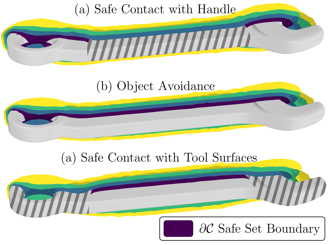
Figure 1: We implicitly define safe sets that consider the semantics of contact regions by introducing the semantics-aware distance. Its zero level set lies within the object, where contact with the surface is allowed, effectively generalizing the constraints defined as level sets of an object’s signed distance function. We visualize the semantics-aware distance of a combination wrench through its iso-surfaces – starting at the zero level set – which describes the safe set boundary. With our proposed computation method, query times are lower than $1\text{\,}\mathrm{\SIUnitSymbolMicro s}$ and render the function useful for control barrier function approaches to formally ensure the forward-invariance of the semantics-aware safe sets.

The goal of this paper is to extend the applicability of safety-related methods in robotic manipulation from collision avoidance towards the consideration of object affordances and semantics while performing and learning contact-rich manipulation tasks, by introducing the concept of a semantics-aware distance and an efficient numerical method to compute it.

The proposed method is simple and intuitively generalizes the safety approaches for collision avoidance based on distance functions. Let a function implicitly encode the safe set as the region of the domain that maps to non-negative values. While in collision avoidance applications the zero level-set coincides with the object’s surface, we lift this constraint and treat boundary values as variables, allowing the safe-set boundary to lie within or outside of the object’s surface, depending on the time-varying or configuration-dependent semantic state of the surface region, i.e., whether contact is allowed or not.

To obtain the semantics-aware distance function, we propose a computational method, using the Kelvin Transformation [1] to solve a Boundary Value Problem defined by the Laplace equation in the exterior of an object, and discretizing the Kelvin-Transformed domain through tetrahedralization. Our method also enables the computation of a global harmonic attractive field for guidance or autonomy, at marginally negligible computational and setup effort [29, 30, 31].

In validation experiments shown in Section V we evaluate the proposed computation method with respect to the formalized desirables presented in Section III. We further visualize the semantic-aware distance function through its iso-surfaces, an example harmonic guidance function in its exterior, and evaluate the method on a combination wrench, serving as a complex object. The paper concludes with comments on the limitations and applications of our approach in robotic manipulation.

II Preliminaries

II-A Linear PDE-based Distance Field Approximations

The homogeneous screened Poisson equation with Dirichlet boundary condition can be expressed as the boundary-value problem

$$u-c\Delta u=0\quad \mathrm{in}\quad\Omega$$

$$u=u_{\partial}\quad \mathrm{on}\quad\partial\Omega,$$ (1)

with Laplace operator $\Delta$, screening coefficient $c\in\mathbb{R}_{\geq 0}$, boundary function $u_{\partial}:\partial\Omega\to\mathbb{R}$, and solution $u:\Omega\cup\partial\Omega\to\mathbb{R}$, defined in the non-empty domain $\Omega\subset\mathbb{R}^{n}$ and its boundary $\partial\Omega$. The Laplace equation is the special case of the homogeneous screened Poisson equation in the limit as $c\rightarrow\infty$.

The solution $u$ of the screened Poisson equation

$$u-c\Delta u=0\quad \mathrm{in}\quad\Omega$$

$$u=1\quad \mathrm{on}\quad\partial\Omega,$$ (2)

is positive and differentiable in the domain interior, and has a maximum at the boundary. Using the negative logarithm transformation

$$w=-\sqrt{c}\,\mathrm{ln}(u)$$ (3)

the solution $u$ can be equivalently described as the solution $w$ to the regularized Eikonal equation

$$(1-|\nabla w|^{2})+\sqrt{c}\Delta w=0\quad \mathrm{in}\quad\Omega$$

$$w=0\quad \mathrm{on}\quad\partial\Omega.$$ (4)

As $c\rightarrow 0$, the solution $w$ approaches the exact distance-to-boundary function [32, 33, 34].

In bounded low-dimensional domains the equation can be effectively solved through numerical approaches, i.e., finite element and finite difference methods. One strategy to solve it in exterior or infinite domains is the Kelvin Transform, that leverages an inversion map to represent the infinite domain by a bounded domain [1].

II-B Kelvin Transformation for PDEs on Infinite Domains

To solve PDEs on infinite or unbounded domains, such as on the exterior of objects, the method of coordinate-stretching was introduced in the 70s, and treats the point of infinity through a “coordinate transformation of the infinite domain into a finite region” [35]. The Kelvin Transformation approach [1] fundamentally extends the coordinate-stretching approach by proposing to use the inversion map

$$\Phi(\mathbf{y})=\frac{\mathbf{y}}{|\mathbf{y}|^{2}},\quad\mathbf{y}\in\Omega_{\mathrm{inv}}\subset\mathbb{R}^{n}\setminus{\mathbf{0}}$$

$$\Phi^{-1}(\mathbf{x})=\frac{\mathbf{x}}{|\mathbf{x}|^{2}},\quad\mathbf{x}\in\Omega\subset\mathbb{R}^{n}\setminus{\mathbf{0}},$$ (5)

where $\Omega_{\mathrm{inv}}=\Phi^{-1}(\Omega)$, and decompose the solution $u(\mathbf{x})$ (or $U(\mathbf{y})$) into

$$u(\mathbf{x})=g(\mathbf{x})v(\mathbf{x})\quad\mathrm{or}\quad U(\mathbf{y})=G(\mathbf{y})V(\mathbf{y}),$$ (6)

where

1. the analytical behavior function $g(\mathbf{x})$ or its inverted counterpart $G(\mathbf{y})=g(\Phi(\mathbf{y}))$, captures the asymptotic behavior of the solution $u$ near infinity; and

2. the factor $v(\mathbf{x})$, or $V(\mathbf{y})=v(\Phi(\mathbf{y}))$, is to be solved numerically.

The change of variables from $U$ to $V$ removes the singularity at the inversion origin – otherwise present in coordinate stretching – such that the resulting PDE in the inverse domain extends to the compactified domain $\Omega_{\mathrm{inv}}\cup\{\mathbf{0}\}$ [1].

III Problem Statement

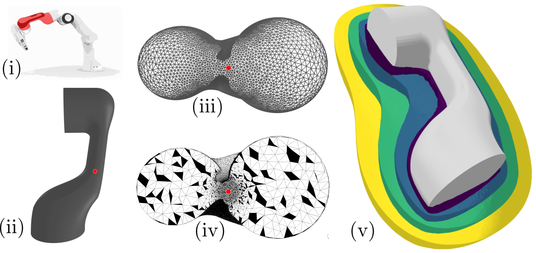
Figure 2: The computational method with the Kelvin Transformation approach is visualized in this figure, by using the 5th link of the Franka Robot (i) as an example object. The center of inversion is depicted as a red dot in insets (ii-iv). The inset (ii) shows the surface mesh of the object, (iii) shows the mesh transformed by the inversion map (5), (iv) shows the generated interior tetrahedral mesh, and (v) shows an iso-surface representation of the solution with constant boundary values. Corresponding numerical statistics are shown in Table II.

We introduce the notion of an object-wise semantics-aware distance function that implicitly defines safe sets for contact-rich manipulation tasks under consideration of time-varying task semantics, such as object affordances, task goals or user intent.

In this problem statement, we define the desirable characteristics that the semantics-aware distance function and its corresponding computation method should fulfill, in order to be useful for real-time control applications, e.g., to ensure the safety of actions commanded through teleoperation or from learned policies.

We focus on the case of a rigid object with finite non-empty interior $\Theta\subset\mathbb{R}^{3}$ and surface $\partial\Theta\subset\mathbb{R}^{2}$. A possibly time-varying semantic state $\sigma$ is defined on the object’s surface $\sigma:\partial\Theta\to\mathbb{R}$ and represents whether contact at a point on the object’s surface is allowed ($\sigma>0$) or not ($\sigma\leq 0$).

Let a function $h:\mathbb{R}^{3}\setminus\Theta\to\mathbb{R}$ implicitly describe the semantic-aware safe set $\mathcal{C}$ as the superlevel set

$$\mathcal{C} =\{\mathbf{x}\in\mathbb{R}^{3}\setminus\Theta\ |\ h(\mathbf{x})\geq 0\}$$ (7)

$$\partial\mathcal{C} =\{\mathbf{x}\in\mathbb{R}^{3}\setminus\Theta\ |\ h(\mathbf{x})=0\},$$ (8)

borrowing notation from Ames et al. [5]. The function $h$ encodes the semantic state $\sigma$ as a scaled signed distance between the zero level set of $h$ and a point on the object’s surface, i.e.,

$$h(\mathbf{x})=\gamma[d(\mathbf{x},\partial\mathcal{C})],\quad\sigma(\mathbf{x})-h(\mathbf{x})=0\quad\mathbf{x}\in\partial\Theta,$$ (9)

where $\gamma$ is a class $\mathcal{K}$ function, hence, the absolute value of the semantic function $\sigma$ is directly related to the allowed contact velocity, or to the distance margin. We call $h$ the semantics-aware distance function, and aim to use it to constrain the motion of points in the object’s exterior by the inequality constraint

$$\dot{h}(\mathbf{x})\geq\alpha[h(\mathbf{x})],\quad\mathbf{x}\in\mathbb{R}^{3}\setminus\Theta,$$ (10)

where $\alpha$ is a class $\mathcal{K}$ function, ensuring the forward-invariance of the safe set $\mathcal{C}$, under the condition that $h$ is continuously differentiable in the condition’s domain $\mathbb{R}^{3}\setminus\Theta$ [5].

We require the following properties from the computation method: (i) the computed function should adhere to the conditions (9), (ii) the memory requirements should be on par to those of signed distance functions ($\sim 1\,\mathrm{MB}$) to adequately function in standard robotic systems [10], (iii) the query times $t_{\mathrm{query}}$ should be substantially lower than $1\text{\,}\mathrm{ms}$ to achieve real-time control rates, and (iv) updates from a varying semantic state $\sigma$ should be considered online and require a update times $t_{\mathrm{solve}}\leq$33\text{\,}\mathrm{ms}$$.

IV Computation of Semantics-Aware Distances with the Kelvin Transformation

As described in the preliminaries, an exact distance function can be obtained by applying the negative logarithm transformation (3) to the solution of a screened Poisson equation with Dirichlet boundary condition, and we make use of the PDE formulation to represent the semantics-aware distance in the condition (9)

$$\sigma-\lim_{c\to 0}h_{\partial}=0\quad \mathrm{on}\quad\partial\Theta$$ (11)

$$\sigma+\lim_{c\to 0}\sqrt{c}\,\mathrm{ln}(u_{\partial})=0\quad \mathrm{on}\quad\partial\Theta$$ (12)

$$u_{\partial}=\lim_{c\to 0}\frac{1}{\sqrt{c}}\mathrm{exp}(-\sigma)\quad \mathrm{on}\quad\partial\Theta.$$ (13)

Instead of solving the exact screened Poisson equation in the limit as $c\rightarrow 0$, we propose to approximate the solution by the maximally regularized distance approximation, i.e., the solution of the Laplace equation with the vanishing condition at infinity

$$\Delta u=0\quad \mathrm{in}\quad\Theta$$

$$u=\mathrm{exp}(-\sigma)\quad \mathrm{on}\quad\partial\Theta$$

$$u\to 0\quad \mathrm{for}\quad|\mathbf{x}|\to\infty,$$ (14)

benefiting from the fact that the regularized approximation is exact at the boundary, ensuring the satisfaction of condition (9). The solution is also ensured to be smooth and free of extrema in the domain interior [31].

To solve the Laplace equation in infinite domains, such as in the exterior of an object, we turn to the Kelvin Transformation approach and define the sets

$$\Omega:=\mathbb{R}^{3}\setminus\Theta\cup\partial\Theta,\quad\partial\Omega:=\partial\Theta.$$ (15)

IV-A Solution with the Kelvin Transformation

We follow the approach presented by Nabizadeh et al. to solve Laplace equations through the Kelvin Transformation approach [1]. The computational method is depicted in Fig. 2. The analytical behavior function $G(\mathbf{y})$ – that captures the asymptotic behavior of the solution $u$ with the vanishing condition at infinity – for Laplace equations is

$$G(\mathbf{y})=|\mathbf{y}|,\quad\mathbf{y}\in\Omega_{\mathrm{inv}}\cup\{\mathbf{0}\}.$$ (16)

Using the inversion map (5) and the factorization (6), the exterior boundary value problem (14) can be exactly reformulated as

$$\Delta V(\mathbf{y})=0\quad \mathrm{in}\quad\Omega_{\mathrm{inv}}\cup\{\mathbf{0}\}$$

$$V(\mathbf{y})=V_{\partial}=\frac{U_{\partial}(\mathbf{y})}{G(\mathbf{y})}\quad \mathrm{on}\quad\partial\Omega_{\mathrm{inv}}$$ (17)

in the now bounded and compactified domain $\Omega_{\mathrm{inv}}\cup\{\mathbf{0}\}$, with $\Omega_{\mathrm{inv}}=\Phi^{-1}(\Omega)$ as presented in Section II-B.

The safety inequality constraint (10) requires the value and the time-derivative of the semantics-aware distance $h$, which is a function of the semantic state $\sigma$ and the evaluation point $\mathbf{x}$. Given that the frequency rate of the evaluation is orders of magnitude higher than the semantic state adaptation, we approximate the time derivative

$$\dot{h}=\nabla_{\mathbf{x}}h\dot{\mathbf{x}}+\nabla_{\sigma}h\dot{\sigma}\approx\nabla_{\mathbf{x}}h\dot{\mathbf{x}}+\cancel{\nabla_{\sigma}h\dot{\sigma}}$$ (18)

by assuming a relative quasi-static behavior of the semantic state. The gradient $\nabla_{\mathbf{x}}h$ is continuously differentiable in the exterior domain $\Omega$ and can be computed by the chain rule.

IV-B Linear Solver

Based on a tetrahedral-mesh approximation (with $N_{\mathrm{verts}}$ vertices and $N_{\mathrm{tets}}$ tetrahedrons) of the bounded domain $\Omega_{\mathrm{inv}}\cup\{\mathbf{0}\}$, we represent the matrix form of the vertex-wise Laplace operator as $\mathbf{L}\in\mathbb{R}^{N_{\mathrm{verts}}\times N_{\mathrm{verts}}}$, and introduce the matrix $\mathbf{A}\in\mathbb{R}^{N_{\mathrm{verts}}\times N_{\mathrm{verts}}}$ as the coefficient matrix.

This results in the following linear PDE expressed in the bounded domain

$$\mathbf{A}V=\mathbf{0}\quad \mathrm{in}\quad\Omega_{\mathrm{inv}}\cup\{\mathbf{0}\}$$

$$V=V_{\partial}\quad \mathrm{on}\quad\partial\Omega_{\mathrm{inv}},$$ (19)

with $\mathbf{A}=\mathbf{L}$ and $V$ as the vectorized vertex-wise solution.

The coefficient matrix $\mathbf{A}\in\mathbb{R}^{N_{\mathrm{verts}}\times N_{\mathrm{verts}}}$ is square and sparse. We reduce the linear system to solve only for the interior vertices, given that boundary values are known

$$\mathbf{b}_{\Omega} =-\mathbf{A}_{\Omega,\partial}V_{\partial}$$ (20)

$$\mathbf{A}_{\Omega,\Omega}V_{\Omega} =\mathbf{b}_{\Omega},$$ (21)

abusing notation with the $\Omega$ subscript representing the indices of vertices in the domain interior, and respectively $\partial$ analogue for vertices in the domain boundary.

The coefficient matrix can be factorized through an LU decomposition

$$\mathbf{L}_{\mathbf{A}}\mathbf{U}_{\mathbf{A}}=\mathbf{A}_{\Omega},$$ (22)

to efficiently compute the solution with varying boundary values – motivated by Crane et al. [34] – enabling the desired adaptive behavior of the semantics-aware distance function as encoded by the PDE solution.

IV-C Spatial Discretization

We choose to discretize the bounded domain with a tetrahedral volumetric mesh, given that it leads to a piecewise smooth approximation of the object’s surface and also allows for variable element sizing. We present the parametrization of the interior mesh generation, provide references to the definition of the differential operators employed, and describe the querying procedure.

IV-C1 Parametric Tetrahedralization

Ideally we want an interior mesh that is equivariant to the choice of inversion origin – we propose and leverage the following metric based sizing field to generate the interior mesh. A uniform mesh in the exterior domain is obtained by meshing the interior with

$$l_{\mathbf{y},\mathrm{nom}}(\mathbf{y})=|\mathbf{y}|^{2}l_{\mathbf{x}},\quad\mathbf{y}\in\Omega_{\mathrm{inv}}\cup\{\mathbf{0}\}$$ (23)

where $l_{\mathbf{x}}$ is the constant and nominal length-based element size in the exterior domain, and $l_{\mathbf{y}}(\mathbf{y})$ is the coordinate-dependent sizing field in the bounded domain, which are related by the Riemannian metric associated with the Kelvin Transformation [1].

The nominal interior sizing field (23) leads to an infinite density at the origin in the bounded domain. Given that the region of interest is near the surface, we set a lower bound for the sizing field, at the minimum sizing field value at the boundary of the interior domain $\partial\Omega_{\mathrm{inv}}$.

IV-C2 Differential Operators

Regarding differential operators, we make use of the vertex-wise Laplacian operator computed with the cotangent formula [36, 37] and the vertex-wise gradient operator as the volume-weighted average gradient on star. It is noteworthy that the resulting interpolated gradient within the tetrahedral mesh is continuously differentiable [38].

IV-C3 Value and Gradient Queries

The procedure to query a value at a given point in the exterior domain is described in Algorithm 1: (i) compute its inverse, (ii) find the enclosing tetrahedron, (iii) interpolate the vertex-wise interior solution $V$ from the enclosing tetrahedron, (iv) multiply by the behavior function $G$, and (v) transform through the negative logarithm map.

Algorithm 1 Query the Semantics-Aware Distance Function (14)

1:Solution $V$ of interior problem (19). Query point $\mathbf{x}\in\Omega$.

2:$\mathbf{y}\leftarrow\Phi^{-1}(\mathbf{x})$

3:$\tau\leftarrow\mathrm{locate}(\mathbf{y})$ $\triangleright$ Find enclosing tetrahedron $\tau$

4:$V(\mathbf{y})\leftarrow\mathrm{barycentricInterpolation}(\mathbf{y},\tau,V)$

5:$U(\mathbf{y})\leftarrow G(\mathbf{y})V(\mathbf{y})$

6:$h(\mathbf{x})\leftarrow-\mathrm{ln}[U(\mathbf{y})]$

7:return $h(\mathbf{x})$

The gradients are obtained analogue to the value query algorithm, computing the gradient $\nabla_{\mathbf{x}}h(\mathbf{x})$ after the barycentric interpolation of the numerical gradients.

V Validation

V-A Numerical Evaluation

In this experiment we aim to quantitatively assess whether the proposed method fulfills the requirements and desired characteristics as described in Sec. III.

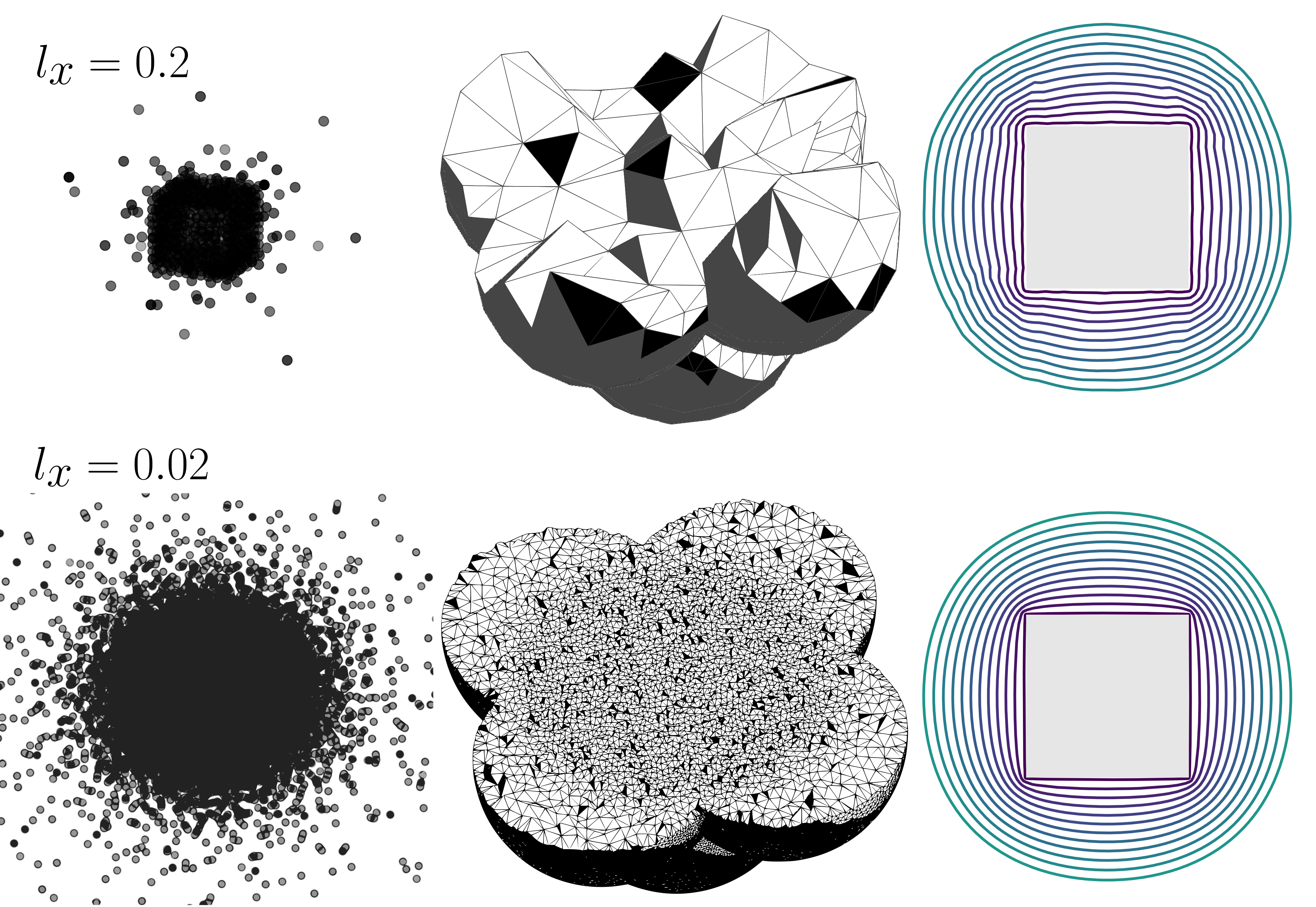
Figure 3: Visualization of the tested mesh range, as parametrized by the exterior domain length $l_{x}$. Top row: $l_{x}=0.2$, bottom row: $l_{x}=0.02$. The vertices are projected to the exterior domain through the inversion map 5, and shown in the left column. The mesh of the inverse domain is shown in the center. An iso-lines representation of the function evaluated in a grid of size $(1\,000\times 1\,000)$ within the cube $[-3,3]$ is shown in the right column.

TABLE I: Comparison of Size, Quality, and Computation time, evaluated as a function of varying mesh resolution. The mesh resolution is parametrized by the exterior length $l_{x}$, described in Section IV-C, and depicted in Fig. 3. The reported times for mesh, build, and decompose, are one-point estimates. The reported solve time is the mean of 100 evaluations. The reported query time is the median of a thousand points and using a cell hint. The RMSE is computed using the solution at 1M points in a planar grid and wrt. the solution obtained at $l_{x}=0.02$.

$l_{x}$	$N_{\mathrm{verts}}$	$N_{\mathrm{tets}}$	Size$/\mathrm{MB}$	$\mathrm{RMSE}_{l_{x}=0.02}$	$t_{\mathrm{mesh}}/$\text{\,}\mathrm{s}$$	$t_{\mathrm{build}}/$\text{\,}\mathrm{s}$$	$t_{\mathrm{decomp}}/$\text{\,}\mathrm{s}$$	$t_{\mathrm{solve}}/$\text{\,}\mathrm{ms}$$	$t_{\mathrm{query}}/$\text{\,}\mathrm{\SIUnitSymbolMicro s}$$
$0.02$	$157\,448$	$864\,083$	$38.0$	$-$	$12.4$	$1545$	$685.7$	$559.\pm 4.54$	$0.570$
$0.03$	$52\,865$	$273\,407$	$12.1$	$0.002$	$4.00$	$209.6$	$55.12$	$97.5\pm 1.18$	$0.414$
$0.04$	$24\,786$	$121\,965$	$5.6$	$0.004$	$1.82$	$43.32$	$9.140$	$28.6\pm 0.61$	$0.283$
$0.05$	$14\,124$	$66\,402$	$3.1$	$0.006$	$1.05$	$12.83$	$2.112$	$10.6\pm 0.37$	$0.279$
$0.06$	$8\,910$	$40\,610$	$1.8$	$0.009$	$0.68$	$4.256$	$0.801$	$5.31\pm 0.36$	$0.251$
$0.08$	$4\,415$	$18\,723$	$0.9$	$0.013$	$0.34$	$0.854$	$0.122$	$1.50\pm 0.21$	$0.217$
$0.10$	$2\,751$	$11\,109$	$0.5$	$0.018$	$0.22$	$0.333$	$0.048$	$0.63\pm 0.15$	$0.175$
$0.15$	$1\,132$	$4\,125$	$0.2$	$0.032$	$0.84$	$0.075$	$0.011$	$0.13\pm 0.04$	$0.211$
$0.20$	$615$	$2\,030$	$0.1$	$0.046$	$0.48$	$0.015$	$0.004$	$0.05\pm 0.01$	$0.116$

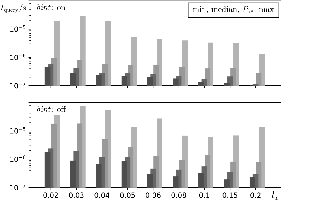
Figure 4: Comparison of query time statistics as a function of the mesh resolution parameter $l_{x}$, and the usage of a hint (warm start). In continuous motion, the hint can be set as the previous result (enclosing cell or tetra), and leads to query times considerably under a microsecond.

Given that our method is based on a numerical solution of the PDE (14), we measure the computation properties depending on the mesh resolution. In detail, we vary the parameter $l_{x}$ that determines the mesh generation process of the inverse or bounded domain, and measure method-characterizing size, quality, and performance related variables.

In this evaluation we use the cube as an example shape, leading to intuitive parametrizations, simple visualizations, and to study the behavior of the method in the presence of sharp edges. The inversion origin is placed at the center of the cube. All computations were performed on a single core (i7-8750H CPU @ $2.20\text{\,}\mathrm{GHz}$), implemented in C++, using the (standard) supernodal sparse LU factorization in Eigen [39]. The mesh generation and locate queries make use of the open source CGAL [40] implementations.

The range of tested mesh resolutions is visualized in Fig. 3, showing a subset of the vertices projected to the exterior domain, the generated interior mesh, and iso-lines of the resulting functions $h(u_{l_{x}})$ evaluated with boundary values $u_{\partial}=1$. Two expected behaviors become clear from the iso-line visualizations:

1. the numerical solution becomes smoother as the mesh becomes finer, and

2. the iso-lines approach the geometry of the boundary exactly (up to the mesh representation) as $h(u)\rightarrow 0$.

In addition to these qualitative observations, the numerical results of this evaluation are presented in Table I and Fig. 4.

The sizes of the evaluated models lie in the range ($0.1-38\,\mathrm{MB}$), which can be effectively managed by modern computing plarforms in robotic systems, thanks to the recent increases in memory availability and efficiency.

The quality of the solution should increase, as $l_{x}$ decreases. We evaluate and corroborate this expectation through a proxy measurement using the RMSE with respect to the solution computed at $l_{x}=0.02$.

The times for 3D mesh generation $t_{\mathrm{mesh}}$, constructing the sparse Laplace matrix operator $t_{\mathrm{build}}$, and computing the LU decomposition $t_{\mathrm{decomp}}$ are also shown in Table I. As stated above, all computations, were performed using a single CPU core, meaning that the time dedicated to preprocessing steps could be considerably reduced, e.g., by leveraging parallel algorithms to construct the Laplace operator.

The solving time is the main variable determining whether the method is capable of online-adaptive behavior. The solving times in the evaluated meshes lie in the range ($0.05-$559\text{\,}\mathrm{ms}$$), and are sufficiently low to enable online-recomputations of the solution, given that camera-based updates related to task level changes are generally streamed at a $30\text{\,}\mathrm{Hz}$ frequency, and could be processed by the tested models up to (incl.) $l_{x}=0.4$.

With CGAL tetrahedralizations we can use a hint or warm-start the locate query to find the enclosing tetrahedron given a point in the discretized domain. The effect of this hint on the query times is shown in Fig. 4. With and without the hint, the query times are more-than-sufficiently low ($0.5\text{\,}\mathrm{\SIUnitSymbolMicro s}$) for real-time applications. The usage of a hint leads to considerably faster queries, and is especially simple to leverage in continuous motion or point tracking problems. Because of the triangulation-walking nature of the query algorithm, relatively large query times can arise ($10\text{\,}\mathrm{\SIUnitSymbolMicro s}$), yet seldom, as shown in Fig. 4.

V-A1 Field Design

We showcase the effect of the semantic state $\sigma$ on the semantics-aware distance $h$ and of a guiding harmonic potential field using the following toy-example: allow contact on a face subset of a cube, and design a harmonic potential field with a unique minimum at the surface region where contact is allowed. We set a nominal $|\sigma|=0.1$ and its sign is determined by the semantic region. Similarly, the boundary values for the harmonic potential field are set to $u_{\partial}=1$ where $\sigma(\mathbf{x})\geq 0$ and $u_{\partial}=0.001$ otherwise. The length $l_{x}$ parametrizing the mesh generation is set to $0.05$.

The computed fields are shown in Fig. 5 through iso-lines in a planar evaluation, and in Fig. 6 by an iso-surface representation of the semantics-aware distance in 3D. In combination, the potential and safety fields enable globally attractive, reactive and safe navigation of points in the exterior domain, whereas a naive potential field based on euclidean distance could not consider the object’s geometry and would lead to a local minima on the opposite face of the cube even in this simple scenario.

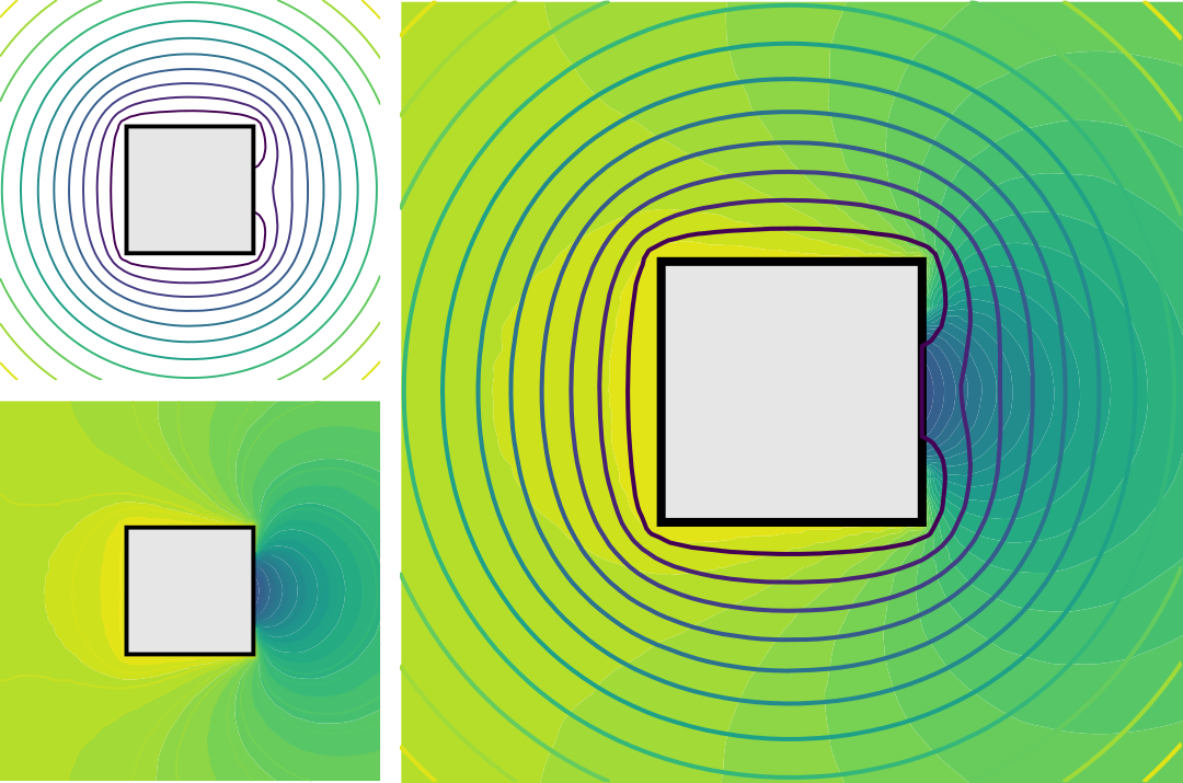
Figure 5: Planar evaluation of the semantics-aware distance (upper left inset), the harmonic potential field (lower left inset), and their superposed visualization (right inset). The safe set allows contact with a region of the cube’s right face, and the harmonic potential field globally attracts points through gradient descent (along the negative brightness gradient) to the safe contact region.

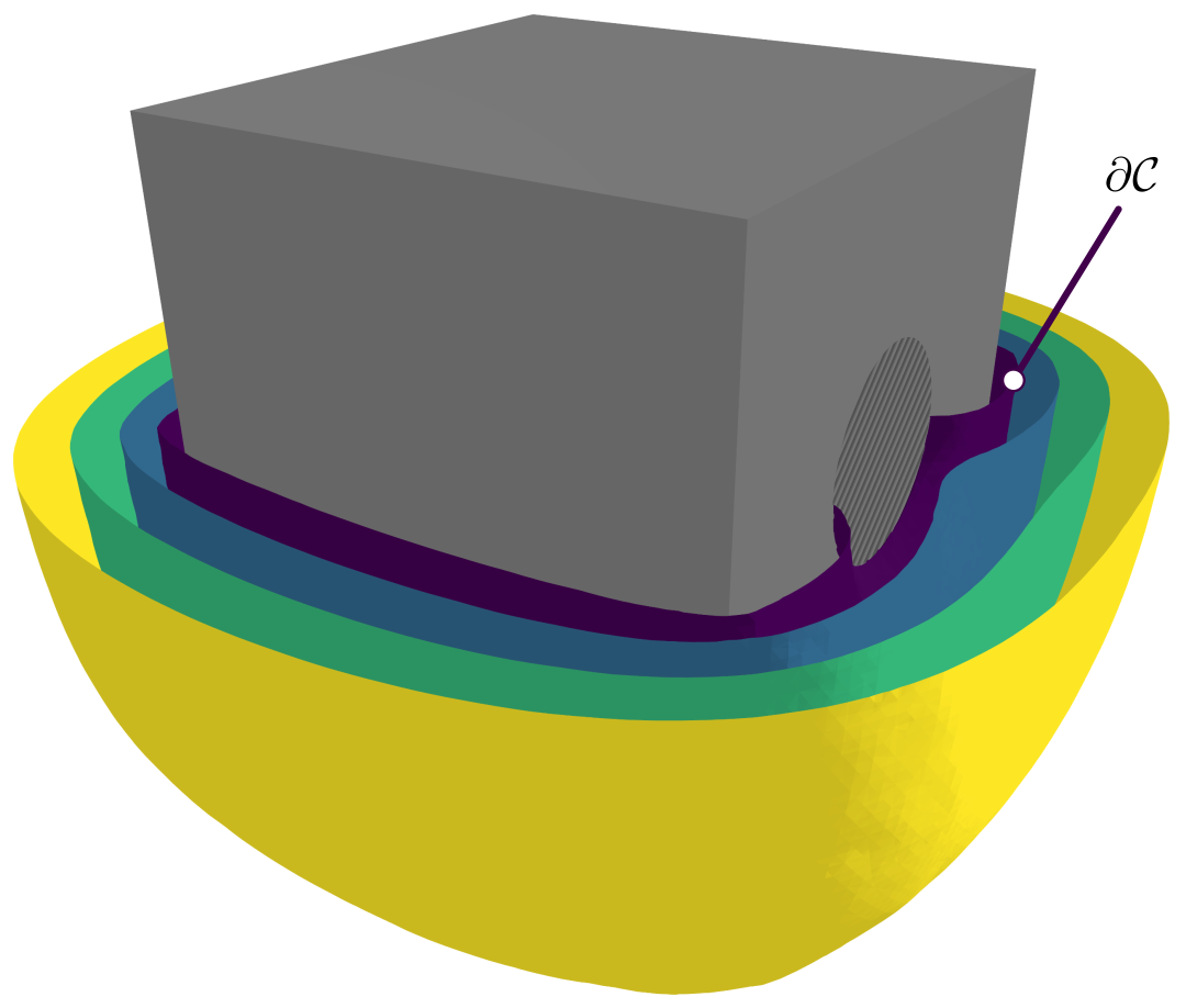
Figure 6: A qualitative visualization of the resulting semantic-aware distance through iso-surfaces within $[0,0.3]$ on the cube of side-length $l=2$. As designed through the semantic function $\sigma$ on the object’s surface $\partial\Theta$, contact with a face region (striped) of the cube is allowed, as shown by the surface-intersection zero level set $\partial\mathcal{C}$. The harmonic behavior of the solution is also demonstrated, by showing how the shape of iso-surfaces tend to a sphere as the semantic-distance increases.

Overall, the results from the presented numerical evaluation empirically support the theoretical motivation of the method, and suggest its applicability to real scenarios.

V-B Evaluation of the Semantic-Aware Distance on Complex Objects

We evaluate our method on a combination wrench, to (i) assess the performance of the method on a thin object that is also topologically distinct from a sphere, and (ii) visualize the encoding of semantics that are relevant to tool-based manipulation tasks. Given that the method is agnostic to the object’s geometry, we expect the results to directly generalize without any further changes in the parameters, apart from the object specific mesh generation.

The wrench has a length of $96.47\text{\,}\mathrm{mm}$. The length $l_{x,\mathrm{wrench}}$ parametrizing the mesh generation is set to $0.37\text{\,}\mathrm{mm}$ to accurately represent the surface geometry. Further, we set the inversion origin at the center of the wrench’s handle.

The numerical evaluation is shown in Table II. The performance lies within the expected ranges observed in the cube-based numerical evaluation in Section V-A. We take this observation as a strong empirical support for the geometry-independent behavior of the method.

TABLE II: Numerical Results of the Combination Wrench Evaluation. The columns are a subset of the ones in Table I and share their description.

Parameter	Comb. Wrench (Fig.1)	Franka Link 5 (Fig. 2)
$N_{\mathrm{verts}}$	$30\,749$	$37\,294$
$N_{\mathrm{tets}}$	$141\,546$	$215\,736$
Size$/\mathrm{MB}$	$7.2$	$8.4$
$t_{\mathrm{mesh}}/$\text{\,}\mathrm{s}$$	$3.68$	$2.201$
$t_{\mathrm{build}}/$\text{\,}\mathrm{s}$$	$69.03$	$100.2$
$t_{\mathrm{decomp}}/$\text{\,}\mathrm{s}$$	$2.16$	$33.46$
$t_{\mathrm{solve}}/$\text{\,}\mathrm{ms}$$	$14.6\pm 0.56$	$67.7\pm 1.32$
$t_{\mathrm{query}}/$\text{\,}\mathrm{\SIUnitSymbolMicro s}$$	$0.324$	$0.301$

Regarding the applications and varying semantics, we consider multiple usages of the tool depending on the allowed contact surfaces: (a) only contact with the handle is allowed, (b) any contact with the object should be avoided, and (c) only contact with the tool ends or functional surfaces is allowed. To this end, we parametrize the semantic state $\sigma(\mathbf{x})$ to be dependent on the point’s coordinate $z$ along the longitudinal axis $\mathbf{e}_{l}$ of the combination wrench. Concretely,

$$\sigma(\mathbf{x})=\mathrm{tanh}(\mathrm{abs}(\mathbf{e}_{l}^{T}\mathbf{x})-d_{0}))\sigma_{\mathrm{nom}},$$ (24)

where $\sigma_{\mathrm{nom}}$ is a nominal constant semantic value, and $d_{0}\in\mathbb{R}_{\geq 0}$ represents the symmetric location of the transition between semantic regions. We implement the cases (a)-(c) listed above: (a) $\sigma_{\mathrm{nom}}=-0.05$, $d_{0}=25$, (b) $\sigma(\mathbf{x})=0.05$, and (c) $\sigma_{\mathrm{nom}}=0.05$, $d_{0}=25$. The resulting functions are visualized through iso-surfaces in Fig. 1, and match the designed safe sets.

VI Conclusion

We introduce the semantics-aware distance and propose a numerical method to compute it, enabling safe reactive behavior while adaptively considering regional contact constraints in contact-rich manipulation tasks.

The proposed method generalizes the applicability of safety-related methods in robotic manipulation from collision avoidance towards the consideration of object affordances and semantics while performing and learning contact-rich manipulation tasks.

While the semantics-aware distance is independent of the method used to obtain it, a limitation of our method is the assumption that the objects are of known geometry and provided in a mesh-based representation. Our computational method, based on the Kelvin Transformation, applies therefore to interactions with known objects, which are still ubiquitous in robotic manipulation tasks. Further, although the solutions of the Laplace equation are smooth in the domain interior, our finite-element discretization results instead in piecewise-smooth solutions.

These two limitations lead to interesting and relevant extensions of the method: developing the method to consider unknown objects, and approximating solutions through analytical basis functions.

The sub-microsecond query times and the continuously differentiable gradients of the function motivate promising applications, especially within planning and trajectory optimization for whole-body manipulation tasks, not only from a safety perspective but also by leveraging harmonic potential fields for globally-informed guidance.

References

- [1] Mohammad Sina Nabizadeh, Ravi Ramamoorthi, and Albert Chern. Kelvin transformations for simulations on infinite domains. ACM Trans. Graph., 40(4):97–1, 2021.
- [2] Daniel Kappler, Franziska Meier, Jan Issac, Jim Mainprice, Cristina Garcia Cifuentes, Manuel Wüthrich, Vincent Berenz, Stefan Schaal, Nathan Ratliff, and Jeannette Bohg. Real-time perception meets reactive motion generation. IEEE Robotics and Automation Letters, 3(3):1864–1871, 2018.
- [3] Oussama Khatib. Real-time obstacle avoidance for manipulators and mobile robots. The international journal of robotics research, 5(1):90–98, 1986.
- [4] Daniel E Koditschek and Elon Rimon. Robot navigation functions on manifolds with boundary. Advances in applied mathematics, 11(4):412–442, 1990.
- [5] Aaron D Ames, Samuel Coogan, Magnus Egerstedt, Gennaro Notomista, Koushil Sreenath, and Paulo Tabuada. Control barrier functions: Theory and applications. In 2019 18th European control conference (ECC), pages 3420–3431. IEEE, 2019.
- [6] Murilo Marques Marinho, Bruno Vilhena Adorno, Kanako Harada, and Mamoru Mitsuishi. Dynamic active constraints for surgical robots using vector-field inequalities. IEEE Transactions on Robotics, 35(5):1166–1185, 2019.
- [7] Karl Van Wyk, Mandy Xie, Anqi Li, Muhammad Asif Rana, Buck Babich, Bryan Peele, Qian Wan, Iretiayo Akinola, Balakumar Sundaralingam, Dieter Fox, Byron Boots, and Nathan D. Ratliff. Geometric fabrics: Generalizing classical mechanics to capture the physics of behavior. IEEE Robotics and Automation Letters, 7(2):3202–3209, 2022.
- [8] Mikhail Koptev, Nadia Figueroa, and Aude Billard. Neural joint space implicit signed distance functions for reactive robot manipulator control. IEEE Robotics and Automation Letters, 8(2):480–487, 2022.
- [9] Puze Liu, Kuo Zhang, Davide Tateo, Snehal Jauhri, Jan Peters, and Georgia Chalvatzaki. Regularized deep signed distance fields for reactive motion generation. In 2022 IEEE/RSJ International Conference on Intelligent Robots and Systems (IROS), pages 6673–6680. IEEE, 2022.
- [10] Yiming Li, Yan Zhang, Amirreza Razmjoo, and Sylvain Calinon. Learning robot geometry as distance fields: Applications to whole-body manipulation. arXiv preprint arXiv:2307.00533, 2023.
- [11] Ante Marić, Yiming Li, and Sylvain Calinon. Online learning of piecewise polynomial signed distance fields for manipulation tasks. arXiv preprint arXiv:2401.07698, 2024.
- [12] Bernhard P Graesdal, Shao YC Chia, Tobia Marcucci, Savva Morozov, Alexandre Amice, Pablo A Parrilo, and Russ Tedrake. Towards tight convex relaxations for contact-rich manipulation. arXiv preprint arXiv:2402.10312, 2024.
- [13] Adam Heins and Angela P Schoellig. Force push: Robust single-point pushing with force feedback. arXiv preprint arXiv:2401.17517, 2024.
- [14] Igor Mordatch, Zoran Popović, and Emanuel Todorov. Contact-invariant optimization for hand manipulation. In Proceedings of the ACM SIGGRAPH/Eurographics symposium on computer animation, pages 137–144, 2012.
- [15] Tom Erez and Emanuel Todorov. Trajectory optimization for domains with contacts using inverse dynamics. in 2012 ieee. In RSJ International Conference on Intelligent Robots and Systems, pages 4914–4919.
- [16] Ben Burgess-Limerick, Jesse Haviland, Chris Lehnert, and Peter Corke. Reactive base control for on-the-move mobile manipulation in dynamic environments. IEEE Robotics and Automation Letters, 2024.
- [17] Danny Driess, Jung-Su Ha, Marc Toussaint, and Russ Tedrake. Learning models as functionals of signed-distance fields for manipulation planning. In Conference on robot learning, pages 245–255. PMLR, 2022.
- [18] Leon Sievers, Johannes Pitz, and Berthold Bäuml. Learning purely tactile in-hand manipulation with a torque-controlled hand. In 2022 International Conference on Robotics and Automation (ICRA), pages 2745–2751. IEEE, 2022.
- [19] Aravind Rajeswaran, Vikash Kumar, Abhishek Gupta, Giulia Vezzani, John Schulman, Emanuel Todorov, and Sergey Levine. Learning complex dexterous manipulation with deep reinforcement learning and demonstrations. arXiv preprint arXiv:1709.10087, 2017.
- [20] Cheng Chi, Siyuan Feng, Yilun Du, Zhenjia Xu, Eric Cousineau, Benjamin Burchfiel, and Shuran Song. Diffusion policy: Visuomotor policy learning via action diffusion. arXiv preprint arXiv:2303.04137, 2023.
- [21] Mengchao Zhang, Jose Barreiros, and Aykut Ozgun Onol. Plan-guided reinforcement learning for whole-body manipulation. arXiv preprint arXiv:2310.12263, 2023.
- [22] Mia Kokic, Johannes A Stork, Joshua A Haustein, and Danica Kragic. Affordance detection for task-specific grasping using deep learning. In 2017 IEEE-RAS 17th International Conference on Humanoid Robotics (Humanoids), pages 91–98. IEEE, 2017.
- [23] Maozhen Wang, Rui Luo, Aykut Özgün Önol, and Taşkin Padir. Affordance-based mobile robot navigation among movable obstacles. In 2020 IEEE/RSJ International Conference on Intelligent Robots and Systems (IROS), pages 2734–2740. IEEE, 2020.
- [24] Boyang Ti, Yongsheng Gao, Jie Zhao, and Sylvain Calinon. An optimal control formulation of tool affordance applied to impact tasks. IEEE Transactions on Robotics, 40:1966–1982, 2024.
- [25] Yiran Geng, Boshi An, Haoran Geng, Yuanpei Chen, Yaodong Yang, and Hao Dong. Rlafford: End-to-end affordance learning for robotic manipulation. In 2023 IEEE International Conference on Robotics and Automation (ICRA), pages 5880–5886. IEEE, 2023.
- [26] Jakob Thumm and Matthias Althoff. Provably safe deep reinforcement learning for robotic manipulation in human environments. In 2022 International Conference on Robotics and Automation (ICRA), pages 6344–6350. IEEE, 2022.
- [27] Puze Liu, Kuo Zhang, Davide Tateo, Snehal Jauhri, Zhiyuan Hu, Jan Peters, and Georgia Chalvatzaki. Safe reinforcement learning of dynamic high-dimensional robotic tasks: navigation, manipulation, interaction. In 2023 IEEE International Conference on Robotics and Automation (ICRA), pages 9449–9456. IEEE, 2023.
- [28] Hanna Krasowski, Jakob Thumm, Marlon Müller, Lukas Schäfer, Xiao Wang, and Matthias Althoff. Provably safe reinforcement learning: Conceptual analysis, survey, and benchmarking. Transactions on Machine Learning Research, 2023.
- [29] Christopher I Connolly, J Brian Burns, and Rich Weiss. Path planning using laplace’s equation. In Proceedings., IEEE International Conference on Robotics and Automation, pages 2102–2106. IEEE, 1990.
- [30] Hans Jacob S Feder and J-JE Slotine. Real-time path planning using harmonic potentials in dynamic environments. In Proceedings of International Conference on Robotics and Automation, volume 1, pages 874–881. IEEE, 1997.
- [31] Jin-Oh Kim and Pradeep Khosla. Real-time obstacle avoidance using harmonic potential functions. 1992.
- [32] Alexander G Belyaev and Pierre-Alain Fayolle. On variational and pde-based distance function approximations. In Computer Graphics Forum, volume 34, pages 104–118. Wiley Online Library, 2015.
- [33] Karthik S Gurumoorthy and Anand Rangarajan. A schrödinger equation for the fast computation of approximate euclidean distance functions. In International Conference on Scale Space and Variational Methods in Computer Vision, pages 100–111. Springer, 2009.
- [34] Keenan Crane, Clarisse Weischedel, and Max Wardetzky. Geodesics in heat: A new approach to computing distance based on heat flow. ACM Transactions on Graphics (TOG), 32(5):1–11, 2013.
- [35] Chester E Grosch and Steven A Orszag. Numerical solution of problems in unbounded regions: coordinate transforms. Journal of Computational Physics, 25(3):273–295, 1977.
- [36] Marc Alexa, Philipp Herholz, Maximilian Kohlbrenner, and Olga Sorkine-Hornung. Properties of laplace operators for tetrahedral meshes. In Computer Graphics Forum, volume 39, pages 55–68. Wiley Online Library, 2020.
- [37] Keenan Crane. The n-dimensional cotangent formula. Online note. URL: https://www. cs. cmu. edu/~ kmcrane/Projects/Other/nDCotanFormula. pdf, pages 11–32, 2019.
- [38] Claudio Mancinelli, Marco Livesu, and Enrico Puppo. A comparison of methods for gradient field estimation on simplicial meshes. Computers & Graphics, 80:37–50, 2019.
- [39] Gaël Guennebaud, Benoît Jacob, et al. Eigen v3. http://eigen.tuxfamily.org, 2010.
- [40] The CGAL Project. CGAL User and Reference Manual. CGAL Editorial Board, 5.6.1 edition, 2024.