Bayesian WeakS-to-Strong
from Text Classification to Generation

Abstract

Advances in large language models raise the question of how alignment techniques will adapt as models become increasingly complex and humans will only be able to supervise them weakly. Weak-to-Strong mimics such a scenario where weak model supervision attempts to harness the full capabilities of a much stronger model. This work extends Weak-to-Strong to WeakS-to-Strong by exploring an ensemble of weak models which simulate the variability in human opinions. Confidence scores are estimated using a Bayesian approach to guide the WeakS-to-Strong generalization. Furthermore, we extend the application of WeakS-to-Strong from text classification tasks to text generation tasks where more advanced strategies are investigated for supervision. Moreover, direct preference optimization is applied to advance the student model’s preference learning, beyond the basic learning framework of teacher forcing. Results demonstrate the effectiveness of the proposed approach for the reliability of a strong student model, showing potential for superalignment.

1 Introduction

With the increase in computing power and the amount of training data available, the capabilities of large language models (LLMs) have been continuously brought closer to humans in many aspects. Despite their impressive performance, the preferences and values of pre-trained LLMs do not always align with humans, and dedicated approaches are needed to tackle the problem. Based on large-scale instruction datasets, supervised finetuning (SFT) encourages LLMs to follow human instructions more strictly and respond more safely [28]. Reinforcement learning (RL) is commonly applied to such alignment. By collecting model output values and the corresponding human feedback, the model can be finetuned by RL to avoid generating undesirable outputs [33, 3, 18, 17, 1].

Since no current model has surpassed human intelligence yet, existing alignment methods, such as SFT and RL from human feedback (RLHF), remain effective. However, it is worthwhile considering future scenarios where artificial intelligence (AI) might surpass human intelligence in all aspects. Would the current alignment methods still be effective for such super AI models? How could humans supervise the super AI? To simulate this future scenario, an analogy situation is designed that downgrades both sides: using a weak model to simulate humans and a strong model to simulate future super AI [7], which is termed as superalignment. It has been demonstrated that adding a simple auxiliary loss can achieve effective Weak-to-Strong generalization, even if the weak model’s supervision contains many errors, which offers hope of achieving superalignment. Nonetheless, this is just the beginning of exploring along the path of Weak-to-Strong.

This paper extends the discussion on Weak-to-Strong in two directions. First, given the inherent capability gap between the weak model and the strong model, we propose using an ensemble of multiple weak models to improve the quality of weak supervision, which is called WeakS-to-Strong. This also accounts for the scenario where human opinions might diverge in tasks without a commonly accepted standard. Several approaches have been studied to effectively leverage the diversity of different weak models, and we adapt a Bayesian approach referred to as evidential deep learning (EDL) [24] to better estimate broader human preferences by learning a prior distribution over the weak labels produced by the weak models. Furthermore, the Weak-to-Strong task was primarily studied for text classification tasks [7]. This paper extends the scope to text generation tasks and demonstrates that the proposed Bayesian WeakS-to-Strong approach is effective for both. To better align with human preferences, a variant of direct preference optimization (DPO) [22] called conservative DPO (cDPO) [9] is used to finetune the strong model further on RL principles.

Our main contributions are summarized as follows.

• We proposed Bayesian WeakS-to-Strong which largely improves the quality of weak supervision and recovers the performance of the strong model.

• We propose to generalize both Weak-To-Strong and WeakS-to-Strong from text classification to generation tasks, extending their scope from content regulation to content generation.

• When applied to text generation, a token-level confidence measure is proposed to achieve soft labels for strong model training. We also propose the modified DPO algorithm under the Bayesian WeakS-to-Strong framework to further improve text generation performance.

2 Related Work

AI Alignment. Aligning LLMs with human preferences has been a long-standing goal. Instruction tuning uses extensive datasets to improve LLMs’ adherence to human instructions [28]. RL allows LLMs to learn what types of responses humans prefer or dislike, with proximal policy optimization (PPO) being an effective RL method first applied to LLMs and becoming part of the standard RLHF process [33, 3, 18, 17, 1]. However, PPO training can be unstable, leading to the development of DPO [22]. Due to the high cost of obtaining human preference data, there is now exploration into using LLMs to simulate human preferences, provide feedback, and finetune models [13, 4, 10].

Variability in Human Opinions. In the process of aligning AI with human preferences, it is important to consider the inconsistency of human preferences [14], which often leads to multi-label problems. Previously, many approaches used simple methods like voting, aggregation, and averaging to handle multi-labels [8, 16, 19, 20]. However, these methods do not effectively capture the preference differences of individual annotators included in the multiple labels. To better estimate the diversity of human preferences, Bayesian principles have been introduced. Deep neural network models can be used to predict prior distributions, which are considered to produce the multiple available labels to estimate a broader range of human preferences [24, 31, 30].

Weak-to-Strong. The goal of Weak-to-Strong is to use a weak model to better supervise a strong model. OpenAI demonstrated that adding auxiliary confidence loss from the strong model itself can significantly improve the Weak-to-Strong performance [7]. Following OpenAI’s work, several studies emerged to introduce multiple weak models, used either in series or parallel, to improve the quality of supervision provided by the weak models [15, 23]. In addition, confidence scores are incorporated to help the strong model assess the supervision quality provided by the weak models [11] and weak model can be directly used to modify the output of the strong model [12].

3 WeakS-to-Strong Methodology

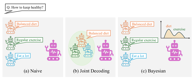
Figure 1: An overview diagram of the three ensemble approaches: (a) Naive multi-weak, (b) Joint decoding, and (c) Bayesian multi-weak.

3.1 Preliminary: Weak-to-Strong

The Weak-to-Strong pipeline [7] involves three steps: (i) create a weak supervisor by finetuning a small pre-trained model on ground-truth labels; (ii) train a strong student model $\boldsymbol{f_{\Lambda}}$ with weak supervision by finetuning a pre-trained LLM using “weak labels” generated by weak supervisors, where $\boldsymbol{\Lambda}$ is the parameters of the strong model; (iii) finetune the large pre-trained model directly using ground-truth labels which serves as the ceiling.

To leverage the superior generalization capabilities and prior knowledge of strong model, a loss function with auxiliary confidence loss is proposed [7]:

$$\mathcal{L}=(1-\gamma)*\operatorname{CE}(\boldsymbol{f_{\Lambda}}(\boldsymbol{x}),\boldsymbol{y}_{w})+\gamma*\operatorname{CE}(\boldsymbol{f_{\Lambda}}(\boldsymbol{x}),\boldsymbol{\hat{f}_{\Lambda}}(\boldsymbol{x}))$$ (1)

where $\boldsymbol{y}_{w}$ represents the weak label from weak model, $\boldsymbol{\hat{f}_{\Lambda}}(\boldsymbol{x})$ refers to the predicted class of strong model given input $\boldsymbol{x}$, and $\operatorname{CE}(\cdot,\cdot)$ denotes the cross-entropy loss. The second term is an (optional) auxiliary self-training loss designed to increase the confidence of the strong model to itself. The weight of the second loss, $\gamma$, linearly grows up from 0 to a pre-defined hyper-parameter $\gamma_{\text{max}}$, which gradually reduces the weight on the weak labels and increase the weight on self-training when the number of training step increases.

3.2 Extending Weak-to-Strong with multiple weak models

Although it has been shown that the Weak-to-Strong approach can recover part of the strong model’s performance [7], the errors in weak labels limit the performance of Weak-to-Strong generalization. In response to this problem, we propose to leverage the complementarity of the error patterns of multiple weak models using the ensemble strategy, which is referred to as WeakS-to-Strong.

A naive approach to implementing an ensemble of multiple weak models is to calculate the loss for each weak label respectively and then average these losses. An improvement of this approach is to take a weighted sum instead of a simple average:

$$\mathcal{L}_{\text{Naive}}=\sum_{i=1}^{N}w_{i}\operatorname{CE}(\boldsymbol{f_{\Lambda}}(\boldsymbol{x}),\boldsymbol{y}_{w}^{(i)})),$$ (2)

where $N$ is the number of weak models, $\boldsymbol{y}_{w}^{(i)}$ is the $i$th weak label produced by the $i$th weak model, and $w_{i}$ is a pre-defined weight of the loss regarding the the $i$th weak model. This approach is referred to as a naive multi-weak system in the rest of the paper.

3.3 Bayesian WeakS-to-Strong

For superalignment, multiple weak models are used to mimic the subjective preferences of multiple humans, which can be considered as observations drawn from an underlying distribution of the opinions of all humans. The naive approach described in Section 3.2 solely relies on these observations. The number of observations (human annotations or weak labels) is often very limited due to the considerable cost of hiring a new human annotator or training a new weak model. Such a limited number of observations may not result in a good approximation of the true human opinion distribution. Having biased preferences or values is particularly unacceptable in the safety domain and can cause a failure of superalignment. Therefore, we propose a Bayesian WeakS-to-Strong approach based on EDL [24] to estimate the human opinion distribution based on the weak labels. Figure 1(c) illustrates the framework where three weak models are involved.

Consider a weak label from the $i^{th}$ weak model $\boldsymbol{y}_{w}^{(i)}$, which is a one-hot vector with $y_{w}^{(i,k)}$ being one if it belongs to class $k$ and zero otherwise. $\boldsymbol{y}_{w}^{(i)}$ is sampled from a categorical distribution (of the labels of weak models) $\text{Cat}(\boldsymbol{\pi})$, where each component ${\pi}_{k}$ corresponds to the probability assignment over the possible classes $\boldsymbol{y}_{w}^{(i)}\sim\mathrm{P}(\boldsymbol{y}|\boldsymbol{\pi})=\operatorname{Cat}(\boldsymbol{\pi}).$ EDL places a Dirichlet prior over the categorical distribution representing the probability of each categorical probability assignment, hence modelling second-order probability $\boldsymbol{\pi}\sim\mathrm{p}(\boldsymbol{\pi}|\boldsymbol{\alpha})$, where $\boldsymbol{\alpha}$ is the hyperparameter of the Dirichlet prior. The strong model $\boldsymbol{f_{\Lambda}}$ is trained to predict $\boldsymbol{\alpha}$ for each input by minimizing the negative log-likelihood of sampling $\boldsymbol{y}_{w}^{(i)}$ given the predicted Dirichlet prior:

$$\mathcal{L}_{\text{NLL}}^{(i)}=-\log\int\mathrm{P}(\boldsymbol{y}_{w}^{(i)}|\boldsymbol{\pi})\mathrm{p}(\boldsymbol{\pi}|\boldsymbol{\alpha})\mathrm{d}\boldsymbol{\pi}=\sum_{k=1}^{K}y_{w}^{(i,k)}(\log(\alpha_{0})-\log(\alpha_{k})),$$ (3)

where $K$ is the number of classes, $\alpha_{0}=\sum_{k=1}^{K}\alpha_{k}$ is the Dirichlet strength, and $y_{w}^{(i,k)}$ is the $k^{th}$ value of label $\boldsymbol{y}_{w}^{(i)}$. Following [24], a regularization term $\mathcal{L}_{\text{REG}}^{(i)}$ (see Appendix B for details) is added to calibrate uncertainty estimation, resulting in the EDL loss $\mathcal{L}_{\text{EDL}}^{(i)}=\mathcal{L}_{\text{NLL}}^{(i)}+\lambda_{\text{EDL}}\mathcal{L}_{\text{REG}}^{(i)}$ where $\lambda_{\text{EDL}}$ is the coefficient.

Apart from the class predicted by the weak models, the confidence of weak models is also incorporated for better distribution estimation. Let $(p_{1}^{(i)},\dots,p_{K}^{(i)})$ be the probability assignment predicted by the $i^{th}$ weak model, the EDL loss for each class is calculated based on the predicted probability assignment for each weak model and then combined in the same way as in Eqn. (2). That is,

$$\mathcal{L}_{\text{EDL}}(\boldsymbol{f_{\Lambda}}(\boldsymbol{x}),\{\boldsymbol{y}_{w}^{(i)}\}_{i=1}^{N})=\sum_{i=1}^{N}w_{i}\sum_{k=1}^{K}p_{k}\mathcal{L}_{\text{EDL}}^{(i)}(\boldsymbol{f_{\Lambda}}(\boldsymbol{x}),\hat{\boldsymbol{y}}_{w}^{(i)}))$$ (4)

where $\hat{\boldsymbol{y}}_{w}^{(i)}$ is the predicted class, and $w_{i}$s are hyperparameters set to the same values as used in the Naive multi-weak approach. As a result, the auxiliary confidence loss described in Eqn. (1) is adapted for Bayesian WeakS-to-Strong as follows:

$$\mathcal{L}=(1-\gamma)*\mathcal{L}_{\text{EDL}}(\boldsymbol{f_{\Lambda}}(\boldsymbol{x}),\{\boldsymbol{y}_{w}^{(i)}\}_{i=1}^{N})+\gamma*\mathcal{L}_{\text{EDL}}(\boldsymbol{f_{\Lambda}}(\boldsymbol{x}),\boldsymbol{\hat{f}_{\Lambda}}(\boldsymbol{x})).$$ (5)

In the term of $\mathcal{L}_{\text{EDL}}(\boldsymbol{f_{\Lambda}}(\boldsymbol{x}),\boldsymbol{\hat{f}_{\Lambda}}(\boldsymbol{x}))$, the class index predicted by the strong model $\boldsymbol{\hat{f}_{\Lambda}}(\boldsymbol{x})$ is used as the target. That is to say, the predictions of the strong student model are applied as part of the distribution estimation along with the weak label.

4 WeakS-to-Strong for Sequence Generation

4.1 Label Formulation via Joint-Decoding

To enable the strong model to directly generate trustworthy content rather than only being trained to understand whether the content is trustworthy or not, we propose to extend the scope of Weak-to-Strong from text classification to text generation. We also propose to jointly decode with multiple weak models to derive the sequence-level training target of the strong model. In contrast to the Naive multi-weak scheme, joint decoding employs multiple weak models to collaboratively determine one single target, reducing the risk of the strong model being affected by the potential biases that exist in the label space of the separate weak models.

Specifically in this paper, we perform joint decoding in a re-ranking fashion. For each weak model, the top $M$ output sequences are generated by beam search in decoding. We gather the output sequences from the $N$ weak models to form a list of $M\times N$ sequences. Next, for each sequence, $N$ scores are computed by generating it using each weak model separately (via teacher forcing) and aggregating the output (log-)probabilities. We perform a weighted sum of the $N$ scores as the final score assigned to each sequence, where the same set of weights is fixed within each task. The sequence with the highest final score will be used as the target sequence for strong model training. That is,

$$\boldsymbol{y}^{(i)}_{w}=\operatorname*{argmax}_{m}\mathrm{P}(\boldsymbol{y}^{(i)}_{w}(m))=\operatorname*{argmax}_{m}\sum_{i=1}^{N}\lambda_{i}\mathrm{P}(\boldsymbol{y}^{(i)}_{w}(m)|\theta_{i}),$$ (6)

where $\boldsymbol{y}^{(i)}_{w}(m)$ is the $m$th output sequence, $\lambda_{i}$ is the weight assigned to the $i$th weak model, $\theta_{i}$ represents model parameters of the $i$th weak model, and $m\in[1,M\times N]\cap\mathbb{Z}$.

4.2 Confidence measure for weak sequence labels

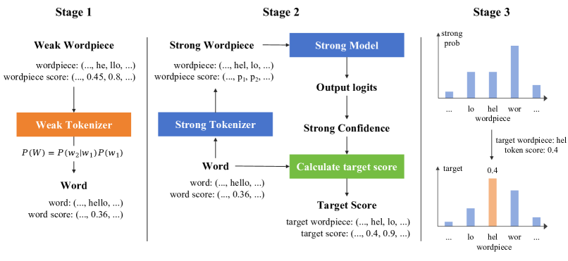
Figure 2: The process of transforming per-token confidence scores from the sequence tokenized by the weak model to the sequence tokenized by the strong. The word “hello” is used as an example. Stage 1: The words and word scores are obtained from the weak model wordpieces and their scores. Stage 2: The words are tokenized by the strong model tokenizer, and the tokenized sequences are fed into the strong model to obtain the strong model predicted probability (denoted as confidence) for each token $s_{i}$. This probability is used to split word scores into target wordpiece probabilities $P(s_{i})$ while keeping the probability of the word unchanged. Stage 3: The obtained target score is transformed into the soft label by scaling the strong output distribution using $P(s_{i})$.

The key challenge of directly applying the Weak-to-Strong loss [7] to the sequence generation task is the token-level soft labelling for the target sequence. As the tokenizers are different between the weak and the strong models, it is infeasible to obtain a one-to-one mapping from weak model output distributions to each token in the target sequence.

To obtain the soft label $\boldsymbol{y}_{w}$ for the strong model using weak model output probabilities and bridge the gap caused by different tokenizers, we use words as an intermediary. Figure 2 shows an example of the process in three stages. In stage 1, the per-token output probabilities of the weak models are obtained when generating output sequences. The probabilities of wordpieces in a word, referred to as wordpiece scores, are then multiplied together to obtain the score of word $W$. In stage 2, the word score is used to assign probabilities to tokens from the strong model tokenizer, following Eqn. (7).

$$\mathrm{P}(W)=\mathrm{P}(w_{2}|w_{1})\mathrm{P}(w_{1})=\mathrm{P}(s_{2}|s_{1})\mathrm{P}(s_{1}),$$ (7)

where we use a word containing two wordpieces from both weak and strong tokenizers as an example, and $w_{1},w_{2}$ and $s_{1},s_{2}$ are both token strings that can form $W$, which are generated by the tokenizers of the weak and strong models respectively. To obtain the actual assignment of scores to each strong model token $s_{i}$, instead of assigning equal probabilities to all tokens involved, we compute a weight from the strong model confidence when predicting $s_{1}$ and $s_{2}$ to approximate the decomposition by

$$\mathrm{P}(s_{1})=\frac{e^{C_{s}(s_{1})}}{e^{C_{s}(s_{1})}+e^{C_{s}(s_{2})}}\mathrm{P}(W),\qquad\mathrm{P}(s_{2})=\frac{e^{C_{s}(s_{2})}}{e^{C_{s}(s_{1})}+e^{C_{s}(s_{2})}}\mathrm{P}(W),$$ (8)

where $C_{s}(s_{i})$ is strong model confidence at the step predicting wordpiece $s_{i}$, which is the maximum probability in the strong model output distribution at that step in practice. In this way, smaller target confidence scores are allocated to tokens with lower strong model confidence (i.e., harder to predict), while larger confidence scores are allocated to tokens with higher strong model confidence.

After obtaining the probability of the target token of the strong model, the probabilities of other tokens can be obtained by scaling strong prediction logits, which can be treated as the soft label, as shown in Figure 2. Then the obtained soft labels can be handled using methods similar to those used in classification. Notably, during the computation of EDL loss, the sparsity caused by high dimensional spaces results in a large KL penalty term. To solve this problem, a coefficient is added to the KL penalty to balance it with the magnitude of the negative log-likelihood term. Additionally, clamping is applied to restrict all values within an appropriate range, preventing potentially extremely large outliers on any particular token.

4.3 DPO for Sequence Generation Optimization

Different from classification tasks, sequence generation tasks often benefit from sequence-level objectives that directly optimize the entire sequence jointly rather than the individual tokens separately. To further improve the strong model for sequence generation, direct preference optimization (DPO) [22] is investigated for WeakS-to-Strong after supervised finetuning, where we propose to use weak models to provide the preference for the strong model generation.

The standard DPO loss [22] can be written as follows:

$$\mathcal{L}_{\text{DPO}}(\boldsymbol{\Lambda},\boldsymbol{y}_{c},\boldsymbol{y}_{r})=-\log\sigma\Big{(}\beta\log\frac{\boldsymbol{f_{\Lambda}}(\boldsymbol{y}_{c})}{\boldsymbol{f}_{\text{ref}}(\boldsymbol{y}_{c})}-\beta\log\frac{\boldsymbol{f_{\Lambda}}(\boldsymbol{y}_{r})}{\boldsymbol{f}_{\text{ref}}(\boldsymbol{y}_{r})}\Big{)},$$ (9)

where $\boldsymbol{f_{\Lambda}}$ denotes the model to be optimized with parameter $\boldsymbol{\Lambda}$, $\boldsymbol{f}_{\text{ref}}$ refer to the reference model, initialized as supervised finetuned model, and $\boldsymbol{y}_{c}$, $\boldsymbol{y}_{r}$ refer to preferred and dispreferred response pair respectively. Intuitively, the loss function $\mathcal{L}_{\text{DPO}}$ increases the likelihood of the preferred completions and decreases the likelihood of dispreferred completions, scaled by $\beta$, controlling the deviation from reference model $\boldsymbol{f}_{\text{ref}}$.

In practice, a strong model pre-trained by supervised finetuning generates $M$ output sequences based on a given input, which are scored by the weak models in the same way as scoring in joint decoding is performed (see Section 4.1). The sequence with the highest score is viewed as the preferred sequence, and that with the lowest score is the dispreferred sequence, as shown below as

$$\boldsymbol{y}_{c}=\operatorname*{argmax}_{m,m=1,2,\dots,M}\sum_{i=1}^{N}\lambda_{i}\mathrm{P}(\boldsymbol{y}_{s}(m)|\theta_{i}),$$ (10)

where $\boldsymbol{y}_{s}(m)$ is the $m$th output sequence generated by the strong model, and $\mathrm{P}(\boldsymbol{y}_{s}(m)|\theta_{i})$ is computed using the $i$th weak model. The dispreferred sequence can be computed similarly by

$$\boldsymbol{y}_{r}=\operatorname*{argmin}_{m,m=1,2,\dots,M}\sum_{i=1}^{N}\lambda_{i}\mathrm{P}(\boldsymbol{y}_{s}(m)|\theta_{i}).$$ (11)

Considering potential errors by weak models, a variant of DPO, conservative DPO (cDPO) [9] with a more conservative target distribution is applied in our work. The loss of cDPO is

$$\mathcal{L}_{\text{DPO}}^{\epsilon}=(1-\epsilon)\mathcal{L}_{\text{DPO}}(\boldsymbol{\Lambda},\boldsymbol{y}_{c},\boldsymbol{y}_{r})+\epsilon\mathcal{L}_{\text{DPO}}(\boldsymbol{\Lambda},\boldsymbol{y}_{r},\boldsymbol{y}_{c}),$$ (12)

where $\epsilon$ is a small constant probability that labels are flipped to make DPO more conservative.

5 Experimental Setup

5.1 Datasets and Models

Classification Task. The setup of the classification task follows [7]. The SciQ dataset [29] is used, which contains 13,679 crowdsourced science exam questions about Physics, Chemistry and Biology, among others. The questions are in multiple-choice format with 4 answer options each. In our experiment, 5k data samples were extracted for training weak models and another 5k samples were reserved for generating weak labels to train the strong model. The standard test set which contains 1k data samples was used for the test. The data is restructured into a balanced binary classification task, i.e., given a question and an answer, the model is required to determine whether the answer is correct.

For classification, the Qwen-7B [2] model was applied as the strong student model. Three models were used as weak teachers: GPT2-Large [21], OPT-1.3B [32] and Pythia-1.4B [6]. The last linear layer which maps the embeddings to tokens is replaced with a linear classification head with two outputs to adapt language models to the classification setting.

Slot filling. The performance of WeakS-to-Strong on the reliability of generated content was evaluated on the slot filling task, which is a crucial spoken language understanding task aiming at filling in the correct value for predefined slots (e.g., restaurant and hotel names). SLURP dataset [5] was used which contains 16.5k sentences and 72k audio recordings of single-turn user interactions with a home assistant, annotated with scenarios, actions and entities. Only the reference transcriptions of the speech were used for training. Following [25] and [26], we designed the prompt with slot keys and descriptions in the same way. In our setup, 2k utterances from the train split were extracted for training the weak models, and another 2k utterances were reserved for generating weak labels and training the strong model. We report the performance of both weak and strong models on the standard SLURP test set.

For slot filling, Llama-2-7b [27] was used as the strong model which yielded better performance than Qwen-7B in this task. The same set of weak models was used as the classification task. As before, both weak and strong models are finetuned with all model parameters.

5.2 Metrics

The classification task is evaluated by accuracy and the SLU-F1 [5] is used to evaluate the performance of slot filling, which combines both word-level and character-level F1 scores to give partial credit to non-exact match predictions. Performance gap recovered (PGR) [7] is used to measure the fraction of the performance gap recovered with weak supervision, which is defined as follows:

$$\text{PGR}:=\frac{\mathcal{P}-\mathcal{P}_{w}}{\mathcal{P}_{s}-\mathcal{P}_{w}}$$ (13)

where $\mathcal{P}$ is Weak-to-Strong performance, $\mathcal{P}_{s}$ strong performance and $\mathcal{P}_{w}$ weak performance.

6 Results

6.1 Text Classification

Table 1: Performance of single model on text classification task. Trained by ground-truth labels.

	Pre-trained model	# Param	Accuracy
Strong Model (ceiling)	Qwen-7B	7.7B	0.898
Weak Model	GPT2-Large	0.8B	0.717
	OPT-1.3B	1.3B	0.699
	Pythia-1.4B	1.4B	0.685

Table 2: Weak(S)-to-Strong performance on text classification task for with (w/) and without (w/o) auxiliary loss. $\gamma$ in Eqn. (1) and Eqn. (5) is set to 0 if auxiliary loss is not used. For WeakS-to-Strong results, the average PGR of three weak models is reported. The best results are shown in bold.

		w/o aux loss		w/ aux loss
		Accuracy	PGR	Accuracy	PGR
Single Weak-to-Strong	GPT2-Large	0.816	0.547	0.832	0.635
	OPT-1.3B	0.811	0.563	0.828	0.648
	Pythia-1.4B	0.774	0.418	0.800	0.540
Naive Multi-Weak		0.818	0.593	0.844	0.726
Bayesian Mutli-Weak		0.822	0.614	0.855	0.781

The proposed Bayesian WeakS-to-Strong approach was first evaluated on a classification task. Table 1 shows performance of the strong model and the weak models trained using ground-truth labels, with the former being the ceiling of the Weak(S)-to-Strong approaches. The strong model has about 7 times the number of parameters as the weak models, which also leads to about 28% relative improvement in the classification accuracy. Results of Weak(S)-to-Strong approaches are shown in Table 2. $\gamma$ in Eqn. (1) and Eqn. (5) were set to 0 if auxiliary loss was not used. When a single weak teacher was involved to train the strong model, about 50% of the strong performance was recovered (shown by PGR). The addition of auxiliary loss boosted the performance for all three weak models where the strong model tended to gradually rely on its own prediction as the training progresses.

The Naive multi-weak approach and Bayesian multi-weak using EDL were applied to the classification task for WeakS-to-Strong. It can be seen that the auxiliary loss was effective for both. The Naive multi-weak method raised the average PGR to 0.726 and Bayesian multi-weak further boosted PGR to 0.781. Furthermore, a p-test between the results of single Weak-to-Strong on GPT2-Large (with an accuracy of 0.832) and Naive multi-weak (with an accuracy of 0.844) gave a p-value larger than 0.2, while the GPT2-Large-to-Strong and Bayesian multi-weak approach (with an accuracy of 0.855) resulted in a p-value less than 0.05. The results showed the effectiveness of Bayesian estimation that took the confidence of each weak label into account.

6.2 Text Generation

Table 3: Performance of single model on text generation task. Trained by ground-truth labels.

	Pre-trained model	# Param	SLU-F1
Strong Model (ceiling)	Llama-2-7B	6.7B	0.781
Weak Model	GPT2-Large	0.8B	0.660
	OPT-1.3B	1.3B	0.665
	Pythia-1.4B	1.4B	0.680

Table 4: Weak(S)-to-Strong performance on text generation task without confidence score. For WeakS-to-Strong results, the average PGR of three weak models is reported.

		w/o aux loss		w/ aux loss
		SLU-F1	PGR	SLU-F1	PGR
Single Weak-to-Strong	GPT2-Large	0.673	0.108	0.666	0.047
	OPT-1.3B	0.634	-0.265	0.569	-0.831
	Pythia-1.4B	0.695	0.146	0.688	0.081
Naive Multi-Weak		0.689	0.181	0.673	0.036
Joint Decoding		0.713	0.393	0.706	0.330
Bayesian Mutli-Weak		0.700	0.276	0.697	0.252

For the text generation task using slot filling, the performance of the student strong model and teacher weak model finetuned on ground-truth labels is presented in Table 3. The strong ceiling performance (i.e. the performance obtained by training the strong model with ground-truth labels) was 0.781 and the highest weak performance was 0.680.

First, we report Weak(S)-to-Strong performance by using the target sequence generated by the weak model without confidence scores. The results are reported in Table 4. For a single weak model, the Weak-to-Strong performance didn’t necessarily surpass the original weak performance (e.g. OPT-1.3B). Among the models in which Weak-to-Strong performance exceeded the weak performance, the highest PGR was less than 0.15. As for WeakS-to-Strong, the proposed joint decoding approach outperformed both Naive multi-weak and Bayesian multi-weak, achieving the best performance across the table. It can be because both naive multi-weak and Bayesian multi-weak methods use a weak label from each weak model, which potentially includes bad responses. In this case, either using naive multi-weak, which directly trains a model, or using Bayesian multi-weak which trains a model to predict distribution, a bad response can be considered as one of the targets. In contrast, joint decoding allows three weak models to collaboratively determine a single weak label, thereby reducing the chance of selecting a bad response. However, using the auxiliary loss does not provide further improvements in any settings compared to those without due to the lack of confidence measures.

Table 5: Weak(S)-To-Strong performance on text generation task with confidence score. For WeakS-to-Strong results, the average PGR of three weak models is reported.

		w/o aux loss		w/ aux loss
		SLU-F1	PGR	SLU-F1	PGR
Single Weak-to-Strong	GPT2-Large	0.688	0.230	0.668	0.069
	OPT-1.3B	0.593	-0.621	0.703	0.322
	Pythia-1.4B	0.702	0.215	0.703	0.233
Naive Multi-Weak		0.711	0.375	0.700	0.276
Joint Decoding		0.706	0.330	0.706	0.330
Bayesian Mutli-Weak		0.715	0.413	0.726	0.509
cDPO		-	-	0.728	0.526

To further improve the performance of text generation, we obtained word-level confidence scores from weak labels for the generated texts and then transformed them into token-level confidence scores that can be used as soft labels to train the student strong model as described in Section 4.2. The results are shown in Table 5. For Weak-to-Strong with a single weak model, all strong models achieved higher PGRs using the proposed soft labels compared to those only with hard labels.

When WeakS-to-Strong is used, consistent performance improvements for all settings were obtained compared to Weak-to-Strong, with the Bayesian multi-weak method achieving the best performance with a PGR of 0.413. The reason why the Bayesian multi-weak method outperformed joint decoding when soft labels were used can be attributed to the fact that the confidence scores help the strong model to learn the confidence of weak models, hence allowing it to differentiate between bad and good sequences. Besides, including the proposed soft labels for WeakS-to-Strong also yielded larger improvements when using both Naive multi-weak and Bayesian multi-weak settings than using hard labels in Table 4. Moreover, with soft labels, WeakS-to-Strong further benefited from using the auxiliary loss, where the strong model performance was increased to 0.726 with a PGR of 0.509.

Based on the strong model supervised finetuned by the Bayesian Multi-Weak approach with auxiliary loss, a cDPO training is performed. The best-performing WeakS-To-Strong scheme is obtained by using Bayesian multi-weak with the auxiliary loss for supervised fine-tuning, followed by training with cDPO, yielding an SLU-F1 of 0.728 with a PGR of 0.526.

7 Conclusion

This paper extends Weak-to-Strong to WeakS-to-Strong by exploring an ensemble of weak models to simulate the variability in human opinions. A Bayesian inference method, Bayesian WeakS-to-Strong, is proposed to estimate the weak label distribution better using the outputs of existing weak models. Furthermore, the original Weak-to-Strong method can only be applied to text classification tasks, and this paper proposes to extend it to text generation tasks, which allows not only to judge whether content is trustworthy but also to generate trustworthy content. At last, DPO is applied to advance the student model’s preference for learning, beyond the original of teacher-forcing-based learning approach. The results showed the effectiveness of our proposed Bayesian WeakS-to-Strong for both classification and generation tasks, revealing the potential for superalignment.

Appendix A Limitations

The proposed Bayesian WeakS-to-Strong method was tested on two different types of tasks: text classification and generative slot filling. We believe the proposed method is general, and further experiments on other applications are reserved for future work. Due to computational resource limitations, three weak models were used in this paper, mimicking the situation where human annotations are costly and time-consuming to obtain. We believe that the capabilities of the strong model can be recovered to a greater extent when more weak models are involved.

Appendix B Regularising term of EDL

As introduced in Section 3.3, the negative log-likelihood of a sample $\boldsymbol{y}$ with a predicted Dirichlet prior with hyperparameter $\boldsymbol{\alpha}$ is:

$$\mathcal{L}_{\text{NLL}}=-\log\int\mathrm{P}(\boldsymbol{y}_{w}|\boldsymbol{\pi})\mathrm{p}(\boldsymbol{\pi}|\boldsymbol{\alpha})\mathrm{d}\boldsymbol{\pi}=\sum_{k=1}^{K}y_{w}^{(k)}(\log(\alpha_{0})-\log(\alpha_{k}))$$

When a sample is not correctly classified, it is expected the total evidence shrinks to zero for the sample. Taking this into consideration, [24] added a regularization term to penalise the misleading evidence. The loss with this regularising term reads

$$\mathcal{L}_{\text{EDL}}=\mathcal{L}^{\text{NLL}}+\lambda_{t}KL(\text{Dir}(\boldsymbol{\pi}|\boldsymbol{\tilde{\alpha}})||\text{Dir}(\boldsymbol{\pi}|\boldsymbol{1}))$$

where $\text{Dir}(\boldsymbol{\pi}|\boldsymbol{1})$ denotes a Dirichlet distribution with zero total evidence, $\boldsymbol{\tilde{\alpha}}=\boldsymbol{y}+(1-\boldsymbol{y})\odot\boldsymbol{\alpha}$ is the Dirichlet parameter after removal of the non-misleading evidence from predicted $\boldsymbol{\alpha}$, and $\lambda_{t}$ is the annealing coefficient. By adding a KL-divergence between the Dirichlet distribution with misleading evidence and zero total evidence, the total evidence is enforced to shrink to zero for the simple which is not correctly classified. The annealing coefficient increases by training step, enabling the model to explore the parameter space.

Appendix C Implementation Details

All models were trained on NVIDIA A800 GPUs using the bfloat16 data type. For the classification tasks, the Adam optimizer was used with a cosine learning rate scheduler and no warm-up period. The batch size was set to 32, with a mini-batch size of 1. The weak models were finetuned on the ground-truth labels with an initial learning rate of $5\times 10^{-5}$, while the strong models were trained with a starting learning rate of $1\times 10^{-5}$ (both on the weak labels and ground-truth labels). The Weak(S)-to-Strong training was run for two epochs.

For generation tasks, the AdamW optimizer was used with a linear learning rate scheduler, also with no warm-up. The initial learning rates were set at $4\times 10^{-5}$ for GPT2-Large and Pythia-1.4B, and $8\times 10^{-5}$ for OPT-1.3B, with a batch size of 8 (mini-batch size of 4). These models were trained for 15 epochs. The checkpoints with the lowest validation loss were selected to ensure the quality of weak labels produced by the weak models. The strong model was trained with a batch size of 2 (mini-batch size of 1) and an initial learning rate of $1\times 10^{-5}$, evaluated at the end of two epochs.

For DPO, the initial learning rate was set to $2\times 10^{-7}$ for two epochs, with the cDPO’s hyperparameter $\beta$ set to 10.0 and label smoothing $\epsilon$ as 0.1. Other settings remain the same as the generation tasks.

Appendix D Broader Impact

As an approach that enhances the original Weak-To-Strong method, our paper will have the following positive broader impact:

• By ensuring strong LLMs behave in ways that are predictable and consistent with societal values, the proposed WeakS-To-Strong further increase public trust in AI technologies.

• The use of weak model ensemble for strong model training helps to reduce risks of ethical violations such as gender or racial biases.

• Multiple weak models can be more easily updated or replaced to adapt to changing social norms and values. This flexibility allows LLMs to remain relevant and responsive to societal changes, ensuring that they continue to serve the public good over time.

This paper does not give rise to any additional potential biases beyond the ones directly inherited from the pre-trained LLM checkpoints. We encourage the practitioner to carefully select weak models such that the biases present in individual weak models do not accumulate or amplify when combined.

Appendix E Licenses for Existing Assets

The licenses for each asset used is listed below:

Model/Dataset	License
GPT2-Large	Modified MIT License
OPT-1.3B	MIT license
Pythia-1.4B	Apache 2.0
Qwen-7B	Tongyi Qianwen LICENSE AGREEMENT
Llama2-7B	Custom commercial license
SciQ	CC BY-NC 3.0 DEED
SLURP	CC BY 4.0

We provide the following links to special licenses below:

• Modified MIT License for GPT2-Large: https://github.com/openai/gpt-2/blob/master/LICENSE

• Tongyi Qianwen LICENSE AGREEMENT: https://github.com/QwenLM/Qwen/blob/main/Tongyi%20Qianwen%20LICENSE%20AGREEMENT

• Custom commercial license for Llama-2: https://ai.meta.com/resources/models-and-libraries/llama-downloads

Appendix F Prompt Used in Experiment

The prompt used for slot filling task is shown as below, in which the input reference transcription refers to the reference transcription as the input. For example, with input “remind me about my business meeting at 3 and 45 pm”, the expected output is ‘{“time”: “3 and 45 pm”}’

References

- [1] Amanda Askell, Yuntao Bai, Anna Chen, Dawn Drain, Deep Ganguli, Tom Henighan, Andy Jones, Nicholas Joseph, Ben Mann, Nova DasSarma, et al. A general language assistant as a laboratory for alignment. arXiv preprint arXiv:2112.00861, 2021.
- [2] Jinze Bai, Shuai Bai, Yunfei Chu, Zeyu Cui, Kai Dang, Xiaodong Deng, Yang Fan, Wenbin Ge, Yu Han, Fei Huang, et al. Qwen technical report. arXiv preprint arXiv:2309.16609, 2023.
- [3] Yuntao Bai, Andy Jones, Kamal Ndousse, Amanda Askell, Anna Chen, Nova DasSarma, Dawn Drain, Stanislav Fort, Deep Ganguli, Tom Henighan, et al. Training a helpful and harmless assistant with reinforcement learning from human feedback. arXiv preprint arXiv:2204.05862, 2022.
- [4] Yuntao Bai, Saurav Kadavath, Sandipan Kundu, Amanda Askell, Jackson Kernion, Andy Jones, Anna Chen, Anna Goldie, Azalia Mirhoseini, Cameron McKinnon, et al. Constitutional AI: Harmlessness from AI feedback. arXiv preprint arXiv:2212.08073, 2022.
- [5] Emanuele Bastianelli, Andrea Vanzo, Pawel Swietojanski, and Verena Rieser. SLURP: A spoken language understanding resource package. In Proc. EMNLP, 2020.
- [6] Stella Biderman, Hailey Schoelkopf, Quentin Gregory Anthony, Herbie Bradley, Kyle O’Brien, Eric Hallahan, Mohammad Aflah Khan, Shivanshu Purohit, USVSN Sai Prashanth, Edward Raff, et al. Pythia: A suite for analyzing large language models across training and scaling. In Proc. ICML, 2023.
- [7] Collin Burns, Pavel Izmailov, Jan Hendrik Kirchner, Bowen Baker, Leo Gao, Leopold Aschenbrenner, Yining Chen, Adrien Ecoffet, Manas Joglekar, Jan Leike, et al. Weak-to-strong generalization: Eliciting strong capabilities with weak supervision. arXiv preprint arXiv:2312.09390, 2023.
- [8] Aida Mostafazadeh Davani, Mark Díaz, and Vinodkumar Prabhakaran. Dealing with disagreements: Looking beyond the majority vote in subjective annotations. Transactions of the Association for Computational Linguistics, 10:92–110, 2022.
- [9] Mitchell Eric. A note on DPO with noisy preferences & relationship to IPO. https://ericmitchell.ai/cdpo.pdf, 2023.
- [10] Caglar Gulcehre, Tom Le Paine, Srivatsan Srinivasan, Ksenia Konyushkova, Lotte Weerts, Abhishek Sharma, Aditya Siddhant, Alex Ahern, Miaosen Wang, Chenjie Gu, et al. Reinforced self-training (ReST) for language modeling. arXiv preprint arXiv:2308.08998, 2023.
- [11] Jianyuan Guo, Hanting Chen, Chengcheng Wang, Kai Han, Chang Xu, and Yunhe Wang. Vision superalignment: Weak-to-strong generalization for vision foundation models. arXiv preprint arXiv:2402.03749, 2024.
- [12] Jiaming Ji, Boyuan Chen, Hantao Lou, Donghai Hong, Borong Zhang, Xuehai Pan, Juntao Dai, and Yaodong Yang. Aligner: Achieving efficient alignment through weak-to-strong correction. arXiv preprint arXiv:2402.02416, 2024.
- [13] Harrison Lee, Samrat Phatale, Hassan Mansoor, Kellie Lu, Thomas Mesnard, Colton Bishop, Victor Carbune, and Abhinav Rastogi. RLAIF: Scaling reinforcement learning from human feedback with AI feedback. arXiv preprint arXiv:2309.00267, 2023.
- [14] Yajiao Liu, Xin Jiang, Yichun Yin, Yasheng Wang, Fei Mi, Qun Liu, Xiang Wan, and Benyou Wang. One cannot stand for everyone! leveraging multiple user simulators to train task-oriented dialogue systems. In Proc. ACL, 2023.
- [15] Yuejiang Liu and Alexandre Alahi. Co-supervised learning: Improving weak-to-strong generalization with hierarchical mixture of experts. arXiv preprint arXiv:2402.15505, 2024.
- [16] Rémi Munos, Michal Valko, Daniele Calandriello, Mohammad Gheshlaghi Azar, Mark Rowland, Zhaohan Daniel Guo, Yunhao Tang, Matthieu Geist, Thomas Mesnard, Andrea Michi, et al. Nash learning from human feedback. arXiv preprint arXiv:2312.00886, 2023.
- [17] Reiichiro Nakano, Jacob Hilton, Suchir Balaji, Jeff Wu, Long Ouyang, Christina Kim, Christopher Hesse, Shantanu Jain, Vineet Kosaraju, William Saunders, et al. WebGPT: Browser-assisted question-answering with human feedback. arXiv preprint arXiv:2112.09332, 2021.
- [18] Long Ouyang, Jeffrey Wu, Xu Jiang, Diogo Almeida, Carroll Wainwright, Pamela Mishkin, Chong Zhang, Sandhini Agarwal, Katarina Slama, Alex Gray, et al. Training language models to follow instructions with human feedback. In Proc. NeurIPS, 2022.
- [19] Silviu Paun and Edwin Simpson. Aggregating and learning from multiple annotators. In Proc. ACL, 2021.
- [20] Vinodkumar Prabhakaran, Aida Mostafazadeh Davani, and Mark Díaz. On releasing annotator-level labels and information in datasets. In Proc. ACL, 2021.
- [21] Alec Radford, Jeffrey Wu, Rewon Child, David Luan, Dario Amodei, Ilya Sutskever, et al. Language models are unsupervised multitask learners. OpenAI blog, 1:9, 2019.
- [22] Rafael Rafailov, Archit Sharma, Eric Mitchell, Christopher D Manning, Stefano Ermon, and Chelsea Finn. Direct preference optimization: Your language model is secretly a reward model. In Proc. NeurIPS, 2023.
- [23] Jitao Sang, Yuhang Wang, Jing Zhang, Yanxu Zhu, Chao Kong, Junhong Ye, Shuyu Wei, and Jinlin Xiao. Improving weak-to-strong generalization with scalable oversight and ensemble learning. arXiv preprint arXiv:2402.00667, 2024.
- [24] Murat Sensoy, Lance Kaplan, and Melih Kandemir. Evidential deep learning to quantify classification uncertainty. In Proc. NeurIPS, 2018.
- [25] Guangzhi Sun, Shutong Feng, Dongcheng Jiang, Chao Zhang, Milica Gašić, and Philip C Woodland. Speech-based slot filling using large language models. arXiv preprint arXiv:2311.07418, 2023.
- [26] Guangzhi Sun, Chao Zhang, Ivan Vulić, Paweł Budzianowski, and Philip C Woodland. Knowledge-aware audio-grounded generative slot filling for limited annotated data. arXiv preprint arXiv:2307.01764, 2023.
- [27] Hugo Touvron, Louis Martin, Kevin Stone, Peter Albert, Amjad Almahairi, Yasmine Babaei, Nikolay Bashlykov, Soumya Batra, Prajjwal Bhargava, Shruti Bhosale, et al. Llama 2: Open foundation and fine-tuned chat models. arXiv preprint arXiv:2307.09288, 2023.
- [28] Jason Wei, Maarten Bosma, Vincent Y Zhao, Kelvin Guu, Adams Wei Yu, Brian Lester, Nan Du, Andrew M Dai, and Quoc V Le. Finetuned language models are zero-shot learners. In Proc. ICLR, 2022.
- [29] Johannes Welbl, Nelson F Liu, and Matt Gardner. Crowdsourcing multiple choice science questions. In Proc. W-NUT, 2017.
- [30] Wen Wu, Chao Zhang, and Philip Woodland. Estimating the uncertainty in emotion attributes using deep evidential regression. In Proc. ACL, 2023.
- [31] Wen Wu, Chao Zhang, Xixin Wu, and Philip C Woodland. Estimating the uncertainty in emotion class labels with utterance-specific Dirichlet priors. IEEE Transactions on Affective Computing, 2022.
- [32] Susan Zhang, Stephen Roller, Naman Goyal, Mikel Artetxe, Moya Chen, Shuohui Chen, Christopher Dewan, Mona Diab, Xian Li, Xi Victoria Lin, et al. OPT: Open pre-trained transformer language models. arXiv preprint arXiv:2205.01068, 2022.
- [33] Daniel M Ziegler, Nisan Stiennon, Jeffrey Wu, Tom B Brown, Alec Radford, Dario Amodei, Paul Christiano, and Geoffrey Irving. Fine-tuning language models from human preferences. arXiv preprint arXiv:1909.08593, 2019.