Geometric Localization of Homology Cycles

Abstract

Computing an optimal cycle in a given homology class, also referred to as the homology localization problem, is known to be an NP-hard problem in general. Furthermore, there is currently no known optimality criterion that localizes classes geometrically and admits a stability property under the setting of persistent homology. We present a geometric optimization of the cycles that is computable in polynomial time and is stable in an approximate sense. Tailoring our search criterion to different settings, we obtain various optimization problems like optimal homologous cycle, minimum homology basis, and minimum persistent homology basis. In practice, the (trivial) exact algorithm is computationally expensive despite having a worst case polynomial runtime. Therefore, we design approximation algorithms for the above problems and study their performance experimentally. These algorithms have reasonable runtimes for moderate sized datasets and the cycles computed by these algorithms are consistently of high quality as demonstrated via experiments on multiple datasets.

1 Introduction

Homology groups and their persistent version called persistent homology play a central role in topological data analysis (TDA), a thriving research field of equal interest to computer scientists, mathematicians and data scientists [18, 17]. The ranks for homology groups and the barcodes for persistent homology groups have been extensively studied both from algorithmic and mathematical perspectives. With the growth of TDA in applications, there is an increasing need for computing homology cycles that localize given homology classes or constitute a basis for the homology group. Often applications require these cycles to be tightest possible or geometry-aware in some sense rather than being completely oblivious of the embedding space. This demand has led to studying homologous or basis cycles under various optimization criteria. A number of optimization results in this direction have now appeared in the literature both in persistent and non-persistent settings [4, 5, 7, 12, 10, 8, 11, 13, 16, 27].

The quality of the optimal cycles depends on the choice of a weight function. For instance, one may choose a weight for each $p$-cycle $\zeta$ to be the sum of non-negative weights assigned to each $p$-simplex in $\zeta$. Optimizing this measure over a class of a given cycle $\zeta$ localizes the class $[\zeta]$ in the sense that it selects a cycle in the class with the least weight. Unfortunately, this problem is known to be NP-hard in general [7, 10] except for some special cases [13, 15]. Polynomial time algorithms are known for certain optimization criteria [9, 15] or in lower dimensions [4, 7, 16, 20].

Outline and Contributions.

Precisely, we achieve the following. Given a simplicial complex $\mathsf{K}$ with the vertices in a point set $P\subset\mathbb{R}^{d}$ and linearly embedded simplices, we define the weight of a cycle $\zeta$ as the radius of the smallest $(d-1)$-sphere that encloses $\zeta$. This measure, in some sense, captures the locality of $\zeta$ with respect to its geometry. In Section 4, we study how homology localization serves as an archetype application. Then, we solve other versions of the optimal cycle problem including minimum homology basis in Section 5 and minimum persistent homology basis in Section 6. For the persistent version, in Appendix B, we show optimal persistent homology bases are stable in an approximate sense. For previous results on optimal persistent cycles [11, 15] such stability is not known. The approximation algorithms described in this paper have been implemented. In Section 7, we report experimental results for the approximate algorithms. In our experiments, we found that even the approximate algorithms return cycles of consistently high quality confirming the value of $\ell_{2}\text{--radius}$ as an optimization criterion. We further compare experimental results on persistent homology with that of PersLoop [28], which is a state of the art software for computing optimal persistent 1-cycles. We visually infer that our cycles are "tighter" than those of PersLoop on multiple datasets of practical importance.

Related work.

A criterion related to ours was considered by Chen and Freedman [9] who proposed to compute a minimum homology basis while optimizing the shortest path radius of the geodesic balls containing the basis cycles. With an embedding in the Euclidean space, the $\ell_{2}\text{--radius}$ of the geometric balls capture locality more concisely than the shortest path radius. Yet another measures of optimality for cycles that is tractable, namely lexicographically optimality [11], suffers from the drawback that it requires a parameter: a total order on simplices. In applications, it is sometimes desirable that the optimal cycles be stable with regard to the change in the input data [2]. An optimization criterion that is geometry-aware, polynomial time computable, and results in some kind of stability is volume optimal cycles by Obayashi [25, 26]. However, unlike our measure, the approach described in [25] works only for computing representatives of finite bars. In another related work, Li et al. [24] obtain minimal representatives using linear programming for a variety of optimization criteria with impressive runtimes. However, their software does not work for arbitrary filtrations yet [22]. In summary, our key contribution in this work is that we introduce a natural measure of optimality of cycles that has good theoretical properties and is well-behaved in practice.

2 Background and preliminaries

In this section, we recall some preliminaries on persistent homology. For the rest of this section, we work only with simplexwise filtrations: That is, we have a filtration $\mathcal{F}$ on $\mathbb{R}$ where the complexes change only at finite set of values $a_{1}<a_{2}<\ldots<a_{n}$ and every change involves addition of a unique simplex $\sigma_{a_{i}}$ for $i\in[n]$.

$${\mathcal{F}}:\emptyset=\mathsf{K}_{a_{0}}\stackrel{{\scriptstyle\sigma_{a_{0}}}}{{\hookrightarrow}}\mathsf{K}_{a_{1}}\stackrel{{\scriptstyle\sigma_{a_{1}}}}{{\hookrightarrow}}\mathsf{K}_{a_{2}}\stackrel{{\scriptstyle\sigma_{a_{2}}}}{{\hookrightarrow}}\dots\stackrel{{\scriptstyle\sigma_{a_{n-1}}}}{{\hookrightarrow}}\mathsf{K}_{n}=\mathsf{K}$$

Using $p$-th homology groups of the complexes over the field $\mathbb{Z}_{2}$, we get a sequence of vector spaces connected by inclusion-induced linear maps:

$${H_{p}\mathcal{F}}:H_{p}(\mathsf{K}_{a_{0}})\rightarrow H_{p}(\mathsf{K}_{a_{1}})\rightarrow H_{p}(\mathsf{K}_{a_{2}})\rightarrow\dots$$

The sequence $H_{p}\mathcal{F}$ with the linear maps is called a persistence module. There is a special persistence module called the interval module ${\mathbb{I}}^{[b,d)}$ associated to the interval $[b,d)$. Denoting the vector space indexed at $a\in\mathbb{R}$ as ${\mathbb{I}}_{a}$, this interval module is given by

$${\mathbb{I}}_{a}^{[b,d)}=\begin{cases}\mathbb{Z}_{2}&\text{if $a\in[b,d)$}\\ 0&\text{otherwise}\end{cases}$$

together with identity maps $\operatorname{id}_{a,a^{\prime}}:{\mathbb{I}}_{a}^{[b,d)}\to{\mathbb{I}}_{a^{\prime}}^{[b,d)}$ for all $a,a^{\prime}\in[b,d)$ with $a\leq a^{\prime}$.

It is known due to a result of Gabriel [21] that a persistence module defined with finite complexes admits a decomposition

$$H_{p}{\mathcal{F}}\cong\bigoplus_{\alpha}{\mathbb{I}}^{[b_{\alpha},d_{\alpha})}$$

which is unique up to isomorphism and permutation of the intervals. The intervals $[b_{\alpha},d_{\alpha})$ are called the bars. The multiset of bars forms the barcode of the persistence module $H_{p}\mathcal{F}$, denoted by $\mathcal{B}_{p}(\mathcal{F})$. The following two definitions are taken from [14].

Definition .

For an interval $[b,d)$, we say that $\zeta$ is a representative cycle for $[b,d)$, or simply $\zeta$ represents $[b,d)$, if one of the following holds:

• $d\neq+\infty$, $\zeta$ is a cycle in $\mathsf{K}_{b}$ containing $\sigma_{b}$, and $\zeta$ is not a boundary in $\mathsf{K}_{d-1}$ but becomes one in $\mathsf{K}_{d}$.

• $d=+\infty$, and $\zeta$ is a cycle in $\mathsf{K}_{b}$ containing $\sigma_{b}$.

Definition (Persistent cycles).

A $p$-cycle $\zeta$ that represents an interval $[b,d)\in\mathcal{B}_{p}(\mathcal{F})$ is called a persistent $p$-cycle for $[b,d)$.

For a bar $[b,d)$, $\sigma_{b}$ is said to be a creator simplex and $\sigma_{d}$ is called a destroyer simplex.

It is easy to check that if $\zeta$ is a representative cycle for $[b_{i},d_{i})$ and $\xi$ is a representative cycle for $[b_{j},d_{j})$, where $b_{j}<b_{i}$ and $d_{j}<d_{i}$, then $\zeta+\xi$ is also a representative cycle for $[b_{i},d_{i})$. The set of representative cycles for interval $[b_{i},d_{i})$ is denoted by $\mathcal{R}([b_{i},d_{i}))$. Representatives of bars of the form $[b,\infty)$ are called essential cycles.

Definition (Persistent basis).

Let $J$ be the indexing set for the intervals in the barcode $\mathcal{B}_{p}(\mathcal{F})$ of filtration $\mathcal{F}$. That is, for every $j\in J$, $[b_{j},d_{j})$ is an interval in $\mathcal{B}_{p}(\mathcal{F})$. Then a set of $p$-cycles $\{\zeta_{j}\mid j\in J\}$ is called a persistent $p$-basis for $\mathcal{F}$ if

$$H_{p}{\mathcal{F}}\,\,=\,\,\bigoplus_{j\in J}{\mathbb{I}}^{\zeta_{j}}\text{ where ${\mathbb{I}}^{\zeta_{j}}$ is defined by }$$

$${\mathbb{I}}_{a}^{\zeta_{j}}=\begin{cases}[\zeta_{j}]&\text{if $a\in[b_{j},d_{j})$}\\ 0&\text{otherwise.}\end{cases}$$

Here, for every $j\in J$ and every $a,a^{\prime}\in[b_{j},d_{j})$ with $a\leq a^{\prime}$ the maps ${\mathbb{I}}_{a}^{\zeta_{j}}\to{\mathbb{I}}_{a^{\prime}}^{\zeta_{j}}$ are the induced maps on homology restricted to $[\zeta_{j}]$, respectively.

The following theorem by Dey et al. [14] relates persistent cycles to persistent bases.

Theorem 1 ([14, Theorem 1]).

Let $J$ be the indexing set for the intervals in the barcode $\mathcal{B}_{p}(\mathcal{F})$ of filtration $\mathcal{F}$. Then, an indexed set of $p$-cycles $\{\zeta_{j}\mid j\in J\}$ is a persistent $p$-basis for a filtration $\mathcal{F}$ if and only if $\zeta_{j}\in\mathcal{R}([b_{j},d_{j}))$ for every $j\in J$.

3 The $\ell_{2}\text{--radius}$ metric

Given a complex $\mathsf{K}$, let $Z_{p}(\mathsf{K})$ denote its $p$-th cycle group, $B_{p}(\mathsf{K})$ its $p$-th boundary group and $H_{p}(K)$ its $p$-th homology group with $\mathbb{Z}_{2}$ coefficients. Given a cycle $\zeta$, our goal is to define a non-negative weight function $w:Z_{p}(\mathsf{K})\rightarrow\mathbb{R}^{+}$ on the cycles in $Z_{p}(\mathsf{K})$ and compute a minimum-weight (optimal) cycle $\zeta^{*}$ in its homology class $[\zeta]$, that is,

$$\zeta^{*}\in\arg\min_{\hat{\zeta}\in[\zeta]}w(\hat{\zeta}).$$ (1)

We show that the $\ell_{2}\text{--radius}$ is an alternative natural geometric objective function defined on cycles that guarantees tractability. Let $P$ be the vertex set of $\mathsf{K}$. Then, $\mathsf{K}_{V}$ denotes the subcomplex of $\mathsf{K}$ induced by a subset $V\subseteq P$. Extending this notation, we say a complex is induced by a sphere $S_{{c},{r}}$ if it is induced by the subset of vertices of $P$ that are enclosed by $S_{{c},{r}}$ (including on the sphere). Let the complex induced by $S_{{c},{r}}$ be denoted as $\mathsf{K}_{c,r}$. We define a weight function $r:C_{p}(\mathsf{K})\rightarrow\mathbb{R}^{+}$, $\xi\mapsto r(\xi)$ where

$$r(\xi)=\min_{c,\delta}\{\delta\,|\,\xi\in C_{p}(\mathsf{K}_{c,\delta})\}.$$ (2)

In words, $r(\xi)$ is the radius of the smallest Euclidean sphere whose induced complex in $\mathsf{K}$ contains $\xi$.

We now define an $\ell_{2}\text{--radius}$ measure for intervals in a barcode. For an interval $[b,d)\in\mathcal{B}_{p}(\mathcal{F})$, we define $r([b,d))$ as the radius of the smallest sphere that encloses a subset of vertices $V$ of $\mathsf{K}_{b}$ that induces a subcomplex $\mathsf{K}_{b}^{V}\subset\mathsf{K}_{b}$, which supports a representative cycle for $[b,d)$. Equivalently,

$$r([b,d))=\min_{\zeta\in\mathcal{R}([b,d))}\,\,r(\zeta),$$ (3)

where in Equation 3, the radius function $r$ is restricted to the subcomplex $\mathsf{K}_{b}\subset\mathsf{K}$.

4 Computing optimal homologous cycle

Following Equation 1, we define an optimal cycle $\zeta^{*}$ in the class $[\zeta]$ by requiring $\zeta^{*}\in\arg\min_{\hat{\zeta}\in[\zeta]}r(\hat{\zeta})$. The cycle $\zeta^{*}$ represents an optimal localization of the class $[\zeta]$ with respect to the $\ell_{2}\text{--radius}$. We consider the following Optimal Homologous Cycle problem:

Given an $p$-cycle $\zeta\in Z_{p}(\mathsf{K})$, compute an optimal cycle $\zeta^{*}$ in $[\zeta]$ and $r(\zeta^{*})$.

Remark 4.1.

To compute the optimal homologous cycle, it is sufficient to look at the minimum circumspheres of all $k$-subsets of points $P=V(\mathsf{K})$, where $k\in\{2,\dots,d+1\}$, and check if the circumsphere encloses a cycle homologous to the input cycle. When the dimension $d$ of the complex $\mathsf{K}$ is fixed, the search terminates in polynomial time. This describes a trivial exact algorithm which was found to be too expensive in our experiments in spite of polynomial time complexity.

Remark 4.2.

By restricting the centers of the spheres in Equation 1 to the the sites $P=V(\mathsf{K})$ (vertices of $\mathsf{K}$) yields a $2$-approximation of $\ell_{2}\text{--radius}$ as follows: let $S$ be a sphere that minimizes $\ell_{2}\text{--radius}$ of a chain $\xi$ and let $v$ be a vertex on $S$. Then, a sphere of twice the optimal radius centered at $v$ encloses $S$, and therefore also encloses $\xi$. We define $r_{c}(\xi)=\min\{\delta\,|\,\xi\in C_{p}(\mathsf{K}_{c,\delta})\}$ and $r_{P}(\xi)=\min_{c\in P,\delta}\{\delta\,|\,\xi\in C_{p}(\mathsf{K}_{c,\delta})\}$.

Notations and Conventions.

The notations and conventions described are common to all the problems in the paper. In our algorithms, a cycle (or a chain) $\zeta$ is represented by a $0$–$1$ vector in the standard chain basis. That is, a $p$-cycle $\zeta$ is represented by a vector $\zeta$ where $\zeta[i]=1$ ($\zeta[i]=0$) if a $p$-simplex $\sigma_{i}$ is (not) in the support of $\zeta$. We often use cycle vectors of subcomplexes in computations involving cycles and boundaries of larger complexes. To ensure that we are working with vectors/matrices of the right dimensions, we make the following adjustment. For complexes $\mathsf{L}\subset\mathsf{K}$, the inclusion map $\mathsf{L}\xhookrightarrow{}\mathsf{K}$ induces maps $Z_{p}(\mathsf{L})\to Z_{p}(\mathsf{K})$ for every $p$. A cycle $\xi$ in $\mathsf{L}$ is mapped to a cycle $\overline{\xi}$ in $\mathsf{K}$ with $\overline{\xi}[i]=\xi[i]$ for simplices $\sigma_{i}\in\mathsf{L}$, and $\overline{\xi}[i]=0$ for simplices $\sigma_{i}\in\mathsf{K}\setminus\mathsf{L}$ (using standard chain basis). Likewise, a matrix $\mathbf{M}$ of cycle vectors of $\mathsf{L}$ can be treated as a matrix of cycle vectors $\overline{\mathbf{M}}$ of $\mathsf{K}$ by padding zeros in the rows corresponding to the simplices in $\mathsf{K}\setminus\mathsf{L}$. We call such cycle vectors $\overline{\xi}$ and matrices $\overline{\mathbf{M}}$, the extensions of $\xi$ and $\mathbf{M}$ in $\mathsf{K}$.

Let $\mathsf{K}$ be a simplicial complex, $\mathsf{K}\subset\mathbb{R}^{d}$. For any $v\in\mathbb{R}^{d}$ we can define a total ordering $\prec_{v}$ on the simplices of $\mathsf{K}$ as follows. If $\sigma_{1}$ is a face of $\sigma_{2}$ or $r_{v}(\sigma_{1})<r_{v}(\sigma_{2})$, then $\sigma_{1}\prec_{v}\sigma_{2}$. Otherwise (when $r_{v}(\sigma_{1})=r_{v}(\sigma_{2})$ and $\sigma_{1}$ is neither a face or coface of $\sigma_{2}$), ties are arbitrarily broken. If $\zeta=\sigma_{1}+\ldots+\sigma_{s}$ such that $\sigma_{1}\prec_{v}\ldots\prec_{v}\sigma_{s}$, then we define $\kappa(\zeta)=\sigma_{s}$. Further, we extend this ordering to chains as follows: If $\zeta_{1},\zeta_{2}\in C_{p}(\mathsf{K})$ such that $\zeta_{1}=\sigma_{1}+\ldots+\sigma_{s},\>\zeta_{2}=\sigma^{\prime}_{1}+\ldots+\sigma^{\prime}_{s^{\prime}}\textnormal{with}\>\sigma_{1}\prec_{v}\ldots\prec_{v}\sigma_{s}\textnormal{ and }\sigma^{\prime}_{1}\prec_{v}\ldots\prec_{v}\sigma^{\prime}_{s^{\prime}}$, then $\zeta_{1}\prec_{v}\zeta_{2}$ if $\sigma_{s}\prec_{v}\sigma^{\prime}_{s^{\prime}}$ i.e. $\kappa(\zeta_{1})\prec_{v}\kappa(\zeta_{2})$. Note that $r_{v}(\zeta)=r_{v}(\kappa(\zeta))$. The ordering $\prec_{v}$ induces a simplex-wise filtration on $\mathsf{K}$ which we denote by $\mathcal{D}_{v}(\mathsf{K})$.

The standard reduction algorithm  [3] is used in many of our algorithms as subroutines. For completeness, we present an outline of the algorithm and recall some facts arising out of it in Appendix C. Algorithm 1 relies on the following proposition (Proof in Appendix C).

Proposition .

Let $\zeta_{1}\prec_{v}\ldots\prec_{v}\zeta_{s}$ be the essential $p-$cycles of $\mathcal{D}_{v}(\mathsf{K})$ computed using standard reduction. Let $\zeta\textnormal{ be a p-cycle, }[\zeta]\neq 0\>\in\>H_{p}(\mathsf{K})$, such that $\zeta=\zeta_{i_{1}}+\ldots+\zeta_{i_{m}}+\partial c_{p+1}$ where each $\zeta_{i_{k}}\in\{\zeta_{1},\ldots,\zeta_{s}\}$ and $c_{p+1}$ is a $p+1$ chain. If $i_{1}<\ldots<i_{m}$ then $r_{v}([\zeta])=r_{v}(\zeta_{i_{m}})$. In particular, $\zeta_{i_{1}}+\ldots+\zeta_{i_{m}}\in\arg\min_{\xi\in[\zeta]}{r_{v}(\xi)}$.

We now describe a $2$-approximation algorithm for Optimal Homologous Cycle for an input cycle $\zeta$ by optimizing with respect to $r_{P}$. For each site $v$, the algorithm invokes the subroutine optimal-hom-cycle-forsite (Algorithm 1 of Algorithm 1) which computes $r_{v}([\zeta])=\min_{\eta\in[\zeta]}\{r_{v}(\eta)\}$ and $\zeta^{*}_{v}\in\arg\min_{\eta\in[\zeta]}\{r_{v}(\eta)\}$. Finally it reports the minimum among all sites and the corresponding optimal homologous cycle. Procedure optimal-hom-cycle-forsite is motivated by Section 4. It first sorts the simplices of $\mathsf{K}$ based on distance from $v$. The ordering is monotonic, that is, faces gain precedence over cofaces.

In this way the ordering $\prec_{v}$ and hence the filtration $\mathcal{D}_{v}(\mathsf{K})$ is defined. Let $\zeta_{1}\prec_{v}\ldots\prec_{v}\zeta_{m}$ be the essential $p-$cycles of $\mathcal{D}_{v}(\mathsf{K})$ computed using standard reduction. As noted before we consider cycle vectors to represent the cycles. To compute the linear combination of cycles $\{\zeta_{i}\}$ which is homologous to $\zeta$, we solve for the system of equations $[\zeta_{1}\ldots\zeta_{s}\,|\,B_{p}(\mathsf{K})].x=\zeta$. (We invoke subroutine SolveByReduction which solves $Ax=b$ over $\mathbb{Z}_{2}$, using standard reduction as a subroutine. Refer to Appendix C, Algorithm 5 for definition of this routine). If $i_{1},\ldots i_{s},j_{1}\ldots,j_{t}$ is a solution where indices $i_{1},\ldots i_{s}$ correspond to cycles in $\{\zeta_{i}\}_{i=1}^{m}$) and $j_{1}\ldots j_{t}$ correspond to boundaries in $B_{p}$, then by Section 4 $\zeta_{i_{1}}+\ldots+\zeta_{i_{s}}\in\arg\min_{\eta\in[\zeta]\{r_{v}(\eta)\}}$.

Remark 4.3.

Algorithm 1 runs in $O(|P|N^{3})$, where $N$ is the number of simplices in $\mathsf{K}$.

Input : $\mathsf{K},\zeta\in C_{p}(\mathsf{K})$

Output : $r_{P}([\zeta]),\zeta^{*}$ (Optimal homologous cycle)

1

2Procedure OptHomologousCycle

3       $r_{P}([\zeta])\leftarrow\infty,\zeta^{*}\leftarrow\emptyset$

4       for $v\in P$ do

5             $r_{v}([\zeta]),\zeta^{*}_{v}\leftarrow\textsc{Optimal-Hom-Cycle-ForSite}(v)$

6             If $r_{v}([\zeta])$ is less than the current value of $r_{P}([\zeta])$, then update $r_{P}([\zeta])$ with $r_{v}([\zeta])$ and $\zeta^{*}$ with $\zeta^{*}_{v}$

7      

8Procedure Optimal-Hom-Cycle-ForSite($v$)

9       $\triangleright$ Description: Computes $r_{v}([\zeta])=\min_{\eta\in[\zeta]}{r_{v}(\eta)},\,\zeta^{*}_{v}\in\arg\min_{\eta\in[\zeta]}{r_{v}(\eta)}$

10      Define $\prec_{v}$ on $\mathsf{K}$. Compute $\mathcal{D}_{v}(\mathsf{K})$

11       Compute the essential cycles of $\mathcal{D}_{v}(\mathsf{K})$ by standard reduction. Let $\zeta_{1},...,\zeta_{m}$ be essential cycles ordered with respect to $\prec_{v}$.

12       Compute the $p^{th}$boundary matrix of $\mathsf{K}$, denote it by $B_{p}$.

13       Assemble matrix $\partial=[\zeta_{1},...,\zeta_{m}\,|\,B_{p}]$

14       Solve $\partial.x=\zeta$. Invokes( $\textsc{SolveByReduction}(\partial,\zeta)$). Let $i_{1},\ldots,i_{s},j_{1},\ldots,j_{t}$ be the solution where $i_{1},\ldots,i_{s}\leq m$ (indices that correspond to cycles in $\{\zeta_{i}\}_{i=1}^{m}$) and $j_{1}\ldots j_{t}>m$ ( indices correspond to boundaries in $B_{p}$.)

15      

16      $\zeta^{*}_{v}\leftarrow\zeta_{i_{1}}+\ldots+\zeta_{i_{s}}$.

17       $r_{v}([\zeta])\leftarrow r_{v}(\zeta^{*}_{v})$

18      

19      Return $r_{v}([\zeta]),\zeta^{*}_{v}$

20      

21

Algorithm 1 Computing optimal homologous cycle for given set of sites

5 Optimal homology basis

A set of $p$-cycles $\left\{\zeta_{1},\dots,\zeta_{\beta}\right\}$ ($\beta_{p}=\beta_{p}(\mathsf{K})$) is called a homology cycle basis if the set of classes $\left\{[\zeta_{1}],\dots,[\zeta_{\beta}]\right\}$ forms a basis for $H_{p}(\mathsf{K})$. For simplicity, we use the term homology basis to refer to the set of cycles $\left\{\zeta_{1},\dots,\zeta_{\beta}\right\}$.

Definition .

A $p-$homology basis $\{\zeta_{1},\ldots,\zeta_{m}\}$ will be called a minimum $p-$homology basis ($p>0$) with respect to a non-negative weight function $w:Z_{p}(K)\rightarrow\mathbb{R}$, if for all $p-$homology bases $\zeta^{\prime}_{1}\ldots\zeta^{\prime}_{m}$, $w([\zeta_{1}])+\ldots+w([\zeta_{m}])\leq w([\zeta^{\prime}_{1}])+\ldots+w([\zeta^{\prime}_{m}])$ and each $\zeta_{i}\in\arg\min_{\eta\in[\zeta_{i}]}{w(\eta)}$

We consider the following Optimal Homology Basis problem.

For a given $p>0$ compute a minimum $p-$homology basis with respect to the weight function $r$.

Algorithm 2 describes a $2\beta_{p}$-approximation algorithm for Optimal Homology Basis by computing a minimum homology basis with respect to $r_{P}$ by restricting the centers of minimal spheres to sites. To compute the minimum homology basis $\mathscr{M}$ from $\Omega$, (see Algorithm 2) standard reduction is performed on $\partial=[B_{p}(\mathsf{K})\,|\,\Omega]$. We examine the columns of the reduced matrix $\tilde{\partial}$ from left to right. For every non-zero column $i$ that is an index from $\Omega$, we add the corresponding cycle in $\Omega$ to $\mathscr{M}$. Algorithm 2 runs in $O(|P|N^{3})$. See Section C.1 for a proof of correctness.

Input : Complex $\mathsf{K}\subset\mathbb{R}^{d}$, $p>0$

Output : A minimum homology basis with respect to $r_{P}$

1 Procedure Opt-hom-basis-for-sites($\mathsf{K},p$)

2       For each $v\in P$, define $\prec_{v}$. Using standard reduction compute the essential $p-$cycles of the filtration $\mathcal{D}_{v}(\mathsf{K})$, denote them by $\zeta_{v,1},\ldots,\zeta_{v,m}$.

3       Let $\Omega=\{\zeta_{v,i}\}_{v\in P,1\leq i\leq m}$. Sort the cycles in $\Omega$ so that if $r_{v}(\zeta_{v,i})<r_{v^{\prime}}(\zeta_{v^{\prime},i^{\prime}})$ then $\zeta_{v,i}$ precedes $\zeta_{v^{\prime},i^{\prime}}$ in $\Omega$. If $\zeta_{v,i}\prec_{v}\zeta_{v,i^{\prime}}$, then $\zeta_{v,i}$ precedes $\zeta_{v,i^{\prime}}$ as well. Ties are broken arbitrarily. Denote this ordering on $\Omega$ as $\prec_{\Omega}$.

4       $\mathscr{M}\leftarrow\emptyset$.

5      

6      for $\zeta$ in the ordered list $\Omega$ do

7             Let $\eta_{1},\ldots\eta_{k}$ be the cycles currently in $\mathscr{M}$.

8             if $[\zeta]\in span\{[\eta_{1}],\ldots[\eta_{k}]\}$ then

9                   Discard $\zeta$ and continue.

10            else

11                   Add $\zeta$ to $\mathscr{M}$.

12            

13      

14      Report $\mathscr{M}$ as a minimum homology basis.

Algorithm 2 Optimal homology basis for sites

6 Optimal persistent homology basis

We now consider a filtration of a simplicial complex $\mathsf{K}$ with the aim of studying an extension of the problem to persistent homology [19]. We introduce the Minimum persistent homology Basis problem:

Given a filtration $\mathcal{F}$ of complex $\mathsf{K}$, compute a persistent $p$-basis $\Lambda_{p}=\left\{\zeta_{i}\mid i\in[|\mathcal{B}_{p}(\mathcal{F})|]\right\}$ that minimizes $r(\Lambda_{p})=\sum_{i=1}^{|\mathcal{B}_{p}(\mathcal{F})|}r(\zeta_{i})$.

1 states that for computing an optimal persistent homology basis it suffices to compute the minimum representative of each bar. Formally, an optimum representative of a bar $[b,d)$ is a cycle $\zeta^{*}\in\arg\min_{\eta\in\mathcal{R}([b,d))}\{r_{P}(\eta)\}$.

Algorithm 3 computes an minimum representative of a input bar $[b,d)\in\mathcal{B}_{p}(\mathcal{F})$ for a simplex-wise filtration $\mathcal{F}$ of $\mathsf{K}$ with $V(\mathsf{K})=P$ with respect to $r_{P}$. For each site $v\in P$ the subroutine Opt-Pers-Cycle-Site is invoked which computes $\zeta^{*}_{v}\in\arg\min_{\eta\in\mathcal{R}([b,d))}\{r_{v}(\eta)\}$. Finally the minimum $\zeta^{*}_{P}=\arg\min_{v\in P}\{r_{v}(\zeta^{*}_{v})\}$ among all sites is reported. Similar to Algorithm 1 a filtration $\mathcal{D}_{v}$ is defined on $\mathsf{K}_{b}$. The essential $p-$cycles $Y=\{\zeta_{1}\prec_{v}\ldots\prec_{v}\zeta_{m}\}$ of $\mathcal{D}_{v}(\mathsf{K}_{b})$ are computed using standard reduction. We then compute the smallest $i>0$ such that $\exists\,\xi\in span\{\zeta_{1},\ldots,\zeta_{i}\},\xi\in\mathcal{R}([b,d))$. If $\sigma_{b}$ was added at index $b$ of $\mathcal{F}$ and $\alpha$ is the index of the first cycle in $Y$ containing $\sigma_{b}$, then update Y by adding $Y_{\alpha}$ to all other cycles containing $\sigma_{b}$. This ensures that only a single cycle now contains $\sigma_{b}$. Denoting these cycles of $Y\setminus\{\zeta_{\alpha}\}$ by $Y^{\prime}$ and the first $i$ cycles of $Y^{\prime}$ by $Y^{\prime}_{\leq i}$, it suffices to check if $[B_{p}(\mathsf{K}_{d})\,|\,Y_{\leq i}].x=Y_{\alpha}$ has a solution. This is determined in Algorithm 3 with a binary search over $i\in[1..m-1]$.

The proof of correctness of Algorithm 3 can be found in Section C.2. It runs in $O(|P|N^{3}\log{N})$.

Input : $\mathsf{K},\mathcal{F}\textnormal{(simplex-wise filtration)},[b,d)\in\mathcal{B}_{p}(\mathcal{F})$

Output : $\zeta^{*}_{P}([b,d))\in\arg\min_{v\in P,\eta\in\mathcal{R}([b,d))}\{r_{v}(\eta)\}$

1 Procedure Opt-PersHom-Rep($\mathsf{K},\mathcal{F},[b,d)$)

2       $r_{P}([b,d))\leftarrow\infty,\zeta^{*}_{P}([b,d))\leftarrow\emptyset$

3       for $v\in P$ do

4             $r_{v}(\zeta^{*}_{v}),\zeta^{*}_{v}\leftarrow\textsc{Opt-Pers-Cycle-Site}([b,d),v)$

5             if $r_{v}(\zeta^{*}_{v})<r_{P}([b,d)])$  then

6                   $r_{P}([b,d))\leftarrow r_{v}(\zeta^{*}_{v})$ $\zeta^{*}_{P}([b,d))\leftarrow\zeta^{*}_{v}$

7            

8      Return $r_{P}([b,d)),\zeta^{*}_{P}([b,d))$

9

10 Procedure Opt-Pers-Cycle-Site($[b,d),v$)

11       Define $\prec_{v}$ on $\mathsf{K}_{b}$. Compute $\mathcal{D}_{v}(\mathsf{K}_{b})$

12       Compute the essential p-cycles $\zeta_{1}\prec_{v}\ldots\prec_{v}\zeta_{m}$ of $\mathcal{D}_{v}(\mathsf{K}_{b})$ using standard reduction

13       $Y\leftarrow\zeta_{1},...,\zeta_{m}$. ($Y$ is a matrix of $m$ columns, the column $Y_{i}$ is the cycle-vector of $\zeta_{i}$). Let $\alpha$ be index of first cycle in $Y$ containing $\sigma_{b}$

14       Add cycle $Y_{\alpha}$ to all other cycles in $Y$ containing $\sigma_{b}$, resulting in matrix $\hat{Y}$.

15       Assemble matrix $Y^{\prime}$ by dropping the $\alpha^{th}$ column of $\hat{Y}$. Denote by $Y^{\prime}_{\leq i}$ the first $i$ columns of $Y^{\prime}$.

16       $\partial_{d}\leftarrow B_{p}(K_{d})$($\partial_{d}$ is empty if $d=\infty$)

17       Compute the smallest $i\in[1..m-1]$ such that $[\partial_{d}|Y^{\prime}_{\leq i}].x=Y_{\alpha}$ has a solution.

18       Let $b_{1},...,b_{t},{i_{1}},...,{i_{s}}$ be the solution computed by the previous step where $b_{1},...,b_{t}$ are indices in $\partial_{d}$ and ${i_{1}},...,{i_{s}}\textnormal{ are in }Y^{\prime}_{\leq i}$

19       $\zeta^{*}_{v}\leftarrow Y^{\prime}_{\leq i,i_{1}}+...+Y^{\prime}_{\leq i,i_{s}}+Y_{\alpha}$

20       Return $\zeta^{*}_{v},r_{v}(\zeta^{*}_{v})$

21      

22

Algorithm 3 Computing optimal representative of bar of persistence wrt $r_{P}$.

7 Experiments

We report results of experiments on real world datasets with a focus on computing cycle representatives of $H_{1}$. These results demonstrate the utility of the $\ell_{2}\text{--radius}$ towards the identification of meaningful representatives of homology classes. We consider three applications: localizing individual 1-cycles, optimal 1-homology basis computation, and minimum persistent 1-homology basis computation. Computing the exact $\ell_{2}\text{--radius}$ via an enumeration of all circumspheres is expensive. So, all experiments were conducted on implementations of the approximate algorithms described above.

We implement a heuristic to minimize the length of the cycle representative while preserving its radius. Essentially, we replace one of the paths $P$ between two vertices in the cycle with the shortest length path between them if it is homologous to $P$. This heuristic results in smoother and shorter cycles for all datasets. This also addresses the issue with the non-unicity of the $\ell_{2}$-metric in the sense that in our experiments we always find tighter cycles within a sphere when there are several homologous cycles of varying lengths within a sphere.

All experiments were performed on an Intel Xeon(R) Gold 6230 CPU @ 2.10 powered workstation with 20 cores and 384GB RAM running Ubuntu Linux. The algorithms were parallelized using Intel Thread Building Blocks (TBB). The PHAT library [3] was used in all routines that invoke the standard reduction algorithm.

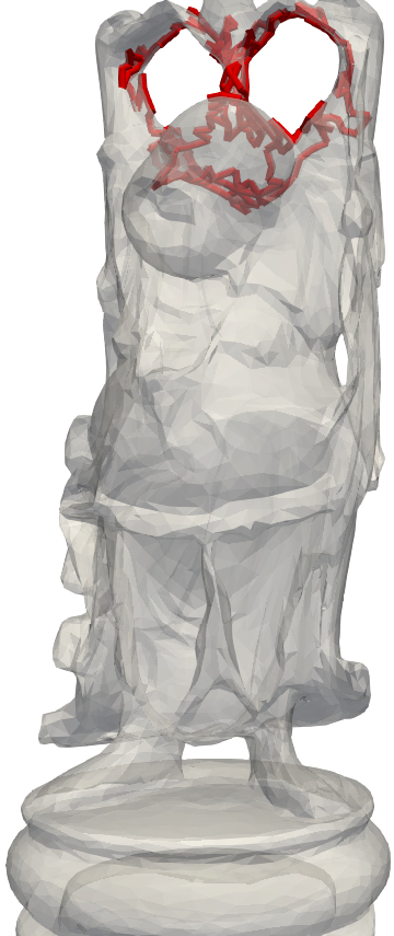
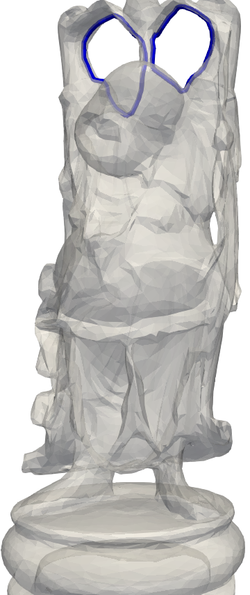
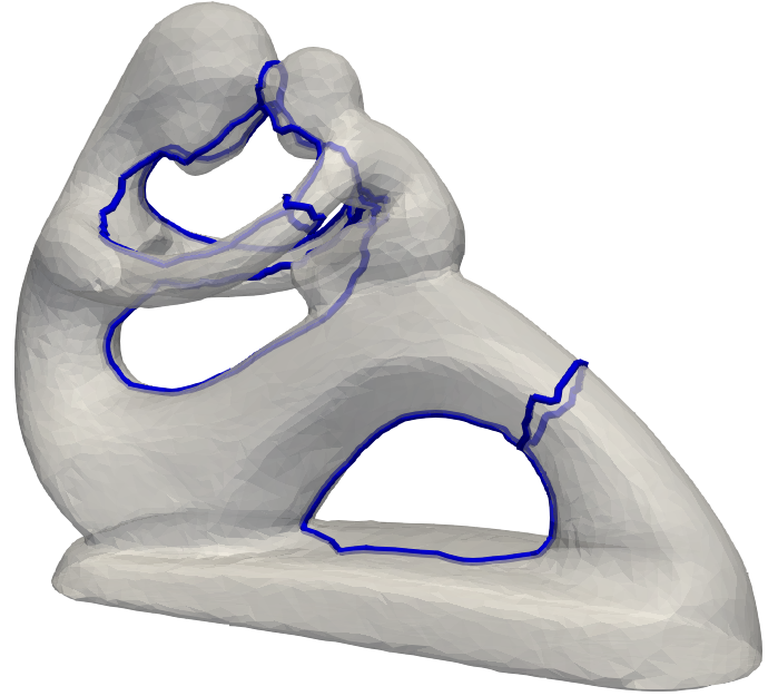
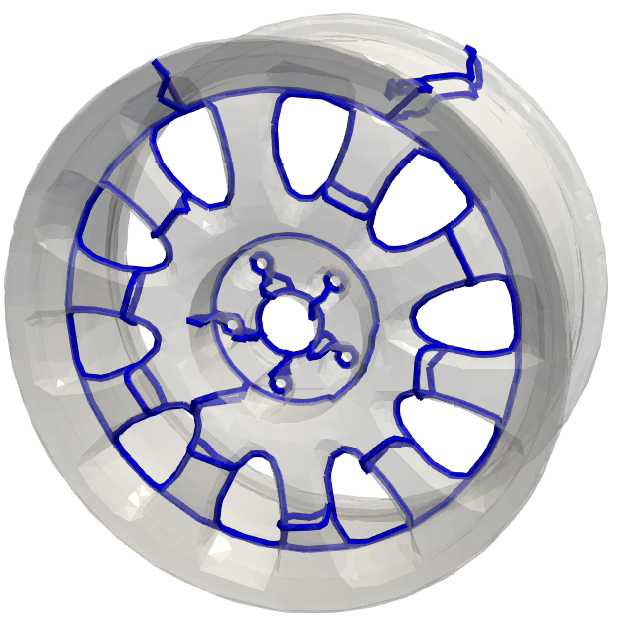
Figure 1: (top) The localization algorithm computes optimal (blue) 1-cycles that are homologous to input 1-cycles (red). (bottom) Minimum 1-homology basis.

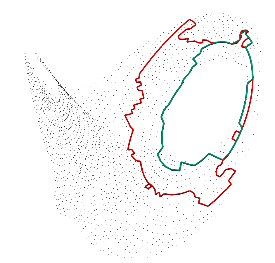
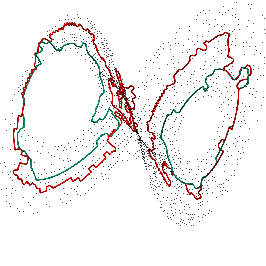
(a) Lorenz’63(60%)	(b) Lorenz’63(80%)
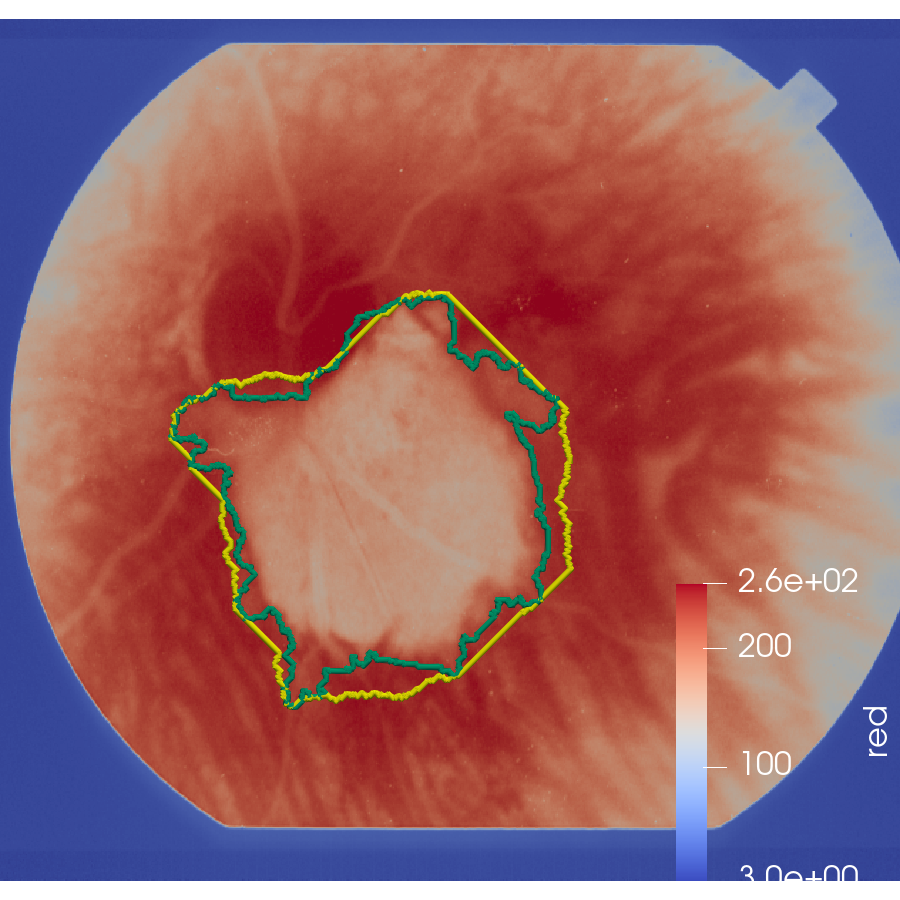
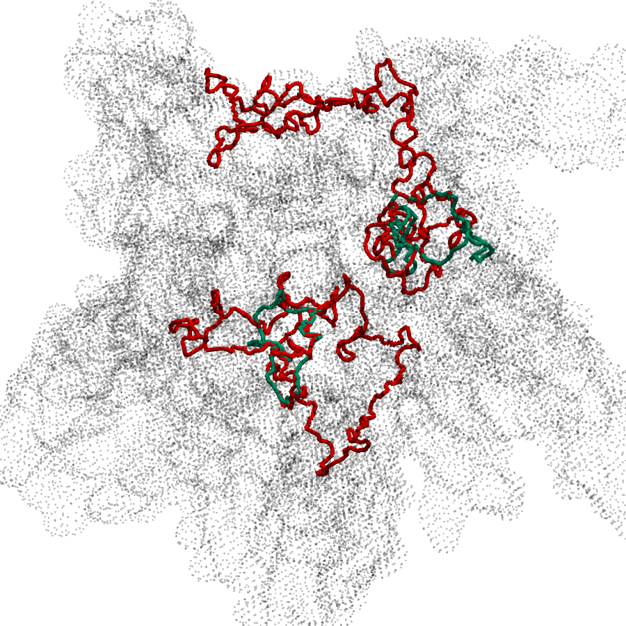
(c) Retina	(d) 1OED

Figure 2: The green persistent 1-homology cycles computed by our algorithm are tighter than the red (or yellow) cycles computed by PersLoop [15].

Homology localization.

Given an input simplicial complex representing a surface and a 1-cycle, we compute a localized cycle that is homologous to the input cycle. Figure 1(top) shows two input cycles (red) and their localized versions (blue) for the Happy Buddha dataset. We can visually infer that the localized cycle computed by our approximate algorithm is close to the optimal cycle.

Optimal homology basis.

Figure 1(bottom) shows the optimal homology basis computed for two 3D models. We observe that the cycles are tight and capture all tunnels and loops of the model. Results on additional datasets are available in Appendix D.

Optimal persistent homology cycle.

We report our results on three classes of filtrations: Rips, lower star, and Delaunay. Figure 2 (a,b) shows the Lorenz’63 data set for 60% and 80% densities and the representatives of the longest and the top two longest bars, respectively, of a Rips filtration. These are of relevance in simulating weather phenomena [29]. Figure 2 (c) highlights the representative of the longest lived bar for a lower star filtration on a retinal image [23] with a retinal disorder. The cycle represents the region of the disorder. Figure 2 (d) highlights representatives of the top two bars of an alpha complex on a protein molecule (PDB-ID: 1OED). Cycles computed by our algorithm (green) appear “tighter” than those computed by PersLoop (red or yellow).

Execution time.

Our algorithms are parallelizable if the optimization subroutines for each site can be executed independently. We obtain fast running times ($\sim$ few minutes) for moderate to large-sized datasets ($\sim$ millions of simplices) for all algorithms, see Table 1.

Data set	#Simplices	Execution time
Lorenz-63(60%)	$\sim 2\times 10^{6}$	120s
Lorenz-63(80%)	$\sim 3\times 10^{6}$	120s
Retina	$\sim 5\times 10^{6}$	140s
1OED	$\sim 2.5\times 10^{6}$	130s

Table 1: Mean time to compute optimal representative of each of the top-40 bars in the persistence barcode.

Appendix A Persistent homology

In this section, we provide the basic definitions for persistent homology, and the usual distances used in this context, namely, the interleaving distance and the matching distance.

Given a nested sequence of simplicial complexes indexed over $\mathbb{N}$, $\mathbb{Z}$, or $\mathbb{R}$, persistent homology of this sequence captures how a homology class evolves over the sequence. Formally, let $\mathcal{P}$ denote one of the poset categories $\mathbb{N}$, $\mathbb{Z}$, or $\mathbb{R}$. Given a finite complex $\mathsf{K}$, let $\mathcal{K}$ denote the set of all possible subcomplexes of $\mathsf{K}$ including the empty one. A $\mathcal{P}$-indexed filtration of $\mathsf{K}$ is a map $\mathcal{F}:\mathcal{P}\rightarrow\mathcal{K}$ that satisfies $\mathcal{F}(a)\subseteq\mathcal{F}(a^{\prime})$ for every pair of indices $a,a^{\prime}\in\mathcal{P}$ with $a\leq a^{\prime}$. In this case, $\mathcal{F}$ takes a sequence of real numbers

$$a_{0}\leq a_{1}\leq a_{2}\leq\dots$$

to a nested sequence of simplicial complexes $\mathsf{K}_{a_{i}}\subseteq\mathsf{K}$

$${\mathcal{F}}:\dots\hookrightarrow\mathsf{K}_{a_{0}}\hookrightarrow\mathsf{K}_{a_{1}}\hookrightarrow\mathsf{K}_{a_{2}}\hookrightarrow\dots$$

Using $p$-th homology groups of the complexes over the field $\mathbb{Z}_{2}$, we get a sequence of vector spaces connected by inclusion-induced linear maps:

$${H_{p}\mathcal{F}}:\dots\rightarrow H_{p}(\mathsf{K}_{a_{0}})\rightarrow H_{p}(\mathsf{K}_{a_{1}})\rightarrow H_{p}(\mathsf{K}_{a_{2}})\rightarrow\dots$$

For any pair $a_{i},a_{j}$, let $\iota_{i,j}:H_{p}(\mathsf{K}_{a_{i}})\rightarrow H_{p}(\mathsf{K}_{a_{j}})$ denote the linear map (internal morphism) induced by the inclusion $\mathsf{K}_{a_{i}}\hookrightarrow\mathsf{K}_{a_{j}}$. The sequence $H_{p}\mathcal{F}$ with the linear maps is called a persistence module which satisfies the following two properties : (i) for any triple $a_{i}\leq a_{j}\leq a_{k}$ in $\mathcal{P}$, one has $\iota_{i,k}=\iota_{j,k}\circ\iota_{i,j}$ and (ii) $\iota_{i,i}$ is identity for each $a_{i}\in\mathcal{P}$.

Let $b,d\in\mathcal{P}$. We define the interval $[b,d)$ as

$$[b,d)=\left\{a\in\mathcal{P}\mid b\leq a<d\right\}.$$

There is a special persistence module called the interval module ${\mathbb{I}}^{[b,d)}$ associated to the interval $[b,d)$. Denoting the vector space indexed at $a\in\mathcal{P}$ as ${\mathbb{I}}_{a}$, this interval module is given by

$${\mathbb{I}}_{a}^{[b,d)}=\begin{cases}\mathbb{Z}_{2}&\text{if $a\in[b,d)$}\\ 0&\text{otherwise}\end{cases}$$

together with identity maps $\operatorname{id}_{a,a^{\prime}}:{\mathbb{I}}_{a}^{[b,d)}\to{\mathbb{I}}_{a^{\prime}}^{[b,d)}$ for all $a,a^{\prime}\in[b,d)$ with $a\leq a^{\prime}$.

It is known due to a result of Gabriel [21] that a persistence module defined with finite complexes admits a decomposition

$$H_{p}{\mathcal{F}}\cong\bigoplus_{\alpha}{\mathbb{I}}^{[b_{\alpha},d_{\alpha})}$$ (4)

which is unique up to isomorphism and permutation of the intervals. The intervals $[b_{\alpha},d_{\alpha})$ are called the bars. The multiset of bars forms the barcode of the persistence module $H_{p}\mathcal{F}$. Let $B_{p}(\mathcal{F})$ denote this barcode for the filtration $\mathcal{F}$.

A.1 Interleavings and matchings for persistence modules

We need the following concept of interleavings between persistence modules in order to establish a stability property for the so called $\ell_{2}\text{--radius}$ for $\operatorname{\check{C}{ech}}$ filtrations. To make the discussion accessible to a computer science audience, we strip the presentation off its original category-theoretic formulation, and instead provide a more concrete and accessible description.

Definition ($\epsilon$-shifts of persistence modules).

Let $\epsilon$ be a non-negative real number, and let $\mathbb{P}$ be a persistence module with internal linear maps given by ${\phi}_{a,a^{\prime}}$. Then, the $\epsilon$-shift of $\mathbb{P}$, denoted by $\mathbb{P}^{\epsilon}$, is given by ${\mathbb{P}}_{a}^{\epsilon}={\mathbb{P}}_{a+\epsilon}$ with internal linear maps ${\phi}^{\epsilon}_{a,a^{\prime}}={\phi}_{a+\epsilon,a^{\prime}+\epsilon}$.

Definition ($\varepsilon$-interleaving).

Let $\mathbb{P}$ and $\mathbb{Q}$ be two persistence modules indexed over the real numbers and with the internal linear maps as ${\phi}_{a,a^{\prime}}$ and ${\psi}_{a,a^{\prime}}$ respectively. We say $\mathbb{P}$ and $\mathbb{Q}$ are $\varepsilon$-interleaved if there exist two families of maps $F_{a}:\mathbb{P}_{a}\rightarrow\mathbb{Q}_{a+\varepsilon}$ and $G_{a}:\mathbb{Q}_{a}\rightarrow\mathbb{P}_{a+\varepsilon}$ satisfying the following two conditions:

1. ${\psi}_{a+\varepsilon,a^{\prime}+\varepsilon}\circ F_{a}=F_{a^{\prime}}\circ{\phi}_{a,a^{\prime}}$ and ${\phi}_{a+\varepsilon,a^{\prime}+\varepsilon}\circ G_{a}=G_{a^{\prime}}\circ{\psi}_{a,a^{\prime}}$ [rectangular commutativity]

2. $G_{a+\varepsilon}\circ F_{a}={\phi}_{a,a+2\varepsilon}$ and $F_{a+\varepsilon}\circ G_{a}={\psi}_{a,a+2\varepsilon}$ [triangular commutativity]

Some of the relevant maps for interleaving between two modules are shown above whereas the two parallelograms and the two triangles below depict the rectangular and the triangular commutativities respectively.

Definition (Interleaving distance).

Given two persistence modules $\mathbb{P}$ and $\mathbb{Q}$, their interleaving distance is defined as

$$\mathrm{d}_{I}(\mathbb{P},\mathbb{Q})=\inf\{\varepsilon\,|\,\mbox{$\mathbb{P}$ and $\mathbb{Q}$ are $\varepsilon$-interleaved}\}.$$

Remark A.1.

In Section A.1, the family of maps $\{F_{a}\mid a\in\mathbb{R}\}$ assemble to give a map $F:\mathbb{P}\to\mathbb{Q}^{\epsilon}$, and the family of maps $\{G_{a}\mid a\in\mathbb{R}\}$ assemble to give a map $G:\mathbb{Q}\to\mathbb{P}^{\epsilon}$.

Definition ($\epsilon$-shift of a family of maps).

Suppose there exists a family of maps $F:\mathbb{P}\to\mathbb{Q}$. Then, a shift of $F$ by $\epsilon$, denoted by $F^{\epsilon}$, gives a new family maps $\{{F}^{\epsilon}_{a}={F}_{a+\epsilon}\mid a\in\mathbb{R}\}$ from $\mathbb{P}^{\epsilon}$ to $\mathbb{Q}^{\epsilon}$.

We now define the notion of $\epsilon$-matchings between two barcodes.

Definition ($\epsilon$-matching of barcodes).

Suppose that we are given two barcodes (which are multisets of intervals) $X$ and $Y$. Then, a matching $\mathcal{M}$ between $X$ and $Y$ is a collection of pairs $\mathcal{M}=\left\{(\mathbf{i},\mathbf{j})\mid\mathbf{i}\in X,\mathbf{j}\in Y\right\}$ such that each $\mathbf{i}$ and $\mathbf{j}$ occur in at most one pair.

Let $\mathcal{U}(\mathcal{M})$ be the collection of intervals in $X\cup Y$ that do not appear in any of the pairings of $\mathcal{M}$.

For pairs $(\mathbf{i},\mathbf{j})\in\mathcal{M}$ , where $\mathbf{i}=(b,d)$ and $\mathbf{j}=(b^{\prime},d^{\prime})$, define $c(\mathbf{i},\mathbf{j})=\max(|b-b^{\prime}|,|d-d^{\prime}|)$ and for intervals $\mathbf{i}=[b,d)\in\mathcal{U}$, define $c(\mathbf{i})=\frac{d-b}{2}$. Then, the cost of the matching $\mathcal{M}$, denoted by $c(\mathcal{M})$, is defined as follows:

$$c(\mathcal{M})=\max\left(\sup_{(\mathbf{i},\mathbf{j})\in\mathcal{M}}c((\mathbf{i},\mathbf{j})),\sup_{\mathbf{i}\in\mathcal{U}(\mathcal{M})}c(\mathbf{i})\right).$$

Finally, we say that $\mathcal{M}$ is an $\epsilon$-matching if $c(\mathcal{M})\leq\epsilon$.

Appendix B Approximate stability for $\ell_{2}$-radius

We now study notions of stability for weight functions that serve as objective functions for intervals in a barcode. We limit the discussion to $\operatorname{\check{C}{ech}}$ filtrations, while noting that similar definitions can be derived for other commonly encountered filtrations like Rips or lower star.

B.1 Stability of weight functions on intervals

We recall the notion of $\operatorname{\check{C}{ech}}$ complexes before proceeding to introduce some new definitions of our own concerning stability of weight functions on intervals.

Definition ($\operatorname{\check{C}{ech}}$ complexes).

Let $P$ be a finite point set in $\mathbb{R}^{d}$. Let $D_{r,x}$ denote a Euclidean ball of radius $r$ centered at $x$. The $\operatorname{\check{C}{ech}}$ complex of $P$ for radius $r$ is the abstract simplicial complex given by

$$\operatorname{\check{\mathsf{C}}}_{r}(P)=\{X\subset P\mid\bigcap_{x\in X}D_{r,x}\neq\emptyset\}.$$

The $\operatorname{\check{C}{ech}}$ filtration of $P$, denoted by $\operatorname{\check{\mathsf{C}}}(P)$, is the nested sequence of complexes $\{\operatorname{\check{\mathsf{C}}}_{r}(P)\}_{r\geq 0}$, where $\operatorname{\check{\mathsf{C}}}_{s}(P)\subseteq\operatorname{\check{\mathsf{C}}}_{t}(P)$ for $s\leq t$. We use the notation $B(\operatorname{\check{\mathsf{C}}}(P))$ to denote the barcode of $\operatorname{\check{\mathsf{C}}}(P)$.

Definition ($\epsilon$-perturbations of point sets).

We say that $Q$ is an $\epsilon$-perturbation of $P$ realized through a bijective map $f$, if $f$ maps points in $P$ to points in $Q$ such that $\|p-f(p)\|_{2}\leq\epsilon$.

Definition (Weight functions on persistent homology bases).

Given a filtration $\mathcal{F}$, and a $p$-th persistent homology basis $\Omega_{p}(\mathcal{F})$ of $\mathcal{F}$, a function that assigns a positive real number to every cycle in $\Omega_{p}(\mathcal{F})$ is called a weight function on the $p$-th persistent homology basis $\Omega_{p}(\mathcal{F})$ of $\mathcal{F}$. In this case, the (total) weight on $\Omega_{p}(\mathcal{F})$ is simply the sum of weights of basis cycles.

Definition (Weight functions on persistent barcodes).

For a filtration $\mathcal{F}$, its $p$-th barcode $B_{p}(\mathcal{F})$, a persistent $p$-homology basis $\Omega_{p}(\mathcal{F})=\{\zeta_{1}\dots\zeta_{|\Omega_{p}(\mathcal{F})|}\}$, and a weight function $s$ on $\Omega_{p}(\mathcal{F})$ defined as $s(\Omega^{p}(\mathcal{F}))=\sum_{i=1}^{|\Omega_{p}(\mathcal{F})|}s(\zeta_{i})$, a weight function $w$ on $B_{p}(\mathcal{F})$ is defined as:

$$w(B_{p}(\mathcal{F}))=\min_{\Omega_{p}(\mathcal{F})}\,\,s(\Omega_{p}(\mathcal{F}))\quad\text{ where }\Omega_{p}(\mathcal{F})\text{ is a persistent $p$-homology basis for $\mathcal{F}$.}$$ (5)

If $\Omega^{\star}_{p}(\mathcal{F})$ is a persistent $p$-homology basis of minimum weight in Equation 5, then the weight $w([b,d))$ for an interval $[b,d)\in B_{p}(\mathcal{F})$ is defined as $w([b,d))=s(\zeta^{\star})$ where $\zeta^{\star}$ is the representative for $[b,d)$ in $\Omega^{\star}_{p}(\mathcal{F})$.

Definition (Stability of weight functions for filtration families).

Suppose that we are given a weight function $w$ on barcodes of a family of filtrations. Then, for a point set $P$, an associated filtration of complexes $\mathcal{F}_{P}$ and for real numbers $\epsilon,\delta\geq 0$, we say $w$ is $(\epsilon,\delta)$-stable for an interval $[b,d)\in B(\mathcal{F}_{P})$ with $(d-b)>2\epsilon$, if for every $\epsilon$-perturbation $Q$ of $P$ with an associated filtration of complexes $\mathcal{F}_{Q}$, there exists an $\epsilon$-matching $\mathcal{M}$ between the intervals of $B(\mathcal{F}_{P})$ and the intervals of $B(\mathcal{F}_{Q})$ such that if the length of the interval $\mathcal{M}([b,d))>2\epsilon$ then

$$|w([b,d))-w(\mathcal{M}([b,d)))|\leq 2\delta.$$

Furthermore, if $w$ is $(\epsilon,\delta)$-stable for all intervals of $B(\mathcal{F}_{P})$, then we say that $w$ is $(\epsilon,\delta)$-stable for the point set $P$. Finally, if $w$ is $(\epsilon,\delta)$-stable for every point set embedded in a Euclidean space, then we say that $w$ is $(\epsilon,\delta)$-stable for the filtration family.

Definition (Instability of weight functions).

Given a family of filtrations $\mathfrak{F}$, and a weight function $w$ defined on the persistent barcodes of filtrations belonging to $\mathfrak{F}$, we say that the pair $(\mathfrak{F},w)$ is unstable, if for every $\epsilon,\alpha>0$, there exists filtrations $\mathcal{F}_{1},\mathcal{F}_{2}\in\mathfrak{F}$ such that the barcodes of $\mathcal{F}_{1},\mathcal{F}_{2}\in\mathfrak{F}$ admit an $\epsilon$-matching while satisfying $|w(\mathcal{F}_{1})-w(\mathcal{F}_{2})|>\alpha$.

Figure 3: Two $1$-cycles $\xi_{1}$ and $\xi_{2}$ appear at time (index) $1$ and $2$ respectively. In the upper filtration, the green triangles appear at time $3$ filling up the annulus and the golden triangle appears at time $4$ giving rise to the bars $[2,3)$ and $[1,4)$ with the minimal (lengthwise) persistent cycles $\xi_{1}+\xi_{2}$ and $\xi_{1}$ resp. In the lower filtration the golden triangle comes first and green triangles next giving rise to slightly perturbed bars $[1,3)$ and $[2,4)$. Their minimal persistent cycles change to $\xi_{1}$ and $\xi_{2}$, resp. suggesting that the cycles may change considerably with respect to the length function.

In Figure 3, we provide an example depicting instability for the weight function given by length of $1$-cycles. While this is not the same as the $\ell_{2}\text{--radius}$, we maintain that similar counterexamples can be designed for $\ell_{2}\text{--radius}$ as well. We leave out the details here. In particular, it is easily seen that $\ell_{2}\text{--radius}$ is an unstable function for $\operatorname{\check{C}{ech}}$ filtrations.

B.2 Approximate representatives and bases

Given the inherent instability associated to the $\ell_{2}\text{--radius}$, we formulate a slightly weaker notion of stability for the $\ell_{2}\text{--radius}$. To state the result, we need a few definitions.

Definition ($\epsilon$-approximate representatives).

For an interval $[b,d)$ with $(d-b)>2\epsilon$, a cycle $\zeta$ is said to be an $\epsilon$-approximate representative for $[b,d)$, if $\zeta$ is a nontrivial cycle that is born at $b^{\prime}\in[b-\epsilon,b+\epsilon]$ and dies at $d^{\prime}\in[d-\epsilon,d+\epsilon]$, and the class $[\zeta]$ is nontrivial in $\mathsf{K}_{s}$ for every $s\in[b^{\prime},d^{\prime})$.

Recall that in Section 4, we provided a definition for the $\ell_{2}\text{--radius}$ function $r$ for intervals defined on chains and cycles of all subcomplexes of a complex $\mathsf{K}$, whose vertex set is embedded in a Euclidean space. We now provide a definition for an approximate variant of this function.

Definition ($\epsilon$-approximate radii of intervals).

As an approximation of the radius function defined in Equation 3, we now define $r^{\epsilon}([b,d))$ for an interval $[b,d)\in B(\operatorname{\check{\mathsf{C}}}(P))$ with $d-b>2\epsilon$ to be the radius of the smallest Euclidean sphere that encloses all the vertices of some $\epsilon$-approximate representative cycle of $[b,d)$. In other words, $r^{\epsilon}([b,d))=\min_{\zeta}r(\zeta)$, where $\zeta$ is an $\epsilon$-approximate representative cycle for $[b,d)$.

In Appendix B, we prove the following stability theorem (2 restated as 4 with a proof) by building on techniques developed by Bjerkevik [1].

Theorem 2 (Approximate stability for $\ell_{2}\text{--radius}$).

Let $P$ be a point set embedded in a Euclidean space and $Q$ be an $\epsilon$-perturbation of $P$. Then, there exists an $\epsilon$-matching $\mathcal{M}$ between $B(\operatorname{\check{\mathsf{C}}}(P))$ and $B(\operatorname{\check{\mathsf{C}}}(Q))$ such that if $[b^{\prime},d^{\prime})=\mathcal{M}([b,d))$ and both $[b,d)$, $[b^{\prime},d^{\prime})$ have lengths greater than $2\epsilon$, then

$$r^{2\epsilon}([b,d)) \leq r([b^{\prime},d^{\prime}))+\epsilon,$$

$$r^{2\epsilon}([b^{\prime},d^{\prime})) \leq r([b,d))+\epsilon.$$ (6)

Note that, as per Section B.1, we would have $(\epsilon,\epsilon)$ stability for $\ell_{2}\text{--radius}$, if there exists an $\epsilon$-matching $\mathcal{M}$ that matches intervals $[b,d)\in B(\operatorname{\check{\mathsf{C}}}(P))$ of length greater than $2\epsilon$ to intervals $[b^{\prime},d^{\prime})\in B(\operatorname{\check{\mathsf{C}}}(Q))$ of length greater than $2\epsilon$ satisfying

$$r([b,d)) \leq r([b^{\prime},d^{\prime}))+\epsilon,$$

$$r([b^{\prime},d^{\prime})) \leq r([b,d))+\epsilon.$$ (7)

In this sense, 2 is an approximate version of $\ell_{2}\text{--radius}$ stability.

We now build towards a proof for 2. To begin with, let $P$ be a point set embedded in a Euclidean space, and let $Q$ be an $\epsilon$-perturbation of $P$ realized through a bijective map between point sets denoted by $f$. We denote the inverse of $f$ by $g$. Let ${\Omega}^{P}=\{\zeta_{1},\zeta_{2},\dots,\zeta_{n}\}$ be a persistent homology basis for $\operatorname{\check{\mathsf{C}}}(P)$, and let ${\Omega}^{Q}=\{z_{1},z_{2},\dots,z_{m}\}$ be a persistent homology basis for $\operatorname{\check{\mathsf{C}}}(Q)$.

Then, it is easy to check that for every $s\in\mathbb{R}$, the map $f$ induces a simplicial map $f_{s}:\operatorname{\check{\mathsf{C}}}_{s}(P)\to\operatorname{\check{\mathsf{C}}}_{s+\epsilon}(Q)$. Furthermore, the map $f_{s}$ induces a map on the respective cycle groups ${f}_{s}^{\#}:Z_{\ast}(\operatorname{\check{\mathsf{C}}}_{s}(P))\to Z_{\ast}(\operatorname{\check{\mathsf{C}}}_{s+\epsilon}(Q))$ as well as a map $\hat{f}_{s}:H_{\ast}(\operatorname{\check{\mathsf{C}}}_{s}(P))\to H_{\ast}(\operatorname{\check{\mathsf{C}}}_{s+\epsilon}(Q))$ on homology groups.

Similarly, for every $s\in\mathbb{R}$, the map $g$ induces a simplicial map $g_{s}:\operatorname{\check{\mathsf{C}}}_{s}(Q)\to\operatorname{\check{\mathsf{C}}}_{s+\epsilon}(P)$, which in turn, induces a map on the respective cycle groups ${g}_{s}^{\#}:Z_{\ast}(\operatorname{\check{\mathsf{C}}}_{s}(Q))\to Z_{\ast}(\operatorname{\check{\mathsf{C}}}_{s+\epsilon}(P))$ as well as a map on homology groups $\hat{g}_{s}:H_{\ast}(\operatorname{\check{\mathsf{C}}}_{s}(Q))\to H_{\ast}(\operatorname{\check{\mathsf{C}}}_{s+\epsilon}(P))$. Moreover, $g_{s+\epsilon}\circ f_{s}=\operatorname{id}$, and $f_{s+\epsilon}\circ g_{s}=\operatorname{id}$ for every $s\in\mathbb{R}$.

We define persistent modules $\mathbb{P}$ and $\mathbb{Q}$ as follows.

$$\mathbb{P}\quad =\quad\bigoplus_{\begin{subarray}{c}\mathbf{i}\in B(\operatorname{\check{\mathsf{C}}}(P))\\ \zeta_{i}\in\mathcal{R}(\mathbf{i})\end{subarray}}{\mathbb{I}}^{\zeta_{i}} \cong\quad\bigoplus_{\mathbf{i}\in B(\operatorname{\check{\mathsf{C}}}(P))}\mathbb{I}^{\mathbf{i}},$$

$$\mathbb{Q}\quad =\quad\bigoplus_{\begin{subarray}{c}\mathbf{j}\in B(\operatorname{\check{\mathsf{C}}}(Q))\\ z_{j}\in\mathcal{R}(\mathbf{j})\end{subarray}}{\mathbb{I}}^{z_{j}} \cong\quad\bigoplus_{\mathbf{j}\in B(\operatorname{\check{\mathsf{C}}}(Q))}\mathbb{I}^{\mathbf{j}}.$$

For some $\mathbf{j}=[b_{j},d_{j})\in B(\operatorname{\check{\mathsf{C}}}(Q))$, let $z_{j}\in\mathcal{R}(\mathbf{j})$. Then, $\hat{g}_{\vphantom{1^{H}}b_{j}}([z_{j}])$ is a class in $\operatorname{\check{\mathsf{C}}}_{b_{j}+\epsilon}(P)$. Since ${\Omega}^{P}$ is a persistent homology basis for $\operatorname{\check{\mathsf{C}}}(P)$, $\hat{g}_{\vphantom{1^{H}}b_{j}}([z_{j}])$ can be written as follows.

$$\hat{g}_{\vphantom{1^{H}}b_{j}}([z_{j}])=\sum_{i\in I}\kappa_{j,i}\cdot[\zeta_{i}].$$ (8)

In Equation 8, $I\subset[n]$ indexes a subset of the representative cycles for the intervals in $B(\operatorname{\check{\mathsf{C}}}(P))$, and the coefficients $\kappa_{j,i}\in\mathbb{Z}_{2}$.

We define $G|_{\mathbf{j}}:{\mathbb{I}}^{z_{j}}\to\mathbb{P}^{\epsilon}$ as follows.

$$G|_{\mathbf{j}}({\mathbb{I}}^{z_{j}}_{s})=\sum_{i\in I}\kappa_{j,i}\cdot{{\mathbb{I}}^{\zeta_{i}}_{s+\epsilon}}\quad\text{ for $s\in[b_{j},d_{j})$}.$$

By linear extension over all intervals $\mathbf{j}\in B(\operatorname{\check{\mathsf{C}}}(Q))$, we obtain a map $G:\mathbb{Q}\to\mathbb{P}^{\epsilon}$.

Symmetrically, let $\zeta_{i}\in{\Omega}^{P}$ be a representative cycle for some $\mathbf{i}=[b_{i},d_{i})\in B(\operatorname{\check{\mathsf{C}}}(P))$. Then, $\hat{f}_{\vphantom{1^{H}}b_{i}}([\zeta_{i}])$ is a class in $\operatorname{\check{\mathsf{C}}}_{b_{i}+\epsilon}(Q)$ Thus, $\hat{f}_{\vphantom{1^{H}}b_{i}}([\zeta_{i}])$ can be written as follows.

$$\hat{f}_{\vphantom{1^{H}}b_{i}}([\zeta_{i}])=\sum_{j\in J}\eta_{i,j}\cdot[z_{j}].$$ (9)

In Equation 9, $J\subset[m]$ indexes a subset of the representative cycles for intervals in $B(\operatorname{\check{\mathsf{C}}}(Q))$, and the coefficients $\eta_{i,j}\in\mathbb{Z}_{2}$.

We define $F|_{\mathbf{i}}:{\mathbb{I}}^{\zeta_{i}}\to\mathbb{Q}^{\epsilon}$ as follows.

$$F|_{\mathbf{i}}({\mathbb{I}}^{\zeta_{i}}_{s})=\sum_{j\in J}\eta_{i,j}\cdot{{\mathbb{I}}^{z_{j}}_{s+\epsilon}}\quad\text{ for $s\in[b_{i},d_{i})$}.$$

By linear extension over all intervals $\mathbf{i}\in B(\operatorname{\check{\mathsf{C}}}(P))$, we obtain a map $F:\mathbb{P}\to\mathbb{Q}^{\epsilon}$.

It is easy to check that the maps $F$ and $G$ consitute an $\epsilon$-interleaving between modules $\mathbb{P}$ and $\mathbb{Q}$. This is a simple consequence of the fact that $g_{s+\epsilon}\circ f_{s}=\operatorname{id}$, and $f_{s+\epsilon}\circ g_{s}=\operatorname{id}$ for every $s\in\mathbb{R}$.

Let $\imath^{\mathbb{P}}_{\mathbf{i}}:{\mathbb{I}}^{\zeta_{i}}\xhookrightarrow{}\mathbb{P}$ and $\imath^{\mathbb{Q}}_{\mathbf{j}}:{\mathbb{I}}^{z_{j}}\xhookrightarrow{}\mathbb{Q}$ denote the canonical inclusion maps, and let $\pi^{\mathbb{P}}_{\mathbf{i}}:\mathbb{P}\twoheadrightarrow{\mathbb{I}}^{\zeta_{i}}$ and $\pi^{\mathbb{Q}}_{\mathbf{j}}:\mathbb{Q}\twoheadrightarrow{\mathbb{I}}^{z_{j}}$ denote the canonical projection maps.

For the morphism $F:\mathbb{P}\to\mathbb{Q}^{\epsilon}$, we have $F|_{\mathbf{i}}=F\circ\imath^{\mathbb{P}}_{\mathbf{i}}$. Now, let $F_{\mathbf{i},\mathbf{j}}={(\pi^{\mathbb{Q}}_{\mathbf{j}})}^{\epsilon}\circ F\circ\imath^{\mathbb{P}}_{\mathbf{i}}$. Likewise, for the morphism $G:\mathbb{Q}\to\mathbb{P}^{\epsilon}$, we have $G|_{\mathbf{j}}=G\circ\imath^{\mathbb{Q}}_{\mathbf{j}}$. Now, let $G_{\mathbf{j},\mathbf{i}}={(\pi^{\mathbb{P}}_{\mathbf{i}})}^{\epsilon}\circ G\circ\imath^{\mathbb{Q}}_{\mathbf{j}}$.

Let $\phi^{\epsilon}:\mathbb{P}\to\mathbb{P}^{\epsilon}$ denote the collection of maps whose restriction to $\mathbb{P}_{t}$ gives the internal linear map $\phi_{t,t+\epsilon}:\mathbb{P}_{t}\to\mathbb{P}_{t+\epsilon}$. For an interval summand ${\mathbb{I}}^{\mathbf{i}}$ of $\mathbb{P}$, let $\phi_{\mathbf{i}}^{\epsilon}$ denote the collection of maps whose restriction to ${\mathbb{I}}^{\mathbf{i}}_{t}$ gives the internal linear map $\phi_{t,t+\epsilon}|_{{\mathbb{I}}^{\mathbf{i}}}:{\mathbb{I}}_{t}\to{\mathbb{I}}_{t+\epsilon}$.

Using the fact that $\phi_{\mathbf{i}}^{2\epsilon}={(\pi^{\mathbb{P}}_{\mathbf{i}})}^{2\epsilon}\circ\phi^{2\epsilon}\circ\imath^{\mathbb{P}}_{\mathbf{i}}$, we can write

$$\phi_{\mathbf{i}}^{2\epsilon}\quad=\quad\sum_{\mathbf{j}\in B(\operatorname{\check{\mathsf{C}}}(Q))}G_{\mathbf{j},\mathbf{i}}^{\epsilon}\circ F_{\mathbf{i},\mathbf{j}}.$$ (10)

Moreover, because $\mathbb{P}$ is a direct sum of interval modules, for $\mathbf{i}\neq\mathbf{i}^{\prime}$, we obtain

$${(\pi^{\mathbb{P}}_{\mathbf{i}^{\prime}})}^{2\epsilon}\circ\phi^{2\epsilon}\circ\imath^{\mathbb{P}}_{\mathbf{i}}\quad =\quad\sum_{\mathbf{j}\in B(\operatorname{\check{\mathsf{C}}}(Q))}G_{\mathbf{j},\mathbf{i}^{\prime}}^{\epsilon}\circ F_{\mathbf{i},\mathbf{j}}$$

$$=\quad 0.$$ (11)

Definition ($\Lambda(\mathbf{i}),\Lambda(A)$).

For intervals $\mathbf{i}\in B(\operatorname{\check{\mathsf{C}}}(P))$, we define

$$\widetilde{\Lambda}(\mathbf{i}) =\{\mathbf{j}\in B(\operatorname{\check{\mathsf{C}}}(Q)):{\mathbb{I}}^{\mathbf{i}}\text{ and }{\mathbb{I}}^{\mathbf{j}}\text{ are }\epsilon\text{-interleaved}\}\text{, and}$$

$$\Lambda(\mathbf{i}) =\{\mathbf{j}\in B(\operatorname{\check{\mathsf{C}}}(Q)):{\mathbb{I}}^{\mathbf{i}}\text{ and }{\mathbb{I}}^{\mathbf{j}}\text{ are }\epsilon\text{-interleaved and either }\eta_{i,j}\neq 0\text{ or }\kappa_{j,i}\neq 0\}.$$

For a collection of intervals $A\subset B(\operatorname{\check{\mathsf{C}}}(P))$, we define

$$\widetilde{\Lambda}(A)=\bigcup_{\mathbf{i}\in A}\widetilde{\Lambda}(\mathbf{i})\quad\text{ and }\quad\Lambda(A)=\bigcup_{\mathbf{i}\in A}\Lambda(\mathbf{i}).$$

Definition ($\Upsilon(\mathbf{j}),\Upsilon(A)$).

For intervals $\mathbf{j}\in B(\operatorname{\check{\mathsf{C}}}(Q))$, we define

$$\widetilde{\Upsilon}(\mathbf{j}) =\{\mathbf{i}\in B(\operatorname{\check{\mathsf{C}}}(P)):{\mathbb{I}}^{\mathbf{i}}\text{ and }{\mathbb{I}}^{\mathbf{j}}\text{ are }\epsilon\text{-interleaved}\}\text{, and}$$

$$\Upsilon(\mathbf{j}) =\{\mathbf{i}\in B(\operatorname{\check{\mathsf{C}}}(P)):{\mathbb{I}}^{\mathbf{i}}\text{ and }{\mathbb{I}}^{\mathbf{j}}\text{ are }\epsilon\text{-interleaved and either }\eta_{i,j}\neq 0\text{ or }\kappa_{j,i}\neq 0\}.$$

For a collection of intervals $A\subset B(\operatorname{\check{\mathsf{C}}}(Q))$, we define

$$\widetilde{\Upsilon}(A)=\bigcup_{\mathbf{j}\in A}\widetilde{\Upsilon}(\mathbf{j})\quad\text{ and }\quad\Upsilon(A)=\bigcup_{\mathbf{j}\in A}\Upsilon(\mathbf{j}).$$

Remark B.1.

From Sections B.2 and B.2 we make the following observations.

$$\mathbf{j}\in\widetilde{\Lambda}(A)\setminus\Lambda(A)\quad\Longrightarrow\quad\eta_{i,j}=0\text{ and }\kappa_{j,i}=0\text{ for all }\mathbf{i}\in A.$$

$$\mathbf{i}\in\widetilde{\Upsilon}(A)\setminus\Upsilon(A)\quad\Longrightarrow\quad\eta_{i,j}=0\text{ and }\kappa_{j,i}=0\text{ for all }\mathbf{j}\in A.$$

Remark B.2.

The sets $\widetilde{\Lambda}(A)$ is equivalent to $\mu(A)$ as defined in Botnan’s lecture notes [6][Section 13.2]. The rationale behind defining $\Lambda(A)$ and $\Upsilon(A)$ is to ensure that the representative cycles of perturbed sets can be linearly related. Refer to Remark B.5,4 for additional details.

We now recall some elementary propositions from Botnan’s lecture notes[6]. The proofs for Sections B.2, B.2 and B.2 can be found in Section 13.2 of [6].

Proposition .

For a morphism $\varrho:\mathbb{I}^{[b_{1},d_{1})}\to\mathbb{I}^{[b_{2},d_{2})}$, if $b_{2}>b_{1}$ or $d_{2}>d_{1}$, then $\varrho$ is zero. On the other hand, if $b_{2}\leq b_{1}$ and $d_{2}\leq d_{1}$, then $\varrho_{t}$ is determined by $\varrho_{b_{1}}$ for $t\in[b_{1},d_{2})$, in the sense that, $\varrho_{t}$ is nonzero if and only if $\varrho_{b_{1}}$ is nonzero.

Section B.2 above says that the morphism $\varrho:\mathbb{I}^{[b_{1},d_{1})}\to\mathbb{I}^{[b_{2},d_{2})}$ between interval modules is completely determined by the function value at $b_{1}$.

For an interval $\mathbf{i}=[b,d)$, define $\alpha(\mathbf{i})=b+d$. Specializing Bjerkevik’s arguments [1] to single parameter persistence, Botnan [6] defines the following preorder on single parameter interval modules: $\mathbf{i}\leq_{\alpha}\mathbf{j}$ if and only if $\alpha_{(}\mathbf{i})\leq\alpha_{(}\mathbf{j})$.

Proposition .

Let $\mathbf{i}_{1}={[b_{1},d_{1})}$, $\mathbf{i}_{2}={[b_{2},d_{2})}$ and $\mathbf{i}_{3}={[b_{3},d_{3})}$ be intervals such that $\mathbf{i}_{1}\leq_{\alpha}\mathbf{i}_{3}$. If there exist nonzero maps $\varrho:\mathbb{I}^{\mathbf{i}_{1}}\to{(\mathbb{I}^{\mathbf{i}_{2}})}^{\epsilon}$ and $\chi:\mathbb{I}^{\mathbf{i}_{2}}\to{(\mathbb{I}^{\mathbf{i}_{3}})}^{\epsilon}$, then $\mathbb{I}^{\mathbf{i}_{2}}$ is $\epsilon$-interleaved with either $\mathbb{I}^{\mathbf{i}_{1}}$ or $\mathbb{I}^{\mathbf{i}_{3}}$.

Remark B.3.

When $\mathbf{i}_{3}=\mathbf{i}_{1}$, the contrapositive of Section B.2 reads as follows: If $\mathbb{I}^{\mathbf{i}_{2}}$ is not $\epsilon$-interleaved with $\mathbb{I}^{\mathbf{i}_{1}}$, then either $\varrho:\mathbb{I}^{\mathbf{i}_{1}}\to{(\mathbb{I}^{\mathbf{i}_{2}})}^{\epsilon}$ or $\chi:\mathbb{I}^{\mathbf{i}_{2}}\to{(\mathbb{I}^{\mathbf{i}_{3}})}^{\epsilon}$ is a zero map.

Proposition .

Let $\mathbf{i}_{1}=[b_{1},d_{1})$, $\mathbf{i}_{2}=[b_{2},d_{2})$ and $\mathbf{i}_{3}=[b_{3},d_{3})$ be such that $(d_{1}-b_{1})>2\epsilon$, $(d_{3}-b_{3})>2\epsilon$ and $\mathbf{i}_{1}\leq_{\alpha}\mathbf{i}_{3}$. If there exist nonzero maps $\varrho:\mathbb{I}^{\mathbf{i}_{1}}\to{(\mathbb{I}^{\mathbf{i}_{2}})}^{\epsilon}$ and $\chi:\mathbb{I}^{\mathbf{i}_{2}}\to{(\mathbb{I}^{\mathbf{i}_{3}})}^{\epsilon}$, then $\chi^{\epsilon}\circ\varrho\neq 0$.

Remark B.4.

It is worth noting that Section B.2 applies only when $\mathbf{i}_{1}{\leq}_{\alpha}\mathbf{i}_{3}$. When $\mathbf{i}_{1}>_{\alpha}\mathbf{i}_{3}$, there is no guarantee that $\chi^{\epsilon}\circ\varrho$ is nonzero even when $\varrho$ and $\chi$ are both nonzero. Later, in Section B.2, this has implications in how Equation 16 is set up.

Proposition .

Suppose $\mathbb{P}$ and $\mathbb{Q}$ are $\epsilon$-interleaved. Let $A$ be a collection of intervals in $\mathbb{P}$ with length greater than $2\epsilon$. Then, $|A|\leq|\Lambda(A)|$.

Proof.

Let $\mu=|A|$ and $\nu=|\Lambda(A)|$. To begin with, order the elements of $A=\{\mathbf{i}_{1},\mathbf{i}_{2},\dots,\mathbf{i}_{\mu}\}$ in non-decreasing order of $\leq_{\alpha}$. Also, for $\mathbf{i}=[b_{i},d_{i})$ and $\mathbf{i}^{\prime}=[b_{i^{\prime}},d_{i^{\prime}})$, we write $i<i^{\prime}$ if and only if $\mathbf{i}\leq_{\alpha}\mathbf{i}^{\prime}$. Let $\Lambda(A)=\{\mathbf{j}_{1},\mathbf{j}_{2},\dots,\mathbf{j}_{\nu}\}$.

Next, we obtain an expression for $\phi_{\mathbf{i}}^{2\epsilon}$ as follows.

$$\phi_{\mathbf{i}}^{2\epsilon}\quad =\quad\sum_{\mathbf{j}\in B(\operatorname{\check{\mathsf{C}}}(Q))}G_{\mathbf{j},\mathbf{i}}^{\epsilon}\circ F_{\mathbf{i},\mathbf{j}}\quad$$ using Equation 10

$$=\quad\sum_{\mathbf{j}\in\widetilde{\Lambda}(A)}G_{\mathbf{j},\mathbf{i}}^{\epsilon}\circ F_{\mathbf{i},\mathbf{j}}\quad$$ using Remark B.3

$$=\quad\sum_{\mathbf{j}\in\Lambda(A)}G_{\mathbf{j},\mathbf{i}}^{\epsilon}\circ F_{\mathbf{i},\mathbf{j}}$$ using Remark B.1. (12)

Using the same observation, for $\mathbf{i}\leq_{\alpha}\mathbf{i}^{\prime}$, we obtain the following expression:

$$\sum_{\mathbf{j}\in\Lambda(A)}G_{\mathbf{j},\mathbf{i}^{\prime}}^{\epsilon}\circ F_{\mathbf{i},\mathbf{j}}\quad =\quad\sum_{\mathbf{j}\in\widetilde{\Lambda}(A)}G_{\mathbf{j},\mathbf{i}^{\prime}}^{\epsilon}\circ F_{\mathbf{i},\mathbf{j}}$$ using Remark B.1

$$=\quad\sum_{\mathbf{j}\in B(\operatorname{\check{\mathsf{C}}}(Q))}G_{\mathbf{j},\mathbf{i}^{\prime}}^{\epsilon}\circ F_{\mathbf{i},\mathbf{j}}\quad$$ using Section B.2

$$=\quad 0\quad \text{ using \lx@cref{creftypecap~refnum}{eq:zeroex}}.$$ (13)

Using Sections B.2 and B.2, Proof and Proof can be written as

$$1\quad =\quad\sum_{\mathbf{j}\in\Lambda(\mathbf{i})}\kappa_{j,i}\cdot\eta_{i,j}\quad\text{and}$$ (14)

$$0\quad =\quad\sum_{\mathbf{j}\in\Lambda(\mathbf{i})}\kappa_{j,i^{\prime}}\cdot\eta_{i,j}\text{ for $i<i^{\prime}$, respectively.}$$ (15)

Putting Equations 14 and 15 in matrix form yields the following matrix equation, where the entries above the diagonal in the right hand side matrix are unknown.

$$\left[\begin{matrix}\kappa_{j_{1},i_{1}}&\dots&\kappa_{j_{\nu},i_{1}}\\ \vdots&\ddots&\vdots\\ \kappa_{j_{1},i_{\mu}}&\dots&\kappa_{j_{\nu},i_{\mu}}\end{matrix}\right]\left[\begin{matrix}\eta_{i_{1},j_{1}}&\dots&\eta_{i_{\mu},j_{1}}\\ \vdots&\ddots&\vdots\\ \eta_{i_{1},j_{\nu}}&\dots&\eta_{i_{\mu},j_{\nu}}\end{matrix}\right]=\left[\begin{matrix}1&\ast&\dots&\ast\\ 0&1&\dots&\ast\\ 0&0&\ddots&\vdots\\ 0&0&\dots&1\end{matrix}\right].$$ (16)

Since the matrix on the right hand side is upper triangular with ones on diagonal, it has rank $|A|$. On the other hand, the two matrices on the left have rank upper bounded by $\nu=|\Lambda(A)|$. It follows immediately that $|A|\leq|\Lambda(A)|$.

Proposition .

Suppose $\mathbb{P}$ and $\mathbb{Q}$ are $\epsilon$-interleaved. Let $A$ be a collection of intervals in $\mathbb{Q}$ with length greater than $2\epsilon$. Then, $|A|\leq|\Upsilon(A)|$.

Proof.

The statement of the theorem is symmetric to Section B.2. Hence, we omit the details of the proof.

Remark B.5.

Note that the proof of Section B.2 closely follows Botnan’s exposition of Bjerkevik’s ideas for constructing an $\epsilon$-matching given an $\epsilon$-interleaving between persistence modules using Hall’s theorem. However, there are three important differences.

• In our proof, it is vital to use the canonical $\epsilon$-interleavings that are induced by the simplicial maps $f_{s}$ and $g_{s}$ for $s\in\mathbb{R}$ as described in Appendix B. In Bjerkevik’s approach an arbitrary $\epsilon$-interleaving can be used to derive an $\epsilon$-matching. See Figure 4 for an example.

• While for Bjerkevik’s result it suffices to establish the inequality $|A|\leq|\widetilde{\Lambda}(A)|$, for our purposes it is necessary to establish the stricter inequality $|A|\leq|\Lambda(A)|$. In particular, we require that an interval $\mathbf{i}$ is matched only to one of the intervals in $\Lambda(\mathbf{i})$.

• While Bjerkevik uses arbitary interval decompositions of persistent modules, we are required to use the decompositions that come from fixed choices of persistence homology bases. This has the following consequence: even when the $\epsilon$-interleaving maps $F$ and $G$ are canonical, the maps $F_{\mathbf{i},\mathbf{j}}$ and $G_{\mathbf{j},\mathbf{i}}$ depend on how we choose to represent the interval summands of $\mathbb{P}$ and $\mathbb{Q}$. Since $F_{\mathbf{i},\mathbf{j}}$ and $G_{\mathbf{j},\mathbf{i}}$ determine $\Lambda(\mathbf{i})$ for every $\mathbf{i}$, the underlying bipartite graph to be matched is determined by the choice of representative cycles. This in turn has a bearing on what kind of $\epsilon$-interleaved interval summands of $\mathbb{P}$ and $\mathbb{Q}$ get matched.

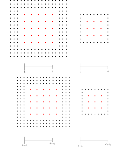
Figure 4: Consider the $\operatorname{\check{C}{ech}}$ filtrations on the point set shown in the top figure, denoted by $P$, which is $\delta$-perturbed to obtain another point set $Q$ shown in the bottom figure. In $\operatorname{\check{\mathsf{C}}}(P)$, the cycle on the left supported by the inner rim of black grid points, and the cycle on the right supported by black points are born at $b$ and die at $d$. Owing to a $\delta$-perturbation, where $\delta_{1},\delta_{2}<\delta$, in $\operatorname{\check{\mathsf{C}}}(Q)$, the first cycle is born at ${b+\delta_{1}}$ and dies at ${d+\delta_{1}}$, whereas the second cycle is born at ${b+\delta_{2}}$ and dies at ${d+\delta_{2}}$. If one uses Bjerkevik’s approach to obtain a $\delta$-matching, the bar $[b,d)$ (top left) may be matched to either the bar $[b+\delta_{1},d+\delta_{1})$ (bottom left) or $[b+\delta_{2},d+\delta_{2})$ (bottom right), whereas the bar $[b,d)$ (top right) may also be matched to either the bar $[b+\delta_{1},d+\delta_{1})$ (bottom left) or $[b+\delta_{2},d+\delta_{2})$ (bottom right). Thus, a naive approach to $\delta$-matching is not approximately stable as the radius values of the enclosing spheres of matched representatives can be arbitrarily far apart. Our version of matching ensures that for this example, $[b,d)$ (top left) is matched to $[b+\delta_{1},d+\delta_{1})$ (bottom left) and $[b,d)$ (top right) is matched to the bar $[b+\delta_{2},d+\delta_{2})$ (bottom right).

Theorem 3 (Hall’s theorem).

Let $G$ be a finite bipartite graph on sets $U$ and $V$. For a subset of vertices $U^{\prime}\subset U$, let $N_{G}(U^{\prime})$ denote the subset of $V$ adjacent to $U^{\prime}$. Then, the following are equivalent:

• for all $U^{\prime}\subset U$, $|U^{\prime}|\leq|N_{G}(U^{\prime})|$

• there exists an injective map $\imath:U\xhookrightarrow{}V$ such that $\imath$ maps every vertex $a$ of $U$ to a vertex $b$ of $V$ only if there is an edge $(a,b)$ in $G$.

Let ${\Omega}^{P}_{2\epsilon}\subseteq{\Omega}^{P}$ be the cycles of ${\Omega}^{P}$ that represent intervals of length greater than $2\epsilon$. Likewise, let ${\Omega}^{Q}_{2\epsilon}\subseteq{\Omega}^{Q}$ be the cycles of ${\Omega}^{Q}$ that represent intervals of length greater than $2\epsilon$. Since $\mathbb{P}$ and $\mathbb{Q}$ are $\epsilon$-interleaved, combining Section B.2 and 3, we obtain two injections $\imath:{\Omega}^{P}_{2\epsilon}\xhookrightarrow{}{\Omega}^{Q}$ and $\jmath:{\Omega}^{Q}_{2\epsilon}\xhookrightarrow{}{\Omega}^{P}$ such that

$$\imath({\zeta_{i}}) ={z_{j}}\quad\Longrightarrow\quad{\mathbb{I}}^{\zeta_{i}}\text{ and }{\mathbb{I}}^{z_{j}}\text{ are }\epsilon\text{-interleaved and either }F_{\mathbf{i},\mathbf{j}}\text{ or }G_{\mathbf{j},\mathbf{i}}\text{ is nonzero.}$$ (17)

$$\jmath({z_{j}}) ={\zeta_{i}}\quad\Longrightarrow\quad{\mathbb{I}}^{\zeta_{i}}\text{ and }{\mathbb{I}}^{z_{j}}\text{ are }\epsilon\text{-interleaved and either }F_{\mathbf{i},\mathbf{j}}\text{ or }G_{\mathbf{j},\mathbf{i}}\text{ is nonzero.}$$ (18)

Corollary .

There is a matching of representative cycles of $\operatorname{\check{\mathsf{C}}}(P)$ with representative cycles of $\operatorname{\check{\mathsf{C}}}(Q)$ such that

• All persistent cycles of $\operatorname{\check{\mathsf{C}}}(P)$ and $\operatorname{\check{\mathsf{C}}}(Q)$ representing intervals of length greater than $2\epsilon$ are matched.

• If a representative $\zeta_{i}$ of $\operatorname{\check{\mathsf{C}}}(P)$ is matched to a representative $z_{j}$ of $\operatorname{\check{\mathsf{C}}}(Q)$, then $\mathbb{I}^{\mathbf{i}}$ is $\epsilon$-interleaved with $\mathbb{I}^{\mathbf{j}}$, and either $F_{\mathbf{i},\mathbf{j}}$ or $G_{\mathbf{j},\mathbf{i}}$ is nonzero.

Proof.

The proof is essentially a paraphrase of the proof of Theorem 13.14 in Botnan’s notes [6].

Construct a bipartite graph $G=(V,E)$ with vertex set $V={\Omega}^{P}\bigcup{\Omega}^{Q}$. The vertices of ${\Omega}^{P}$ are colored red and the vertices of ${\Omega}^{Q}$ are colored blue. The edges of $G$ are built from the two injections $\imath:{\Omega}^{P}_{2\epsilon}\xhookrightarrow{}{\Omega}^{Q}$ and $\jmath:{\Omega}^{Q}_{2\epsilon}\xhookrightarrow{}{\Omega}^{P}$. In particular, we have a directed edge $\zeta\mathrel{\bullet\mkern-2.5mu{\rightarrow}}z$ if and only if $\imath(\zeta)=z$, and a directed edge $z\mathrel{\bullet\mkern-2.5mu{\rightarrow}}\zeta$ if and only if $\jmath(z)=\zeta$. It is easy to check that every connected component in $G$ is either a directed cycle or a directed path.

The matching $\mathcal{M}$ is constructed as follows. For every cycle, pick alternate edges and include them in $\mathcal{M}$. For every directed path, pick the odd numbered edges and include them in $\mathcal{M}$. As a consequence, all vertices incident on some directed cycle are matched. Also, all vertices on directed paths of odd length are matched. The only vertices that are not matched are the terminal vertices of paths with even length, and these terminal vertices are representative cycles for intervals of length smaller than $2\epsilon$. This shows that $\mathcal{M}$ is an $\epsilon$-matching.

Also, by construction of $\Lambda(A)$ and $\Upsilon(A)$ as described in Sections B.2 and B.2, we have a directed edge from interval $\mathbf{i}$ to $\mathbf{j}$ in $G$ only if they are $\epsilon$-interleaved and either $F_{\mathbf{i},\mathbf{j}}$ or $G_{\mathbf{j},\mathbf{i}}$ is nonzero, which proves the second claim.

Proposition .

For an interval $[b^{\prime},d^{\prime})\in B(\operatorname{\check{\mathsf{C}}}(Q))$ represented by $z_{j}$, let $\hat{g}_{\vphantom{1^{H}}b_{j}}([z_{j}])=\sum_{i\in I}\kappa_{j,i}\cdot[\zeta_{i}]$, where $I$ indexes a subset of representative cycles of $\operatorname{\check{\mathsf{C}}}(P)$. Let $\Omega=\{\zeta_{i}\mid i\in I\}$. Then, every cycle in the set $\Omega$ dies at or before $d^{\prime}+\epsilon$.

Proof.

Targeting a contradiction, suppose that there exists a partition of cycles $\Omega=\Omega_{1}\sqcup\Omega_{2}$, where the cycles in $\Omega_{1}$ die at or before $d^{\prime}+\epsilon$, whereas the cycles in $\Omega_{2}$ die after $d^{\prime}+\epsilon$. Then, Eqn.  8 can be written as

$$\sum_{\omega\in\Omega_{2}}[\omega]\,=\,\sum_{\gamma\in\Omega_{1}}[\gamma]\,+\,\hat{g}_{\vphantom{1^{H}}b_{j}}([z_{j}]).\,$$ (19)

First, note that $\hat{g}_{\vphantom{1^{H}}b_{j}}([z_{j}])$ is trivial at $d^{\prime}+\epsilon$ because $g$ is an $\epsilon$-perturbation and $z_{j}$ dies at $d^{\prime}$. Then, at $d^{\prime}+\epsilon$, the class on the left hand side, namely, $\sum_{\omega\in\Omega_{2}}[\omega]$ is nontrivial because the cycles in $\Omega_{2}$ persist beyond $d^{\prime}+\epsilon$, whereas the class on the right hand side, namely, $\sum_{\gamma\in\Omega_{1}}[\gamma]\,+\,\hat{g}_{\vphantom{1^{H}}b_{j}}([z_{j}])\,$ is trivial at $d^{\prime}+\epsilon$ because it is a sum of trivial classes. This gives the required contradiction. Hence, every cycle in the set $\Omega$ dies at or before $d^{\prime}+\epsilon$.

Theorem 4 (Approximate stability for $\ell_{2}\text{--radius}$ for $\operatorname{\check{C}{ech}}$ filtrations).

Let $P$ be a point set embedded in a Euclidean space and $Q$ be an $\epsilon$-perturbation of $P$. Then, the $\epsilon$-matching described in Section B.2 matches intervals of $B(\operatorname{\check{\mathsf{C}}}(P))$ to intervals of $B(\operatorname{\check{\mathsf{C}}}(Q))$ such that for every interval $[b,d)\in B(\operatorname{\check{\mathsf{C}}}(P))$ with length greater than $2\epsilon$, if the interval $[b^{\prime},d^{\prime})=\mathcal{M}([b,d))$ has length greater than $2\epsilon$, then

$$r^{2\epsilon}([b,d)) \leq r([b^{\prime},d^{\prime}))+\epsilon,$$ (20)

$$r^{2\epsilon}([b^{\prime},d^{\prime})) \leq r([b,d))+\epsilon.$$ (21)

Proof.

We will only prove Equation 20. Equation 21 follows from the symmetry of the argument. Let ${\Omega}^{Q}_{\star}=\{z_{k}\mid k\in[m]\}$ be an optimal persistent homology basis for $\operatorname{\check{\mathsf{C}}}(Q)$ and let ${\Omega}^{P}=\{\zeta_{\ell}\mid\ell\in[n]\}$ be an arbitrary persistent homology basis for $\operatorname{\check{\mathsf{C}}}(P)$. Suppose that $z_{j}$, a (optimal) representative cycle for the interval $[b_{j},d_{j})\in B(\operatorname{\check{\mathsf{C}}}(Q))$, is matched to $\zeta_{i}$, a representative cycle for the interval $[b_{i},d_{i})\in B(\operatorname{\check{\mathsf{C}}}(P))$.

Recall that the matching in Section B.2 guarantees that ${\mathbb{I}}^{z_{j}}$ and ${\mathbb{I}}^{\zeta_{i}}$ are $\epsilon$-interleaved and either $\eta_{i,j}\neq 0$ or $\kappa_{j,i}\neq 0$.

If $\kappa_{j,i}\neq 0$, then we write $\hat{g}_{\vphantom{1^{H}}b_{j}}([z_{j}])$ as

$$\hat{g}_{\vphantom{1^{H}}b_{j}}([z_{j}])=\sum_{\ell\in I}\kappa_{j,\ell}\cdot[\zeta_{\ell}].$$

where as before, $I$ indexes a subset of $[n]$ and for $\ell=i$, $\kappa_{j,\ell}\neq 0$. Since ${\mathbb{I}}^{z_{j}}$ is $\epsilon$-interleaved with ${\mathbb{I}}^{\zeta_{i}}$, $b_{i}\in[b_{j}-\epsilon,b_{j}+\epsilon]$ and $d_{i}\in[d_{j}-\epsilon,d_{j}+\epsilon]$. Then, using Section B.2, every cycle $\zeta_{\ell}$ for $\ell\in I$ dies at or before $d_{i}+2\epsilon$. Furthermore, every cycle $\zeta_{\ell}$ for $\ell\in I$ is born at or before $b_{j}+\epsilon$, and hence also at or before $b_{i}+2\epsilon$. Therefore, $g_{\vphantom{1^{H}}b_{j}}^{\#}(z_{j})$ is a valid (and possibly optimal) $2\epsilon$-approximate representative for $\zeta_{i}$. Since $g$ is an $\epsilon$-perturbation, by triangle inequality, $r(g_{\vphantom{1^{H}}b_{j}}^{\#}(z_{j}))\leq r(z_{j})+\epsilon$. Since the $\ell_{2}\text{--radius}$ of an optimal choice of $2\epsilon$-representative for $\zeta_{i}$ is upper bounded by $r(g_{\vphantom{1^{H}}b_{j}}^{\#}(z_{j}))$, and is possibly even smaller than $r(g_{\vphantom{1^{H}}b_{j}}^{\#}(z_{j}))$, we have $r^{2\epsilon}([b,d))\leq r(g_{\vphantom{1^{H}}b_{j}}^{\#}(z_{j}))$. Also, by definition, $r(z_{j})=r([b^{\prime},d^{\prime}))$. This proves the claim when $\kappa_{j,i}\neq 0$.

On the other hand, if $\eta_{i,j}\neq 0$, we write $\hat{f}_{\vphantom{1^{H}}b_{i}}([\zeta_{i}])$ as

$$\hat{f}_{\vphantom{1^{H}}b_{i}}([\zeta_{i}])=\sum_{k\in J}\eta_{i,k}\cdot[z_{k}].$$ (22)

where as before, $J$ indexes a subset of $[m]$ and for $k=j$, $\eta_{i,j}\neq 0$. Clearly, the cycles $z_{k}$ for $k\in J$ are born before $b_{i}+\epsilon$. Furthermore, it is easy to prove along the lines of Section B.2 that the cycles $z_{k}$ for $k\in J$ also dies before $d_{i}+\epsilon$. Rewriting Equation 22 we obtain

$$[z_{j}]=\eta_{i,k}\cdot\eta_{i,j}^{-1}\sum_{k\in J^{\prime}}[z_{k}]+\eta_{i,j}^{-1}\cdot\hat{f}_{\vphantom{1^{H}}b_{i}}([\zeta_{i}])\quad\text{ where }J^{\prime}=J\setminus\{j\}.$$

Applying $\hat{g}_{\vphantom{1^{H}}b_{i}+\epsilon}$ to Equation 22 gives

$$\hat{g}_{\vphantom{1^{H}}b_{i}+\epsilon}([z_{j}]) =\eta_{i,k}\cdot\eta_{i,j}^{-1}\sum_{k\in J^{\prime\prime}}\hat{g}_{\vphantom{1^{H}}b_{i}+\epsilon}([z_{k}])+\eta_{i,j}^{-1}\hat{g}_{\vphantom{1^{H}}b_{i}+\epsilon}\circ\hat{f}_{\vphantom{1^{H}}b_{i}}([\zeta_{i}]).$$

$$=\eta_{i,k}\cdot\eta_{i,j}^{-1}\sum_{k\in J^{\prime\prime}}\hat{g}_{\vphantom{1^{H}}b_{i}+\epsilon}([z_{k}])+\eta_{i,j}^{-1}([\zeta_{i}]).$$

Here, $J^{\prime\prime}\subset J^{\prime}$ indexes cycles $z_{k}$ with $k\in J^{\prime}$ for which $\hat{g}_{\vphantom{1^{H}}b_{i}+\epsilon}([z_{k}])$ is not trivial. As before, $g_{\vphantom{1^{H}}b_{i}+\epsilon}^{\#}(z_{j})$ is a valid (and possibly optimal) $2\epsilon$-approximate representative for $\zeta_{i}$. Since $g$ is an $\epsilon$-perturbation, by triangle inequality, $r(g_{\vphantom{1^{H}}b_{i}+\epsilon}^{\#}(z_{j}))\leq r(z_{j})+\epsilon$. Since the $\ell_{2}\text{--radius}$ of an optimal choice of $2\epsilon$-representative for $\zeta_{i}$ is bounded from above by $r(g_{\vphantom{1^{H}}b_{i}+\epsilon}^{\#}(z_{j}))$, we have $r^{2\epsilon}([b,d))\leq r(g_{\vphantom{1^{H}}b_{i+\epsilon}}^{\#}(z_{j}))$. Therefore, for $\eta_{i,j}\neq 0$, we have

$$r^{2\epsilon}([b,d)) \leq r(g_{\vphantom{1^{H}}b_{i+\epsilon}}^{\#}(z_{j}))$$

$$\leq r(z_{j})+\epsilon$$

$$=r([b^{\prime},d^{\prime})+\epsilon.$$

Approximate stability for $\ell_{2}\text{--radius}$ for $\operatorname{Rips}$ complexes

As before, let $P$ be a point set embedded in a Euclidean space, and let $Q$ be an $\epsilon$-perturbation of $P$ realized through a bijective map between point sets, denoted by $f$. Also, let $g$ be the inverse of $f$. Then, it is easy to check that for every $s\in\mathbb{R}$, the map $f$ (resp. $g$) induces an inclusion induced simplicial map $f_{s}:\operatorname{V}_{s}(P)\to\operatorname{V}_{s+2\epsilon}(Q)$ (resp. $g_{s}:\operatorname{V}_{s}(Q)\to\operatorname{V}_{s+2\epsilon}(P)$). Moreover, the map $f_{s}$ (resp. $g_{s}$) induces a map on the respective cycle groups ${f}_{s}^{\#}:Z_{\ast}(\operatorname{V}_{s}(P))\to Z_{\ast}(\operatorname{V}_{s+2\epsilon}(Q))$ (resp. ${g}_{s}^{\#}:Z_{\ast}(\operatorname{V}_{s}(Q))\to Z_{\ast}(\operatorname{V}_{s+2\epsilon}(P))$) as well as a map $\hat{f}_{s}:H_{\ast}(\operatorname{V}_{s}(P))\to H_{\ast}(\operatorname{V}_{s+2\epsilon}(Q))$ (resp. $\hat{g}_{s}:H_{\ast}(\operatorname{V}_{s}(Q))\to H_{\ast}(\operatorname{V}_{s+2\epsilon}(P))$) on homology groups.

The proof strategy in Appendix B can be repeated more or less vertbatim to obtain the following result for $\operatorname{Rips}$ complexes. We leave out the details.

Theorem 5 (Approximate stability for $\ell_{2}\text{--radius}$ for $\operatorname{Rips}$ complexes).

Let $P$ be a point set embedded in a Euclidean space and $Q$ be an $\epsilon$-perturbation of $P$. Then, there exists an $2\epsilon$-matching that matches intervals of $B(\operatorname{V}(P))$ to intervals of $B(\operatorname{V}(Q))$ such that for every interval $[b,d)\in B(\operatorname{V}(P))$ with length greater than $4\epsilon$, if the interval $[b^{\prime},d^{\prime})=\mathcal{M}([b,d))$ has length greater than $4\epsilon$, then

$$r^{4\epsilon}([b,d)) \leq r([b^{\prime},d^{\prime}))+\epsilon,$$

$$r^{4\epsilon}([b^{\prime},d^{\prime})) \leq r([b,d))+\epsilon.$$

Remark B.6.

The astute reader may have noticed that statements analogous to 4 can be obtained for many commonly encountered filtrations including Delaunay and lower star. To obtain the respective statements for each of these filtrations, the changes required to the proof of 4 are routine, and hence we do not discuss the topic of extensions of 4 any further.

Appendix C Correctness of Algorithms

In this section we give proofs for the correctness of algorithms stated and other associated results. The standard reduction algorithm  [3] will be used in many of our algorithms as subroutines. We begin by outlining the standard reduction algorithm (Algorithm 4) and recalling some facts that arise out of it. For any matrix $\partial$ with entries in $\mathbb{Z}_{2}$ we define $low(j)$ to the row index of the lowest 1 in column $j$ of $\partial$. It is undefined if column $j$ is 0.

Remark C.1.

For a $n\times m$ matrix standard reduction runs in $O(n^{2}m)$ time.

1

Input : Matrix $\partial$ with $m$ columns and entries in $\mathbb{Z}_{2}$

Output :  $\tilde{\partial}$( the reduced matrix), $V$ (a collection of cycle-vectors). $\tilde{\partial}$ has the property that $low(j)$ is unique for every non-zero column of $\tilde{\partial}$. If $\partial$ is the boundary matrix of a filtration and if $i_{1},\ldots i_{\beta}$ are the unpaired column indices then cycle vectors represented by $V_{i_{1}},\ldots,V_{i_{\beta}}$ are the essential cycles of the filtration

2

3 Procedure StandardReduction($\partial$)

4       $V\leftarrow I_{m}$

5       for $j=1$ to $m$  do

6             while there exists $j_{0}<j$ with $low(j_{0})=low(j)$ do

7                  Add column $\partial_{j_{0}}$ to $\partial_{j}$

8                   Add column $V_{j_{0}}$ to $V_{j}$

9                  

10            

11      for $j=1$ to $m$  do

12             if $\partial_{j}\neq 0$ then

13                   pair $(low(j),j)$

14            

15      Return $V$

Algorithm 4 Standard reduction algorithm for matrix reduction [3]

For complex $\mathsf{K}$ and the filtration $\mathcal{D}_{v}$ let $\zeta_{1},\ldots,\zeta_{s}$ be the essential $p-$cycles computed by the standard reduction algorithm with $\kappa(\zeta_{1})\prec_{v}\ldots\prec_{v}\kappa(\zeta_{s})$. The essential cycles form a basis of the $p^{th}$ homology of $\mathsf{K}$ that is, $[\zeta_{1}],\ldots,[\zeta_{s}]$ form a basis of $H_{p}(\mathsf{K})$. Let $\partial$ be the boundary matrix corresponding to $\mathcal{D}_{v}$ and $\tilde{\partial}$ be the reduced matrix. If $\tilde{\partial}_{i}$ is $0$ and $i$ is a paired index then the cycle $V_{i}$ is a $p-$boundary in $\mathsf{K}$. If $j$ is an index in the filtration where the simplex $\tau$ appears and $\mathsf{K}_{j}$ the subcomplex consisting of all simplices till index $j$ of the filtration, then the cycles $Z_{j}=\{V_{i}\,|\,\textnormal{i is an index that corresponds to a p-simplex, }\tilde{\partial}_{i}=0,\,i\leq j\}$ form a basis of $Z_{p}(\mathsf{K}_{j})$.

We now state a few propositions that follow from the standard reduction algorithm.

Proposition .

Let $V_{i}\in Z_{j}$ be a p-cycle. Assume that $i$ is a paired index, that is, $V_{i}$ is not an essential cycle. Let $V_{i_{1}},\ldots,V_{i_{s}}$ be the essential $p-$cycles in $Z_{j}$. Then $[V_{i}]\in span\{[V_{i_{1}}],\ldots,[V_{i_{s}}]\}$ in $H_{p}(\mathsf{K})$.

Proof.

Let $j_{1},\ldots,j_{t}=i$ be the paired indices $\leq i$. Assume $j_{1}<\ldots<j_{t}$. We proceed by induction on $t$. Since $j_{1}$ is paired there exists a $p-$boundary $\tilde{\partial}_{j^{\prime}_{1}}$ such that $low(\tilde{\partial}_{j^{\prime}_{1}})=j_{1}$. Therefore $low(\tilde{\partial}_{j^{\prime}_{1}}+V_{j_{1}})<j_{1}$ and so $\tilde{\partial}_{j^{\prime}_{1}}+V_{j_{1}}\in Z_{p}(\mathsf{K}_{j_{1}-1})$. But $Z_{p}(\mathsf{K}_{j_{1}-1})\subset span\{V_{i_{1}},\ldots,V_{i_{s}}\}$ and so $[V_{j_{1}}]\in span\{[V_{i_{1}}],\ldots,[V_{i_{s}}]\}$. For $t>1$ argueing as before we have $\tilde{\partial}_{j^{\prime}_{t}}+V_{j_{t}}\in Z_{p}(\mathsf{K}_{j_{t}-1})$. But $Z_{p}(\mathsf{K}_{j_{t}-1})\subset span\{V_{i_{1}},\ldots,V_{i_{s}},V_{j_{1}},\ldots,V_{j_{t-1}}\}$ and so by the inductive hypothesis $[V_{j_{t}}]\in span\{[V_{i_{1}}],\ldots,[V_{i_{s}}]\}$.

Proposition .

Let $\zeta_{1}\prec_{v}\ldots\prec_{v}\zeta_{s}$ be the essential $p-$cycles computed by the standard reduction algorithm for $\mathcal{D}_{v}(\mathsf{K})$. If $\zeta\in Z_{p}(\mathsf{K})$ be such that $\zeta_{i}\prec_{v}\zeta\prec_{v}\zeta_{i+1}$ then $[\zeta]\in span\{[\zeta_{1}]\ldots[\zeta_{i}]\}$.

Proof.

$\zeta_{i}\prec_{v}\zeta\prec_{v}\zeta_{i+1}\implies\kappa(\zeta_{i})\prec_{v}\kappa(\zeta)\prec_{v}\kappa(\zeta_{i+1})$. Let $\tau=\kappa(\zeta)$ and $j$ be the index where $\tau$ appears. $Z_{j}\supset\{\zeta_{1},\ldots\zeta_{i}\}$ forms a basis of $Z_{p}(\mathsf{K}_{j})$. Write $\zeta=a_{1}\zeta_{1}+\ldots+a_{i}\zeta_{i}+b$ where $b$ is a cycle spanned by $Z_{j}\setminus\{\zeta_{1},\ldots\zeta_{i}\}$. By appendix C for each $\xi\in Z_{j}\setminus\{\zeta_{1},\ldots\zeta_{i}\},[\xi]\in span\{[\zeta_{1}]\ldots[\zeta_{i}]\}$ in $H_{p}(\mathsf{K})$.

Proposition .

Let $\zeta_{1}\prec_{v}\ldots\prec_{v}\zeta_{s}$ be as in Appendix C. Let $\zeta\textnormal{ be a p-cycle, }[\zeta]\neq 0\>in\>H_{p}(\mathsf{K})$. such that $\zeta=\zeta_{i_{1}}+\ldots+\zeta_{i_{m}}+\partial c_{p+1}$ where each $\zeta_{i_{k}}\in\{\zeta_{1},\ldots,\zeta_{s}\}$ and $c_{p+1}$ is a $p+1$ chain. If $i_{1}<\ldots<i_{m}$ then $r_{v}([\zeta])=r_{v}(\zeta_{i_{m}})$. In particular, $\zeta_{i_{1}}+\ldots+\zeta_{i_{m}}\in\arg\min_{\xi\in[\zeta]}{r_{v}(\xi)}$.

Proof.

First note that $\kappa(\zeta_{i_{1}})\prec_{v}\ldots\prec_{v}\kappa(\zeta_{i_{m}})$. So $r_{v}(\zeta_{i_{1}}+\ldots+\zeta_{i_{m}})=r_{v}(\kappa(\zeta_{i_{m}}))=r_{v}(\zeta_{i_{m}})$. We prove by contradiction. Let $\hat{\zeta}\in\arg\min_{\eta\in[\zeta]}r_{v}{\eta}$. If $r_{v}(\hat{\zeta})<r_{v}(\zeta_{i_{m}})\implies\kappa(\hat{\zeta})\prec_{v}\kappa(\zeta_{i_{m}})\implies\hat{\zeta}\prec_{v}\zeta_{i_{m}}$. By the Appendix C we would have $[\hat{\zeta}]\in span\{[\zeta_{1}]\ldots[\zeta_{i_{m}-1}]\}$. But by assumption $[\hat{\zeta}]=[\zeta_{i_{1}}]+\ldots+[\zeta_{i_{m}}]$.

Input : $A(\mathbb{Z}_{2}\textnormal{ matrix}),b(\mathbb{Z}_{2}\textnormal{ vector})$

1 $\triangleright$ computes a solution to $Ax=b$ if one exists

Output : If $x$ is the solution computed, returns the indices of $x$ equal to $1$, returns false if no solution exists.

2 Procedure SolveByReduction($A,b$)

3       $C\leftarrow[A|b]$. Let $s$ be the index of the last column of $C$

4       $V\leftarrow\textsc{StandardReduction}(C)$. Continue to denote the reduced matrix by $C$.

5       if $C_{s}=0$ then

6             Let $j_{1},\ldots,j_{q}$ be the row indices of $V_{s}$ that are $1$. $soln\leftarrow\{j_{1},\ldots,j_{q-1}\}$

7             Return true, $soln$

8      else

9             Return false.

10      

Algorithm 5 Solve with Reduction

C.1 Optimal Homology Basis

Proposition .

Let $\zeta_{1},\ldots,\zeta_{m}$ be the cycles in $\mathscr{M}$ such that $\zeta_{1}\prec_{\Omega}\ldots\prec_{\Omega}\zeta_{m}$. Let $\zeta^{\prime}_{1},\ldots,\zeta^{\prime}_{m}$ be any collection of cycles such that $span\{[\zeta^{\prime}_{1}],\ldots,[\zeta^{\prime}_{m}]\}=H_{p}(\mathsf{K})$. Assume further that if $r_{P}([\zeta^{\prime}_{i}])<r_{P}([\zeta^{\prime}_{j}])$ then $i<j$. Then $r_{P}(\zeta_{j})\leq r_{P}([\zeta^{\prime}_{j}]),1\leq j\leq m$.

Proof.

Let $\zeta_{j}$ correspond to cycle $\zeta_{u,\tilde{j}},u\in S$ in the list $\Omega$. Let $\Omega_{-}=\{\eta\in\Omega|\,\eta\prec_{\Omega}\zeta_{j}\}$ and $\Omega_{+}=\{\eta\in\Omega|\,\zeta_{j}\prec_{\Omega}\eta\}\cup\{\zeta_{j}\}$. Let $[\Omega_{-}]=span\{[\eta],\eta\in\Omega_{-}\}$. First note that $r_{P}([\zeta_{j}])=r_{u}(\zeta_{j})$, for if $u^{*}\in\arg\min_{x\in S}{r_{x}([\zeta_{j}])}$ and say $\zeta_{j}=\zeta_{u^{*},k_{1}}+\ldots+\zeta_{u^{*},k_{q}}+b^{\prime},\zeta_{u^{*},k_{1}}\prec_{u^{*}}\ldots\prec_{u^{*}}\zeta_{u^{*},k_{q}},b^{\prime}\in B_{p}(\mathsf{K})$, then $\zeta_{u,\tilde{j}}\prec_{\Omega}\zeta_{u^{*},k_{q}}$. (This is because if $\zeta_{u^{*},k_{q}}\in\Omega_{-}\implies[\zeta_{j}]\in[\Omega_{-}]$. But $[\zeta_{j}]\notin[\Omega_{-}]$). Thus $r_{u}(\zeta_{u,\tilde{j}})\leq r_{u^{*}}(\zeta_{u^{*},k_{q}})=r_{P}([\zeta_{j}])$.

Now assume the contrary, that is, $r_{P}([\zeta^{\prime}_{j}])<r_{P}([\zeta_{j}]$. Let $v\in\arg\min_{v\in S}{r_{v}([\zeta^{\prime}_{j}])}$. Let $\zeta^{\prime}_{j}=\zeta_{v,i_{1}}+\ldots+\zeta_{v,i_{s}}+b$, where $b\in B_{p}(\mathsf{K})$ and $\zeta_{v,i_{1}}\prec_{v}\ldots\prec_{v}\zeta_{v,i_{s}}$ By Appendix C, $r_{v}([\zeta^{\prime}_{j}])=r_{v}(\zeta_{v,i_{s}})=r_{P}([\zeta^{\prime}_{j}])$. $r_{P}([\zeta^{\prime}_{j}])<r_{P}([\zeta_{j}]\implies r_{v}(\zeta_{v,i_{l}})<r_{P}(\zeta_{j}),\,1\leq l\leq s$. We have $\zeta_{v,i_{1}},\ldots,\zeta_{v,i_{s}}\in\Omega_{-}$. Clearly $dim([\Omega_{-}])=j-1$. The classes $\{[\zeta^{\prime}_{1}],\ldots[\zeta^{\prime}_{j-1}]\}$ cannot all be in $[\Omega_{-}]$ as $[\zeta^{\prime}_{j}]\in[\Omega_{-}]$ and the classes $\{[\zeta^{\prime}_{1}],\ldots[\zeta^{\prime}_{j}]\}$ are assumed to be linearly independent. Let $\zeta^{\prime}_{k},k<j$ be such that $[\zeta^{\prime}_{k}]\notin[\Omega_{-}]$. Let $w\in\arg\min_{x\in S}{r_{x}([\zeta^{\prime}_{k}])}$. Let $\zeta^{\prime}_{k}=\zeta_{w,j_{1}}+\ldots+\zeta_{w,j_{t}}+b^{\prime}$ where $b^{\prime}\in B_{p}(\mathsf{K})$ and $\zeta_{w,j_{1}}\prec_{w}\ldots\prec_{w}\zeta_{w,j_{t}}$. Then $[\zeta^{\prime}_{k}]\notin\Omega_{-}\implies\zeta_{w,j_{t}}\in\Omega_{+}$. In particular, $r_{P}([\zeta^{\prime}_{k}])=r_{w}(\zeta_{w,j_{t}})\geq r_{u}(\zeta_{j})=r_{P}([\zeta_{j}])>r_{P}([\zeta^{\prime}_{j}])$. This violates the assumption that the cycles $\{\zeta^{\prime}_{i}\}$ are ordered by $r_{P}([\zeta^{\prime}_{i}])$.

C.2 Minimal Persistent Homology Basis

In the following propositions we assume a simplex-wise filtration $\mathcal{F}$ on $\mathsf{K}$, $\partial_{\mathcal{F}}$ is the corresponding boundary matrix, $[b,d)\in\mathcal{B}_{p}(\mathcal{F})$ and $\sigma_{b}$ is the simplex added at index $b$ of $\mathcal{F}$.

Proposition .

If $\omega$ is a cycle in $\mathsf{K}_{b}$ such that $\sigma_{b}$ is incident on $\omega$ then $\omega$ is not a boundary in $\mathsf{K}_{d-1}$.

Proof.

Let $\partial_{\mathcal{F}}$ be the boundary matrix corresponding to $\mathcal{F}$, $\widetilde{\partial_{\mathcal{F}}}$ be the reduced boundary matrix after applying standard reduction on $\partial_{\mathcal{F}}$ and $V$ be the output cycle vectors. For any $j$ that corresponds to an index in $\mathcal{F}$ the non-zero columns of $\widetilde{\partial_{\mathcal{F}}}$ with index $\leq j$ form a basis for the boundaries of $\mathsf{K}_{j}$. Let $\rho(\sigma)$ be the index in $\mathcal{F}$ where the simplex $\sigma$ appears. For a cycle $\zeta$, let $\rho(\zeta)=\max_{\sigma\in\zeta}{\rho(\sigma)}$. Since $\omega\in Z_{p}(\mathsf{K}_{b})$ and $\sigma_{b}\in\omega\implies\rho(\omega)=b$. Since $\mathcal{F}$ is simplex-wise a death index $d$ can occur in at most 1 bar. Therefore $\nexists\,\textnormal{a boundary }\widetilde{\partial_{\mathcal{F},i}},i<d$ with $\rho(\widetilde{\partial_{\mathcal{F},i}})=b$. Since all non-zero columns $\widetilde{\partial_{\mathcal{F},i}}$ have unique values of $\rho$, if $\eta$ is a boundary that is a linear combination of cycles $\{\widetilde{\partial_{\mathcal{F},i}}\},i<d$, then $\rho(\eta)\neq b$. It follows that $\omega$ is a not a boundary in $\mathsf{K}_{d-1}$.

Proposition .

Let ${\zeta_{1}}\prec_{v}\ldots\prec_{v}{\zeta_{m}}$ be the essential $p-$cycles of $\mathcal{D}_{v}(\mathsf{K}_{b})$ computed using standard reduction. Let $\xi^{*}\in\arg\min_{\eta\in\mathcal{R}([b,d))}\{r_{v}(\eta)\}$. If $[\xi^{*}]\in span\{[\zeta_{1}],\ldots,[\zeta_{i}]\}$ in $H_{p}(\mathsf{K}_{b})$, then $\exists\,\zeta^{*}\in span\{\zeta_{1},\ldots,\zeta_{i}\},\zeta^{*}\in\arg\min_{\eta\in\mathcal{R}([b,d))}\{r_{v}(\eta)\}$.

Proof.

Let $\xi^{*}=a_{1}\zeta_{1}+\ldots+a_{i}\zeta_{i}+b$ where $a_{i}=1$ and $b\in B_{p}(\mathsf{K}_{b})$. Then $\kappa(\xi^{*})\nprec_{v}\kappa(\zeta_{i})$ for otherwise by Appendix C we would have $[\xi^{*}]\in span\{[\zeta_{1}],\ldots,[\zeta_{i-1}]\}$ in $H_{p}(\mathsf{K}_{b})$. It follows that $\zeta^{*}=\xi^{*}+b=a_{1}\zeta_{1}+\ldots+a_{i}\zeta_{i}\in\arg\min_{\eta\in\mathcal{R}([b,d))}\{r_{v}(\eta)\}$.

Correctness of algorithm 3

Algorithm 3 correctly computes a representative of the input bar $[b,d)$ as the cycle contains $\sigma_{b}$ and is a boundary at $\mathsf{K}_{d}$. By section C.2 it is not a boundary in $\mathsf{K}_{d-1}$. By section C.2 the subroutine Opt-Pers-Cycle-Site correctly computes $\zeta^{*}_{v}$ for each site $v$.

Appendix D Further Experimental Results

D.1 Homology Localization

Our localization algorithm is robust to these inputs and produces cycles that correspond to the relevant geometric features in the 3D models. We can visually infer for the Wheel and Happy Buddha datasets that the localized cycle computed by our approximate algorithm is nearly equal to the optimal cycle. Note that even though the input cycle spans both tunnels in the Happy Buddha dataset, the localized cycle is a sum of the two disjoint cycles. These experimental results demonstrate how the localization algorithm may be utilized as a supplement to existing methods that compute cycle representatives.

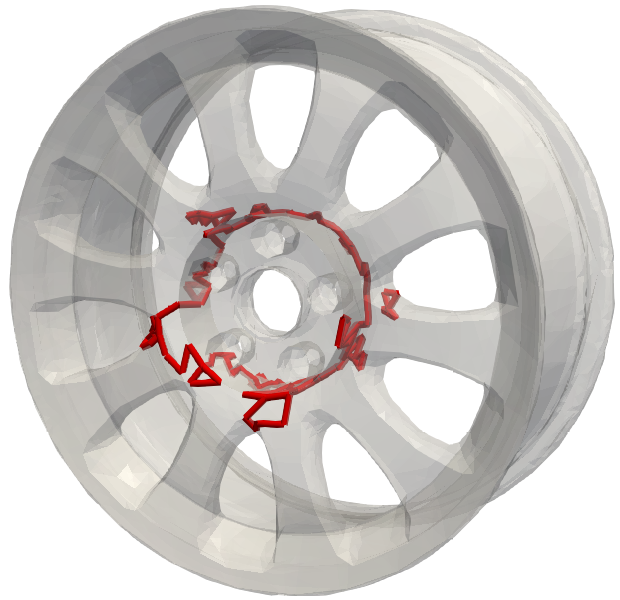
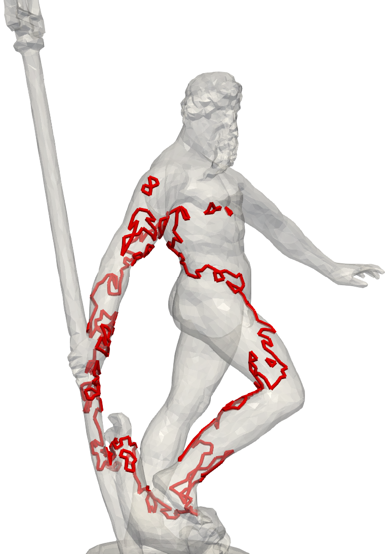
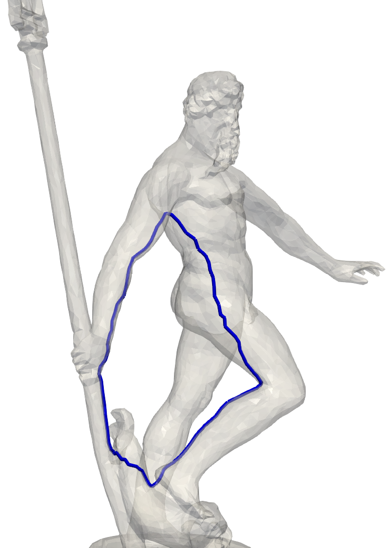
Figure 5: The localization algorithm computes optimal (blue) 1-cycles that are homologous to input 1-cycles (red).

D.2 Optimal homology basis

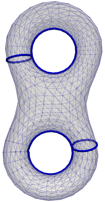
Figure 6: Optimal 1-homology basis computed using the localization algorithm.

D.3 Optimal Persistent Homology Representatives

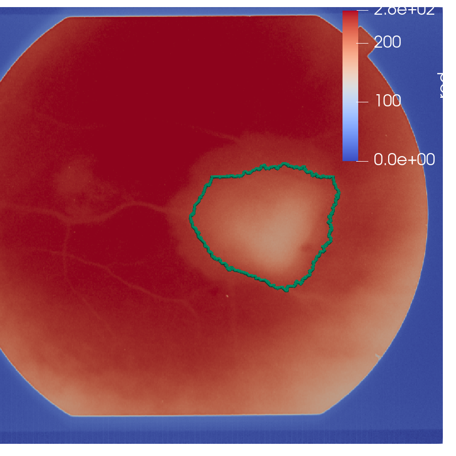
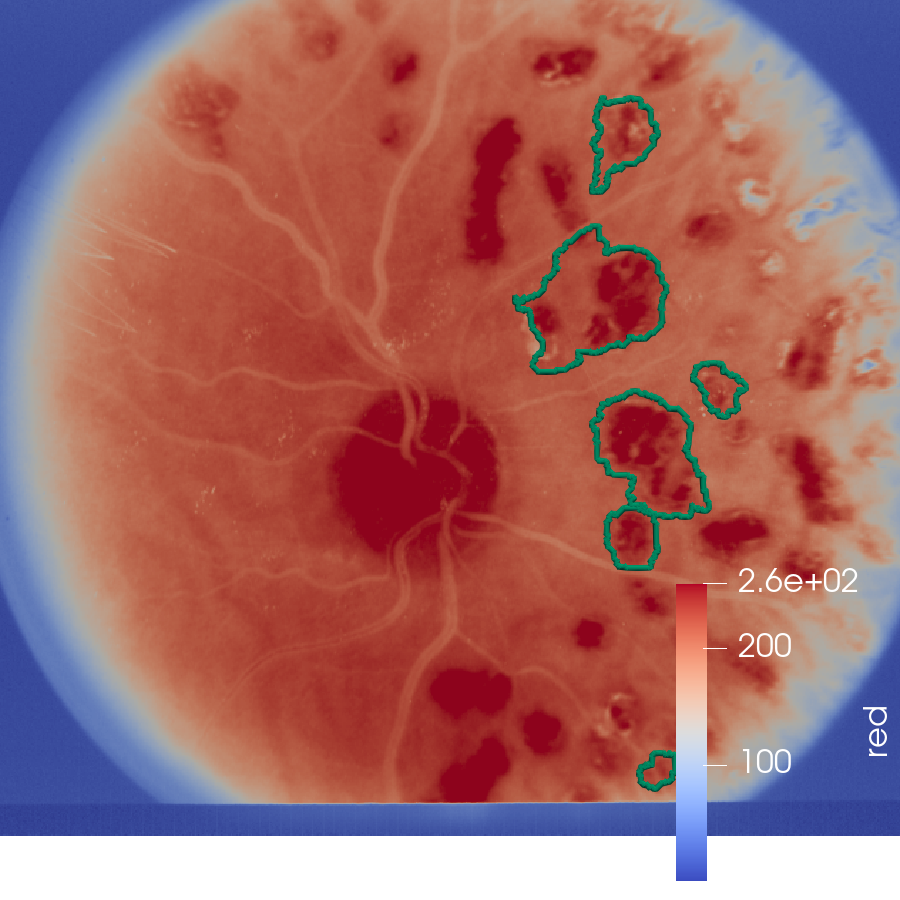
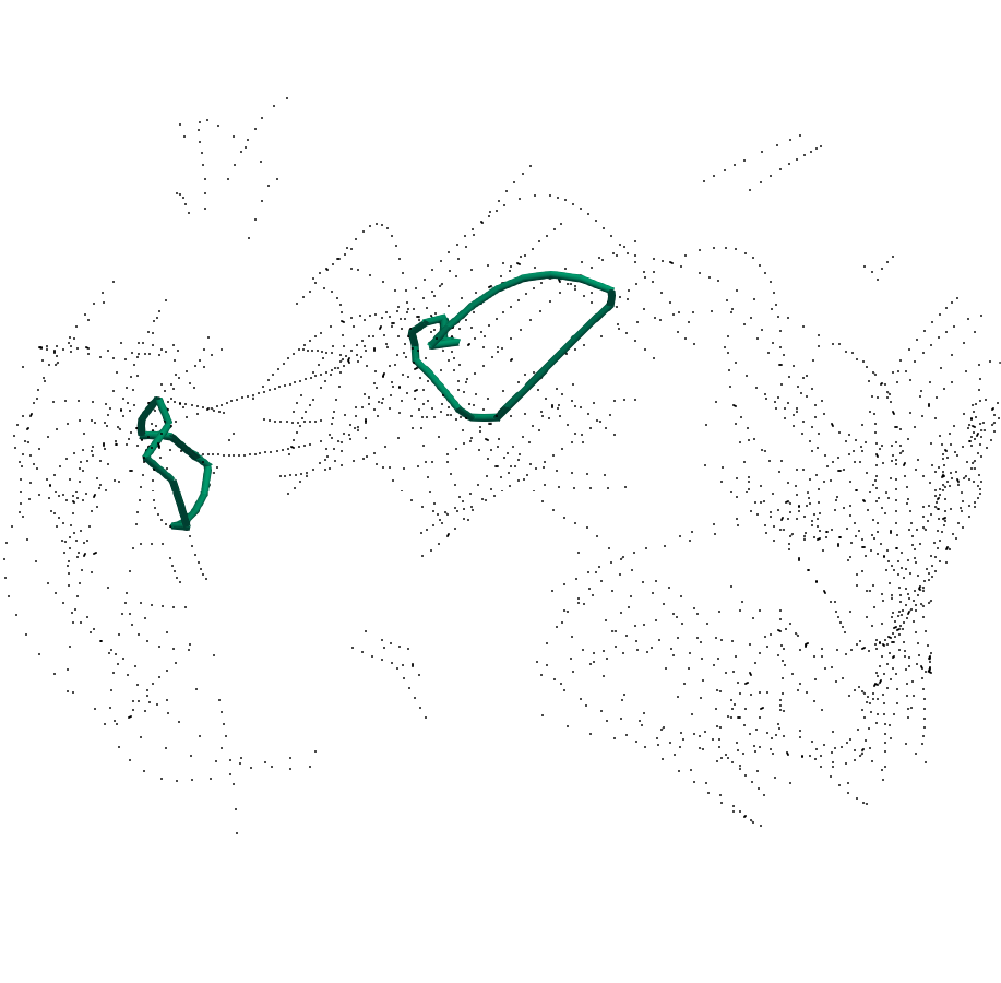
(a)	(b)	(c)

Figure 7: (a)Persistent homology representative of longest bar bounding a region of disorder in the retinal image. (b) Representatives of few of the top-most bars indicating regions of disorder in the retinal image. (c) Top 2 representatives of the Lorenz’96 dataset(20%)

References

- [1] H. Bakke Bjerkevik. On the stability of interval decomposable persistence modules. Discrete & Computational Geometry, 66(1):92–121, 2021.
- [2] A. Barbensi, I. H. R. Yoon, C. D. Madsen, D. O. Ajayi, M. P. H. Stumpf, and H. A. Harrington. Hypergraphs for multiscale cycles in structured data, 2022.
- [3] U. Bauer, M. Kerber, J. Reininghaus, and H. Wagner. PHAT–persistent homology algorithms toolbox. Journal of symbolic computation, 78:76–90, 2017.
- [4] G. Borradaile, E. W. Chambers, K. Fox, and A. Nayyeriy. Minimum cycle and homology bases of surface-embedded graphs. Journal of Computational Geometry, 8(2), 2017.
- [5] G. Borradaile, W. Maxwell, and A. Nayyeri. Minimum bounded chains and minimum homologous chains in embedded simplicial complexes. In 36th International Symposium on Computational Geometry, SoCG 2020, volume 164 of LIPIcs, pages 21:1–21:15, 2020.
- [6] M. Botnan. Mastermath course topological data analaysis. http://www.few.vu.nl/~botnan/lecture_notes.pdf, 2022.
- [7] E. W. Chambers, J. Erickson, and A. Nayyeri. Minimum cuts and shortest homologous cycles. In Proceedings of the twenty-fifth annual symposium on Computational geometry, pages 377–385. ACM, 2009.
- [8] E. W. Chambers, S. Parsa, and H. Schreiber. On complexity of computing bottleneck and lexicographic optimal cycles in a homology class. In 38th International Symposium on Computational Geometry, SoCG 2022, volume 224 of LIPIcs, pages 25:1–25:15, 2022.
- [9] C. Chen and D. Freedman. Measuring and computing natural generators for homology groups. Computational Geometry, 43(2):169–181, 2010.
- [10] C. Chen and D. Freedman. Hardness results for homology localization. Discrete & Computational Geometry, 45(3):425–448, 2011.
- [11] D. Cohen-Steiner, A. Lieutier, and J. Vuillamy. Lexicographic optimal homologous chains and applications to point cloud triangulations. In 36th International Symposium on Computational Geometry, SoCG 2020, volume 164 of LIPIcs, pages 32:1–32:17, 2020.
- [12] D. Cohen-Steiner, A. Lieutier, and J. Vuillamy. Lexicographic optimal homologous chains and applications to point cloud triangulations. Discrete & Computational Geometry, pages 1–20, 2022.
- [13] T. K. Dey, A. N. Hirani, and B. Krishnamoorthy. Optimal homologous cycles, total unimodularity, and linear programming. SIAM Journal on Computing, 40(4):1026–1044, 2011.
- [14] T. K. Dey, T. Hou, and S. Mandal. Persistent 1-cycles: Definition, computation, and its application. In International Workshop on Computational Topology in Image Context, pages 123–136. Springer, 2019.
- [15] T. K. Dey, T. Hou, and S. Mandal. Computing minimal persistent cycles: Polynomial and hard cases. In Proceedings of the Fourteenth Annual ACM-SIAM Symposium on Discrete Algorithms, pages 2587–2606. SIAM, 2020.
- [16] T. K. Dey, J. Sun, and Y. Wang. Approximating loops in a shortest homology basis from point data. In Proceedings of the Twenty-Sixth Annual Symposium on Computational Geometry, pages 166–175. ACM, 2010.
- [17] T. K. Dey and Y. Wang. Computational Topology for Data Analysis. Cambridge University Press, 2022. https://www.cs.purdue.edu/homes/tamaldey/book/CTDAbook/CTDAbook.pdf.
- [18] H. Edelsbrunner and J. Harer. Computational Topology: An Introduction. Applied Mathematics. American Mathematical Society, 2010.
- [19] H. Edelsbrunner, D. Letscher, and A. Zomorodian. Topological persistence and simplification. Discrete Comput. Geom., 28:511–533, 2002.
- [20] J. Erickson and K. Whittlesey. Greedy optimal homotopy and homology generators. In Proceedings of the sixteenth annual ACM-SIAM symposium on Discrete algorithms, pages 1038–1046. Society for Industrial and Applied Mathematics, 2005.
- [21] P. Gabriel. Unzerlegbare Darstellungen I. Manuscripta Mathematica, 6(1):71–103, 1972.
- [22] G. Henselman-Petrusek. personal communication.
- [23] A. Hoover and M. Goldbaum. Locating the optic nerve in a retinal image using the fuzzy convergence of the blood vessels. IEEE Transactions on Medical Imaging, 22(8):951–958, 2003.
- [24] L. Li, C. Thompson, G. Henselman-Petrusek, C. Giusti, and L. Ziegelmeier. Minimal cycle representatives in persistent homology using linear programming: An empirical study with user’s guide. Frontiers in artificial intelligence, 4:681117, 2021.
- [25] I. Obayashi. Volume-optimal cycle: Tightest representative cycle of a generator in persistent homology. SIAM Journal on Applied Algebra and Geometry, 2(4):508–534, 2018.
- [26] I. Obayashi. Stable volumes for persistent homology. Journal of Applied and Computational Topology, 7(4):671–706, 2023.
- [27] A. Rathod. Fast algorithms for minimum cycle basis and minimum homology basis. In 36th International Symposium on Computational Geometry, SoCG 2020, volume 164 of LIPIcs, pages 64:1–64:11, 2020.
- [28] Sayan Mandal, Tamal K Dey , Tao Hou. "persloop software for computing persistent 1-cycle. https://github.com/Sayan-m90/Persloop-viewer.
- [29] K. Strommen, M. Chantry, J. Dorrington, and N. Otter. A topological perspective on weather regimes. Climate Dynamics, 60:1–31, 07 2022.