Reconstructing training data from document understanding models

Abstract

Document understanding models are increasingly employed by companies to supplant humans in processing sensitive documents, such as invoices, tax notices, or even ID cards. However, the robustness of such models to privacy attacks remains vastly unexplored.

This paper presents CDMI, the first reconstruction attack designed to extract sensitive fields from the training data of these models. We attack LayoutLM and BROS architectures, demonstrating that an adversary can perfectly reconstruct up to 4.1% of the fields of the documents used for fine-tuning, including some names, dates, and invoice amounts up to six-digit numbers. When our reconstruction attack is combined with a membership inference attack, our attack accuracy escalates to 22.5%.

In addition, we introduce two new end-to-end metrics and evaluate our approach under various conditions: unimodal or bimodal data, LayoutLM or BROS backbones, four fine-tuning tasks, and two public datasets (FUNSD and SROIE). We also investigate the interplay between overfitting, predictive performance, and susceptibility to our attack. We conclude with a discussion on possible defenses against our attack and potential future research directions to construct robust document understanding models.

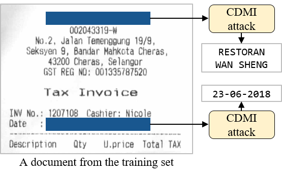
Figure 1: A document (licensed CC BY 4.0 DEED by [35]) where two fields are perfectly reconstructed by CDMI. A model with LayoutLM architecture [81] is trained on SROIE dataset [35]. Then, when the date or the company is scrubbed, the adversary is able to reconstruct it.

1 Introduction

Document understanding models aim at processing visually rich documents, such as handwritten forms, tax invoices or scanned tables, where information is encoded both in textual content and layout. Consequently, most document understanding models adapt a language model architecture to make it layout-aware [81, 80, 34, 32, 25, 62]. These models have countless real-world applications and are employed by numerous companies for tasks extending from key information extraction [51, 34, 60] to document classification [57, 29], and question answering [77, 53].

Moreover, a range of neural network architectures have been found vulnerable to membership inference or reconstruction attacks in multiple domains: computer vision models [24, 23, 87, 44, 42, 76], language models [86, 9, 8, 46, 68, 50, 55, 47], graph models [88, 58], and diffusion models [7], among the most popular. Those attacks enable an adversary to obtain information on the training data, posing a serious threat to confidentiality (see section 2.2 and [69, 67]).

Surprisingly, despite their resemblance to language models and vision models, we have not discovered any existing studies on the robustness of document understanding models to such privacy attacks (at the time of writing, in October 2023). The most related research paper we found in this domain is by [54]. However, they define a document as a collection of sentences, excluding any layout information. Thus, the model they target (Sentence-BERT [64]) differs significantly from state-of-the-art document understanding models. The reconstruction attack we present in this paper is the first to target some of the most commonly used layout-aware models and treat documents as multimodal data.

1.1 Contributions

Our main contributions are as follows:

• We develop the first reconstruction attack that targets layout-aware document understanding models: a white-box attack named CDMI (Combinatorial Document Model Inversion), designed to target unimodal or bimodal models. We employ CDMI to reconstruct fields from the fine-tuning datasets of our models, although it is also readily adaptable for pre-training datasets.

• We combine CDMI with existing membership inference attacks, resulting in an end-to-end attack where the adversary extracts arbitrary fields in the training dataset.

• We introduce two new end-to-end metrics to evaluate simultaneously the reconstruction and the membership inference attack. Our intention is to evaluate the full extent of potential harm that an adversary could cause.

• We successfully evaluated our attack in various settings, making it one of the few attacks capable of reconstructing non-synthetic data from an encoder-only model. These settings include unimodal or bimodal models, with either LayoutLM v1 [81] or BROS [32] backbone, using four different training tasks, and two public fine-tuning datasets: FUNSD [40] and SROIE [35].

• We demonstrate that the success of our attack is not due to over-fitting or data duplication, and that memorization occurs early in the training pipeline. We also prove that both the layout and the visual modality contribute to memorization, proving that documents should be considered as a specific data type with dedicated attacks.

2 Background and related work

2.1 Document understanding models

A document processing pipeline aims at extracting meaningful information from raw document images such as scans, pictures, or screenshots. Deep learning-based pipelines usually include two main steps [71]:

• An Optical Character Recognition (OCR) is used to extract the textual content of the document: its output typically includes words and their associated bounding boxes, which denote the coordinates of the four points encompassing the word. Then, the words are fed to a tokenizer. It splits the words into tokens, which are smaller pieces of text that are part of a specific vocabulary.

• These tokens and their bounding boxes are processed by a document understanding model, which extracts specific information from them. A model is said to be layout-aware when it uses both the tokens and the layout information derived from the bounding boxes [77].

The architectures we target: LayoutLM v1 and BROS

Recently, OCR-free pipelines were developed [14, 27, 10, 45]. However, our focus will be on deep learning models specifically designed to work with an OCR, given that OCR-free approaches are relatively new and rarely deployed in production. The category of OCR-based models includes recent architectures with state-of-the-art results such as LayoutLM v1 [81], LayoutLM v2 [80], LayoutLM v3 [34], BROS [32], LAMBERT [25], TILT [62], and DocFormer [4].

We decided to attack two different architectures: LayoutLM v1 and BROS, for multiple reasons. Firstly, both architectures demonstrate strong performance and are frequently used in real-world applications. In addition, their pretrained weights are available under permissive licenses (in contrast to LayoutLM v3), making them particularly suitable for commercial applications. Thus, "LayoutLM" will implicitly refer to LayoutLM v1 in the following.

Transformer-based document encoders

These architectures are transformer-based encoder-only models, akin to BERT [13]. They employ multiple layers of multi-headed Transformers [74] to embed each input token in a feature space of dimension $d=768$. However, unlike BERT, these architectures use a 2-dimensional spatial encoding to consider the layout information provided by the bounding boxes.

In addition to the tokens and their bounding boxes, a document understanding model can exploit the raw images of the documents [81, 62, 32]. In the case of LayoutLM and BROS, visual features are generated by a computer vision model, and subsequently added to the textual embedding of each token using Region Of Interest alignment [30]. We will refer to these models as bimodal, in contrast to the simpler layout-aware models which we will refer to as unimodal.

Training objectives

LayoutLM and BROS encoders are often used in a transfer learning setting. First, the encoders are pre-trained on a very large corpus of documents, the IIT-CDPI Test Collection 1.0 [49]. The main pre-training task is Masked Language Modeling (MLM), where approximately 15% of the tokens are masked, and the model is trained to reconstruct them. Afterwards, the model is fine-tuned on a specific task by keeping the pretrained backbone and replacing the last layers with a new classification head specifically designed for this task. Our attack will target these fine-tuned models.

We evaluated our attack against models fine-tuned on three common Key Information Extraction (KIE) tasks, which were previously employed by [32] to evaluate BROS:

• Entity Extraction with BIO tagging (EE-BIO): it aims at extracting some fields of the document by classifying its tokens as "Beginning", "Inside" or "Out" of an entity [3].

• Entity Extraction with SPADE tagging (EE-SPADE or EE-SPD): it also aims at extracting some fields using the SPADE tagging [36]. In a nutshell, the model is trained to identify the predecessor of each token in the entities of the document.

• Entity Linking (EL): it aims at establishing connections between the entities using their semantic relations. We also used SPADE tagging for this task [36].

In addition to those three tasks, we also attacked models that were fine-tuned on the same MLM task that is utilized during pre-training. This scenario does not correspond to a real-world setting; however we did this to compare the susceptibility of the KIE and the MLM tasks under the same conditions (transfer learning with the same fine-tuning dataset, etc.). All these tasks ultimately involve a token-level classification task, for which we used a cross-entropy loss.

2.2 Privacy attacks

In this section, we introduce privacy attacks and review the existing ones in the field of Natural Language Processing (NLP). Indeed, the architectures of language models are similar to those of document understanding models, for which such attacks have not yet been studied.

Taxonomy

Various types of attacks target the confidentiality of models trained on sensitive data by exploiting unintended memorization of their training set. Following [50], we distinguish three levels of privacy attacks:

• Extraction attacks: the adversary has only access to the model, and seeks to extract as much data as feasible from the training set. In NLP, such attacks are studied in [9, 8, 46, 68, 50, 86, 84].

• Reconstruction attacks: the adversary has access to a model and a context such as the prefix of a sentence, or a document with a scrubbed field, and seeks to reconstruct the missing parts. In NLP, attacks of this kind include [50, 59, 19, 54].

• Membership inference attacks [69]: the adversary has access to data samples, and attempts to predict whether they are part of the model’s training set or not. Formally, this is equivalent to a reconstruction attack with a finite list of candidates for the reconstruction. Notable examples of these attacks are [55, 47, 70, 52, 66].

In this paper, we focus on reconstruction attacks. We begin with a ground truth document, represented for now as a sequence of tokens $d_{g}$ in a vocabulary $\mathcal{V}$. A field is scrubbed by replacing it with the special token [MASK] to form $\widetilde{d_{g}}$. Then, the adversary has access to $\widetilde{d_{g}}$ and optimizes equation 1 to reconstruct the scrubbed fields.

$$\operatornamewithlimits{argmax}_{d\in\mathcal{V}^{*}}\ P_{\theta}(d\ |\ \widetilde{d_{g}})$$ (1)

Here, $P_{\theta}$ denotes the likelihood of $d$ being a good reconstruction of $\widetilde{d_{g}}$ given the model’s weights $\theta$. However, this probability is frequently either ill-defined or intractable. Hence, practical attacks necessitate the construction of a suitable proxy for $P_{\theta}$ (see [50] and sections 4.1 and 4.2).

Attacks against decoder-only models

In the context of extraction and reconstruction attacks in NLP, a significant difference exists between decoder-only models and others [37, 82]. Decoder-only models, such as the ones of the GPT family, are trained in an auto-regressive way to generate the next token in a sequence given its prefix. They are well-designed to generate fluent content.

Existing attacks against such models directly use this generation ability to extract training data [9, 8, 46, 50, 84]. These attacks reconstruct data from left to right. At step $t$, using the previously reconstructed prefix sequence $\widetilde{s_{g}}=c_{1}\dots c_{t-1}$, they attempt to reconstruct token $c_{t}$ . As a result, if they directly replace $P_{\theta}$ by the probability distribution calculated by the model for the next token, equation 1 ends up being exactly the one the model is trained to solve:

$$\operatornamewithlimits{argmax}_{c_{t}\in\mathcal{V}}\ P_{\theta}(c_{t}\ |\ c_{1},\dots,c_{t-1})$$ (2)

Attacks against encoder-only model

Encoder-only models, such as LayoutLM or BROS, are not designed to compute a probability distribution over sentences. This makes it difficult for them to generate fluent content [75, 26]. This is a crucial difference, because this ability is needed to reconstruct plausible content in equation 1. However, various strategies have been proposed to attack encoder-only models in NLP:

• [86] employ an auxiliary GPT-2 model [6] to generate content. They utilize the PPLM mechanism [12] to increase the likelihood of generating content from the training set of the BERT model they target [13].

• [47] focus on small prompts in a clinical context, and conclude that their attack does not significantly expose the training data. [55] enhance their attack in a membership inference setting, adopting the energy-based interpretation of [26] instead of Gibbs sampling to compute text fragment likelihoods.

• [8] assess their attack against T5 model [63]. However, they addressed a simpler scenario where it is not needed to generate fluent content: 15% of randomly chosen tokens are masked and need to be reconstructed.

• [70] and [59] formulate a continuous relaxation of equation 1 inspired from the work of [38] for its resolution.

• [52] target embedding models, exploiting specific properties of these models in their attack.

• [19] focus on canary reconstruction and use an autoregressive proxy. They decode tokens from left to right, with the objective of minimizing the loss of the model. [20] improves the approach of [19] by using a MLM head to select candidates before evaluating the loss of the target model.

• [54] only focus on differential privacy [17, 18, 16, 1], demonstrating theoretical privacy bounds without implementing the attack to test these limits.

Thus, reconstructing training data from encoder-only models is a difficult task, and there is no standard method for it. To attack real-world document understanding models, we could not directly apply existing methods. Indeed, they either constituted membership inference attacks (which are less complex than reconstructions) [47, 55], were only evaluated on frequently repeated canaries [20, 19, 59], or were inapplicable to our scenario [52, 8, 54, 70].

We selected and combined promising ideas from various existing attack, improving and optimizing them for our scenario. We utilized an autoregressive proxy as in [19, 20], and leveraged an auxiliary generator to enhance the fluency of the reconstructions as in [86, 20]. We also developed a customized method for incorporating the loss of the target model, which we combined with existing membership inference metrics [9]. Finally, we integrated the visual modality in our attack to extract information memorized by the visual encoder. This led to our hybrid attack, CDMI, the first of its kind capable of reconstructing real documents.

Defense against privacy attacks

According to [37], the main defense techniques in a centralized setting are:

• Data sanitization [65, 11, 73, 5]. It involves removing personal data from the training set. However, this technique is limited due to the context-dependent definition of personal data [5]. Deduplication, which consists in eliminating duplicate data, can also be useful as duplicated data is more likely to be memorized [43].

• Differential Privacy (DP) [17, 16, 18, 1]. This training paradigm adds noise to each gradient during the training phase up to a certain level, to safeguard every sample in the training set. However, the effectiveness of DP in genuine real-world settings is disputed [15, 72].

• Regularization. Although not necessary, overfitting facilitates the memorization of training data [83, 85, 21, 9]. Hence, some mechanisms involving regularization have been proposed [56, 33].

• Post-processing. Confidence masking and output filtering can be employed during post-processing [23, 61].

3 Threat model

In this section we introduce our threat model, which defines the assumptions we made for the development of our attack.

3.1 Adversarial capabilities and goals

We make two primary assumptions about the adversary’s capabilities:

• White box hypothesis. The adversary is supposed to have white-box access to the model, meaning complete access to its architecture and weights. Concretely, our attack is gradient-free, but because it requires computing the token-level loss for a large number of inputs, it is impractical in standard black-box environments. This is why we classify it as a white-box attack.

• Scrubbed data. Given that we are developing a reconstruction attack, we assume the adversary has access to scrubbed data. In our context, this means that the adversary can access a document (token, bounding boxes, and the raw image) where a certain field has been masked (tokens replaced by [MASK], and a white patch to replace the field in the image). This implies that the adversary knows the number of tokens in the target field. While this is a strong supposition, it is necessary to make our optimization in equation 1 tractable (see III.B in [50]). Moreover, this assumption is fairly realistic for documents in which the fields adhere to strict rules (e.g. IBANs, credit card number and expiration date, etc.).

We focus on an adversary whose goal is to reconstruct the textual modality of documents, regardless of whether the target model is unimodal or bimodal. Indeed, for real-world document understanding models, sensitive information is often encoded in the textual modality. For example, for identity theft, reconstructing the ID card number and expiration date is significantly more valuable than the general layout of the card, which is common knowledge.

More specifically, we distinguish two variants of our attack, a one-shot one and a multi-shot one, each with slightly different adversarial goals:

• One-shot variant. In this scenario, the adversary makes one reconstruction attempt per field in the datasets. Here, their objective is to maximise the similarity metrics between their reconstruction and the ground truth.

• Multi-shot variant. This setting is closer to a real-world scenario. The adversary makes multiple attempts against each field, and ultimately uses a membership inference metric to filter the most plausible reconstructions, as referenced in [9, 84]). The adversary has two objectives. First, to generate high-quality reconstructions. Second, to accurately retain the correct ones using the membership inference metric (see section 5.3).

3.2 The reconstruction game

Notation	Description
$\mathcal{T}$	A stochastic training procedure
$\mathcal{A}$	A procedure denoting an adversary
$\mathcal{V}$	The vocabulary for the tokens
$\mathcal{I}=\mathbb{R}^{3\times d_{i}}$	The RGB space of documents’ images
$D\sim\mathcal{D}^{n}$	Sample $n$ docs from a distribution $\mathcal{D}$ on $\mathcal{V}^{*}\times\mathcal{I}$
$d\in\mathcal{V}^{*}\times\mathcal{I}$	A document (sequence of tok. + image)
$\widetilde{d}\in\mathcal{V}^{*}\times\mathcal{I}$	A scrubbed document derived from $d$
$y\in\mathbb{R}^{*}$	A classification label for a document
$f\in\mathcal{V}^{*}$	A field of $d$ containing personal info.
$\widetilde{f}\in\mathcal{V}^{*}$	A reconstruction attempt for $f$
$k=|f|$	The number of tokens in $f$

Table 1: Notations

Following [67, 79], we define the reconstruction game, that serves to formalize the threat model, the information the adversary can access, and what will be used for evaluation. It is an adaptation of the one in [50]. In addition to the notations of table 1, we define:

• $\text{EXTRACT}(d)$: extracts the list of fields of $d$ that contain personal information.

• $\text{SCRUB}(d,f)\rightarrow\widetilde{d},y$: scrubs a field $f$ in a document $d$ by replacing it by [MASK], and returns its classification label $y$ (which is public information).

Our multi-shot reconstruction game is presented in algorithm 1. Initially, a model is trained on a private dataset $D$ (lines 2–3). Then, for each document in the dataset (line 6), and for each field in this document (line 7), the field is scrubbed and the adversary attempts $n_{a}$ reconstructions (lines 8–12). The adversary has access to the ground truth number of tokens $k$ (see section 3.1). They also know $\mathcal{D}$, $\mathcal{T}$, and $n$, which means they can train auxiliary models on the same distribution. Then, a Membership Inference (MI) metric is utilized to keep the best reconstruction attempt for each field (line 13). Subsequently, the MI metric is used to sort the fields by probability of successful reconstruction (line 16). Finally, we evaluate the attempts, examining both their similarity to their ground truth, and their order with respect to the MI metric computed at line 16 (see section 5.3).

The one-shot reconstruction game is very similar. Since there is only one attempt per scrubbed field, lines 9, 10, 12, 13 are removed. Furthermore, the order of the fields is not considered during evaluation, so line 16 is removed.

With these notations, we can refine equation 1 introduced earlier. At line 11, the adversary seeks to solve equation 3. We recall that the adversary only tries to reconstruct the textual modality of the fields, which is why the optimization is over $\widetilde{f}\in\mathcal{V}^{k}$ and not over $\widetilde{f}\in\mathcal{V}^{k}\times\mathcal{I}$ (see section 3.1 and the paragraph on visual modality in section 4.1).

$$\mathcal{A}(\mathcal{T},\mathcal{D},n,\theta,\widetilde{d},y,k)=\operatornamewithlimits{argmax}_{\widetilde{f}\in\mathcal{V}^{k}}\ P_{\theta}(\widetilde{f}\ |\ \widetilde{d},y)$$ (3)

Algorithm 1 The multi-shot reconstruction game

1:experiment RECON_M_SHOT($\mathcal{D},\mathcal{T},\mathcal{A},n$)

2: Sample docs and train a model

3:     $D\sim\mathcal{D}^{n}$

4:     $\theta\leftarrow\mathcal{T}(D)$

5:     $F\leftarrow[\ ]$

6:     $\widetilde{F}\leftarrow[\ ]$

7: $n_{a}$ reconstruction attempts on each field

8:     for $d\in D$ do

9:         for $f\in\text{EXTRACT}(d)$ do

10:              $\widetilde{d},y\leftarrow\text{SCRUB}(d,f)$

11:              $\text{attempts}\leftarrow[\ ]$

12:              for $a\in[1,\dots,n_{a}]$ do

13:                  $\widetilde{f}\leftarrow\mathcal{A}(\mathcal{T},\mathcal{D},n,\theta,\widetilde{d},y,k)$

14:                  $\text{attempts}\leftarrow\text{CONCAT}(\text{attempts},[\ \widetilde{f}\ ])$               

15: MI to keep one attempt per field

16:              $\widetilde{f}\leftarrow\text{MI\_FILTER}(\text{attempts})$

17:              $F\leftarrow\text{CONCAT}(F,[\ f\ ])$

18:              $\widetilde{F}\leftarrow\text{CONCAT}(\widetilde{F},[\ \widetilde{f}\ ])$               

19: MI to sort reconstructions by plausibility

20:     $F,\widetilde{F}\leftarrow\text{MI\_SORT}(F,\widetilde{F})$

21:     $\text{EVAL}(F,\widetilde{F})$

3.3 Ethical considerations

This paper presents an attack that specifically targets the privacy of document understanding models. This raises ethical considerations because such models are sometimes trained on private data and used in real-world settings.

First, we reduce ethical concerns by only attacking models trained on publicly-available data: LayoutLM v1 [81] and BROS [32] are both pre-trained on the public dataset IIT-CDIP Test Collection 1.0 [49]. Moreover, we fine-tune them on two other public datasets, FUNSD [40] and SROIE [35].

Moreover, our attack still necessitates a substantial amount of prior information to successfully reconstruct data. As for every reconstruction attack, this includes access to scrubbed data, an uncommon scenario. Consequently, while our approach may set the foundation for more efficient methods with less information, we argue that the advantages of disclosing it outweigh potential harm. Researchers and companies training document understanding models on private data must understand that robust attacks are very likely to exist in the future. Therefore, it is crucial they protect access to their trained models with the same stringency as their databases.

Finally, we believe that disclosing our attack is important to shed light on privacy attacks and ensure they are considered by institutional regulators. Currently, despite the development of attacks on numerous model types, the fact that trained models may leak personal information is frequently overlooked in data regulation texts such as RGPD and AI Act in European Union, APPI in Japan, CCPA in California, etc.

4 The CDMI reconstruction method

The section details the methodology employed for our reconstruction attack: CDMI (Combinatorial Document Model Inversion). Specifically, it elaborates on three aspects: the chosen proxy for $P_{\theta}$ in equation 3; how we optimize it; and the membership inference metric we used.

In summary, our attacks proceeds as follows. First, we approximate the probability distribution over the fields using an autoregressive proxy, meaning that tokens will be reconstructed from left to right within each field (see section 4.1). To reconstruct each token, we compute and optimize a token-level probability $P_{\theta}^{\text{tok}}$ (see section 4.2). For this, we employ a masked model trained on public data to select candidates. Next, we evaluate the loss of the target model for each candidate, using these computations to approximate $P_{\theta}^{\text{tok}}$. Finally, we sample the reconstruction from this approximate distribution. We also present two variants of our attack: the one-shot one, and the multi-shot one, where the adversary attempts several reconstructions against each field and selects the best one using a membership inference metric (see section 4.3).

4.1 An autoregressive proxy

To solve equation 3, the adversary needs to choose a convenient proxy for $P_{\theta}$, that should correctly represent the likelihood of a document being in the training set while being easy to optimize. Adapting the methodology of [19] in NLP, we employ an autoregressive formulation, meaning that scrubbed tokens are sequentially reconstructed from left to right.

Equation 4 presents this autoregressive proxy, with notations derived from table 1. We recall that $k$, the number of tokens in the target field, is known to the adversary (see section 3.1). This formula employs a token-level proxy $P_{\theta}^{\text{tok}}$, that represents the probability that the selection of token $v_{t}\in\mathcal{V}$ at step $t$ results in a good reconstruction.

$$P_{\theta}(\widetilde{f}\ |\ \widetilde{d},y)\ =\ \prod_{t=1}^{k}P_{\theta}^{\text{tok}}(v_{t}\ |\ \widetilde{d},y,v_{1},\dots,v_{t-1})$$ (4)

Although encoder-only models such as LayoutLM or BROS are not designed for such an autoregressive formulation [75, 26], we used this approximation for several reasons:

• This autoregressive modeling substantially decreases the size of the search space. Rather than $\mathcal{V}^{k}$, our optimization problem is divided into $k$ sub-problems in $\mathcal{V}$.

• More complex methods require a significantly higher number of model calls [26]. Considering that our attack is already computation-intensive, our autoregressive proxy serves to maintain this number to a minimum.

• The left-to-right decoding is requisite for the SPADE [36] implementation we used. Indeed, each token is trained to point towards its predecessor, thereby making it significantly easier to decode if the predecessor has already been reconstructed.

• Using an autoregressive decoding enables us to use various heuristics derived from reconstruction attacks on decoder-only models [84].

As explained in section 2.1, our attack targets both unimodal (text + layout) and bimodal (text + layout + image) models. Nevertheless, the objective of the adversary is solely to reconstruct the textual data (see section 3.1). When attacking a bimodal model, we did the following:

• To scrub bimodal data, target tokens are replaced with [MASK] token, and a white patch masks the content of the field in the image.

• With our autoregressive proxy, we sequentially replace the target tokens with their reconstruction in the textual modality.

• The visual modality remains masked throughout the entire field reconstruction process. This means that the white patch masks all tokens, and remains unchanged even when the initial ones have already been reconstructed in the visual modality. Indeed, the adversary makes no attempt to reconstruct the visual modality (cf. section 3.1), even when attacking a bimodal model.

This is why our equations only optimize on $\mathcal{V}^{k}$. The information of the image $\mathcal{I}$ comes from the scrubbed document $\widetilde{d}\in\mathcal{V}^{*}\times\mathcal{I}$.

4.2 A token-level combinatorial optimization

The computation and optimization of $P_{\theta}^{\text{tok}}$ involves several steps that are shown in algorithm 2 and figure 2. In essence, we leverage an auxiliary MLM head trained on public data to choose a list of potential tokens for reconstruction. Then, we compute the loss of the target model for each candidate, and select the one leading to the minimal loss. This is why we refer to our attack as combinatorial. Unlike the continuous relaxation used in NLP by [59, 70], we use discrete optimization by testing each candidate.

Details on step 1 (lines 2–4 in algo. 2, block A in fig. 2)

This step employs an auxiliary MLM head trained with $\mathcal{T}$ and $\mathcal{D}$. These are assumed to be public knowledge, hence this head is referred to as PUB-MLM. The step consists in a single forward-pass of the document in PUB-MLM, followed by the selection of the top-$N_{c}$ most plausible candidates.

This first step is needed because we empirically observed that the token minimizing the loss of the target model is often not the one we seek (e.g. unexpected words like "paranoia" for a "date" field). This was not an issue for [19] because they attacked canaries, whose structure is exactly known. However, for real data, we deem it necessary to initially filter plausible tokens with a MLM head.

Moreover, a forward-pass is executed for each candidate token during step 2. As such, selecting only a reasonable number of candidates significantly accelerates the attack.

Algorithm 2 Computing and maximizing $P_{\theta}^{\text{tok}}$

1:procedure $\operatornamewithlimits{argmax}_{v_{t}\in\mathcal{V}}\ P_{\theta}^{\text{tok}}$($v_{t}\ |\ \widetilde{d},y,v_{1},\dots,v_{t-1}$)

2: Getting candidates from auxiliary public MLM

3:     $[\ g_{i}\ ]_{1\leq i\leq|\mathcal{V}|}\leftarrow\text{MLM}_{\text{pub}}(\widetilde{d},v_{1},\dots,v_{t-1})$

4:     $[\ c_{i}\ ]_{1\leq i\leq N_{c}}\leftarrow\text{TOP}(N_{c},[\ g_{i}\ ]_{1\leq i\leq|\mathcal{V}|}).\text{indices}$

5:     $[\ g_{i}\ ]_{1\leq i\leq N_{c}}\leftarrow\text{TOP}(N_{c},[\ g_{i}\ ]_{1\leq i\leq|\mathcal{V}|}).\text{values}$

6: Computing target model loss

7:     $[\ l_{i}\ ]_{1\leq i\leq N_{c}}\leftarrow[\ \text{LOSS}(f_{\theta}(c_{i},y))\ ]_{1\leq i\leq N_{c}}$

8: Converting into likelihoods

9:     $[\ \widehat{g}_{i}\ ]_{1\leq i\leq N_{c}}\leftarrow\text{SOFTMAX}([\ g_{i}\ ]_{1\leq i\leq N_{c}})$

10:     $[\ \widetilde{l}_{i}\ ]_{1\leq i\leq N_{c}}\leftarrow 2-[\ l_{i}\ ]_{i}/\text{MEDIAN}([\ l_{i}\ ]_{i})$

11:     $[\ \widehat{l}_{i}\ ]_{1\leq i\leq N_{c}}\leftarrow\text{SOFTMAX}([\ \widetilde{l}_{i}\ ]_{1\leq i\leq N_{c}})$

12: Aggregating

13:     $[\ p_{i}\ ]_{1\leq i\leq N_{c}}\leftarrow[\ \text{MEAN}(\widehat{l}_{i},\widehat{g}_{i})\ ]_{1\leq i\leq N_{c}}$

14: Sampling with the final likelihoods

15:     $v_{t}\leftarrow\text{SAMPLE\_ONE}([\ p_{i}\ ]_{1\leq i\leq N_{c}})$

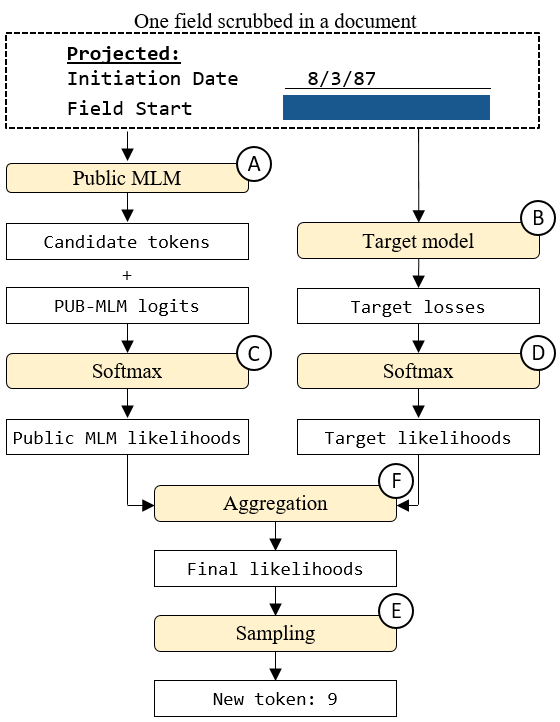
Figure 2: Computing and maximizing $P_{\theta}^{\text{tok}}$ to invert a token. We first use a masked model trained on public data to select $N_{c}=128$ candidates (A). Then, we compute the loss of the target model with each candidate (B), and aggregate these losses to obtain a probability distribution over the candidates (C, D, E). Finally, we sample the reconstructed token from this distribution (F), and repeat this process for the next tokens.

Details on step 2 (line 5 in algo. 2, block B in fig. 2)

For each of the $N_{c}$ candidate tokens, we execute a single forward-pass on the document, wherein the target token is replaced by the candidate token. These forward-passes can be arranged into one or several mini-batches depending on the available graphical memory. The loss applied is identical to the one used during training, which is the cross-entropy loss. However, we did not average over the mini-batch samples: $l_{i}$ corresponds to the loss for candidate token $c_{i}$, and to it alone.

The underlying idea is that the target model is trained to minimize the loss during training. Therefore, we assume that the loss is especially low for the specific token that was processed during training.

Details on step 3 (line 6 in algo. 2, block C in fig. 2)

This step involves converting the PUB-MLM logits into likelihoods using a softmax function. We incorporated two heuristics: a temperature parameter [22, 2], following the approaches of [9, 84, 46], and a decaying temperature as in [9], to promote the exploration of unexpected tokens only for the first tokens of the reconstruction.

Details on step 4 (lines 7–8 in algo. 2, block D in fig. 2)

This step involves the conversion of the losses of the target model into likelihoods. We must consider that:

• We want to minimize the loss (unlike the logits).

• We observed that the output loss usually consists in a majority of small values (e.g. of the order of $10^{-5}$), and some much larger outliers (e.g. of the order of $10^{0}$).

We used equation 5. First, losses are normalized by their median, attenuating the influence of the outliers. Then, we subtract the resulting value from $2$ to position the majority of values around $1$. Ultimately, a softmax function with decaying temperature is applied, as in step 3.

$$[\ \widehat{l}\ ]_{1\leq k\leq n}=\underset{1\leq j\leq N_{c}}{\text{SOFTMAX}}\left(2-\frac{l_{j}}{\text{MEDIAN}([\ l_{i}\ ])_{1\leq i\leq N_{c}}}\right)$$ (5)

Details on step 5 (line 9 in algo. 2, block E in fig. 2)

In this step, we integrate the PUB-MLM likelihoods with those of the target model. We explored two possibilities: an arithmetic weighted mean and a geometric weighted mean. Each of them offers distinct advantages. The arithmetic mean guarantees that both likelihoods always have the same relative importance, while the geometric means ensures that if one of the two likelihoods is exceptionally low, the mean will approach zero regardless of the other’s value. In practice, we opted for the geometric mean due to its superior results.

Details on step 6 (line 10 in algo. 2, block F in fig. 2)

Given the final likelihoods of the tokens, the remaining step consists of sampling one of them. This is a classical task in text generation [31]. Consistent with the results of [84, 46], we utilize top-$p$ sampling (also known as nucleus-$\eta$ [31]). The selection of parameter $p$ significantly influences the reconstructed field, and must be chosen in harmony with the temperature of the softmax functions.

4.3 Variants of the attack

Targeting a MLM head

As explained in section 2.1, we also target models trained on the MLM task, referred to as private MLM, unlike the PUB-MLM head which is used to optimize the token-level proxy (see section 4.2).

The attack method differs slightly when targeting such models, because we do not need to use another MLM as an auxiliary model. For steps 1 and 3, we replace the PUB-MLM head with the private MLM under attack. Then, we skip steps 2, 4 and 5, and directly utilize the likelihoods of the target model to sample the next token.

The multi-shot variant

For this variant, a membership inference metric is employed to sort the fields by plausibility of their reconstructions. In real-life scenarios, the adversary would set a threshold and only keep the most plausible ones.

Various membership inference metrics have been implemented in NLP [9, 46, 84, 47, 55]. Most of them rely on comparing the likelihood of a token or a sentence with respect to the target model and with respect to another model. Yet, computing the likelihood of a sentence for encoder-only models remains computationally intensive [55, 37]. Therefore we use the same approximation as for the reconstruction: computing the field likelihoods in an autoregressive manner:

• For each token $v_{t}$ in a field $\widetilde{f}$, we define its target likelihood as the probability $p_{i}$ it had during sampling at line 10 in algorithm 2. We also define its PUB-MLM likelihood as $\widehat{g_{i}}$, computed with the auxiliary MLM.

• We define the likelihood of a field as the product of the likelihoods of its tokens. We also use these token-level likelihoods to define the perplexity of a field [41].

While these definitions are approximations for encoder-only models, they offer the benefit of directly employing the PUB-MLM likelihood $\widehat{g_{i}}$ which is already computed during the attack. This circumvents the need for separate likelihood computation with an auxiliary model, as required in [55, 9, 84], except when targeting a private MLM head (see above). The five membership inference metrics we implement are:

• Raw perplexity: the PUB-MLM perplexity.

• Perplexity ratio: the ratio between the PUB-MLM perplexity and the target perplexity.

• Raw and ratio: the product of the two metrics above, aiming at prioritizing fields that have high PUB-MLM perplexity along with a high perplexity ratio.

• Max. token likelihood gap: the maximum difference between the private likelihood and the PUB-MLM one for every token (inspired from "high confidence" in [84]).

• Max. token likelihood ratio: similar to above, replacing the difference with a ratio.

5 Evaluation protocol

5.1 Datasets and training conditions

Dataset	Task	Acc LayoutLM		Acc BROS
		Unimod	Bimod	Unimod	Bimod
FUNSD	MLM	0.545	0.545	0.546	0.546
SROIE	MLM	0.540	0.538	0.541	0.539
FUNSD	EE-BIO	0.762	0.746	0.820	0.817
SROIE	EE-BIO	0.960	0.967	0.969	0.959
FUNSD	EE-SPD	0.760	0.760	0.815	0.804
SROIE	EE-SPD	0.952	0.935	0.965	0.965
FUNSD	EL	0.240	0.193	0.000	0.202

Table 2: The best validation accuracy of our models. For each of our 7 tuples (dataset, task), we trained unimodal and bimodal models with either LayoutLM or BROS backbone. These results are consistent with the one announced in [32]. For each of these 28 settings, we attacked both the model with the best validation accuracy (Precision criterion, presented here) and with the lowest validation loss (Loss criterion, presented in the appendix, see table 5).

Datasets

We evaluate the CDMI attack on models trained on two datasets: FUNSD [40] and SROIE [35], which are popular benchmarks for KIE tasks (see section 2.1). FUNSD consists of 199 scanned forms from the tobacco industry and includes annotations for both EE and EL tasks. We attack the fields annotated as "Anwers". For its part, SROIE incorporates 626 scanned receipts, only annotated for EE task. We attack the fields containing the date, company, address, and total amount. For both datasets, we only retain fields comprising between 3 and 15 tokens to disregard those that are either meaningless or too computationally demanding.

Each of our datasets is randomly partitioned into three non-overlapping parts (see appendix for details):

• A validation set, used to evaluate the generalization performance of models during their training phase.

• A private train set, comprising half of the remaining documents, and on which the models we target are trained.

• A public train set, containing the remaining documents, used to train auxiliary models.

Training conditions

We trained models in 28 different settings. For each of the 7 tuples (dataset, task) presented in table 2, we trained unimodal and bimodal models with either LayoutLM or BROS backbone. For each configuration, we trained our models for many epochs (300 for MLM tasks, 150 for the others), and saved the models at each epoch. Ultimately, we select the epoch we target with respect to one of the following criteria:

• Precision: the epoch with the best validation accuracy.

• Loss: the epoch with the best validation loss.

Using these 28 configurations and these 2 criteria, we evaluated both the one-shot and the multi-shot variant of our attack. This results in 112 different attack scenarios.

Hyperparameters: transferring from LayoutLM to BROS

The CDMI attack described in section 4 involves several hyperparameters: the number of candidates $N_{c}$ in step 1, the temperature parameter and decay in steps 3 and 4, the averaging method and its weight in step 5, the parameter $p$ for top-$p$ sampling in step 6, and the number of attempts $n_{a}$ for the multi-shot variant. We tuned these hyperparameters for the 14 configurations with LayoutLM backbone and Precision criterion, optimizing the evaluation metrics of the one-shot variant (see section 5.2 and the appendix).

Finally, we used each of these 14 sets of hyperparameters for 8 attacks: one-shot or multi-shot, Precision or Loss criterion, and LayoutLM or BROS backbone, yielding in a total of 112 evaluation settings. Given that the hyperparameters were calibrated with LayoutLM backbone, we anticipate the accuracy of CDMI to be superior with LayoutLM than with BROS. These enable us to assess the transferability of our attack, as we measure its performance on an architecture for which it was not optimized, namely BROS.

Hardware and computation time

Each of these 112 evaluations was performed on a fraction of 0.1 Nvidia A100 80GB. The mean computation time was 20:40 hours for each experiment, resulting in a total of about 2300 hours.

5.2 Evaluating the one-shot variant

Four evaluation metrics

To evaluate the quality of the one-shot attack, we compare each reconstruction $\widetilde{f}$ to its corresponding ground truth $f$. We employed four metrics for this purpose: the Perfect Reconstruction $\text{PR}=\mathbb{1}(f=\widetilde{f})$, the Hamming Distance (HD) [28], the normalized Levenshtein Distance (LD) [48], and the normalized Jaro-Winkler Distance (JWD) [39, 78]. We computed these metrics using the tokens of the fields, ignoring their alphanumeric decoding by the tokenizer, and we averaged them across all fields.

Our baseline

A logical analysis of the other fields and headers can often enable guessing many fields within a document. Consequently, we compare our one-shot attack to a baseline which represents the reconstruction that are feasible with public information only. In practice, this baseline corresponds to the reconstruction of the fields using only the PUB-MLM likelihoods in figure 2.

We compute the four evaluation metrics with this baseline, and compare them to our attack. In this way, we assess how useful it is to have access to the target model to obtain accurate reconstructions. Using an idea similar to the advantage often used in cryptography, we introduce the improvement factor (IpF), which represents the mean improvement between the attack and the baseline for our four metrics. For example, $\text{IpF}=1.5$ means that the attack is 50% better than the baseline on average. The improvement factor is defined in equation 6, where "att" represents the attack, and "base" the baseline. We also add a parameter $\varepsilon$ to bound the improvement factor.

$$\text{IpF}=\frac{\frac{\text{PR}_{\text{att}}+\varepsilon}{\text{PR}_{\text{base}}+\varepsilon}+\frac{\text{HD}_{\text{base}}+\varepsilon}{\text{HD}_{\text{att}}+\varepsilon}+\frac{\text{LD}_{\text{base}}+\varepsilon}{\text{LD}_{\text{att}}+\varepsilon}+\frac{\text{JWD}_{\text{base}}+\varepsilon}{\text{JWD}_{\text{att}}+\varepsilon}}{4}$$ (6)

5.3 Evaluating the multi-shot variant

The evaluation of the multi-shot variant must account for both the order of the reconstructions with respect to the membership inference metric ($F$ and $\widetilde{F}$), and the similarity between the fields and their reconstructions ($f_{i}\in F$ vs. $\widetilde{f_{i}}\in\widetilde{F}$). Thus, our evaluation metrics should satisfy the two following mathematical properties:

1. With fixed values $f_{i}$ and $\widetilde{f_{i}}$ for each $i$, the metric is maximized when $F$ and $\widetilde{F}$ are sorted in descending order of similarity between $f_{i}$ and $\widetilde{f_{i}}$.

2. With a fixed order of $F$ and $\widetilde{F}$, for each $i$, the metric increases when the similarity between $f_{i}$ and $\widetilde{f_{i}}$ increases.

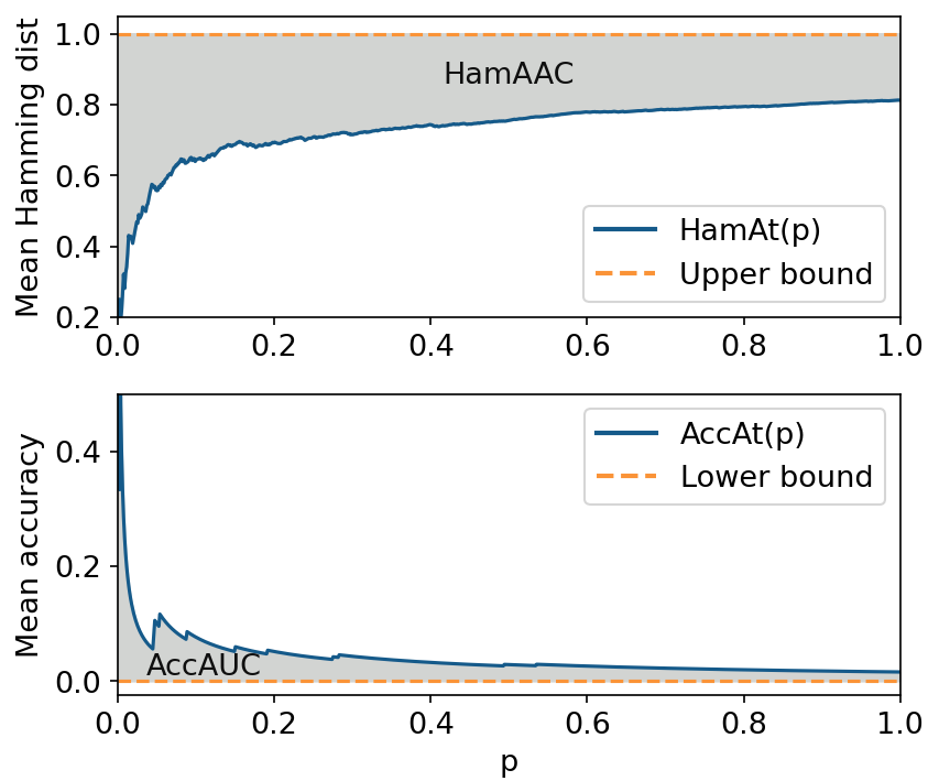
Figure 3: $AccAUC$ and $HamAAC$ computation examples. Acc($p$) denotes the mean accuracy of the top-$p$ fields the adversary is the most confident in. The greater it is, the more accurate the reconstructions are. A peaky and decreasing shape means that the membership inference metric accurately sorts the reconstruction attempts. This is why we seek to maximize its Area Under the Curve ($AccAUC$). Idem for the Area Above the Curve with the Hamming distance ($HamAAC$).

However, common metrics used in the literature do not satisfy these properties. Indeed, existing work such as [9, 84] assess separately the quality of the reconstructions and the membership inference attack. For example, with the regular AUC score computed with the ROC curve, a value of 1.00 is achieved in the two following situations, despite the apparent superiority of the latter: (1) a single perfect reconstruction is ranked highest, trailed by 99 inaccurate reconstructions; and (2) all 100 reconstructions are perfect. This is because AUC score ignores the prevalence of perfect reconstruction, which is necessary to meet the second property we want.

This motivates the introduction of two new metrics that satisfy these properties. Figure 3 demonstrates an example of their computation. We will introduce them briefly, and we refer to the appendix for rigorous definitions and proofs that they satisfy the two desired properties.

Accuracy-AUC and Hamming-AAC

First, we introduce the Accuracy-at-$p$ metric for $p\in[0,1]$ ($AccAt(p)$). It represents the accuracy of the reconstruction within the top-$p$ fields the adversary is the most confident in, i.e. the one with the greatest membership inference metric. Then, we plot $AccAt(p)$ versus $p$. A greater Area Under the Curve ("AUC") means that that the reconstruction are more accurate. This motivates the introduction of the Accuracy-AUC metric.

Similarly, $HamAt(p)$ represents the mean normalized Hamming distance [28] within the top-$p$ fields the adversary is the most confident in. However, we look at the Area Above the Curve ("AAC") because it is a distance and not a similarity. This results in the Hamming-AAC metric. Both the $AccAUC$ and $HamAAC$ metrics take values between 0 and 1, and increase as the quality of the attack improves.

6 Experimental results

This section presents the experimental results of our attack and discusses our main findings. For a comprehensive presentation of our results, please refer to the appendix. Our experiments show that CDMI achieves robust results, allowing for meaningful reconstructions with every task and dataset we evaluated, including numbers, dates, and names up to 8 tokens. Table 3 shows examples of perfect reconstruction.

In our experiments, the maximum value of $AccAt(1.0)$ that we reach is 0.041, meaning that under optimal conditions, the adversary can flawlessly reconstruct 4.1% of the fields. For comparison, under identical conditions, our baseline only recovers 0.77% of the fields. Furthermore, the maximum $AccAt(0.05)$ registered is a promising 22.5%. This indicates that in this scenario, when the adversary employs a membership inference metric to retain the 40 fields they are most confident in (5% of the dataset), they can attain up to 9 perfect reconstructions. This performance far exceeds our baseline’s score at 2.5%, corresponding to just a single field.

Data	Archi	Task	Reconstruction	Len	Occ
SRO	LayoutLM	EE-SPD	restaurant jiawei jiawei house	6	1
SRO	LayoutLM	EE-BIO	guardian health and beauty sdn bhd	8	1
FUN	LayoutLM	EL	m. a. peterson	5	1
FUN	LayoutLM	EE-SPD	r. g. ryan	5	1
SRO	LayoutLM	MLM	lim seng tho hardware trading	6	1
SRO	LayoutLM	MLM	101. 75	3	2
FUN	LayoutLM	MLM	april 13, 1984	4	1
FUN	BROS	MLM	1. 500. 00	6	1
FUN	BROS	MLM	dr. a. w. spears	7	1

Table 3: Examples of perfect reconstructions.

6.1 Performance of the attack

Factors influencing the one-shot variant with LayoutLM

We observe that certain configurations result in significant outcomes. For example, when selecting the checkpoint with the best validation precision from a bimodal MLM trained on FUNSD, we achieve an improvement factor of 1.395. This means that the CDMI reconstructions are approximately 40% more effective than the ones of our baseline (see line 2 in table 5 in the appendix for more details).

However, some models are more vulnerable than others. Figure 4 compares the performance of the one-shot attack for the 8 MLM models we trained with LayoutLM backbone: unimodal or bimodal, Precision or Loss criterion, and FUNSD or SROIE dataset (see lines 1-8 in table 5 for more details). Interestingly, the difference between FUNSD and SROIE datasets is minor, showing that our attack is robust to at least two type of documents. Moreover, we observe that Precision criterion leads to more vulnerable models than Loss criterion. This is not surprising because they are trained for more epochs, so the model had more time to memorize its training data. Finally, we observe that bimodal models are much more vulnerable than unimodal ones, with a mean improvement factor of 1.296 compared to 1.078. This indicates that the visual encoder memorizes information about the training sample, which our attack efficiently extracts. These aspects are discussed further in section 6.2.

For non-MLM tasks, the factors influencing the one-shot attack are different. Indeed, the attack is very efficient on SROIE dataset, with a mean improvement factor of 1.224. However, it obtains poor results on FUNSD, with a mean improvement factor of 1.036, indicating that the attack is not significantly better than the baseline. We explain this result by observing that these models exhibit significantly lower accuracy on FUNSD compared to SROIE, so it is not surprising that the attack can extract less information from them (see columns 6-7, lines 9-24 in table 5 for more details).

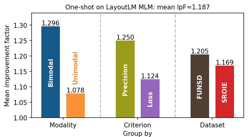
Figure 4: Factors influencing the performance of the one-shot attack on a LayoutLM with MLM task. We attack 8 different models (2 modality, 2 criteria, 2 datasets) with an average improvement factor of $\text{IpF}=1.187$. Among them, the 4 attacks implying a bimodal model are more accurate than those against a unimodal model (IpF of $1.296$ vs. $1.078$). Similarly, the attacks are more accurate with the Precision criterion, and with the FUNSD dataset.

Comparison between the tasks

With LayoutLM backbone, some tasks are easier to attack than others, as outlined in figure 5. MLM task is the most vulnerable, as expected. Indeed, it is designed to reconstruct masked tokens, aligning with the objective of the reconstruction. On the opposite, models trained with EL task exhibit lower validation accuracy compared to EE-BIO and EE-SPADE, which explains their low susceptibility to our attack. Since the model struggles in learning meaningful patterns to solve the task, using its loss as per the CDMI approach makes it less efficient.

However, we observe that for every task and dataset, there exists a configuration yielding an improvement factor of a minimum of $1.10$. This suggests that our reconstruction attack could be generalized to a wider range of fine-tuning tasks, such as document classification and question answering.

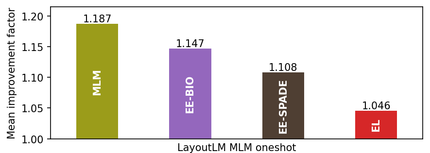
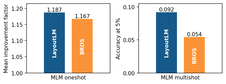
Figure 5: Performance comparison based on the backbone or task. The top graph shows the average performance of the attack with LayoutLM backbone, for the four possible tasks. The bottom graphs compare the average performance of the attack on the MLM models with LayoutLM backbone (in blue) or BROS backbone (in orange), for both the one-shot variant (left) and the multi-shot variant (right).

Comparison between LayoutLM and BROS

As detailed in section 5, we have optimized our attack with the LayoutLM backbone, and then evaluated its transferability to BROS architecture. Thus, it is unsurprising that we obtain stronger results for LayoutLM than BROS. For example, we obtain poor results for most one-shot and multi-shot configurations with non-MLM tasks when using BROS backbone.

However, the outcomes of CDMI for MLM tasks on BROS are highly competitive compared to those on LayoutLM, as outlined in figure 5. For the one-shot variant, there is a minor gap between LayoutLM and BROS backbones, with a mean improvement factor of $1.187$ and $1.167$, respectively. Our best performance for the one-shot variant is even obtained with BROS backbone, with an impressive improvement factor of 1.54. For the multi-shot variant with BROS backbone, 5.4% of the fields are perfectly reconstructed on average within the top-5% fields (Accuracy-at-5%). This is much higher than the accuracy of 1.3% obtained with the baseline, showing that the model memorizes a significant part of its training set.

The successful transferability of our attack to BROS backbone in some settings suggests that it could likely be adapted to other document understanding model architectures.

The multi-shot variant

We observe that many configuration yielding good results with the one-shot variant perform poorly with the multi-shot variant. Thus, in these configurations, even though the model memorizes information about its training data, it is not sufficient to perfectly reconstruct a significant portion of the fields with high confidence.

However, some configurations lead to strong results for both MLM and non-MLM tasks. For example, figure 6 displays a successful attack on a very realistic model trained on EE-SPADE task, which is targeted at epoch 4, when its validation loss is minimal. The adversary perfectly reconstructs 15% of the fields they are most confident in. Moreover, the peaked shapes of $AccAt(p)$ and $HamAt(p)$ indicate that the membership inference metric efficiently sorts the good reconstructions first. As a result, CDMI reconstructions considerably outperform our baseline in all evaluation metrics.

This proves that even non-generative models trained on entity extraction tasks can be successfully attacked.

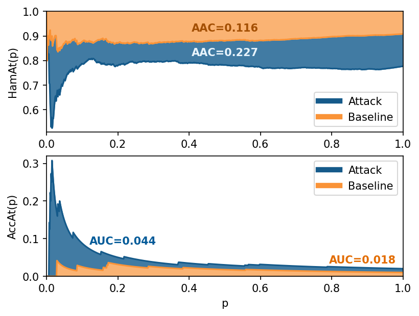
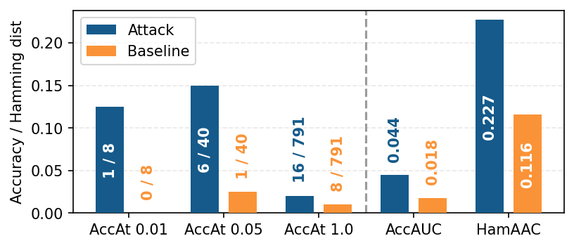
Figure 6: Comparison between the attack and the baseline in a multi-shot setting, with a bimodal model, LayoutLM backbone, EE-SPADE task, SROIE dataset and Loss criterion. On the upper plot, the Hamming-at-$p$ distance is much lower for the attack. On the middle plot, the Accuracy-at-$p$ of the attack is decreasing, so the membership inference metric accurately sorts the most credible reconstructions. On the last plot, the evaluation metrics are higher for the attack: for instance, with $p=0.05$, the attack perfectly reconstructs $6/40=15\%$ of the fields, vs. $1/40=2.5\%$ for the baseline.

6.2 Ablation studies

In this section, we demonstrate that neither overfitting nor data duplication accounts for the performance of our attack. Moreover, we demonstrate that we can extract information memorized by the visual modality, proving that documents should be considered as a distinct data type, susceptible to attacks that can exploit their bimodal nature.

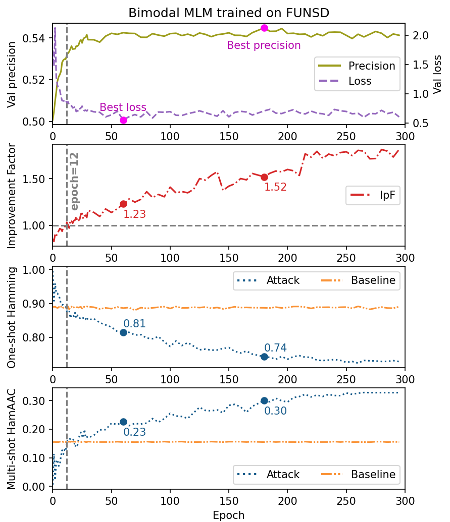
Figure 7: Attacking a bimodal LayoutLM model trained on FUNSD with MLM task and $N_{c}=256$. The first graph plots the validation loss and accuracy, with the best values achieved at epoch 60 and epoch 180, respectively. The two following plots display the performance of the one-shot attack, and the last one shows the performance of the multi-shot attack. In both cases, the attack is more accurate than the baseline from epoch 12, well before the best validation loss.

Overfitting

As detailed in section 2.2, overfitting often favors the memorization of training data, even though it is not a requisite condition [83, 85, 21, 9]. We also observed this phenomenon with CDMI. From the early stages of training, even before the model can overfit, training data are memorized. And the attack performance gradually increases over epochs, even when validation accuracy starts to decrease.

To verify the correlation, we executed the experiment depicted in figure 7. We evaluate the one-shot and multi-shot CDMI attacks on 40% of the fields for one out of 5 model checkpoints between epoch 1 and 300. First, we observe that overfitting is evident, as the best validation loss is achieved much earlier than the best validation precision. However, the attack outperforms the baseline quite early, after just 12 epochs, showing that the model memorizes training data without needing to overfit. Finally, all the performance metrics of our attack increase with the number of training epochs, and persist beyond the epoch with the optimal precision.

This shows that our attack is efficient from the early epochs of training, and that simple regularization techniques are unlikely to be sufficient to ensure the security of the data used to train document understanding models.

Data duplication

Data duplication is known to favor memorization of training data (see section 2.2 and [43]). Certain definitions such as $k$-eidetic memorization [9] even include the number of duplicates. However, defining duplication for document data is not straightforward. In our case, we seek to reconstruct the fields in their context: for example, the reconstruction of "24.8 mm" only becomes useful when it is linked to the form it comes from. Therefore, we deemed that two forms with identical headers but different answers were not duplicates, contrary to shifted or rotated documents.

We did not implement an automatic count of duplication within our datasets; however we manually checked the number of occurrences for a few documents (see "Occ" column in table 3). Even though we observed some duplicates in the SROIE dataset, we did not detect any of them in FUNSD. Thus, we conclude that the good results of our attack is presumably not linked to data duplication. However, further investigating this issue would be a promising topic for future research, as numerous document datasets contain a great number of similar documents (e.g. ID cards, etc.).

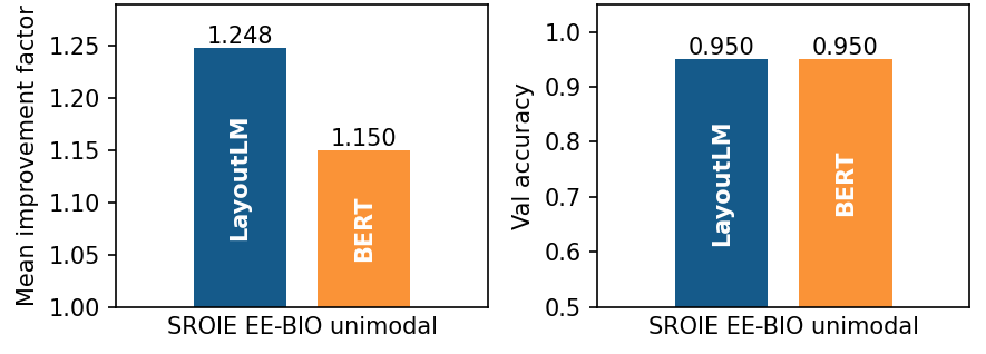
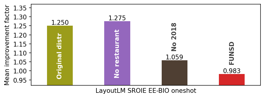
Figure 8: Upper plot: our attack performs better on LayoutLM backbones than BERT. This confirms that layout contributes to memorization, making document models more vulnerable. Lower plot: the performance of attacks using auxiliary public MLM trained on four datasets with increasing distribution shift. Our attack remains feasible if the adversary has access to different yet similar data distribution.

Importance of layout and visual modality

Our attack was designed to efficiently reconstruct data from layout-aware document models. However, it could be possible that it only extracts information from textual content, and would be just as effective on text-only models. We conducted the following experiments to demonstrate that it is not the case, and that both layout and visual modality contribute to memorization.

As shown in the upper plot of figure 8, we trained several models with BERT backbone [13], which does not take the layout into account, and compared them with those using LayoutLM backbone. We specifically used models trained on SROIE with the EE-BIO task, as in this setting, the validation accuracy between BERT and LayoutLM is similar. This means that a difference in memorization cannot be attributed to a difference in accuracy. We observed that the attack is much more successful with LayoutLM, with a mean improvement factor of 1.248 compared to 1.150 with BERT. This proves that layout information contributes to memorization, making the layout-aware models more vulnerable than their textual counterparts.

The significance of visual modality was already discussed in section 6.1. As depicted in figure 4, bimodal models are more susceptible to our attack than unimodal ones. To confirm that the information is memorized within visual modality, we conducted an experiment using bimodal models trained on MLM task with LayoutLM backbone. We obtained a mean improvement factor of 1.296 when attacking these models normally. However, when we deactivated the visual modality by replacing it with Gaussian noise in these models, the mean improvement factor dropped significantly to 1.044. This confirms that our attack extracts information that is memorized within the visual modality.

Robustness to distribution shifts

As explained in section 3, we assume that the adversary knows the target distribution $\mathcal{D}$, and uses it to train an efficient auxiliary public MLM. This hypothesis is plausible given the accessibility of many datasets online, but it gives an advantage to the adversary.

To evaluate its impact, we conducted attacks on SROIE dataset using auxiliary public MLM trained on four datasets with increasing distribution shifts (see figure 8). The first one was trained with the original distribution. For the second one, we removed all restaurant receipts from SROIE, which represents a sub-population of about 10%. We obtained a similar improvement factor, indicating that our attack remains feasible with a minor distribution shift. The third one was trained without any receipt dated 2018 (around 50% of the dataset). This is an important distribution shift because the ‘date’ field is one of those we are attacking. The performance dropped, because the adversary is unable to accurately select relevant candidate tokens. Finally, the last auxiliary model was trained on FUNSD. Here, the distribution shift is too important and the attack is ineffective, yielding an improvement factor close to 1. We conclude that the ability of the adversary to train a well-performing auxiliary model on a nearby distribution is an important assumption for the success of our attack.

7 Conclusion

A pioneer attack

In this paper, we introduce the first reconstruction attack against document understanding models: CDMI (Combinatorial Document Model Inversion). Despite similarities with some attacks against language models, what sets CDMI apart is that it is explicitly designed to handle documents as multimodal data, making it the first to target layout-aware models. We present two variants of the attack: a one-shot version, and a multi-shot version where CDMI is combined with a membership inference attack.

We also establish a meticulous protocol to assess our attack, comparing it with reconstructions that can be made with only public information. We also introduce two new evaluation metrics, Accuracy-AUC and Hamming-AAC, designed to simultaneously evaluate the reconstruction phase and the membership inference phase in the multi-shot variant.

Empirical evidence

We demonstrate that models trained on Key Information Extraction tasks under realistic conditions are vulnerable to reconstruction attacks. Under optimal conditions, the adversary is able to perfectly reconstruct from 4.1% of the fields to 22.5% when combined with a membership inference attack.

We clearly observe that the Masked Language Modelling task is more vulnerable than the Key Information Extraction ones. Moreover, we demonstrate that both layout and visual modality contribute to memorization, making document models more vulnerable than their textual counterparts, and susceptible to specific attack developments.

We show that our attack’s performance is not a consequence of either overfitting or data duplication. It only takes a dozen epochs to memorize training data even without duplication. Thus, further research into alternative defense mechanisms, such as differential privacy, is necessary.

Recommendations

We recommend three mechanisms to make the prerequisites of our attack impossible. First, avoid open-sourcing the weights of models trained on sensitive data. Second, when serving models through an API, hide your model’s confidence score and filter repetitive queries on similar data. Third, avoid sharing anonymized documents, as they can be used for reconstruction attacks.

If these three mechanisms cannot be implemented in a particular situation, we recommend exercising the utmost caution. More advanced reconstruction attacks are likely to be developed in the near future. Our attack method can be used to estimate the privacy risk of a model, and we also advocate for the use of provable privacy-preserving techniques.

We hope our work will alert researchers and practitioners to the privacy risks of document understanding models, and lay the foundation for the development of robust, privacy-preserving architectures.

Appendix

A Training conditions

This section elaborates on aspects discussed in section 5.1.

First, table 4 shows the volumes of the datasets we used. We used two datasets: FUNSD [40] and SROIE [35], which we split into three non-overlapping parts: validation, train-public, and train-private. Column 3 displays the number of documents in each part. Columns 4 and 5 present the total number of fields in each dataset, and the number of fields we selected for our attack, respectively.

Second, the results of our hyperparameter optimization are as follows. For step 1, $N_{c}=128$ offers a satisfactory balance between performance and computational time ($N_{c}=512$ marginally improves the attack accuracy by 2%, at a significant computational cost). For steps 3 and 4, effective results were typically associated with a low temperature, about 0.2–0.4, with a decay rate applied over 3 steps for the PUB-MLM softmax, and no decay for the target one. For step 5, geometric mean exhibited superior results, though the optimal weight varied considerably across configurations (between 0.2 and 0.6). For step 6, the optimal parameter was $p=0.10$, except for some settings where $p=0.12$ proved superior. Finally, we selected $n_{a}=8$ attempts for the multi-shot variant.

Dataset	Partition	# doc	# field	# selected
FUNSD	Valid	50	809	495
FUNSD	Train-PUB	74	1436	911
FUNSD	Train-PRI	75	1296	777
SROIE	Valid	100	400	301
SROIE	Train-PUB	263	1052	796
SROIE	Train-PRI	263	1052	791

Table 4: Number of documents and fields in our partitions.

Backbone	Task	Data	Crit	Modal	Prec	IpF	HamAAC	AccAUC	AccAt 1%	AccAt 5%	AccAt 100%
LayoutLM	MLM	FUN	Prec	UniM	0.545	1.132	0.153	0.020	0.125	0.051	0.009
LayoutLM	MLM	FUN	Prec	BiM	0.545	1.395	0.274	0.061	0.125	0.154	0.027
LayoutLM	MLM	FUN	Loss	UniM	0.543	1.123	0.198	0.021	0.125	0.077	0.010
LayoutLM	MLM	FUN	Loss	BiM	0.543	1.171	0.181	0.034	0.250	0.103	0.013
LayoutLM	MLM	SRO	Prec	UniM	0.540	1.081	0.104	0.036	0.000	0.075	0.020
LayoutLM	MLM	SRO	Prec	BiM	0.538	1.393	0.191	0.070	0.125	0.225	0.032
LayoutLM	MLM	SRO	Loss	UniM	0.534	0.977	0.077	0.017	0.000	0.025	0.010
LayoutLM	MLM	SRO	Loss	BiM	0.534	1.226	0.112	0.031	0.000	0.025	0.021
LayoutLM	EE-BIO	FUN	Prec	UniM	0.762	1.075	0.216	0.016	0.125	0.026	0.008
LayoutLM	EE-BIO	FUN	Prec	BiM	0.746	1.024	0.201	0.004	0.000	0.000	0.004
LayoutLM	EE-BIO	FUN	Loss	UniM	0.718	1.053	0.203	0.008	0.125	0.026	0.004
LayoutLM	EE-BIO	FUN	Loss	BiM	0.702	1.024	0.188	0.003	0.000	0.000	0.001
LayoutLM	EE-BIO	SRO	Prec	UniM	0.960	1.252	0.231	0.026	0.000	0.025	0.019
LayoutLM	EE-BIO	SRO	Prec	BiM	0.967	1.207	0.204	0.010	0.000	0.000	0.010
LayoutLM	EE-BIO	SRO	Loss	UniM	0.940	1.246	0.249	0.023	0.000	0.025	0.018
LayoutLM	EE-BIO	SRO	Loss	BiM	0.955	1.294	0.231	0.014	0.000	0.000	0.013
LayoutLM	EE-SPD	FUN	Prec	UniM	0.760	1.054	0.177	0.005	0.000	0.000	0.004
LayoutLM	EE-SPD	FUN	Prec	BiM	0.760	1.001	0.181	0.008	0.000	0.026	0.004
LayoutLM	EE-SPD	FUN	Loss	UniM	0.469	1.036	0.144	0.012	0.125	0.026	0.004
LayoutLM	EE-SPD	FUN	Loss	BiM	0.623	0.979	0.170	0.007	0.125	0.026	0.001
LayoutLM	EE-SPD	SRO	Prec	UniM	0.952	1.141	0.213	0.019	0.000	0.050	0.010
LayoutLM	EE-SPD	SRO	Prec	BiM	0.935	1.209	0.192	0.008	0.000	0.000	0.009
LayoutLM	EE-SPD	SRO	Loss	UniM	0.856	1.224	0.227	0.044	0.125	0.150	0.020
LayoutLM	EE-SPD	SRO	Loss	BiM	0.880	1.221	0.205	0.009	0.000	0.050	0.005
LayoutLM	EL	FUN	Prec	UniM	0.240	1.164	0.135	0.012	0.000	0.026	0.013
LayoutLM	EL	FUN	Prec	BiM	0.193	0.986	0.059	0.005	0.000	0.026	0.001
LayoutLM	EL	FUN	Loss	UniM	0.093	1.019	0.118	0.006	0.125	0.026	0.001
LayoutLM	EL	FUN	Loss	BiM	0.000	1.015	0.116	0.002	0.000	0.000	0.001
BROS	MLM	FUN	Prec	UniM	0.546	1.243	0.302	0.051	0.250	0.128	0.021
BROS	MLM	FUN	Prec	BiM	0.546	1.540	0.389	0.078	0.250	0.154	0.041
BROS	MLM	FUN	Loss	UniM	0.543	1.170	0.276	0.038	0.125	0.077	0.019
BROS	MLM	FUN	Loss	BiM	0.539	1.246	0.312	0.041	0.125	0.051	0.023
BROS	MLM	SRO	Prec	UniM	0.541	1.028	0.102	0.007	0.125	0.025	0.001
BROS	MLM	SRO	Prec	BiM	0.539	1.092	0.126	0.008	0.000	0.000	0.006
BROS	MLM	SRO	Loss	UniM	0.534	1.017	0.072	0.000	0.000	0.000	0.000
BROS	MLM	SRO	Loss	BiM	0.534	1.001	0.080	0.000	0.000	0.000	0.000

Table 5: Main experimental results. Columns 1-5 show the target’s model training conditions: backbone (LayoutLM, BROS), task (MLM, EE-BIO, EE-SPADE, EL), dataset (FUNSD, SROIE), criterion (Precision, Loss), modality (Unimodal, Bimodal). Column 6 shows its validation accuracy. Columns 7 and 8-12 show the results of the one-shot and multi-shot attacks, respectively.

B Evaluation of the multi-shot variant

Let us detail further $AccAUC$ and $HamAAC$ metrics introduced in section 5.3. For $p\in[0,1]$, let $T(p)$ be the set of field that are ranked top-$p$ by the membership inference metric, and let $Ham$ be the Hamming distance [28]. We define:

$$AccAt(p):=\frac{1}{|T(p)|}\sum_{f\in T(p)}\mathbb{1}(f=\widetilde{f})\ \ \in[0,1]$$ (7)

$$AccAUC:=\int_{p=0}^{1}AccAt(p)\mathop{}\!\mathrm{d}p\ \ \in[0,1]$$ (8)

$$HamAt(p):=\frac{1}{|T(p)|}\sum_{f\in T(p)}Ham(f,\widetilde{f})\ \ \in[0,1]$$ (9)

$$HamAAC:=1-\int_{p=0}^{1}HamAt(p)\mathop{}\!\mathrm{d}p\ \ \in[0,1]$$ (10)

Let us now prove that $HamAAC$ satisfies the two properties of section 5.3; the demonstration is similar for $AccAUC$:

1. Let us fix the values of all $f$ and $\widetilde{f}$. Then, let be two indices $1\leq i<j\leq M$ such that $Ham(f_{i},\widetilde{f_{i}})>Ham(f_{j},\widetilde{f_{j}})$. If we swap $i$ and $j$, this will increase $HamAt(p)$ for $p\in[i/M,j/M[$ leaving the other values unchanged, which will increase the $HamAAC$ score. As a result, every step of a selection sort applied to sort the indices by increasing values of $Ham(f_{i},\widetilde{f_{i}})$ will increase $HamAAC$, proving that the maximum will be achieved at the end of the selection sort.

2. Let $F$ and $\widetilde{F}$ have fixed order, and length $M$, and let $i\in\llbracket 1,M\rrbracket$. Then, if we change the reconstruction $\widetilde{f_{i}}$ into another $\widetilde{f_{i}^{\prime}}$ such that $Ham(f_{i},\widetilde{f_{i}^{\prime}})>Ham(f_{i},\widetilde{f_{i}})$, it is clear that $\forall p\geq i/M$, $HamAt(p)$ increases. As a result, this improvement of $\widetilde{f_{i}}$ increases $HamAAC$ as well.

C Detailed experimental results

Table 5 details our experimental results, using $N_{c}=128$ candidates. We excluded non-MLM tasks with BROS backbone because of their lower results (see section 6.1).

References

- [1] Martín Abadi et al. “Deep Learning with Differential Privacy” In ACM SIGSAC CCS, 2016, pp. 308–318 DOI: 10.1145/2976749.2978318
- [2] D Ackley, G Hinton and T Sejnowski “A learning algorithm for boltzmann machines” In Cognitive Science 9.1, 1985, pp. 147–169
- [3] Nasser Alshammari and Saad Alanazi “The impact of using different annotation schemes on named entity recognition” In Egyptian Informatics Journal 22.3, 2021, pp. 295–302 DOI: 10.1016/j.eij.2020.10.004
- [4] Srikar Appalaraju et al. “DocFormer: End-to-End Transformer for Document Understanding” In IEEE/CVF ICCV, 2021 DOI: 10.48550/arXiv.2106.11539
- [5] Hannah Brown et al. “What Does it Mean for a Language Model to Preserve Privacy?” In ACM FAccT, 2022, pp. 2280–2292 DOI: 10.1145/3531146.3534642
- [6] Paweł Budzianowski and Ivan Vulić “Hello, It’s GPT-2 - How Can I Help You? Towards the Use of Pretrained Language Models for Task-Oriented Dialogue Systems” In NGT, 2019, pp. 15–22 DOI: 10.18653/v1/D19-5602
- [7] Nicholas Carlini et al. “Extracting Training Data from Diffusion Models” In USENIX Security, 2023 DOI: 10.48550/arXiv.2301.13188
- [8] Nicholas Carlini et al. “Quantifying Memorization Across Neural Language Models”, 2022 DOI: 10.48550/arXiv.2202.07646
- [9] Nicholas Carlini et al. “Extracting Training Data from Large Language Models.” In USENIX Security, 2021 DOI: 10.48550/arXiv.2012.07805
- [10] Zhanzhan Cheng et al. “TRIE++: Towards End-to-End Information Extraction from Visually Rich Documents”, 2022 DOI: 10.48550/arXiv.2207.06744
- [11] Andrea Continella et al. “Obfuscation-Resilient Privacy Leak Detection for Mobile Apps Through Differential Analysis” In NDSS, 2017 DOI: 10.14722/ndss.2017.23465
- [12] Sumanth Dathathri et al. “Plug and Play Language Models: A Simple Approach to Controlled Text Generation”, 2019 DOI: 10.48550/arXiv.1912.02164
- [13] Jacob Devlin et al. “BERT: Pre-training of Deep Bidirectional Transformers for Language Understanding” In NAACL, 2019 DOI: 10.18653/v1/N19-1423
- [14] Mohamed Dhouib, Ghassen Bettaieb and Aymen Shabou “DocParser: End-to-end OCR-free Information Extraction from Visually Rich Documents” In ICDAR, 2023 DOI: 10.48550/arXiv.2304.12484
- [15] Josep Domingo-Ferrer, David Sánchez and Alberto Blanco-Justicia “The limits of differential privacy (and its misuse in data release and machine learning)” In CACM, 2021 DOI: 10.1145/3433638
- [16] Cynthia Dwork “A firm foundation for private data analysis” In CACM, 2011 DOI: 10.1145/1866739.1866758
- [17] Cynthia Dwork et al. “Calibrating Noise to Sensitivity in Private Data Analysis” In TCC, 2006 DOI: 10.1007/11681878_14
- [18] Cynthia Dwork and Aaron Roth “The Algorithmic Foundations of Differential Privacy” In FnT-TCS, 2014 DOI: 10.1561/0400000042
- [19] Adel Elmahdy, Huseyin A. and Robert Sim “Privacy Leakage in Text Classification A Data Extraction Approach” In PrivateNLP, 2022 DOI: 10.18653/v1/2022.privatenlp-1.3
- [20] Adel Elmahdy and Ahmed Salem “Deconstructing Classifiers: Towards A Data Reconstruction Attack Against Text Classification Models”, 2023 DOI: 10.48550/arXiv.2306.13789
- [21] Vitaly Feldman “Does learning require memorization? a short tale about a long tail” In ACM SIGACT STOC, 2020, pp. 954–959 DOI: 10.1145/3357713.3384290
- [22] Jessica Ficler and Yoav Goldberg “Controlling Linguistic Style Aspects in Neural Language Generation” In Style-Var, 2017, pp. 94–104 DOI: 10.18653/v1/W17-4912
- [23] Matt Fredrikson, Somesh Jha and Thomas Ristenpart “Model Inversion Attacks that Exploit Confidence Information and Basic Countermeasures” In ACM SIGSAC CCS, 2015, pp. 1322–1333 DOI: 10.1145/2810103.2813677
- [24] Matthew Fredrikson et al. “Privacy in Pharmacogenetics: An End-to-End Case Study of Personalized Warfarin Dosing” In USENIX Security, 2014
- [25] Łukasz Garncarek et al. “LAMBERT: Layout-Aware Language Modeling for Information Extraction” In ICDAR, 2021 DOI: 10.48550/arXiv.2002.08087
- [26] Kartik Goyal, Chris Dyer and Taylor Berg-Kirkpatrick “Exposing the Implicit Energy Networks behind Masked Language Models via Metropolis–Hastings” In ICLR, 2022 DOI: 10.48550/arXiv.2106.02736
- [27] He Guo et al. “EATEN: Entity-Aware Attention for Single Shot Visual Text Extraction” In ICDAR, 2019 DOI: 10.1109/ICDAR.2019.00049
- [28] R.. Hamming “Error detecting and error correcting codes” In The Bell System Technical Journal 29.2, 1950, pp. 147–160 DOI: 10.1002/j.1538-7305.1950.tb00463.x
- [29] Adam W. Harley, Alex Ufkes and Konstantinos G. Derpanis “Evaluation of Deep Convolutional Nets for Document Image Classification and Retrieval” In ICDAR, 2015, pp. 991–995 DOI: 10.1109/ICDAR.2015.7333910
- [30] Kaiming He et al. “Mask R-CNN” In IEEE ICCV, 2017, pp. 2980–2988 DOI: 10.1109/ICCV.2017.322
- [31] Ari Holtzman et al. “The Curious Case of Neural Text Degeneration” In ICLR, 2019 DOI: 10.48550/arXiv.1904.09751
- [32] Teakgyu Hong et al. “BROS: A Pre-trained Language Model Focusing on Text and Layout for Better Key Information Extraction from Documents” In AAAI, 2021 DOI: 10.1609/aaai.v36i10.21322
- [33] Hongsheng Hu et al. “Membership Inference Attacks on Machine Learning: A Survey” In ACM Surveys, 2022 DOI: 10.1145/3523273
- [34] Yupan Huang et al. “LayoutLMv3: Pre-training for Document AI with Unified Text and Image Masking” In ACM Multimedia, 2022, pp. 4083–4091 DOI: 10.1145/3503161.3548112
- [35] Zheng Huang et al. “ICDAR2019 Competition on Scanned Receipt OCR and Information Extraction” In ICDAR, 2019, pp. 1516–1520 DOI: 10.1109/ICDAR.2019.00244
- [36] Wonseok Hwang et al. “Spatial Dependency Parsing for Semi-Structured Document Information Extraction” In ACL-IJCNLP, 2021 DOI: 10.18653/v1/2021.findings-acl.28
- [37] Shotaro Ishihara “Training Data Extraction From Pre-trained Language Models: A Survey”, 2023 DOI: 10.48550/arXiv.2305.16157
- [38] Eric Jang, Shixiang Gu and Ben Poole “Categorical Reparameterization with Gumbel-Softmax”, 2017 DOI: 10.48550/arXiv.1611.01144
- [39] Matthew A. Jaro “Advances in Record-Linkage Methodology as Applied to Matching the 1985 Census of Tampa, Florida” In Journal of the ASA, 1989 DOI: 10.1080/01621459.1989.10478785
- [40] Guillaume Jaume, Hazim Kemal Ekenel and Jean-Philippe Thiran “FUNSD: A Dataset for Form Understanding in Noisy Scanned Documents” In ICDAR, 2019 DOI: 10.1109/ICDARW.2019.10029
- [41] F. Jelinek et al. “Perplexity—a measure of the difficulty of speech recognition tasks” In The Journal of the Acoustical Society of America 62.S1, 1977, pp. S63–S63 DOI: 10.1121/1.2016299
- [42] Mostafa Kahla et al. “Label-Only Model Inversion Attacks via Boundary Repulsion” In IEEE/CVF CVPR, 2022, pp. 15025–15033 DOI: 10.1109/CVPR52688.2022.01462
- [43] Nikhil Kandpal, Eric Wallace and Colin Raffel “Deduplicating Training Data Mitigates Privacy Risks in Language Models” In ICML 162, 2022, pp. 10697–10707 DOI: 10.48550/arXiv.2202.06539
- [44] Mahdi Khosravy et al. “Model Inversion Attack by Integration of Deep Generative Models: Privacy-Sensitive Face Generation From a Face Recognition System” In IEEE TIFS, 2022 DOI: 10.1109/TIFS.2022.3140687
- [45] Geewook Kim et al. “OCR-Free Document Understanding Transformer” In ECCV, 2022 DOI: 10.48550/arXiv.2111.15664
- [46] Jooyoung Lee et al. “Do Language Models Plagiarize?” In ACM WWW, 2022, pp. 3637–3647 DOI: 10.1145/3543507.3583199
- [47] Eric Lehman et al. “Does BERT Pretrained on Clinical Notes Reveal Sensitive Data?” In NAACL, 2021 DOI: 10.18653/v1/2021.naacl-main.73
- [48] Vladimir Iosifovich Levenshtein “Binary codes capable of correcting deletions, insertions and reversals” In Soviet Physics Doklady 10, 1966, pp. 707–710
- [49] D. Lewis et al. “Building a test collection for complex document information processing” In ACM SIGIR, 2006 DOI: 10.1145/1148170.1148307
- [50] Nils Lukas et al. “Analyzing Leakage of Personally Identifiable Information in Language Models” In IEEE S&P, 2023 DOI: 10.1109/SP46215.2023.10179300
- [51] Chuwei Luo et al. “GeoLayoutLM: Geometric Pre-training for Visual Information Extraction” In IEEE/CVF CVPR, 2023 DOI: 10.48550/arXiv.2304.10759
- [52] Saeed Mahloujifar et al. “Membership Inference on Word Embedding and Beyond”, 2021 DOI: 10.48550/arXiv.2106.11384
- [53] Minesh Mathew, Dimosthenis Karatzas and C.. Jawahar “DocVQA: A Dataset for VQA on Document Images” In IEEE/CVF WACV, 2021 DOI: 10.48550/arXiv.2007.00398
- [54] Casey Meehan, Khalil Mrini and Kamalika Chaudhuri “Sentence-level Privacy for Document Embeddings” In Annual Meeting of the ACL, 2022 DOI: 10.18653/v1/2022.acl-long.238
- [55] Fatemehsadat Mireshghallah et al. “Quantifying Privacy Risks of Masked Language Models Using Membership Inference Attacks” In ACL-EMNLP, 2022 DOI: 10.18653/v1/2022.emnlp-main.570
- [56] Fatemehsadat Mireshghallah et al. “Privacy Regularization: Joint Privacy-Utility Optimization in LanguageModels” In NAACL, 2021 DOI: 10.18653/v1/2021.naacl-main.298
- [57] Giannis Nikolentzos, Antoine Tixier and Michalis Vazirgiannis “Message Passing Attention Networks for Document Understanding” In AAAI, 2020 DOI: 10.1609/aaai.v34i05.6376
- [58] Iyiola E. Olatunji, Wolfgang Nejdl and Megha Khosla “Membership Inference Attack on Graph Neural Networks” In IEEE TPS-ISA, 2021 DOI: 10.1109/TPSISA52974.2021.00002
- [59] Rahil Parikh, Christophe Dupuy and Rahul Gupta “Canary Extraction in Natural Language Understanding Models” In Annual Meeting of the ACL 2, 2022, pp. 552–560 DOI: 10.18653/v1/2022.acl-short.61
- [60] Seunghyun Park et al. “CORD: A consolidated receipt dataset for post-OCR parsing” In Document Intelligence Workshop NeurIPS, 2019 URL: https://github.com/clovaai/cord
- [61] Ethan Perez et al. “Red Teaming Language Models with Language Models” In EMNLP, 2022 DOI: 10.18653/v1/2022.emnlp-main.225
- [62] Rafał Powalski et al. “Going Full-TILT Boogie on Document Understanding with Text-Image-Layout Transformer” In ICDAR, 2021 DOI: 10.1007/978-3-030-86331-9_47
- [63] Colin Raffel et al. “Exploring the Limits of Transfer Learning with a Unified Text-to-Text Transformer” In JMLR, 2020 URL: http://jmlr.org/papers/v21/20-074.html
- [64] Nils Reimers and Iryna Gurevych “Sentence-BERT: Sentence Embeddings using Siamese BERT-Networks” In ACL-EMNLP-IJCNLP, 2019 DOI: 10.18653/v1/D19-1410
- [65] Jingjing Ren et al. “ReCon: Revealing and Controlling PII Leaks in Mobile Network Traffic” In ACM MobiSys, 2016 DOI: 10.1145/2906388.2906392
- [66] Shahbaz Rezaei, Zubair Shafiq and Xin Liu “Accuracy-Privacy Trade-off in Deep Ensemble: A Membership Inference Perspective” In IEEE S&P, 2023, pp. 364–381 DOI: 10.1109/SP46215.2023.10179463
- [67] Ahmed Salem et al. “Let the Privacy Games Begin! A Unified Treatment of Data Inference Privacy in Machine Learning” In IEEE S&P, 2023 DOI: 10.1109/SP46215.2023.10179281
- [68] Hanyin Shao et al. “Quantifying Association Capabilities of Large Language Models and Its Implications on Privacy Leakage”, 2023 DOI: 10.48550/arXiv.2305.12707
- [69] Reza Shokri et al. “Membership Inference Attacks against Machine Learning Models” In IEEE S&P, 2017 DOI: 10.1109/SP.2017.41
- [70] Congzheng Song and Ananth Raghunathan “Information Leakage in Embedding Models” In ACM SIGSAC CCS, 2020, pp. 377–390 DOI: 10.1145/3372297.3417270
- [71] Nishant Subramani et al. “A Survey of Deep Learning Approaches for OCR and Document Understanding”, 2021 DOI: 10.48550/arXiv.2011.13534
- [72] Florian Tramèr, Gautam Kamath and Nicholas Carlini “Considerations for Differentially Private Learning with Large-Scale Public Pretraining”, 2022 DOI: 10.48550/arXiv.2212.06470
- [73] Thomas Vakili et al. “Downstream Task Performance of BERT Models Pre-Trained Using Automatically De-Identified Clinical Data” In LREC, 2022 URL: https://aclanthology.org/2022.lrec-1.451
- [74] Ashish Vaswani et al. “Attention Is All You Need” In NeurIPS, 2017 DOI: 10.48550/arXiv.1706.03762
- [75] Alex Wang and Kyunghyun Cho “BERT has a Mouth, and It Must Speak: BERT as a Markov Random Field Language Model” In ACL W19-23, 2019, pp. 30–36 DOI: 10.18653/v1/W19-2304
- [76] Kuan-Chieh Wang et al. “Variational Model Inversion Attacks” In NeurIPS 34, 2022 DOI: 10.48550/arXiv.2201.10787
- [77] Wenjin Wang et al. “Layout and Task Aware Instruction Prompt for Zero-shot Document Image Question Answering”, 2023 DOI: 10.48550/arXiv.2306.00526
- [78] William E. Winkler “String Comparator Metrics and Enhanced Decision Rules in the Fellegi-Sunter Model of Record Linkage” In Proceedings of the Section on Survey Research Methods, 1990, pp. 354–359
- [79] Xi Wu et al. “A Methodology for Formalizing Model-Inversion Attacks” In IEEE CSF, 2016, pp. 355–370 DOI: 10.1109/CSF.2016.32
- [80] Yang Xu et al. “LayoutLMv2: Multi-modal Pre-training for Visually-rich Document Understanding” In ACL-IJCNLP, 2021 DOI: 10.18653/v1/2021.acl-long.201
- [81] Yiheng Xu et al. “LayoutLM: Pre-training of Text and Layout for Document Image Understanding” In ACM SIGKDD, 2019 DOI: 10.1145/3394486.3403172
- [82] Jingfeng Yang et al. “Harnessing the Power of LLMs in Practice: A Survey on ChatGPT and Beyond”, 2023 DOI: 10.48550/arXiv.2304.13712
- [83] Samuel Yeom et al. “Privacy Risk in Machine Learning: Analyzing the Connection to Overfitting” In IEEE CSF, 2018, pp. 268–282 DOI: 10.1109/CSF.2018.00027
- [84] Weichen Yu et al. “Bag of Tricks for Training Data Extraction from Language Models” In ICML, 2023 DOI: 10.48550/arXiv.2302.04460
- [85] Chiyuan Zhang et al. “Understanding deep learning (still) requires rethinking generalization” In CACM 64, 2021 DOI: 10.1145/3446776
- [86] Ruisi Zhang, Seira Hidano and Farinaz Koushanfar “Text Revealer: Private Text Reconstruction via Model Inversion Attacks against Transformers”, 2022 DOI: 10.48550/arXiv.2209.10505
- [87] Yuheng Zhang et al. “The Secret Revealer: Generative Model-Inversion Attacks Against Deep Neural Networks” In IEEE/CVF CVPR, 2020 DOI: 10.1109/CVPR42600.2020.00033
- [88] Zhikun Zhang et al. “Inference Attacks Against Graph Neural Networks” In USENIX Security, 2022 DOI: 10.48550/arXiv.2110.02631