tcb@breakable

Enabling Decision-Making with the Modified Causal Forest: Policy Trees for Treatment Assignment

Abstract

1 Introduction

Policymakers are keen to gain insights into policy impacts, aiming to facilitate future applications. Therefore, current econometrics research is dedicated to developing methods that accurately estimate policy effects, specifically focusing on understanding relevant heterogeneity across sub-populations. However, it is important to distinguish between estimating heterogeneity and providing guidance on the design of treatment assignment mechanisms. The latter pertains to the policy learning research area, which effectively uses information from randomised or observational studies to assign individuals to future treatments.

The seminal work of Manski (2004) pioneered the literature on policy learning, then further developed by Kitagawa and Tetenov (2018); Mbakop and Tabord-Meehan (2021); Athey and Wager (2021); Kitagawa and Tetenov (2021) and Zhou et al. (2023), among others. Specifically, Kitagawa and Tetenov (2018) introduce a policy learner that attains the $\sqrt{N}$ convergence rates in settings with a binary treatment and known propensity scores. Athey and Wager (2021) propose a policy learner that achieves the same convergence rate even without known propensity scores, making it well suited for observational studies. Finally, Zhou et al. (2023) propose the Cross-fitted Augmented Inverse Propensity Weighted Learning (CAIPWL) policy learner, which achieves optimal convergence rates in multi-action settings with unknown propensity scores.

This work presents the mcf Policy Tree as implemented in the mcf package. The policy learner is based on the algorithm proposed by Zhou et al. (2023) but introduces three key modifications: policy scores calculation, implementation of constraints, and different handling of categorical and continuous variables. First, the consistent and asymptotically normally distributed policy scores (or potential outcomes) are computed by the mcf to calculate individualised average treatment effects (IATEs)(Lechner and Mareckova; 2024). They differ from the doubly-robust scores used in the original algorithm since the mcf splitting criterion differs. In particular, the mcf algorithm minimises the estimation errors of the conditional mean responses of the treatments and the covariance of these errors while also taking into account propensity score heterogeneity to reduce selection bias. Additionally, the IATEs differ from doubly robust scores since they depend only on the features and not the outcome and treatment. The second modification concerns the implementation of constraints. They are integrated as treatment-specific cost values in terms of the outcome, which are then subtracted from the policy scores. This also applies to constraints that are only indirectly related to costs, such as constraints on treatment shares. Finally, the mcf Policy Tree differs from existing methods in the literature in handling categorical and continuous features. Traditional approaches in the literature often rely on one-hot encoding for categorical features, which may lead to rather extreme leaves with many different values when building shallow trees due to splitting one category against the remaining ones. In contrast, the mcf Policy Tree employs a distinct procedure that allows several categories on both sides of a split. For a detailed explanation of this approach, refer to Chapter 9.2.4 in Hastie, Tibshirani and Friedman (2009). Beyond this functionality, the mcf algorithm provides flexibility for handling continuous and categorical, unordered features with many possible values by allowing users to specify an approximation parameter. This parameter determines the number of potential splitting points, offering finer granularity compared to the global approximation parameter implemented in Zhou et al. (2023).

This paper contributes to the literature in various ways. First, we demonstrate the application of the Policy Tree algorithm across diverse fields, including medicine, epidemiology, and business, within both randomised and observational research settings. Second, this work provides new empirical results on causal effect heterogeneity and policy learning. In that respect, we evaluate well-known and used data in the respective scientific fields. Third, our results take cost-related constraints for decision-making into account. Fourth, all replication materials, including data and programming codes, can be accessed on Github. To run these codes, the open-source Python package mcf provides the classes ModifiedCausalForest() for estimation and OptimalPolicy() for decision-making.

In the remainder of this paper, Section 2 introduces the framework for identification and estimation and package functionalities. Section 3 shows the setups and findings of the empirical studies. Finally, Section 4 discusses computational facets and concludes.

2 Framework

The mcf package is a forest-based causal machine learning algorithm that produces consistent and asymptotically normal treatment effect estimates for various levels of granularity in randomised control trials and selection-on-observable settings. The latter imposes several assumptions to identify the causal effects, namely ignorability, overlap, the stable unit treatment value assumption, and exogeneity of features; see Imbens and Wooldridge (2009) for more details on these identifying assumptions. The estimands of interests identify the causal effect at different aggregation levels, in particular, the average potential outcomes, the average treatment effect, and conditional average effects like IATEs and grouped aggregates of these effects. The IATEs are the average effects for the most granular sub-groups, identified by specific realisations of the available exogenous features. The evaluation of the IATEs makes it possible to detect potential heterogeneous effects across sub-groups of the population. If heterogeneity is observed, certain individuals may either benefit or not from a particular treatment. This is a crucial starting point for a policy learning analysis, indicating the potential for refining the treatment assignment mechanism and informing policy recommendations.

To address this, we introduce the OptimalPolicy() class of the mcf, which explores the space of all available trees and chooses the optimal one. The optimal tree maximises the value function (or welfare), computed as the sum of the individual policy scores, such as potential outcomes or IATEs, by assigning all observations in a terminal leaf node to a single treatment. For a fixed depth, the tree algorithm implements an exhaustive and recursive search across all pre-specified variables and values. It performs the splits when the policy scores within the leaves (or subsets) are maximised under a specific treatment.

Algorithm 1 illustrates, in a simplified way, how the tree-search algorithm works. To introduce it, we can assume the following notation: For $i$ observations, ${X_{i}}$ represents the features, specifically, $p_{1}$ is the number of ordered features, $p_{2}$ is the number of unordered features, $j\in\{0,\ldots,D\}$ is the treatments space, $\hat{\Theta}_{i}$ is the vector (or matrix) of policy scores for each observation $i$, $\hat{\Theta}_{i}(j)$ is the potential outcome for each observation for each treatment $j$, and $L$ is an integer indicating the depth of the tree plus one.

Algorithm 1 Policy Tree

1:Input: $\{(X_{i},\hat{\Theta}_{i}(j))\}_{i=1}^{n}$, $L$

2:if $L=1$ then

3:     Return $(\max_{j\in\{1,\ldots,d\}}\sum_{i}\hat{\Theta}_{i}(j),\operatorname{argmax}_{j\in\{1,\ldots,d\}}\sum_{i}\hat{\Theta}_{i}(j))$

4:else

5:     Initialise reward $\mathcal{R}\leftarrow-\infty$, and empty tree $\mathcal{T}\leftarrow\emptyset$ for all $m=1,\ldots,p_{1}+p_{2}$

6:     for $m\leftarrow 1,2,\ldots,p_{1}+p_{2}$ do

7:         for sorted values of ordered or unique categories of continuous m-th features do

8:              $\text{reward\_left},\text{tree\_left}\leftarrow\text{Tree-Search}(set_{L},L-1)$

9:              $\text{reward\_right},\text{tree\_right}\leftarrow\text{Tree-Search}(set_{T},L-1)$

10:              if $\text{reward\_left}+\text{reward\_right}>\mathcal{R}$ then

11:                  $\mathcal{R}\leftarrow\text{reward\_left}+\text{reward\_right}$

12:                  $\mathcal{T}\leftarrow\text{Tree-search}(m,\text{splitting value},\text{tree\_left},\text{tree\_right})$

13:              end if

14:         end for

15:     end for

16:     Return $(\mathcal{R},\mathcal{T})$

17:end if

Besides the Policy Tree, the OptimalPolicy() class provides a best-score method to create an assignment rule. This method simply assigns units to the treatment with the highest estimated potential outcome. Although computationally cheap, this best-score method lacks clear interpretability for the allocation rules, which may make it difficult for policymakers to adopt it.

3 Empirical Studies

The mcf package offers empirical researchers dual valuable functionalities: the possibility of conducting heterogeneity analyses, as shown in Bodory, Busshoff and Lechner (2022), and refining the decision-making process by optimising treatment allocation rules. This section studies three real-world applications from different scientific fields based on distinct research settings. In these empirical tasks, we first perform an effect heterogeneity evaluation calling the ModifiedCausalForest() class of the mcf algorithm. We then use the potential outcomes estimated by the mcf to optimise the treatment allocations generated by the Policy Trees using the mcf’s OptimialPolicy() class. The samples from all three studies are split using the same approach. Specifically, 40% of the data is allocated for training the mcf, and another 40% for estimating the effects and training the policy learning algorithm. Finally, the remaining 20% of the data are reserved for predicting out-of-sample policy rules and welfare. This allocation helps to estimate the treatment effect effectively and to mitigate the risk of overfitting, particularly for deeper trees.

3.1 Study 1: Oregon Health Insurance Experiment

In 2008, Oregon initiated a lottery with limited spots to provide low-income individuals access to its Medicaid program. This lottery offers an opportunity to examine the impact of expanding access to public health insurance within a randomised controlled setting. Researchers analysed various outcomes over two years following the experiment, including healthcare utilisation, financial strain, health status, labour market outcomes, and political participation. Extensive studies have been conducted by Finkelstein et al. (2012); Baicker et al. (2013); Finkelstein et al. (2016); Baicker et al. (2017); Carcillo and Grubb (2006); Baicker and Finkelstein (2018); Finkelstein et al. (2019), and Baicker, Finkelstein, Song and Taubman (2014), among others. Overall findings suggest that access to Medicaid leads to an increase in healthcare utilisation and a decrease in financial strain and depression, albeit without statistically significant improvements in physical health or labour market outcomes. This analysis follows Finkelstein et al. (2012) and specifically focuses on the impact of being selected in the lottery on primary care visits during the first year post-selection. We rely on survey data collected within the experimental setting, given that the hospital records are not publicly available. The end-line survey, conducted after 12 months, was completed by 23,777 individuals. The outcome is measured by a binary variable indicating if primary care has been utilised during the year. Among the several outcomes available (e.g. emergency room usage or drug prescription), we choose primary care utilisation because of its importance from a policy perspective. Indeed, primary care visits may lead to preventive care for more serious diseases and, consequently, prevention of more expensive medical care.

After dropping observations with missing values, the size of our dataset is 23,527 observations, with 50% of the individuals with Medicaid health insurance. As in Finkelstein et al. (2012), our intention-to-treat specification incorporates additional features, such as socio-demographic factors, which are valuable for exploring heterogeneity and informing policy, even though they are not essential for identifying causal effects. On the contrary, although assignment to the lottery is random, all family members of randomly selected individuals can apply for Medicaid. Therefore, the probability of receiving treatment depends on the number of family members, which we include as a control variable. Table 5.1 in the Appendix describes the 11 variables used for data analysis.

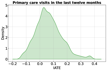
Figure 1: Distribution of IATE

Note: Mean (average standard error) of the IATEs: 0.07 (0.1).

We evaluate the distribution of the IATEs to detect potential effect heterogeneity. Figure 1 displays a density plot of the IATEs, ranging from -0.13 to 0.37, with a mean value of 0.07 and an average standard error of 0.1. The variation in the effects justifies our following analysis for decision-making, aiming at expanding the number of primary care visits by optimising the treatment allocation process.

Table 1 provides details on welfare, measured as utilisation of primary care visits and allocation shares of individuals for various policies. We compare the results of the Policy Trees with our two baseline policies, namely the observed and random treatment allocations. In this study, we examine both unconstrained and constrained Policy Trees. Given the lack of specific cost information for Medicaid insurance, we assume that only approximately half of the population (as in the empirical data) can be covered by this health insurance. The algorithm enforces constraints by finding a cost value to subtract from the policy score. It adjusts the treatment costs to ensure that the allocation of observations to treatments does not exceed the maximum treatment shares. We build our constrained Policy Trees by specifying either the depth of a first optimal tree (Constrained optimal Policy Tree) or, optionally, specifying, in addition, the depth of a second optimal policy tree (Constrained sequentially optimal Policy tree). In the latter case, the second tree is built within the strata obtained from the leaves of the first tree. The final Policy Tree will not be optimal. However, its performance in terms of welfare is comparable to that of an optimal tree with the same depth, with the advantage of reduced computational time.

Policy Welfare (%) Treatment shares (%) Primary care visits Medicaid no Medicaid yes Observed 51.70 49.98 50.02 Random 51.45 50.16 49.84 Unconstrained optimal Policy Tree     Depth-2 54.97 0 100     Depth-3 54.97 0 100 Constrained optimal Policy Tree     Depth-2 52.88 53.56 46.44     Depth-3 53.48 51.75 48.25     Depth-4 53.51 52.18 47.82 Constrained sequentially optimal Policy Trees     Depth-2+1 52.68 57,06 42,93     Depth-3+1 53.54 50.30 49.69 Note: The table shows empirically observed, randomly assigned, and optimal treatment allocations of individuals. The optimal policy trees are unconstrained and constrained. The final constrained trees add a sequential optimal sub-tree (+1). The constraint is implemented as a limit imposed on the treatment shares, as observed within the empirical dataset. The outcome represents primary care visits. The treatment is being extracted from the lottery, which allows one to apply for Medicaid, the public health insurance programme.

Table 1: Treatment allocations Oregon Health Insurance Experiment

In Table 1, all the Policy Trees report an increase in welfare with respect to the baseline policies. The unconstrained Policy Trees achieve the highest welfare, increasing the probability of primary care visits from 51.70% to 54.98%. They allocate almost all individuals to the treatment, which can be interpreted as access to Medicaid insurance for nearly everyone. Compared to the unconstrained Policy Trees, those with the capacity constraint always report a small decrease in the probability of primary care visits, allocating a significantly lower proportion of individuals to the treatment. Constrained optimal Policy Trees and Constrained sequentially optimal Policy Trees, with a last sequential optimal sub-tree of the same depth, show comparable and stable results in terms of welfare achieved. From a computational point of view, such findings may be relevant for large datasets since Policy Trees with the last sequential optimal layers reduce computation time by performing similarly well.

Figure 2 presents the allocation rules of a constrained optimal Policy Tree with a depth of 2. Notably, even at this relatively shallow depth, the Policy Tree demonstrates improvements in welfare compared to the observed allocations and the simplest allocation rules. Individuals with age between 37 and 51 years old (38% of the sample) are assigned to Medicaid. Additionally, individuals older than 51 living in metropolitan areas, constituting 9% of our sample, are also allocated to the program. Conversely, individuals younger than 36 and older than 51 who do not live in metropolitan areas are excluded from the program. For reference, note that the age ranges from 20 to 63.

Figure 2: Allocation rule for a constrained optimal Policy Tree of depth-2

Note: The policy tree shows the shares of individuals allocated to each treatment. The splitting variables of the tree are age and an indicator variable for living in a metropolitan area (MSA). The final leaves of the trees indicate the treatments and corresponding shares of allocated individuals. The treatment used in the analysis is the indicator for being assigned to the lottery, which consequently gives access to Medicaid. For representation reasons, the tree reports: No-MA: No access to Medicaid (not extracted for the lottery), MA: Access to Medicaid (extracted for the lottery).

3.2 Study 2: Right Heart Catheterization

In a seminal study, Connors, Speroff, Dawson, Thomas, Harrell, Wagner, Desbiens, Goldman, Wu, Califf et al. (1996) investigated the impact of Right Heart Catheterization (RHC) on various outcomes, including subsequent survival, healthcare costs, intensity of care, and length of hospital stay. Their findings revealed a positive association between RHC and mortality, as well as increased costs and prolonged length of stay. This conclusion was corroborated by subsequent research utilising different estimation methods, such as those employed by Knaus et al. (1995), Ramsahai et al. (2011), Keele and Small (2018), and Keele and Small (2021). In accordance with previous research, we also use the dataset originally collected from the SUPPORT prospective cohort study (Study to Understand Prognoses and Preferences for Outcomes and Risks of Treatments) as in Connors et al. (1996). This dataset includes 5,735 observations on ill and hospitalised individuals between 1989 and 1994 in five medical centres in the US. 38% of the patients received the surgery. Bodory et al. (2022) utilise the same information to provide new results on effect heterogeneity by exploring the functionalities of the mcf package.

In this empirical application, we focus on finding an optimal allocation of RHC to patients to increase their probability of survival six months after the medical surgery. Previous work exploits expert opinion to identify eight features as relevant confounding factors (Ramsahai et al.; 2011). These features include an index of activities of daily living two weeks before admission, age, the acute physiology and chronic health evaluation score (APACHE III), the Glasgow coma score, mean blood pressure, the probability of surviving two months (based on model estimations), an indicator for do not resuscitation status on the first day, and information on nine primary disease categories. Recognising the significance of these factors, we employ them as features in the Policy Tree to obtain assignment rules for decision-making. Age and mean blood pressure are continuous variables, and we allow the tree algorithm to automatically determine the optimal split points based on the default number of evaluation points in the mcf package.

Our analysis starts by estimating the policy scores and IATEs. Additionally to the high-priority factors, we include potential confounding features (e.g. information on having cancer, possessing health insurance, etc.) to achieve identification through a selection-on-observable approach. Table 5.1 of the Appendix comprehensively describes all 55 confounders.

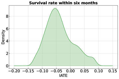
Figure 3: Distribution of IATE

Note: Mean (average standard error) of the IATEs: -0.04 (0.06).

Figure 3 displays the density function of the IATEs, the most granular treatment effects. While slightly right-skewed, the distribution shows positive and negative treatment effects, ranging from -0.12 to 0.08, and an average standard error of 0.06. This result underscores the (rather moderate) heterogeneous response to the surgery, indicating that while some individuals benefit from the intervention, others do not. Such heterogeneity emphasises the importance of conducting a treatment allocation analysis to investigate potential improvements in the allocations of individuals.

Table 2 shows that simple allocation schemes may improve the overall survival rate while decreasing the number of surgeries at the same time. Again, the first two rows of Table 2 present results using the empirically observed and random assignment of individuals to treatments, which are used as baseline comparison policies. The remaining rows show the results of Policy Trees aiming to optimise the treatment allocation and increase the survival rate. Given the relatively small sample size, this study focuses on optimal trees of depths two and three, alongside Policy Trees with depths 3 and 4, including a final sequential optimal sub-tree (+1).

Policy Welfare (%) Treatment shares (%) Survival rate no RHC yes RHC Observed 68.23 60.51 39.49 Random 67.88 59.00 40.99 Unconstrained optimal Policy Tree     Depth-2 69.99 80.78 19.21     Depth-3 69.95 82.73 17.27 Unconstrained sequentially optimal Policy Trees     Depth-2+1 69.98 82.88 17.11     Depth-3+1 69.97 83.78 16.22 Note: The table displays empirically observed, randomly assigned, and optimised treatment allocations as policies, where the final two Policy Trees add a second optimal sub-tree (+1).

Table 2: Treatment allocations Right Heart Catheterization

Table 2 first reveals that the observed treatment allocation outperforms a random treatment assignment in terms of the survival rate (68.23% vs. 67.88%). Considering the performance of the Policy Trees, the findings suggest treatment allocations that could further increase the average survival rate within six months after the intervention up to 69.99% while significantly diminishing the number of individuals receiving surgery by more than 50%. The maximum welfare gain, among the Policy Trees estimated, is already achieved with a Policy Tree of depth two. Deeper trees do not lead to a relevant increase in the survival rate. However, they reduce the share of individuals undergoing an operation. For example, compared to the depth-2 tree, the depth-3+1 tree indicates a reduction in survival rate by only 0.02 percentage points (69.99% vs. 69.97%) but decreases the share of patients having surgery by nearly three percentage points (19.21% vs. 16.22%).

Since the maximum welfare gain is already attained with a depth-2 tree, Figure 4 displays the decision rules established by this tree, which is also the most straightforward to interpret. The Policy Tree performs the first split on age, while the second splitting variable is the estimated probability of surviving within two months, measured before the surgery. The decision tree allocates individuals to surgery with an age below 65 years and a survival probability below 48%, as well as with an age above 65 years and a survival probability below 40%. Note that tables representing all Policy Tree rules used are available in the Appendix.

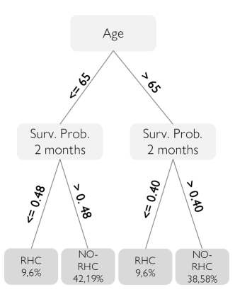
Figure 4: Allocation rule for an optimal Policy Tree of depth-2

Note: The policy tree shows the shares of individuals allocated to treatment. The split variables are age and the probability of surviving within two months. The variable is measured before the decision of surgery. The final leaves of the trees indicate the treatments and corresponding shares of individuals allocated.

3.3 Study 3: Interest rates and loan returns

In 2003, Karlan and Zinman (2008) conducted a randomised controlled trial to examine the impact of personalised pricing by a microfinance lender in South Africa. They randomised interest rates to study the effect on the decision to borrow (extensive margin) and, among other outcomes, on the lender’s revenues (intensive margin). Considering the intensive margin, the overall findings suggest that lower interest rates only marginally decrease profits.

This study is particularly relevant because microfinance initiatives may serve broader purposes beyond profit maximisation. They can play a crucial role in promoting financial inclusion among specific population subgroups. Moreover, any initial losses incurred by the lender could be offset by a wider uptake of microfinance services.

Therefore, this study employs the same data and the intention-to-treat strategy of Karlan and Zinman (2008) to investigate the impact of receiving a mail invitation with different interest rates on the lender’s returns. Kallus and Zhou (2021) also leverages this dataset to propose policy allocations aimed at maximising the lender’s revenue while considering fairness implications. This paper does not explicitly take a stance on fairness. Consequently, we include variables commonly regarded as sensitive in the literature.

The dataset includes 48,852 individuals who received an invitation letter to apply for a loan at the offered interest rate. Differently from the study of Karlan and Zinman (2008), our specification incorporates socio-demographic information (see Table 5.1 in the Appendix for the complete list) collected from the bank operator before the randomisation. While not crucial for treatment effects identification, these variables are important for exploring heterogeneity and conducting policy learning analysis. In addition, we discretise the treatment variable in three different interest rate groups: low, medium and high rates, based on the client’s risk profile. The cut-offs are indicated in Karlan and Zinman (2008) and are based on clients’ risk category pre-approved by the lender. The discretisation into three groups enhances the interpretability of results from a policy perspective, particularly when employing Policy Trees.

As for the other applications, our heterogeneity analysis is based on the distribution of the IATEs. Specifically, we compare the medium and high-interest rates treatment groups with respect to the low-rate group. As illustrated in Figure 3, both distributions show positive and negative treatment effects. Looking in more detail at how the medium (high) interest rate group compares to the low-rate group, the effects range from South African Rand R1,520 (R1,656) to R1,610 (R2,327), with an average effect of R78 (R163) and an average standard error of R506 (R487). These findings indicate the existence of effect heterogeneity, which could be used to potentially enhance the allocation mechanism.

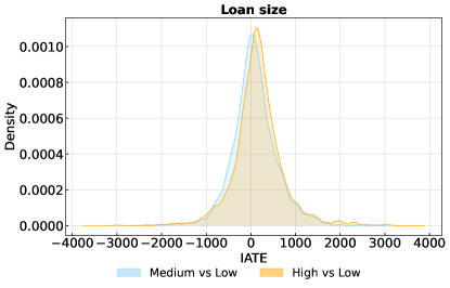
Figure 5: Distribution of IATE

Note: Means of the IATEs for the high (medium) vs low-interest rate groups: R78 (R163). Average standard errors of the IATEs for the high (medium) vs low-interest rate groups: R506 (R487).

As for the previous studies, we use Policy Trees of different depths and compare the welfare produced by the different allocations with the welfare from random and observed allocations. Due to this application’s relatively larger sample size, we also demonstrate the performance of both shallow and deeper trees. Additionally, we explore various combinations of trees: optimal, optimal with one final sequential optimal tree (+1), and optimal with two final sequential optimal trees (+2).

Policy Welfare (R) Treatment shares (%) Average returns Low rate Medium rate High rate Observed 497 39.84 28.40 31.75 Random 497 39.84 28.85 31.10 Unconstrained optimal Policy Tree     Depth-2 652 4.62 40.25 55.12     Depth-3 678 4.62 44.62 50.76     Depth-4 701 13.74 36.02 50.23 Unconstrained sequentially optimal Policy Trees     Depth-2+1 663 19.58 28.89 51.53     Depth-3+1 686 20.95 25.14 53.90     Depth-4+1 703 11.68 31.23 57.09     Depth-2+2 685 20.84 28.67 50.50     Depth-3+2 710 14.74 34.66 50.60     Depth-4+2 717 17.45 28.87 53.68 Note: The table shows the simulated and observed allocations of individuals per program under different policies. The outcome represents the average loan size in South African Rands (R7 = 1 USD).

Table 3: Treatment allocations Interest Rates and Loan Returns

Table 3 indicates that the observed and random allocations lead to the same welfare since the observed allocations are based on a stratified random assignment. The Table also shows that the Policy Trees increase welfare compared to the baseline policies, irrespective of the tree depth. Even implementing a Policy Tree of depth two demonstrates an increase in overall welfare by 31%, and deeper trees continue to yield improvements, although at a decreasing rate. The allocation pattern of the optimal Policy Trees shows that deeper trees tend to shift individuals away from the high-rate to a lower-risk group while increasing the average returns at the same time. The welfare estimated with the mixed trees (one or two sequential optimal final trees) is slightly lower than those obtained by the fully optimal tree. For example, the Optimal Policy Tree of depth four generates a welfare of R701, higher than R686 (R685) yielded by the depth-3+1 (depth 2+2) mixed Policy Tree.

Figure 6 shows the allocation rule for an optimal Policy Tree of depth 4, which combines both a large welfare improvement and policy rules that are relatively easy to interpret. As indicated in Table 3, the Policy Tree assigns roughly half of the sample to the high-rate treatment. Among this subgroup, the highest share (16% of the overall sample) falls between the ages of 35 and 43 and lacks higher education. Low-income individuals older than 53 also constitute a significant portion of the high-risk cohort (12% of the whole sample). The highest share of individuals assigned to the medium interest rate (14% of the sample) range from 28 to 32 years of age. The largest subgroup assigned to the low-rate group consists of high-income individuals older than 50 years (4.6% of the sample).

For detailed information on the treatment allocation rules for the other Policy Trees, we direct the reader to Section 5.2.3 of the Appendix.

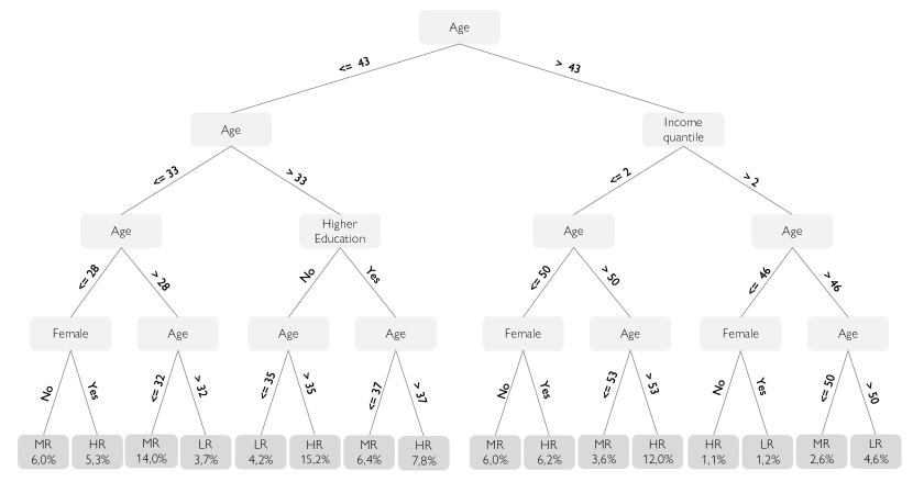
Figure 6: Allocation rule for an optimal Policy Tree of depth-4

Note: The policy tree shows the shares of individuals allocated to each treatment. The splitting variables of the tree are gender, age, income quantile and an indicator for achieved higher education. The final leaves of the trees indicate the treatments and corresponding shares of allocated individuals. LR: Low rate, MR: Medium rate, HR: High rate.

4 Technical considerations and conclusion

An optimal tree of arbitrary depth is computationally challenging due to its NP-hard nature. However, specifying a particular depth allows for polynomial-time resolution, making the depth of the tree a critical complexity parameter (Sverdrup, Kanodia, Zhou, Athey and Wager; 2020). Typically, estimating optimal trees beyond a depth of 4 (16 leaves) becomes challenging with moderate-sized training data. To improve computational performance, one option is to reduce the depth, sacrificing some efficiency for computational speed (and improved interpretability). Another option is to use sequential optimal trees. This means building a shallow initial tree, followed by a second shallow tree built from the sub-final leaves of the first one. Building the trees in sequence is much faster than constructing a single, deeper tree of the same overall depth. Alternatively, the minimum leaf size is crucial for performance optimisation. Setting leaf sizes too small can be impractical and increase computation times. Additionally, users can enhance speed by reducing the size of the training data at the cost of amplifying sampling noise. Another approach to enhancing speed is to limit the number of values considered during splitting. For continuous variables, the mcf algorithm evaluates by default only 100 equally spaced values, while it assesses 100 random combinations for categorical variables. Although this approximation improves computational efficiency, it may lead to some loss in accuracy, particularly as the data in the leaf nodes diminishes.

Furthermore, like predictive trees, policy trees can also exhibit instability regarding policy rules or welfare estimation. However, how to conduct inference about the stability of policy trees remains an open question in the literature. Athey and Wager (2021) propose a form of cross-validation to evaluate the accuracy of policy learning procedures, and they assess improvements over a random baseline. Similarly, Zhou et al. (2023) propose an alternative form of cross-validation and test whether optimal policy rules perform significantly better than sending all units to the same treatment. While the assessment of policy tree stability is not currently tackled in the present paper, future research efforts may concentrate on developing methods to evaluate this aspect effectively.

Despite this, the mcf ’s OptimalPolicy() class presents a notable advantage by providing a practical implementation of Policy Trees within multi-action settings, facilitating the creation of explainable assignment rules. Moreover, it offers best-scores and random allocation methods, which can be utilised for comparative welfare estimation. Notably, the integration of this class into the mcf package is advantageous. Indeed, it allows for the combination of causal machine learning estimates produced by the ModifiedCausalForest() as inputs for the policy tree, enhancing decision-making. The mcf package is an open-source Python package available on the Python Package Index (PyPI). The current work is based on version 0.5.1.

5 Appendix

5.1 Codebooks

Codebook for the Oregon health insurance study (Section 3.1)
Variable	Description
Table 3 – continued from previous page
variable	description
continued on next page
doc_any_12m	any primary care visits: survey data 12m
treatment	indicator equal to 1 if extracted for the lottery
age	in years, calculated as difference between 2008 and birth year
numhh_list	number of people in household on lottery list
draw	survey mailing wave for 0m survey
birthyear_list	birth year: lottery list data
have_phone_list	gave a phone number on lottery sign up: lottery list data
pobox_list	gave a PO Box as an address: lottery list data
english_list	individual requested english-language materials: lottery list data
female_list	indicator for female: lottery list data
zip_msa	zip code from lottery list is a metropolitan statistical area

Codebook for the Right Heart Catheterization (Section 3.2)
Variable	Description
Table 3 – continued from previous page
Variable	Description
continued on next page
adld3pc	index of activities of daily living 2 weeks prior to admission
age	age in years
alb1	albumin level in grams per deciliter
amihx	indicator for definite myocardial infarction
aps1	acute physiology and chronic health evaluation score (APACHE III)
bili1	bilirubin level in milligrams per deciliter
ca	cancer; 3 categories: metastatic cancer (Metastatic), no cancer (No), cancer (Yes)
card	indicator for cardiovascular diagnosis
cardiohx	indicator for acute myocardial infarction, peripheral vascular disease, severe, and very severe cardiovascular symptoms (NYHA-classes III and IV)
cat1	primary disease; 9 categories: acute respiratory failure (0), congestive heart failure (1), chronic obstructive pulmonary disease (2), cirrhosis (3), colon cancer metastatic to the liver (4), non-traumatic coma (5), non-small-cell cancer of the lung, stage III or IV (6), multiorgan system failure with malignancy (7), indicator for multiorgan system failure with sepsis (8)
cat2	secondary disease; 3 categories: missings or others (0), multiorgan system failure with malignancy (1), multiorgan system failure with sepsis(2)
cat2_miss	indicator for missings in cat2
chfhx	indicator for congestive heart failure
chrpulhx	indicator for chronic, severe, or very severe pulmonary disease
crea1	creatinine level in milligrams per deciliter
das2d3pc	Duke activity status index (DASI) two weeks before admission
dementhx	indicator for dementia, stroke or cerebral infarct, Parkinson’s disease
dnr1	indicator for do not resuscitate status on the first day
dth30	outcome indicator for mortality within 6 months
edu	education in years
gastr	indicator for gastrointestinal diagnosis
gibledhx	indicator for upper gastrointestinal bleeding
hema	indicator for hematologic diagnosis
hema1	hematocrit levels in percent
hrt1	heart rate in beats per minute
immunhx	indicator for immunosuppression, organ transplant, HIV positivity, diabetes mellitus with or without end organ damage, connective tissue disease
income	income in US dollars; 4 categories: below 11k (0), 11-25k (1), 25-50k (2), above 50k (3)
liverhx	indicator for cirrhosis, hepatic failure
malighx	indicator for solid tumor, metastatic disease, chronic leukemia/myeloma, acute leukemia, lymphoma
meanbp1	mean blood pressure in millimeters of mercury
meta	indicator for metabolic diagnosis
neuro	indicator for neurological diagnosis
ninsclas	medical insurance; 6 categories: Medicaid (0), Medicare (1), Medicare and Medicaid (2), no medical insurance (3), private medical insurance (4), private medical insurance and Medicaid (5)
ortho	indicator for orthopedic diagnosis
paco21	partial pressure of arterial carbon dioxide in millimeters of mercury
pafi1	ratio between partial pressure of arterial oxygen in millimeters of mercury and fraction of inspired oxygen
ph1	potential of hydrogen (pH) at logarithmic scale
pot1	blood potassium level in millimoles per liter
psychhx	indicator for psychiatric history, active psychosis or severe depression
race	race; 3 categories: African American (0), other race (1), Caucasian (2)
renal	indicator for renal diagnosis
renalhx	indicator for chronic renal disease, chronic hemodialysis, or peritoneal dialysis
resp	indicator for respiratory diagnosis
resp1	respiratory rate
scoma1	Glasgow coma score
seps	indicator for sepsis diagnosis
sex	indicator for gender (1=male)
sod1	sodium level in milliequivalents per liter
surv2md1	probability of surviving two months (based on support model estimations)
swang1	treatment indicator for right heart catheterisation
temp1	body temperature in degrees Celsius
transhx	indicator for transfer exceeding 24 hours from another hospital
trauma	indicator for trauma diagnosis
urin1	urine output per day in milliliters
urin1_miss	indicator for missings in urin1
wblc1	white blood cells in thousands per cubic millimeter
wtkilo1	weight in kilograms

Codebook for the Interest Rates and Loan Returns study (Section 3.3)
Variable	Description
Table 3 – continued from previous page
Variable	Description
continued on next page
adj_loan	loan size (loansize variable) multiplied by the interest rate (final4 variable) applied to calculate returns.
offer_risk	treatment, based on the original offered interest rate (offer4); offer_risk is equal to 1 for the offers with a value less than or equal to 7.75, indicating an associated low risk; offers with values greater than 7.75 but less than or equal to 9.75 are categorized as 2, associated to moderate risk; offers with a value greater than 9.75 are categorized as 3, associated to high risk.
age	age in years
dependants	number of individuals who rely on the primary household for economic support and care
qnt_income	quintiles of gross income
wave	number indicating in which wave the offer letter has been sent
risk_num	number from 1 to 3 indicating the client’s risk category
female	indicator for gender, equal to 1 if female
married	indicator for civil status, equal to 1 if married
edhi	indicator for higher education, equal to 1 if this level is achieved
rural	indicator for living in rural area

5.2 Policy Trees rules

This section shows policy rules for individuals allocated to treatment only. All tables indicate the splitting variables and related values produced by our Policy Trees. The codebooks in Section 5.1 provide the corresponding variable descriptions.

5.2.1 Policy rules Oregon Health Insurance Experiment

Table 4: Unconstrained optimal Policy Tree of depth-2

Splitting variables and values
female_list = 0, numhh_list = 1
female_list = 0, numhh_list $>$ 1
female_list = 0, age $\leq$ 47
female_list = 0, age $>$ 47

• Note: Policy rule for individuals assigned to Medicaid.

Table 5: Unconstrained optimal Policy Tree of depth-3

Splitting variables and values
age $\leq$ 50, age $\leq$ 31, age $\leq$ 26
age $\leq$ 50, age $\leq$ 31, age $>$ 26
age $\leq$ 50, age $>$ 31, age $\leq$ 38
age $\leq$ 50, age $>$ 31, age $>$ 38
age $>$ 50, numhh_list = 1, age $\leq$ 60
age $>$ 50, numhh_list = 1, age $>$ 60
age $>$ 50, numhh_list $>$ 1, age $\leq$ 59
age $>$ 50, numhh_list $>$ 1, age $>$ 59

• Note: Policy rule for individuals assigned to Medicaid.

Table 6: Constrained optimal Policy Tree of depth-2

Splitting variables and values
age $\leq$ 51, age $>$ 36
age $>$ 51, numhh_zip_msa = 0

• Note: Policy rule for individuals assigned to Medicaid.

Table 7: Unconstrained Optimal Policy Tree of depth-3

Splitting variables and values
numhh_list = 1, age $\leq$ 51, age $>$ 37
numhh_list = 1, age $>$ 51, zip_msa = 0
numhh_list $>$ 1, female_list = 0, age $>$ 25
numhh_list $>$ 1, female_list = 1, zip_msa = 0

• Note: Policy rule for individuals assigned to Medicaid.

Table 8: Constrained sequentially optimal Policy Trees of depth-2+1

Splitting variables and values
age $\leq$ 50, age $>$ 39, age $\leq$ 40
age $\leq$ 50, age $>$ 39, age $>$ 40
age $>$ 50, numhh_zip_msa = 0, age $\leq$ 53
age $>$ 50, numhh_zip_msa = 0, age $>$ 53
age $>$ 50, zip_msa = 1 numhh_list $>$ 1

• Note: Policy rule for individuals assigned to Medicaid.

Table 9: Constrained optimal Policy Tree of depth-4

numhh_list = 1, zip_msa = 0, female_list = 0, age $>$ 28
numhh_list = 1, zip_msa = 0, female_list $>$ 0.500, age $>$ 35
numhh_list = 1, zip_msa = 1, age $>$ 39, age $\leq$ 51
numhh_list $>$ 1, female_list = 0, zip_msa ¡ 0, age $\leq$ 36
numhh_list $>$ 1, female_list = 0 zip_msa = 0, age $>$ 36
numhh_list $>$ 1, female_list = 0, zip_msa = 1, age $>$ 28
numhh_list $>$ 1, female_list = 1, english_list = 0, age $\leq$ 42
numhh_list $>$ 1, female_list = 1, english_list = 1, zip_msa = 0

• Note: Policy rule for individuals assigned to Medicaid.

Table 10: Constrained sequentially optimal Policy Tree of depth-3+1

Splitting variables and values
numhh_list $>$ 1, female_list = 0, age $>$ 27
numhh_list = 1, age $\leq$ 51, age $>$ 37, age $<$ 39
numhh_list = 1, age $\leq$ 51, age $>$ 37, age $>$ 39
numhh_list = 1, age $>$ 51, zip_msa = 0, age $\leq$ 53
numhh_list = 1, age $>$ 51, zip_msa = 0, age $>$ 53
numhh_list $>$ 1, female_list = 1, zip_msa = 0, age $\leq$ 53
numhh_list $>$ 1, female_list = 1, zip_msa = 0, age $>$ 53
numhh_list $>$ 1, female_list = 1, zip_msa = 1, english_list = 0

• Note: Policy rule for individuals assigned to Medicaid.

5.2.2 Policy rules Right Heart Catheterization

Table 11: Unconstrained optimal Policy Tree of depth-2

Splitting variables and values
age $\leq$ 65, surv2md1 $\leq$ 0.480
age $>$ 65, surv2md1 $\leq$ 0.402

• Note: Policy rule for individuals assigned to RHC.

Table 12: Unconstrained optimal Policy Tree of depth-3

Splitting variables and values
cat1 in: 0 1 2 6 8, age $\leq$ 70, surv2md1 $\leq$ 0.450
cat1 in: 0 1 2 6 8, age $>$ 70, surv2md1 $\leq$ 0.402
cat1 not in: 0 1 2 6 8, cat1 in: 3 5, aps1 $>$ 64
cat1 not in: 0 1 2 6 8, cat1 not in: 3 5, surv2md1 $\leq$ 0.467

• Note: Policy rule for individuals assigned to RHC.

Table 13: Unconstrained sequentially optimal Policy Trees of depth-2+1

Splitting variables and values
age $\leq$ 65, surv2md1 $\leq$ 0.480, aps1 $\leq$ 80
age $\leq$ 65, surv2md1 $\leq$ 0.480, aps1 $>$ 80
age $>$ 65, surv2md1 $\leq$ 0.402, aps1 $>$ 50

• Note: Policy rule for individuals assigned to RHC.

Table 14: Unconstrained sequentially optimal Policy Trees of depth-3+1

Splitting variables and values
cat1 in: 0 2 8, age $\leq$ 69, surv2md1 $\leq$ 0.450, cat1 = 0
cat1 in: 0 2 8, age $\leq$ 69, surv2md1 $\leq$ 0.450, cat1 not in: 0
cat1 in: 0 2 8, age $>$ 69, surv2md1 $\leq$ 0.402, aps1 $>$ 61
cat1 not in: 0 2 8, cat1 in: 3 5, aps1 $>$ 64, aps1 $\leq$ 77
cat1 not in: 0 2 8, cat1 in: 3 5, aps1 $>$ 64, aps1 $>$ 77
cat1 not in: 0 2 8, cat1 not in: 3 5, surv2md1 $\leq$ 0.467, surv2md1 $\leq$ 0.384
cat1 not in: 0 2 8, cat1 not in: 3 5, surv2md1 $\leq$ 0.467, surv2md1 $>$ 0.384

• Note: Policy rule for individuals assigned to RHC.

5.2.3 Policy rules Interest Rates and Loan Returns

Table 15: Unconstrained Optimal Policy Tree of depth-2

Splitting variables and values	Treatment allocation
age $\leq$ 50, age $>$ 36	HR
age $>$ 50, qnt_income $\leq$ 2	HR
age $\leq$ 50, age $\leq$ 36	MR
age $>$ 50, qnt_income $>$ 2	LR

• Note: Policy rule for individuals assigned to HR: high rate, MR: medium rate and LR: low rate.

Table 16: Unconstrained optimal Policy Tree of depth-3

Splitting variables and values	Treatment allocation
age $>$ 46, qnt_income $>$ 2, age $>$ 50	LR
age $\leq$ 46, age $\leq$ 28, female = 0	MR
age $\leq$ 46, age $\leq$ 28, female = 1	HR
age $\leq$ 46, age $>$ 28, age $\leq$ 36	MR
age $>$ 46, qnt_income $\leq$ 2, age $\leq$ 53	MR
age $\leq$ 46, age $>$ 28, age $>$ 36	HR
age $>$ 46, qnt_income $\leq$ 2, age $>$ 53	HR
age $>$ 46, qnt_income $>$ 2, age $\leq$ 50	HR

• Note: Policy rule for individuals assigned to HR: high rate, MR: medium rate and LR: low rate.

Table 17: Unconstrained optimal Policy Tree of depth-4

Splitting variables and values	Treatment allocation
age $>$ 43, qnt_income $>$ 2, age $>$ 46, age $>$ 50	LR
age $\leq$ 43, age $\leq$ 33, age $>$ 28, age $>$ 32	LR
age $\leq$ 43, age $>$ 33, edhi = 0, age $\leq$ 35	LR
age $>$ 43, qnt_income $>$ 2, age $\leq$ 46, female =1	LR
age $\leq$ 43, age $\leq$ 33, age $\leq$ 28 female =1	MR
age $\leq$ 43, age $\leq$ 33, age $>$ 28, age $\leq$ 32	MR
age $\leq$ 43, age $>$ 33, edhi =1, age $\leq$ 37	MR
age $>$ 43, qnt_income $\leq$ 2, age $\leq$ 50, female = 0	MR
age $>$ 43, qnt_income $\leq$ 2, age $>$ 50, age $\leq$ 53	MR
age $\leq$ 43, age $\leq$ 33, age $\leq$ 28, female = 0	HR
age $\leq$ 43, age $>$ 33, edhi = 0, age $>$ 35	HR
age $\leq$ 43, age $>$ 33, edhi = 1, age $>$ 37	HR
age $>$ 43, qnt_income $\leq$ 2, age $\leq$ 50, female = 1	HR
age $>$ 43, qnt_income $\leq$ 2, age $>$ 50, age $>$ 53	HR
age $>$ 43, qnt_income $>$ 2, age $\leq$ 46, female = 0	HR
age $>$ 43, qnt_income $>$ 2, age $>$ 46, age $\leq$ 50	HR

• Note: Policy rule for individuals assigned to HR: high rate, MR: medium rate and LR: low rate.

Table 18: Unconstrained sequentially optimal Policy Trees of depth-2+1

Splitting variables and values	Treatment allocation
age $\leq$ 50, age $\leq$ 36, age $>$ 32	LR
age $>$ 50, qnt_income $>$ 2, age $\leq$ 57	LR
age $>$ 50, qnt_income $>$ 2, age $>$ 57	LR
age $\leq$ 50, age $\leq$ 36, age $\leq$ 32	MR
age $>$ 50, qnt_income $\leq$ 2, age $\leq$ 53	MR
age $\leq$ 50, age $>$ 36, age $\leq$ 38	HR
age $\leq$ 50, age $>$ 36, age $>$ 38	HR
age $>$ 50, qnt_income $\leq$ 2, age $>$ 53	HR

• Note: Policy rule for individuals assigned to HR: high rate, MR: medium rate and LR: low rate.

Table 19: Unconstrained sequentially optimal Policy Trees of depth-3+1

Splitting variables and values	Treatment allocation
age $\leq$ 46, age $\leq$ 28, female = 0, age $\leq$ 27	MR
age $\leq$ 46, age $\leq$ 28, female = 0., age $>$ 27	HR
age $\leq$ 46, age $\leq$ 28, female = 1, age $\leq$ 25	HR
age $\leq$ 46, age $\leq$ 28, female = 1, age $>$ 25	HR
age $\leq$ 46, age $>$ 28, age $\leq$ 36, age $\leq$ 32	MR
age $\leq$ 46, age $>$ 28, age $\leq$ 36, age $>$ 32	LR
age $\leq$ 46, age $>$ 28, age $>$ 36, age $\leq$ 37	HR
age $\leq$ 46, age $>$ 28, age $>$ 36, age $>$ 37	HR
age $>$ 46, qnt_income $\leq$ 2, age $\leq$ 53, qnt_income = 0	HR
age $>$ 46, qnt_income $\leq$ 2, age $\leq$ 53, qnt_income $>$ 0	MR
age $>$ 46, qnt_income $\leq$ 2, age $>$ 53, rural = 0	HR
age $>$ 46, qnt_income $\leq$ 2, age $>$ 53, rural = 1	HR
age $>$ 46, qnt_income $>$ 2, age $\leq$ 50, female = 0	LR
age $>$ 46, qnt_income $>$ 2, age $\leq$ 50, female = 1	HR
age $>$ 46, qnt_income $>$ 2, age $>$ 50, age $\leq$ 58	LR
age $>$ 46, qnt_income $>$ 2, age $>$ 50, age $>$ 58	LR

• Note: Policy rule for individuals assigned to HR: high rate, MR: medium rate and LR: low rate.

Table 20: Unconstrained sequentially optimal Policy Trees of depth-4+1

Splitting variables and values	Treatment
age $>$ 44, female = 0, qnt_income $>$ 2, age $\leq$ 50	HR
age $>$ 44, female = 0, qnt_income $>$ 2, age $>$ 50	LR
age $\leq$ 44, age $\leq$ 33, age $\leq$ 28, female = 0, age $\leq$ 27	MR
age $\leq$ 44, age $\leq$ 33, age $\leq$ 28, female = 0, age $>$ 27	HR
age $\leq$ 44, age $\leq$ 33, age $\leq$ 28, female = 1, age $\leq$ 25	HR
age $\leq$ 44, age $\leq$ 33, age $\leq$ 28, female = 1, age $>$ 25	HR
age $\leq$ 44, age $\leq$ 33, age $>$ 28, age $\leq$ 32, rural = 0	MR
age $\leq$ 44, age $\leq$ 33, age $>$ 28, age $\leq$ 32, rural = 1	MR
age $\leq$ 44, age $\leq$ 33, age $>$ 28, age $>$ 32, female = 0	LR
age $\leq$ 44, age $\leq$ 33, age $>$ 28, age $>$ 32, female = 1	LR
age $\leq$ 44, age $>$ 33, edhi = 0, age $\leq$ 35, qnt_income = 0	HR
age $\leq$ 44, age $>$ 33, edhi = 0, age $\leq$ 35, qnt_income $>$ 0	LR
age $\leq$ 44, age $>$ 33, edhi = 0, age $>$ 35, qnt_income $\leq$ 2	HR
age $\leq$ 44, age $>$ 33, edhi = 0, age $>$ 35, qnt_income $>$ 2	HR
age $\leq$ 44, age $>$ 33, edhi = 1, age $\leq$ 37, qnt_income = 0	MR
age $\leq$ 44, age $>$ 33, edhi = 1, age $\leq$ 37, qnt_income $>$ 0	MR
age $\leq$ 44, age $>$ 33, edhi = 1, age $>$ 37, rural = 0	HR
age $\leq$ 44, age $>$ 33, edhi = 1, age $>$ 37, rural = 1	HR
age $>$ 44, female = 0, qnt_income $\leq$ 2, age $\leq$ 53, qnt_income = 0	HR
age $>$ 44, female = 0, qnt_income $\leq$ 2, age $\leq$ 53, qnt_income $>$ 0	MR
age $>$ 44, female = 0, qnt_income $\leq$ 2, age $>$ 53, age $\leq$ 55	HR
age $>$ 44, female = 0, qnt_income $\leq$ 2, age $>$ 53, age $>$ 55	HR
age $>$ 44, female = 1 , age $\leq$ 53, age $\leq$ 50, age $\leq$ 47	HR
age $>$ 44, female = 1 , age $\leq$ 53, age $\leq$ 50, age $>$ 47	HR
age $>$ 44, female = 1 , age $\leq$ 53, age $>$ 50, edhi = 0	HR
age $>$ 44, female = 1 , age $\leq$ 53, age $>$ 50, edhi = 1	MR
age $>$ 44, female = 1 , age $>$ 53, edhi = 0, age $\leq$ 65	HR
age $>$ 44, female = 1 , age $>$ 53, edhi = 0, age $>$ 65	MR
age $>$ 44, female = 1 , age $>$ 53, edhi = 1, age $\leq$ 58	LR
age $>$ 44, female = 1 , age $>$ 53, edhi = 1, age $>$ 58	LR

• Note: Policy rule for individuals assigned to HR: high rate, MR: medium rate and LR: low rate.

Table 21: Unconstrained sequentially optimal Policy Trees of depth-2+2

Splitting variables and values	Treatment allocation
age $\leq$ 48, age $\leq$ 36, age $\leq$ 28, female = 0	MR
age $\leq$ 48, age $\leq$ 36, age $\leq$ 28, female $>$ 0	HR
age $\leq$ 48, age $\leq$ 36, age $>$ 28, age $\leq$ 32	MR
age $\leq$ 48, age $\leq$ 36, age $>$ 28, age $>$ 32	LR
age $\leq$ 48, age $>$ 36, female = 0, age $\leq$ 46	HR
age $\leq$ 48, age $>$ 36, female = 0, age $>$ 46	MR
age $\leq$ 48, age $>$ 36, female $>$ 0, age $\leq$ 37	MR
age $\leq$ 48, age $>$ 36, female $>$ 0, age $>$ 37	HR
age $>$ 48, qnt_income $\leq$ 2, qnt_income = 0, age $\leq$ 52	HR
age $>$ 48, qnt_income $\leq$ 2, qnt_income = 0, age $>$ 52	HR
age $>$ 48, qnt_income $\leq$ 2, qnt_income $>$ 0, age $\leq$ 53	MR
age $>$ 48, qnt_income $\leq$ 2, qnt_income$>$ 0, age $>$ 53	HR
age $>$ 48, qnt_income $>$ 2, age $\leq$ 51	LR
age $>$ 48, qnt_income $>$ 2, age $>$ 51	LR

• Note: Policy rule for individuals assigned to HR: high rate, MR: medium rate and LR: low rate.

Table 22: Unconstrained sequentially optimal Policy Trees of depth-3+2

Splitting variables and values	Treatment
	allocation
age $\leq$ 44, age $\leq$ 28, female = 0, age $\leq$ 26, qnt_income $\leq$ 1	MR
age $\leq$ 44, age $\leq$ 28, female = 0, age $\leq$ 26, qnt_income $>$ 1	MR
age $\leq$ 44, age $\leq$ 28, female = 0, age $>$ 26, qnt_income $\leq$ 1	HR
age $\leq$ 44, age $\leq$ 28, female = 0, age $>$ 26, qnt_income $>$ 1	MR
age $\leq$ 44, age $\leq$ 28, female = 1, qnt_income $\leq$ 1, qnt_income = 0	HR
age $\leq$ 44, age $\leq$ 28, female = 1, qnt_income $\leq$ 1, qnt_income $>$ 0	HR
age $\leq$ 44, age $\leq$ 28, female =1 , qnt_income $>$ 1, qnt_income $\leq$ 2.5	HR
age $\leq$ 44, age $\leq$ 28, female $>$ 1, qnt_income $>$ 1, qnt_income $>$ 2.5	HR
age $\leq$ 44, age $>$ 28, age $\leq$ 36, age $\leq$ 33, age $\leq$ 32	MR
age $\leq$ 44, age $>$ 28, age $\leq$ 36, age $\leq$ 33, age $>$ 32	LR
age $\leq$ 44, age $>$ 28, age $\leq$ 36, age $>$ 33, edhi = 0	LR
age $\leq$ 44, age $>$ 28, age $\leq$ 36, age $>$ 33, edhi = 1	MR
age $\leq$ 44, age $>$ 28, age $>$ 36, female = 0, qnt_income $\leq$ 1	HR
age $\leq$ 44, age $>$ 28, age $>$ 36, female = 0, qnt_income $>$ 1	HR
age $\leq$ 44, age $>$ 28, age $>$ 36, female = 1 , qnt_income $\leq$ 2	HR
age $\leq$ 44, age $>$ 28, age $>$ 36, female = 1 , qnt_income $>$ 2.	MR
age $>$ 44, qnt_income $\leq$ 2, female = 0, age $\leq$ 55, qnt_income = 0	HR
age $>$ 44, qnt_income $\leq$ 2, female = 0, age $\leq$ 55, qnt_income $>$ 0	MR
age $>$ 44, qnt_income $\leq$ 2, female = 0, age $>$ 55, age $\leq$ 61	HR
age $>$ 44, qnt_income $\leq$ 2, female = 0, age $>$ 55, age $>$ 61	HR
age $>$ 44, qnt_income $\leq$ 2, female = 1, age $\leq$ 50, age $\leq$ 46	HR
age $>$ 44, qnt_income $\leq$ 2, female = 1 , age $\leq$ 50, age $>$ 46	HR
age $>$ 44, qnt_income $\leq$ 2, female = 1 , age $>$ 50, age $\leq$ 53	MR
age $>$ 44, qnt_income $\leq$ 2, female = 1 , age $>$ 50, age $>$ 53	HR
age $>$ 44, qnt_income $>$ 2, age $\leq$ 50, age $\leq$ 47	HR
age $>$ 44, qnt_income $>$ 2, age $\leq$ 5 age $>$ 47	HR
age $>$ 44, qnt_income $>$ 2, age $>$ 50, age $\leq$ 59	LR
age $>$ 44, qnt_income $>$ 2, age $>$ 50, age $>$ 59	LR

• Note: Policy rule for individuals assigned to HR: high rate, MR: medium rate and LR: low rate.

Table 23: Unconstrained sequentially optimal Policy Trees of depth-4+2

Splitting variables and values	Treatment
	allocation
age $\leq$ 44, age $\leq$ 33, age $\leq$ 28, female = 0, age $\leq$ 26, qnt_income $\leq$ 1	MR
age $\leq$ 44, age $\leq$ 33, age $\leq$ 28, female = 0, age $\leq$ 26, qnt_income $>$ 1	MR
age $\leq$ 44, age $\leq$ 33, age $\leq$ 28, female = 0, age $>$ 26, qnt_income $\leq$ 1	HR
age $\leq$ 44, age $\leq$ 33, age $\leq$ 28, female = 0, age $>$ 26, qnt_income $>$ 1	MR
age $\leq$ 44, age $\leq$ 33, age $\leq$ 28, female $>$ 1, qnt_income $\leq$ 1, qnt_income = 0	HR
age $\leq$ 44, age $\leq$ 33, age $\leq$ 28, female = 1, qnt_income $\leq$ 1, qnt_income $>$ 0	HR
age $\leq$ 44, age $\leq$ 33, age $\leq$ 28, female = 1, qnt_income $>$ 1, qnt_income $\leq$ 2.5	HR
age $\leq$ 44, age $\leq$ 33, age $\leq$ 28, female = 1, qnt_income $>$ 1, qnt_income $>$ 2.5	HR
age $\leq$ 44, age $\leq$ 33, age $>$ 28, age $\leq$ 32, edhi = 0, age $\leq$ 30	MR
age $\leq$ 44, age $\leq$ 33, age $>$ 28, age $\leq$ 32, edhi = 0, age $>$ 30	HR
age $\leq$ 44, age $\leq$ 33, age $>$ 28, age $\leq$ 32, edhi = 1, qnt_income = 0	HR
age $\leq$ 44, age $\leq$ 33, age $>$ 28, age $\leq$ 32, edhi = 1, qnt_income $>$ 0	MR
age $\leq$ 44, age $\leq$ 33, age $>$ 28, age $>$ 32, female = 0	LR
age $\leq$ 44, age $\leq$ 33, age $>$ 28, age $>$ 32, female $>$ 0	LR
age $\leq$ 44, age $>$ 33, edhi = 0, age $\leq$ 35, qnt_income = 0	HR
age $\leq$ 44, age $>$ 33, edhi = 0, age $\leq$ 35, qnt_income $>$ 0	LR
age $\leq$ 44, age $>$ 33, edhi = 0, age $>$ 35, qnt_income $\leq$ 2, age $\leq$ 36	LR
age $\leq$ 44, age $>$ 33, edhi = 0, age $>$ 35, qnt_income $\leq$ 2, age $>$ 36	HR
age $\leq$ 44, age $>$ 33, edhi = 0, age $>$ 35, qnt_income $>$ 2, age $\leq$ 39	HR
age $\leq$ 44, age $>$ 33, edhi = 0, age $>$ 35, qnt_income $>$ 2, age $>$ 39	HR
age $\leq$ 44, age $>$ 33, edhi = 1, age $\leq$ 37, qnt_income $\leq$ 2, qnt_income $\leq$ 1	MR
age $\leq$ 44, age $>$ 33, edhi = 1, age $\leq$ 37, qnt_income $\leq$ 2, qnt_income $>$ 1	LR
age $\leq$ 44, age $>$ 33, edhi = 1, age $\leq$ 37, qnt_income $>$ 2, female = 0	MR
age $\leq$ 44, age $>$ 33, edhi = 1, age $\leq$ 37 qnt_income $>$ 2, female = 1	MR
age $\leq$ 44, age $>$ 33, edhi = 1, age $>$ 37, qnt_income $\leq$ 2, qnt_income $\leq$ 1	HR
age $\leq$ 44 age $>$ 33, edhi = 1, age $>$ 37, qnt_income $\leq$ 2, qnt_income   1	HR
age $\leq$ 44, age $>$ 33, edhi = 1, age $>$ 37, qnt_income $>$ 2, female = 0	HR
age $\leq$ 44, age $>$ 33, edhi = 1, age $>$ 37, qnt_income $>$ 2, female = 1	MR
age $>$ 44, qnt_income $\leq$ 1, age $\leq$ 52, female = 0, qnt_income = 0	HR
age $>$ 44, qnt_income $\leq$ 1 age $\leq$ 52, female = 0, qnt_income $>$ 0	MR
age $>$ 44, qnt_income $\leq$ 1, age $\leq$ 52, female = 1, age $\leq$ 47, qnt_income = 0	HR
age $>$ 44, qnt_income $\leq$ 1, age $\leq$ 52, female = 1 , age $\leq$ 47, qnt_income $>$ 0	MR
age $>$ 44, qnt_income $\leq$ 1, age $\leq$ 52, female = 1 , age $>$ 47, qnt_income = 0	MR
age $>$ 44, qnt_income $\leq$ 1 age $\leq$ 52, female= 1, age $>$ 47, qnt_income $>$ 0	MR
age $>$ 44, qnt_income $\leq$ 1, age $>$ 52, age $\leq$ 60, qnt_income = 0, age $\leq$ 56	HR
age $>$ 44, qnt_income $\leq$ 1, age $>$ 52, age $\leq$ 60, qnt_income = 0, age $>$ 56	HR
age $>$ 44, qnt_income $\leq$ 1, age $>$ 52, age $\leq$ 60, qnt_income $>$ 0, age $\leq$ 55	MR
age $>$ 44, qnt_income $\leq$ 1, age $>$ 52, age $\leq$ 60, qnt_income $>$ 0, age $>$ 55	HR
age $>44$, qnt_income $\leq 1$, age $>52$, age $>60$, age $\leq 65$, age $\leq 62$	HR
age $>44$, qnt_income $\leq 1$, age $>52$, age $>60$, age $\leq 65$, age $>62$	HR
age $>44$, qnt_income $\leq 1$, age $>52$, age $>60$, age $>65$, age $\leq 68$	HR
age $>44$, qnt_income $\leq 1$, age $>52.$, age $>60$, age $>65$, age $>68$	HR
age $>44$, qnt_income $>1$, qnt_income $\leq 2.5$, female = 0, age $\leq 55$, age $\leq 50$	MR
age $>44$, qnt_income $>1$, qnt_income $\leq 2.5$, female = 0, age $\leq 55$, age $>50$	MR
age $>44$, qnt_income $>1$, qnt_income $\leq 2.5$, female = 0, age $>55$, age $\leq 60$	LR
age $>44$, qnt_income $>1$, qnt_income $\leq 2.5$, female = 0, age $>55$, age $>60$	HR
age $>44$, qnt_income $>1$, qnt_income $\leq 2.5$, female = 1, age $\leq 53$, age $\leq 48$	HR
age $>44$, qnt_income $>1$, qnt_income $\leq 2.5$, female = 1, age $\leq 53$, age $>48$	MR
age $>44$, qnt_income $>1$, qnt_income $\leq 2.5$, female = 1, age $>53$, age $\leq 62$	HR
age $>44$, qnt_income $>1$, qnt_income $\leq 2.5$, female = 1, age $>53$, age $>62$	HR
age $>44$, qnt_income $>1$, qnt_income $>2.5$, age $\leq 50$, age $\leq 46$, female = 0	HR
age $>44$, qnt_income $>1$, qnt_income $>2.5$, age $\leq 50$, age $\leq 46$, female = 1	LR
age $>44$, qnt_income $>1$, qnt_income $>2.5$, age $\leq 50$, age $>46$, female = 0	LR
age $>44$, qnt_income $>1$, qnt_income $>2.5$, age $\leq 50$, age $>46$, female $>0$	HR
age $>44$, qnt_income $>1$, qnt_income $>2.5$, age $>50$, age $\leq 55$, female = 0	LR
age $>44$, qnt_income $>1$, qnt_income $>2.5$, age $>50$, age $\leq 55$, female = 1	LR
age $>44$, qnt_income $>1$, qnt_income $>2.5$, age $>50$, age $>55$, female = 0	LR
age $>44$, qnt_income $>1$, qnt_income $>2.5$, age $>50$, age $>55$, female = 1	LR

• Note: Policy rule for individuals assigned to HR: high rate, MR: medium rate and LR: low rate.

References

- (1)
- Athey and Wager (2021) Athey, S. and Wager, S. (2021). Policy learning with observational data, Econometrica 89(1): 133–161.
- Baicker et al. (2017) Baicker, K., Allen, H. L., Wright, B. J. and Finkelstein, A. N. (2017). The effect of medicaid on medication use among poor adults: evidence from oregon, Health Affairs 36(12): 2110–2114.
- Baicker and Finkelstein (2018) Baicker, K. and Finkelstein, A. (2018). The impact of medicaid expansion on voter participation: evidence from the oregon health insurance experiment, Technical report, National Bureau of Economic Research.
- Baicker et al. (2014) Baicker, K., Finkelstein, A., Song, J. and Taubman, S. (2014). The impact of health insurance expansions on other social safety net programs, American Economic Review 104(5): 322–328.
- Baicker et al. (2013) Baicker, K., Taubman, S. L., Allen, H. L., Bernstein, M., Gruber, J. H., Newhouse, J. P., Schneider, E. C., Wright, B. J., Zaslavsky, A. M. and Finkelstein, A. N. (2013). The oregon experiment—effects of medicaid on clinical outcomes, New England Journal of Medicine 368(18): 1713–1722.
- Bodory et al. (2022) Bodory, H., Busshoff, H. and Lechner, M. (2022). High resolution treatment effects estimation: Uncovering effect heterogeneities with the modified causal forest, Entropy 24(8): 1039.
- Carcillo and Grubb (2006) Carcillo, S. and Grubb, D. (2006). From inactivity to work, (36).
- Connors et al. (1996) Connors, A. F., Speroff, T., Dawson, N. V., Thomas, C., Harrell, F. E., Wagner, D., Desbiens, N., Goldman, L., Wu, A. W., Califf, R. M. et al. (1996). The effectiveness of right heart catheterization in the initial care of critically iii patients, Jama 276(11): 889–897.
- Finkelstein et al. (2019) Finkelstein, A., Hendren, N. and Luttmer, E. F. (2019). The value of medicaid: Interpreting results from the oregon health insurance experiment, Journal of Political Economy 127(6): 2836–2874.
- Finkelstein et al. (2016) Finkelstein, A. N., Taubman, S. L., Allen, H. L., Wright, B. J. and Baicker, K. (2016). Effect of medicaid coverage on ed use—further evidence from oregon’s experiment.
- Finkelstein et al. (2012) Finkelstein, A., Taubman, S., Wright, B., Bernstein, M., Gruber, J., Newhouse, J. P., Allen, H., Baicker, K. and Oregon Health Study Group, t. (2012). The oregon health insurance experiment: evidence from the first year, The Quarterly journal of economics 127(3): 1057–1106.
- Hastie et al. (2009) Hastie, T., Tibshirani, R. and Friedman, J. (2009). The Elements of Statistical Learning: Data Mining, Inference, and Prediction, Springer series in statistics, Springer.
- Imbens and Wooldridge (2009) Imbens, G. W. and Wooldridge, J. M. (2009). Recent developments in the econometrics of program evaluation, Journal of Economic Literature 47(1): 5–86.
- Kallus and Zhou (2021) Kallus, N. and Zhou, A. (2021). Fairness, welfare, and equity in personalized pricing, Proceedings of the 2021 ACM conference on fairness, accountability, and transparency, pp. 296–314.
- Karlan and Zinman (2008) Karlan, D. S. and Zinman, J. (2008). Credit elasticities in less-developed economies: Implications for microfinance, American Economic Review 98(3): 1040–1068.
- Keele and Small (2018) Keele, L. and Small, D. S. (2018). Pre-analysis plan for a comparison of matching and black box-based covariate adjustment, Observational Studies 4(1): 97–110.
- Keele and Small (2021) Keele, L. and Small, D. S. (2021). Comparing covariate prioritization via matching to machine learning methods for causal inference using five empirical applications, The American Statistician 75(4): 355–363.
- Kitagawa and Tetenov (2018) Kitagawa, T. and Tetenov, A. (2018). Who should be treated? empirical welfare maximization methods for treatment choice, Econometrica 86(2): 591–616.
- Kitagawa and Tetenov (2021) Kitagawa, T. and Tetenov, A. (2021). Equality-minded treatment choice, Journal of Business & Economic Statistics 39(2): 561–574.
- Knaus et al. (1995) Knaus, W. A., Harrell, F. E., Lynn, J., Goldman, L., Phillips, R. S., Connors, A. F., Dawson, N. V., Fulkerson, W. J., Califf, R. M., Desbiens, N. et al. (1995). The support prognostic model: Objective estimates of survival for seriously ill hospitalized adults, Annals of internal medicine 122(3): 191–203.
- Lechner and Mareckova (2024) Lechner, M. and Mareckova, J. (2024). Comprehensive causal machine learning.
- Manski (2004) Manski, C. F. (2004). Statistical treatment rules for heterogeneous populations, Econometrica 72(4): 1221–1246.
- Mbakop and Tabord-Meehan (2021) Mbakop, E. and Tabord-Meehan, M. (2021). Model selection for treatment choice: Penalized welfare maximization, Econometrica 89(2): 825–848.
- Ramsahai et al. (2011) Ramsahai, R. R., Grieve, R. and Sekhon, J. S. (2011). Extending iterative matching methods: an approach to improving covariate balance that allows prioritisation, Health Services and Outcomes Research Methodology 11: 95–114.
- Sverdrup et al. (2020) Sverdrup, E., Kanodia, A., Zhou, Z., Athey, S. and Wager, S. (2020). policytree: Policy learning via doubly robust empirical welfare maximization over trees, Journal of Open Source Software 5(50): 2232.
- Sverdrup et al. (2023) Sverdrup, E., Kanodia, A., Zhou, Z., Athey, S. and Wager, S. (2023). policytree: Policy learning via doubly robust empirical welfare maximization over trees, Comprehensive R Archive Network .
- Zhou et al. (2023) Zhou, Z., Athey, S. and Wager, S. (2023). Offline multi-action policy learning: Generalization and optimization, Operations Research 71(1): 148–183.