Limits of isotropic damage models for complex load paths — beyond stress triaxiality and Lode angle parameter
Abstract
The stress triaxiality and the Lode angle parameter are two well established stress invariants for the characterization of damage evolution. This work assesses the limits of this tuple by using it for damage predictions via ductile damage models from continuum damage mechanics. Isotropic and anisotropic formulations of two well-established models are used to avoid model-specific restrictions. The damage evolution is analyzed for different load paths, while the stress triaxiality and the Lode angle parameter are controlled. The equivalent plastic strain is moreover added as a third parameter. These analyses reveal that this triple does still not suffice to uniquely define the damage state. As a consequence, well-established concepts such as fracture surfaces depending on this triple have to be taken with care, if complex paths are to be investgated. These include, e.g., load paths observed during metal forming applications with varying load directions or multiple stages.
keywords:
damage, triaxiality, lode angle, path dependence1 Introduction
The prediction of damage in materials is still a major challenge in many engineering disciplines since the underlying mechanisms are even nowadays not fully understood. As a result, large safety factors are mandatory to statistically ensure the functionality of structures and components. The modeling of the underlying material behavior is thus a key aspect for understanding and predicting the performance of these parts, cf. [1, 2, 3].
From a microscopic view, the mechanism of ductile damage can be related to the nucleation, the growth and finally the coalescence of voids induced by plastic deformation [4]. Depending on the material of interest, voids can show different origins and shapes, e.g., decohesion at hard particles. Since voids reduce the effective (load-carrying) area, they result in a reduced effective material stiffness [5], which ultimately also reduces the load-bearing capacity of the material. A natural modeling framework is thus the effective stress concept, cf. [6, 7]. Within this concept, which is also known as principle of strain equivalence, the true stresses are introduced. They are defined with respect to the effective cross sectional area caused by void nucleation, growth and coalescence. An alternative modeling concept is based on effective strains, which can be interpreted as the decomposition of the total strains into elastic and damage-related parts [8, 9]. Finally, an effective damage-induced elastic stiffness can also be derived by means of the concept of strain energy equivalence [10, 11]. In contrast to the concept of effective stresses and the concept of effective strains, the variational principle of strain energy equivalence naturally enforces physically relevant invariances. For instance, it naturally leads to a symmetric Cauchy stress even for anisotropic damage degradation (certainly, provided a Boltzmann continuum is considered).
Turning the view to the macroscopic description, a common approach for damage characterization is based on stress invariants like triaxiality and Lode angle parameter
| (1) | ||||
| (2) |
combined with an equivalent plastic strain, cf. [12, 13], via
| (3) |
Value is the Lode parameter and the stress eigenvalues. Moreover, corresponds to the plastic strain rate tensor. From a mathematical point of view the aforementioned characterization corresponds to an isotropic approximation. Early research showed that the stress triaxiality can be related to the physical process of void nucleation, growth and coalescence, cf. [14, 15]. Likewise, the Lode angle parameter was found to characterize damage evolution at low stress triaxialities, see [13]. More recently, the Lode angle parameter has been investigated for different fracture criteria in order to characterize the onset of damage [16]. Additional influences of the complete stress state on the damage evolution are often not considered, for instance, those accounting for anisotropic behavior. Moreover, the triple of stress triaxiality, Lode angle parameter and equivalent plastic strain often changes in time for complex load paths. Therefore, such load paths – as occuring in forming processes [17] – require an extended description. The present work thus analyzes the limits of simplified isotropic damage characterizations such as that given by Eqs. (1)–(3) and identifies suitable and unsuitable load conditions.
The focus of this work is on ductile damage in the context of continuum damage mechanics. The key highlights are:
-
1.
The frequently applied recommendation ”the lower the stress triaxiality, the lower the damage accumulation” is shown to be wrong for certain complex load paths.
-
2.
Such load paths are identified by means of computational optimization.
-
3.
An improved characterization of damage by means of the stress triaxiality, the Lode (angle) parameter as well as the equivalent plastic strains, as employed in the concept of fracture surfaces [13], is shown to be still insufficient.
-
4.
Finally, even a characterization of damage by a complete isotropic representation of the stress tensor (all invariants) is demonstrated to be to inaccurate for complex load paths.
In order to elaborate these highlights, two general anisotropic damage models depending on the complete stress tensor are considered and subsequently simplified in a controlled manner. For instance, the prediction capabilities of the models for two different load paths with identical stress triaxialities and/or Lode angle parameters are compared. Since such numerical experiments may also depend on the underlying constitutive model, two different modeling frameworks are adopted. While the first is based on the principle of energy equivalence [10, 18, 11], the latter is the by now classic Lemaitre model [19].
This work is structured as follows. Section 2 describes two constitutive models based on continuum damage mechanics, which form the basis for the subsequent investigations. Numerical methods in order to discretize, control and optimize load paths are presented in Section 3. Particularly, techniques for prescribing the stress-triaxiality and the Lode (angle) parameter are presented. The main findings are reported in Section 4. It covers numerical experiments highlighting the limits of different isotropic damage characterizations.
2 Continuum damage mechanics – two prototype models
Two constitutive models are briefly presented for the prediction of ductile damage, both as isotropic and anisotropic formulations. This allows a comprehensive load path analysis that is not bound to the characteristics of a single model. The two models are characteristic prototypes of the effective configuration concept (also known by the principle of strain energy equivalence) and the effective stress concept (also known by the principle of strain equivalence). While model ECC is based on the principle of strain energy equivalence, model LEM (Lemaitre model) falls into the range of the principle of strain equivalence. All models are calibrated with the same experimental data and form the basis for the subsequent numerical investigations.
2.1 ECC-Model – Effective Configuration Concept
The first model is based on the concept of strain energy equivalence, cf. [10]. The constitutive relations are adopted from the works in [11, 18]. The Helmholtz energy is additively decomposed into an elastic part () and a plastic part () according to
| (4) | ||||
| (5) | ||||
| (6) |
The strain tensor is also additively decomposed into an elastic and a plastic part, i.e., , cf. [20].
The model captures isotropic as well as kinematic hardening due to the state variables and , respectively.
Here, isotropic hardening is captured by a tensorial internal variable, following the principle of strain energy equivalence [11]. Both the elastic and the plastic energy contribution are affected by the damage evolution due to integrity tensor . The integrity tensor can be interpreted as an inverse damage measure, i.e., represents the virgin material, while some of the eigenvalues of converge to zero for completely damaged material points. By choosing , Hooke’s law is recovered. Accordingly, and are the Lame parameters. Furthermore, is the isotropic hardening modulus and is the kinematic hardening modulus.
A crucial contribution to the material model is the micro-closure-reopening (MCR) effect, which only allows damage evolution under tensile modes. Within the present model, the MCR effect is incorporated through an additive decomposition of the elastic strain tensor into its tensile and its compression states according to
| (7) |
Here, are the eigenvalues, are the eigenprojections of the elastic strain tensor and is the Heaviside function. Within the numerical implementation, the discontinuous Heaviside function has been approximated in line with [11] by setting numerical parameters , and . A straightforward calculation of the thermodynamic driving forces leads to
| (8) | ||||
| (9) | ||||
| (10) | ||||
| (11) | ||||
| (12) | ||||
| (13) |
where is the stress tensor, is the back stress tensor, is the drag stress tensor and the energy release rate. Using the thermodynamic driving forces, the dissipation inequality reads in its reduced form
| (14) |
By following the principle of Generalized Standard Materials [21], a plastic potential is introduced for the definition of the evolution equations. The dissipation inequality is known to be automatically fulfilled if that potential is convex, non-negative and contains the origin. That potential is specified as
| (15) |
and consists of the yield function and non-associated parts and . The yield function is chosen as
| (16) | ||||
| (17) |
where the equivalent stress is of von Mises-type and depends on the relative stress tensor . According to Eq. (16), the yield function captures linear and exponential isotropic hardening. The respective model parameters are denoted as , and . The non-associative parts of potential (15) are given as
| (18) | ||||
| (19) |
and extend the model to non-linear kinematic hardening of Armstrong-Frederick type with model parameter , cf. [22]. The damage evolution is controlled by potential and consists of an isotropic part (damage modulus ) and an anisotropic part (damage modulus ). The damage exponent allows for greater flexibility when calibrating the model to experiments. Furthermore, potential depends only on the elastic part of the energy release rate . This novel modification of the original model ensures that no damage evolution occurs under compression. The evolution equations follow as gradients of plastic potential (15) – in line with the principle of Generalized Standard Materials – and read
| (20) |
which concludes the constitutive model.
Isotropic model
By setting , an isotropic damage model is obtained. This case will also be employed within the numerical experiments.
2.2 LEM-Model – Effective Stress Concept (Lemaitre model)
The second model is adopted from [19] and is based on the principle of strain equivalence. Gibbs energy is specified as
| (21) | ||||
| (22) | ||||
| (23) |
and depends on model parameters Young’s modulus , Poisson’s ratio , damage parameter , the isotropic hardening parameters and , and the kinematic hardening modulus . The additive decomposition of the total strains into elastic and plastic parts is again considered as . Furthermore, the stress tensor is decomposed into a deviatoric () and a hydrostatic part () and subsequently into their respective positive and negative parts in order to capture the MCR-effect. Strain-like variables and are suitable for kinematic and isotropic hardening, respectively. The damage evolution is captured by means of second-order tensor , which enters energy (22) in terms of variables
While undamaged material is represented by , at least one eigenvalue of converges to one for completely damaged material points.
The thermodynamic driving forces follow as the derivatives of and read
| (24) | ||||
| (25) | ||||
| (26) | ||||
| (27) |
The transformation of Gibbs energy into Helmholtz energy reads
| (28) |
and allows to derive the reduced dissipation inequality as
| (29) |
Following the principle of Generalized Standard Materials once again, plastic potential is specified. Analogously to the previous model, is assumed to be of type
| (30) |
with von Mises-type yield function
| (31) |
and initial yield limit . The non-associative part of potential (30) extends the model to non-linear kinematic hardening and reads
| (32) |
with the non-linear kinematic hardening parameter . The evolution equations then result in
| (33) |
The evolution equation for damage tensor is adopted from an isotropic potential-based formulation by assuming that the rate of the damage tensor is given by the rate of the plastic strains, cf. [19]. To be more specific,
| (34) | ||||
| (35) |
with model parameters and . Moreover, the evolution is formulated by means of a scalar-valued energy release rate , where norm applies the absolute value to each component of the tensor.
Isotropic model
The isotropic version of this model results through the modification of eq. (34) into its spherical counterpart. Here, the choice
| (36) |
is made by utilizing Eq. (3). This choice has been made since it leads to similar results as the underlying anisotropic model when considering a uniaxial tensile test.
2.3 Model calibration
All four models the isotropic and the anisotropic ECC model (ECC-i and ECC-a) as well as the isotropic and the anisotropic LEM model (LEM-i and LEM-a) are calibrated to experimental data from [23] for comparability and a link to applications in forming technology. The tensile test of case-hardened steel 16MnCrS5 up to strain amplitudes of forms the basis. For this range of deformation, the strains are spatially homogeneous and necking does not occur. Both models, the anisotropic ECC model (ECC-a) and the anisotropic LEM model (LEM-a) were calibrated by means of a standard least-squares approach, while elastic parameters and and the initial yield stress were calculated beforehand. Subsequently, the isotropic models (ECC-i and LEM-i) were considered where for the sake of comparison only the damage-related parameters were recalibrated. A visualization of the calibrations is shown in Fig. 1 and the final list of model parameters is given in Tab. 1 and 2.
| Parameter name | Symbol | Value | Unit |
| First Lame parameter | |||
| Second Lame parameter | |||
| Yield stress | |||
| Kinematic hardening modulus | |||
| Armstrong-Frederick extension | - | ||
| Isotropic hardening modulus | |||
| Isotropic hardening increment | |||
| Isotropic hardening parameter | |||
| Anisotropic (ECC-a model) | |||
| Isotropic damage modulus | |||
| Anisotropic damage modulus | |||
| Damage exponent | - | ||
| Isotropic (ECC-i model) | |||
| Isotropic damage modulus | |||
| Anisotropic damage modulus | |||
| Damage exponential | - | ||
| Parameter name | Symbol | Value | Unit |
| First Lame parameter | |||
| Second Lame parameter | |||
| Yield stress | |||
| Isotropic hardening parameter | - | ||
| Kinematic hardening modulus | |||
| Nonlinear kinematic parameter | |||
| Saturation hardening stress | |||
| Anisotropic (LEM-a model) | |||
| Damage parameter | - | ||
| Damage scale | |||
| Damage exponent | - | ||
| Isotropic (LEM-i model) | |||
| Damage parameter | - | ||
| Damage scale | |||
| Damage exponent | - | ||
Both models match the experimental data well, see Figure 1 (a).
The largest error between the experiments and the calibration is associated with the LEM-a model and occurs at a strain of . However, the respective error is below and hence, less than . The behavior with respect to a shear mode is additionally shown in Figure 1 (c) in order to highlight the models’ different response – the shear mode was not part of the calibration. Both models show qualitatively similar behavior with a maximum deviation of less than . It shall be underlined that different models are used for a better and model-independent interpretation of the results. An evaluation of the individual models themselves is not intended and clearly depends on the intended application.
Remark 1
The constitutive models are evaluated at the material point level due to the spatially constant stress and strain field (no necking). Therefore, no regularization is required. If boundary value problems with localization are to be analyzed, a micromorphic regularization in order to render finite element simulations well-posed is included in the models. The respective energy contributions are, however, disregarded in this work, cf. [24, 25].
3 Methodology of evaluation: load path parametrization and damage measures
The analysis of various load paths is a key of the present evaluation of damage descriptions. For that reason, the parametrization of the load paths is explained in the following Subsection 3.1. As one example of the various enforced stress and/or strain paths, the predictions of the previously introduced models will be compared along identical stress triaxialities and/or Lode angle parameters. Characteristic damage measures are furthermore defined in Subsection 3.2 and based on elastic stiffness and elastic compliance tensors. Each of these measures allows to evaluate specific types of material degradation. For example, the Frobenius norm of the elasticity tensor can be interpreted as an average elasticity measure. These characteristic measures will take the role of target functions for the load path analysis. They allow the comparison of load paths with respect to their damage impact, the identification of sensitivities and the exploration of missing influences.
3.1 Parametrization of load paths
The numerical studies that follow in the next section analyze the behavior of a representative material point. The mechanical loading of these points will hence be defined by prescribing either components of the stress or the strain tensor. Since these tensors are energetically dual, symmetric second-order tensors, one has to prescribe precisely six components in total. The dual six components follow as reactions. For instance, a strain-driven uniaxial tensile test corresponds to the following strain and stress tensors — boxed components are prescribed, the other ones follow as reactions:
| (37) |
In Eq. (37), the components are defined with respect to a chosen basis (here, a cartesian setting is adopted). Loading is implemented by enforcing a strain in -direction for this example of a uniaxial tensile test. Hence, the respective components of the stress tensor are unknown, but follow from the constitutive model. The other components of the stress tensor have to vanish, prescribing except for .
The evolution of prescribed components is either parametrized and discretized by piecewise linear functions of the form
| (38) |
or by Bézier curves defined as
| (39) |
with control points and , respectively. The time is normalized within the interval , where the time-scaling is irrelevant since rate-independent models are considered.
From the perspective of the numerical implementation, prescribing components of the stress tensor requires an iteration. This is implemented by a constitutive driver where the respective constraints are solved by means of a Newton-iteration. An analogous procedure is also employed for controlling the stress triaxiality and/or the Lode (angle) parameter.
3.2 Characteristic damage measures and target functions
Characteristic damage measurements are defined in order to compare the damage evolution along the load paths and between different models. Since the internal variables capturing damage are not identical for both basic models, the respective elastic stiffness and elastic compliance tensors are instead considered for the definition of suitable damage measures. Elastic stiffness tensor and elastic compliance tensors are inverse to each other, i.e., with being the symmetric fourth-order identity. Starting from the Helmholtz energy , the elastic moduli of the ECC-model are obtained as
| (40) |
Likewise, the LEM-model yields the elastic compliance
| (41) | ||||
where is the Kronecker-Delta.
Effective-scalar-valued variables can be introduced based on either the elastic stiffness or the elastic compliance tensor. For instance, the Frobenius-norm of the fourth-order elasticity tensor
| (42) |
with denoting a quadruple contraction, defines a suitable average value of . Based on Eq. (42) and denoting the elasticity tensor associated with a reference model or load path as , the difference between two load paths (or model descriptions) can be defined as
| (43) |
Often, the undamaged configuration represents a natural reference solution, i.e., .
As an alternative to the Frobenius-norm (42), the directional elastic stiffness and compliance
| (44) | |||
| (45) |
can be considered respectively, where unit vector defines the direction. A suitable measure for the damage accumulation based on Eq. (44) reads, for instance,
| (46) |
Here, corresponds to the initial state at , which is isotropic and independent of . In contrast to measure (43), measure (46) chooses the directional-dependent lowest elasticity and thus largest damage-induced degradation. Finally, if the direction-dependent elastic modulus is to be evaluated, inverted can be compared to the reference resulting in
| (47) |
4 Numerical examples
This section highlights the application limits of isotropic damage representations by means of illustrative examples. As mathematical models are a compromise between accuracy and practicability, the parameters used for the prediction of damage must be chosen according to their influence and the problem of interest. Also the guidelines for forming or operational processes must relate to practical and measurable principles. Possible limitations of restricted parameter sets are thus accompanied by load paths where differences can be observed. First, the well-known statement
- 1.
as well as
-
1.
Damage accumulation is uniquely governed by the stress triaxiality and the Lode (angle) parameter (see [27])
are analyzed. It is shown that load paths can indeed be designed by means of optimization algorithms that contradict both statements. Second, the concept of a fracture surface in line with [12, 13] is investigated in Subsection 4.2. This concept is based on the statment
- 1.
Optimization algorithms again show that this statement does also not hold true in general – particularly for complex load paths. Since the present studies rely on numerical experiments, i.e., constitutive modeling, two different models with isotropic and anisotropic variants are considered. The respective parameters are given in Table 1 and Table 2.
4.1 The smaller the stress triaxiality, the smaller the damage accumulation?
Coupled tension-torsion experiments
Inspired by combined axial/torsional test systems and with the goal of multi-directional load paths in mind, the tension-torsion problem sketched in Figure 2 is considered for a cylindrical coordinate system .
A virtual sequential tension-torsion test serves as the reference load path. Within this test, is increased first up to an amplitude of , while enforcing . Subsequently, is increased up to . During this second loading stage, is kept constant. The final strain components at normalized time are and . The evolution of the stress-triaxiality corresponding to this reference load path is denoted by and the Frobenius-norm of the final elastic stiffness tensor is . Since four different models are analyzed, four different reference solutions are computed (isotropic and anisotropic ECC-model, isotropic and anisotropic LEM-model).
Next, load path variations are parametrized to search for damage-mitigating alternatives with higher stress triaxialities. These would then provide counter examples for the first statement (”The smaller the stress triaxiality, the smaller the damage accumulation”). Strain components and are discretized by means of fifth-order Bézier curves, see Eq. (39). While the initial conditions are , the final state is defined by and . The other coordinates of the Bézier representation are computed by mitigating the final damage state in the sense of an optimization. To be more precise, the following optimization problem is considered:
| Optimal damage path: | (48) | ||
| Parameter space: Parameters of Bézier representation of the load paths |
Accordingly, the load path which maximizes the average elastic stiffness is sought for. This path has to fulfill the constraint . As a consequence, optimal load paths that contradict the statement ”the smaller the stress triaxiality, the smaller the damage accumulation” are to be identified. Since the resulting optimization problem is highly non-convex, a two-stage gradient-free optimization method is employed. To be more explicit, a particle swarm optimization (see [28]), followed up by a Nelder-Mead simplex algorithm (see [29]) is employed. The inequality corresponding to the stress triaxiality () is enforced by means of a penalty function.
The results in Figure 3 correspond to eight different simulations – four constitutive models (isotropic and anisotropic ECC-model, isotropic and anisotropic LEM-model) times two load paths (reference path and optimized path).
75pt][t]0.07 \psfrag{R}[l][l]{\scalebox{0.8}{Reference path}}\psfrag{T}[l][l]{}\psfrag{A}[l][l]{\scalebox{0.8}{\text{ECC-a} optimized}}\psfrag{B}[l][l]{\scalebox{0.8}{\text{ECC-i} optimized}}\psfrag{C}[l][l]{\scalebox{0.8}{\text{LEM-a} optimized}}\psfrag{D}[l][l]{\scalebox{0.8}{\text{LEM-i} optimized}}\includegraphics[width=433.62pt]{Chapter/0X_NumericalResults/TensionShear/Figures/Legend2.eps}
It can be seen that the optimized paths indeed lead to less damage, i.e., the average elastic stiffness is larger for such paths, see the right columns in diagram 3 (a). Since ductile damage is primarily driven by plastic deformations, one might expect that is smaller for the optimized paths. This is confirmed in diagram 3 (b). For this reason, a low equivalent plastic strain is suggested as a further damage-mitigating indicator. This hypothesis can also be drawn from diagram 3 (c). Instead of showing the evolution of effective measure in terms of the (pseudo) time, a parametrization in terms of the equivalent plastic strain is used. As evident a smaller value of is accompanied by a larger value of . The influence of will be examined in the next subsection.
According to Figure 4 (b), the stress triaxiality of the optimized paths is always higher than that of the reference paths, i.e., inequality is indeed fulfilled at any time.
80pt][t]0.07 \psfrag{R}[l][l]{\scalebox{0.7}{Reference path}}\psfrag{T}[l][l]{}\psfrag{A}[l][l]{\scalebox{0.7}{\text{ECC-a} ref.}}\psfrag{B}[l][l]{\scalebox{0.7}{\text{ECC-i} ref.}}\psfrag{C}[l][l]{\scalebox{0.7}{\text{LEM-a} ref.}}\psfrag{D}[l][l]{\scalebox{0.7}{\text{LEM-i} ref.}}\psfrag{E}[l][l]{\scalebox{0.7}{\text{ECC-a} opt.}}\psfrag{F}[l][l]{\scalebox{0.7}{\text{ECC-i} opt.}}\psfrag{G}[l][l]{\scalebox{0.7}{\text{LEM-a} opt.}}\psfrag{H}[l][l]{\scalebox{0.7}{\text{LEM-i} opt.}}\includegraphics[width=390.25534pt]{Chapter/0X_NumericalResults/TensionShear/Figures/Legend_ST.eps}
As evident from Figure 4 (a), shear component and axial component of the strain tensor are simultaneously applied for the optimal paths – in contrast to the sequential reference path. Finally, the evolution of the Lode angle parameter is shown in Figure 4 (c). The evolution is similar to that of the stress triaxiality. In particular, the Lode angle parameter of the optimal path is always larger than its referential counterpart.
A more detailed comparison of the material degradation at the final time is given in Figure 6.
\psfrag{e1}[c][c]{$\boldsymbol{e}_{\mathrm{z}}$}\psfrag{e2}[c][c]{$\boldsymbol{e}_{\theta}$}\psfrag{e3}[c][c]{$\boldsymbol{e}_{\mathrm{r}}$}\includegraphics[width=52.03227pt]{Chapter/0X_NumericalResults/TensionShear/Figures/CoordinateSystemPSFRAG.eps} \psfrag{E1}[c][c]{$\zeta$}\includegraphics[width=26.01613pt]{Chapter/0X_NumericalResults/TensionShear/Figures/StiffnessEkh_Leg.eps}
It shows the directional elastic stiffness ratio of the anisotropic damage models ECC-a and LEM-a relative to the initial isotropic, undamaged state. While the model LEM-a leads to an almost isotropic material degradation, the model ECC-a predicts a more pronounced anisotropy. For both constitutive models, nevertheless, the optimized load paths are characterized by a larger elastic stiffness compared to the reference solution. Stress triaxiality – even in combination with the equivalent plastic strain – hence remain an insufficient indicator for damage alone and independent of the models.
4.2 Is damage accumulation uniquely governed by the triple stress triaxiality, Lode (angle) parameter and equivalent plastic strain?
It has been shown in the previous section that the stress triaxiality as well as the equivalent plastic strain are primary influencing factors of ductile damage. However, it has also been shown that these factors are not sufficient in order to characterize anisotropic material degradation under complex load paths. For this reason, the Lode angle parameter is often also considered. A frequently employed continuum damage mechanics framework based on the stress triaxiality, the Lode angle parameter as well as the equivalent plastic strain and relates to so-called fracture surfaces, cf. [12, 13]. Within these models, the damage evolution is proportional to the plastic strain rate and a scaling factor. The latter is a function in terms of the triple stress triaxiality, Lode angle parameter and the equivalent plastic strain. It will be shown in this section that even this ansatz is still not sufficient for a full characterization of ductile damage accumulation.
Fracture surfaces, such as those in [12, 13], can be interpreted as iso-surfaces of an equivalent scalar-valued damage measure. Accordingly, they can be computed for a certain model by connecting triples of stress triaxiality, Lode angle parameter and the equivalent plastic strain to the same equivalent damage measure. First, such surfaces are computed in paragraph 4.2.1 for proportional load paths. Subsequently, the influence of more complex load paths is studied in paragraph 4.2.2 as well as in paragraph 4.2.3.
4.2.1 Fracture surfaces for proportional loading
In order to compute iso-surfaces of damage, a suitable scalar-valued measure is required. In this section, relative directional-elastic stiffness threshold is chosen for that purpose. Accordingly, the fracture surface is defined by states corresponding to a directional stiffness of compared to the undamaged state. Clearly other measures and thresholds are also possible. Starting from the initial unloaded configuration, the stresses are increased until threshold is reached. For the whole load path, the stress triaxiality and the Lode angle parameter are kept constant (proportional loading). To be more precise, the stress tensor is prescribed as
| (49) |
where is the (prescribed) stress triaxiality and the (prescribed) Lode parameter. It is noted here that Eq. (2) represents a unique mapping of the Lode parameter to the Lode angle parameter . Closed-form solutions for and are given in A. Thus, the only free loading parameter is . This parameter is increased until the damage threshold is reached. tuples of stress triaxiality and Lode angle parameter are considered in order to span the fracture surface.
The fracture surfaces predicted by the different models are summarized in Figure 8. It shall be noted that the comparison of the models does not aim at their individual evaluation but rather at finding model-invariant conclusions on the damage evolution and the corresponding input parameters.
\psfrag{E}[c][c]{\scalebox{0.8}{Eq. pl. strain $\varepsilon^{\text{p,eq}}$ [-]}}\includegraphics[width=34.69038pt]{Chapter/0X_NumericalResults/FractureSurfaces/Figures/LEG.eps}
In line with [12, 13], the ECC model shows the trend the smaller the stress triaxialities, the larger the equivalent plastic strains – both for the anisotropic and for the isotropic formulation. The ECC model does not predict damage evolution for biaxial compression. Although the stress triaxiality is the major influencing factor of the stress state, the fracture surface corresponding to the ECC model also depends on the Lode angle parameter with the largest sensitivity for small stress triaxialities.
In contrast to the ECC model, the fracture surface predicted by the LEM model is less sensitive with respect to the stress triaxialities and the Lode angle parameter, see Figures 8 (c) and (d). However, the overall trend is similar: The smaller the stress triaxialities, the larger the equivalent plastic strains. Only for larger negative triaxialities a plateau can be seen – in contrast to model ECC. This plateau can be partly explained by the structure of the driving force, cf. Eq. (35). Since driving force is quadratic in the stress tensor, the pre-factor scaling the damage evolution is symmetric in the stress triaxiality. Clearly, the MCR-Effect dampens this effect.
4.2.2 Fracture surfaces for non-proportional load paths
This paragraph analyzes whether the fracture surface is also meaningful for other loads paths (in contrast to the proportional ones before with constant stress triaxiality and Lode angle parameter). As a representative reference path, uniaxial tension is considered, i.e., . It corresponds to a stress triaxiality of and Lode angle parameter of . Inspired by uniaxial tension, the following more general stress path is considered:
| (50) |
Clearly, by setting and , uniaxial tension is recovered. However, the stress triaxiality is prescribed by means of a Bézier interpolation in time. While it corresponds to uniaxial tension for the initial and the final state, i.e., , it reaches its maximum deviation from this state at with a stress triaxiality of for the first load path and for the second load path. The Lode angle parameter is not explicitly controlled, but follows from and . Finally, it is noted that the time-scaling of is iteratively adapted until the state and correspond to uniaxial tension and a damage threshold of .
The aforementioned two different load paths are shown in Figure 9 in dashed and dotted lines.
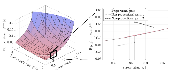
They are represented by means of the triple equivalent plastic strain, stress triaxiality and Lode angle parameter. According to Figure 9, these paths are non-proportional in this representation and even more important, they lead to different equivalent plastic strains at the final time corresponding to , see the zoom-in in Figure 9 (right). The deviation of the equivalent plastic strain for these paths is above . This deviation clearly confirms that a characterization and description of damage accumulation only by means of the three final influencing variables — equivalent plastic strain, stress triaxiality and Lode angle parameter — is generally not sufficient. This holds in particular if complex, non-proportional load paths are to be analyzed.
Since the path-dependent deviation of the fracture energy also relies on the underlying constitutive model, the numerical experiment is re-computed for the other models (ECC-a, ECC-i, LEM-a,LEM-i). Again it can be seen that the triple of equivalent plastic strain, stress triaxiality and Lode angle parameter does not uniquely define a damage state, see the results summarized in Figure 10.
4.2.3 Non-proportional load paths with constant stress invariants
According to the previous section, a damage characteriziation by means of the triple equivalent plastic strain, stress triaxiality and Lode angle parameter is usually not possible for complex load paths. Since the stress triaxiality and the Lode (angle) parameter are invariants of the stress tensor (see A), one could also monitor and control all three invariants of the stress tensor (instead of just and ). This is precisely the idea analyzed in this paragraph. For that purpose, two different stress tensors are considered. While corresponds to proportional loading, is associated with a more complex load path. However, both tensors show the same evolution of their invariants (eigenvalues ) – in particular and are identical for both paths. Only their directions are different (eigenvectors). and can be implemented by means of the spectral decomposition, i.e.,
| (51) | ||||
| (52) | ||||
| (53) |
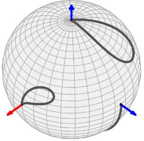
where are the eigenvectors of and are rotation matrices depending on the Euler angles , and . Four different mechanical tests are considered:
-
1.
Uniaxial tension: and
-
2.
Combined tension and shear: and
-
3.
Simple shear: and
-
4.
Combined compression and shear: and
While the first eigenvalue is increased, the second as well as the third follow from the prescribed and constant parameters and . To be more precise and as summarized in A are used. For the proportional load paths, stress tensor (51) with constant eigenvectors is considered and is increased up to a damage threshold of . In the case of the non-proportional load paths, the evolution of the Euler angles is summarized in Figure 11.
 \psfrag{e1}[c][c]{$\boldsymbol{e}_{x}$}\psfrag{e2}[c][c]{$\boldsymbol{e}_{y}$}\psfrag{e3}[c][c]{$\boldsymbol{e}_{z}$}\includegraphics[width=108.405pt]{Chapter/0X_NumericalResults/TensionShear/Figures/CoordinateSystemPSFRAG.eps}
In line with the example studied in the previous paragraph, the temporal discretization of is chosen such that all Euler angles vanish at final time as in Figure 11 when damage threshold is reached, i.e., the time scaling of and the Euler angles is synchronized.
The results of the numerical analyses are presented in Figure 12.
The bar charts summarize the results for all four models (ECC-a, ECC-i, LEM-a, LEM-i) and for all four mechanical tests (uniaxial tension, simple shear, combined tension and shear, combined compression and shear). It shows the relative difference of the equivalent plastic strain at final state between the proportional and the non-proportional load paths. It can be seen that the anisotropic model ECC-a leads to the largest difference – followed by its isotropic counterpart ECC-i. The sensitivity on the load path is less pronounced for the models LEM. However, a minor influence is still evident – even for model LEM-i. Focusing again on the fracture surface concept, Figure 12 shows that a characterization of material damage is still not possible by considering all three invariants of the stress tensor, together with the equivalent plastic strain. Otherwise, the relative distances in Figure 12 would vanish.
The presented numerical studies showed that a characterization of ductile damage by means of only the invariants of the stress tensor is usually not sufficient. This conclusion particularly applies to a characterization of damage by means of only the stress triaxiality or the Lode (angle) parameter. While for some load paths, such isotropic approximations might lead to reasonable predictions, they are usually inadequate for complex load paths.
5 Conclusion
Application limits of isotropic damage characterizations for complex load paths were investigated in this paper. For that purpose, a well-established anisotropic ductile damage model (Lemaitre model) depending on the complete stress tensor was considered first and its predicted response was analyzed for different load paths. Since such numerical experiments may depend on the underlying constitutive model, a second constitutive model was additionally employed.
The first numerical experiment – inspired by a coupled tension-torsion experiment – revealed that the frequently employed recommendation ”the smaller the stress triaxiality, the smaller the damage accumulation” can be wrong for complex load paths. In order to design paths contradicting this hypothesis, an algorithm was proposed to analyze differences in the predictions and unconsidered influences.
Starting from the invariant stress triaxiality, the Lode angle parameter was additionally controlled in the next example. Since the characterization of damage by means of the stress triaxiality and the Lode angle parameter is closely related to the concept of fracture surfaces, this concept was studied in detail. In particular, fracture surfaces were computed for both ductile damage models. Again, load paths were designed showing that a damage characterization by means of the extended set of influencing variables stress triaxiality, Lode angle parameter and equivalent plastic strain is often still not possible.
Finally, the full set of invariants of the stress tensor were controlled. This can be interpreted as an isotropic approximation. However, even in this more flexible case, load paths can be designed leading to different damage accumulation.
The numerical studies showed that damage can indeed be influenced and improved by controlling the stress triaxiality as well as the Lode angle parameter. However, the remaining coordinates of the load paths still have great potential for further improvement of damage accumulation and thus, control. This potential is to be further studied, e.g., in the context of forming processes. Furthermore, the numerical studies are to be further confirmed by real experiments.
Appendix A Parameter realization
Denoting the eigenvalues of the stress tensor as with and , the stress triaxiality and the Lode parameter are defined as
| (54) | ||||
| (55) |
These equations can be rewritten as
| (56) | ||||
| (57) |
with
and
They allow to enforce both the stress triaxiality as well as the Lode angle and to apply loading by increasing . Clearly, specical care is required, if .
Acknowledgements
Financial support from the German Research Foundation (DFG) via SFB/TR TRR 188 (project number 278868966), project C01, is gratefully acknowledged. We also gratefully acknowledge the computing time provided on the Linux HPC cluster at TU Dortmund University (LiDO3), partially funded in the course of the Large-Scale Equiment Initiative by the German Research Foundation (DFG) (project number 271512359).
References
- [1] R. I. Stephens, H. O. Fuchs (Eds.), Metal fatigue in engineering, 2nd Edition, A Wiley-Interscience publication, Wiley, New York Weinheim, 2001.
- [2] S. Ma, H. Yuan, Computational investigation of multi-axial damage modeling for porous sintered metals with experimental verification, Engineering Fracture Mechanics 149 (2015) 89–110. doi:10.1016/j.engfracmech.2015.09.049.
- [3] A. Tekkaya, P.-O. Bouchard, S. Bruschi, C. Tasan, Damage in metal forming, CIRP Annals 69 (2) (2020) 600–623. doi:10.1016/j.cirp.2020.05.005.
- [4] J. Koplik, A. Needleman, Void growth and coalescence in porous plastic solids, International Journal of Solids and Structures 24 (8) (1988) 835–853. doi:10.1016/0020-7683(88)90051-0.
- [5] A. Sancho, M. Cox, T. Cartwright, G. Aldrich-Smith, P. Hooper, C. Davies, J. Dear, Experimental techniques for ductile damage characterisation, Procedia Structural Integrity 2 (2016) 966–973. doi:10.1016/j.prostr.2016.06.124.
- [6] J. Lemaitre, A Continuous Damage Mechanics Model for Ductile Fracture, Journal of Engineering Materials and Technology 107 (1) (1985) 83–89. doi:10.1115/1.3225775.
- [7] A. L. Gurson, Continuum theory of ductile rupture by void nucleation and growth: Part i—yield criteria and flow rules for porous ductile media, Journal of Engineering Materials and Technology-transactions of The Asme 99 (1977) 2–15. doi:10.1115/1.3443401.
- [8] J. Simo, J.-W. Ju, Strain- and stress-based continuum damage models. i. formulation, International Journal of Solids and Structures 23 (1987) 821–840. doi:10.1016/0020-7683(87)90083-7.
- [9] M. Brünig, An anisotropic ductile damage model based on irreversible thermodynamics, International Journal of Plasticity 19 (10) (2003) 1679–1713. doi:10.1016/S0749-6419(02)00114-6.
- [10] P. Steinmann, I. Carol, A framework for geometrically nonlinear continuum damage mechanics, International Journal of Engineering Science 36 (15) (1998) 1793–1814. doi:10.1016/S0020-7225(97)00116-X.
- [11] M. Ekh, A. Menzel, K. Runesson, P. Steinmann, Anisotropic damage with the mcr effect coupled to plasticity, International Journal of Engineering Science 41 (13) (2003) 1535–1551, damage and failure analysis of materials. doi:10.1016/S0020-7225(03)00032-6.
- [12] T. Wierzbicki, Y. Bao, Y. Bai, A New Experimental Technique for Constructing a Fracture Envelope of Metals under Multi-axial loading, Proceedings of the 2005 SEM Annual Conference and Exposition on Experimental and Applied Mechanics (2005).
- [13] Y. Bai, T. Wierzbicki, A new model of metal plasticity and fracture with pressure and lode dependence, International Journal of Plasticity 24 (6) (2008) 1071–1096. doi:10.1016/j.ijplas.2007.09.004.
- [14] F. A. McClintock, A Criterion for Ductile Fracture by the Growth of Holes, Journal of Applied Mechanics 35 (2) (1968) 363–371. doi:10.1115/1.3601204.
- [15] J. Rice, D. Tracey, On the ductile enlargement of voids in triaxial stress fields, Journal of the Mechanics and Physics of Solids 17 (3) (1969) 201–217. doi:10.1016/0022-5096(69)90033-7.
- [16] A. Mattiello, R. Desmorat, Lode angle dependency due to anisotropic damage, International Journal of Damage Mechanics 30 (2) (2021) 214–259. doi:10.1177/1056789520948563.
- [17] R. Gitschel, O. Hering, A. Schulze, A. Erman Tekkaya, Controlling Damage Evolution in Geometrically Identical Cold Forged Parts by Counterpressure, Journal of Manufacturing Science and Engineering 145 (1) (2023) 011011. doi:10.1115/1.4056266.
- [18] A. Menzel, M. Ekh, P. Steinmann, K. Runesson, Anisotropic damage coupled to plasticity: Modelling based on the effective configuration concept, International Journal for Numerical Methods in Engineering 54 (10) (2002) 1409–1430. doi:10.1002/nme.470.
- [19] J. Lemaitre, R. Desmorat, Engineering Damage Mechanics. Ductile, Creep, Fatigue and Brittle Failure, 2005. doi:10.1007/b138882.
- [20] A. E. Green, P. M. Naghdi, A general theory of an elastic-plastic continuum, Archive for Rational Mechanics and Analysis 18 (4) (1965) 251–281. doi:10.1007/BF00251666.
- [21] B. Halphen, Q. S. Nguyen, Sur les matériaux standard généralisés, 1975.
- [22] C. Frederick, P. Armstrong, A Mathematical Representation of the Multiaxial Bauscinger Effect, Materials at High Temperatures 24 (2007) 1–26. doi:10.3184/096034007X207589.
- [23] K. Langenfeld, A. Schowtjak, R. Schulte, O. Hering, K. Möhring, T. Clausmeyer, R. Ostwald, F. Walther, A. Tekkaya, J. Mosler, Influence of anisotropic damage evolution on cold forging, Production Engineering 14 (01 2020). doi:10.1007/s11740-019-00942-y.
- [24] K. Langenfeld, K. Möhring, F. Walther, J. Mosler, On the regularization for ductile damage models, PAMM 19 (1) (2019) e201900003. doi:10.1002/pamm.201900003.
- [25] K. Langenfeld, J. Mosler, A micromorphic approach for gradient-enhanced anisotropic ductile damage, Computer Methods in Applied Mechanics and Engineering 360 (2020) 112717. doi:10.1016/j.cma.2019.112717.
- [26] A. E. Tekkaya, N. Ben Khalifa, O. Hering, R. Meya, S. Myslicki, F. Walther, Forming-induced damage and its effects on product properties, CIRP Annals 66 (1) (2017) 281–284. doi:10.1016/j.cirp.2017.04.113.
- [27] F. X. C. Andrade, M. Feucht, A. Haufe, F. Neukamm, An incremental stress state dependent damage model for ductile failure prediction, International Journal of Fracture 200 (1-2) (2016) 127–150. doi:10.1007/s10704-016-0081-2.
- [28] J. Kennedy, R. Eberhart, Particle swarm optimization, in: Proceedings of ICNN’95 - International Conference on Neural Networks, Vol. 4, 1995, pp. 1942–1948 vol.4. doi:10.1109/ICNN.1995.488968.
- [29] J. A. Nelder, R. Mead, A simplex method for function minimization, Comput. J. 7 (1965) 308–313. doi:10.1093/comjnl/7.4.308.